OGLE-2017-BLG-0537: Microlensing Event with a Resolvable Lens in $\lesssim 5$ years from High-resolution Follow-up Observations

Abstract

We present the analysis of the binary-lens microlensing event OGLE-2017-BLG-0537. The light curve of the event exhibits two strong caustic-crossing spikes among which the second caustic crossing was resolved by high-cadence surveys. It is found that the lens components with a mass ratio $\sim 0.5$ are separated in projection by $\sim 1.3\theta_{\rm E}$, where $\theta_{\rm E}$ is the angular Einstein radius. Analysis of the caustic-crossing part yields $\theta_{\rm E}=1.77\pm 0.16$ mas and a lens-source relative proper motion of $\mu=12.4\pm 1.1~{}{\rm mas}~{}{\rm yr}^{-1}$. The measured $\mu$ is the third highest value among the events with measured proper motions and $\sim 3$ times higher than the value of typical Galactic bulge events, making the event a strong candidate for follow-up observations to directly image the lens by separating it from the source. From the angular Einstein radius combined with the microlens parallax, it is estimated that the lens is composed of two main-sequence stars with masses $M_{1}\sim 0.4~{}M_{\odot}$ and $M_{2}\sim 0.2~{}M_{\odot}$ located at a distance of $D_{\rm L}\sim 1.2$ kpc. However, the physical lens parameters are not very secure due to the weak microlens-parallax signal, and thus we cross check the parameters by conducting a Bayesian analysis based on the measured Einstein radius and event timescale combined with the blending constraint. From this, we find that the physical parameters estimated from the Bayesian analysis are consistent with those based on the measured microlens parallax. Resolving the lens from the source can be done in about 5 years from high-resolution follow-up observations and this will provide a rare opportunity to test and refine the microlensing model.

1. Introduction

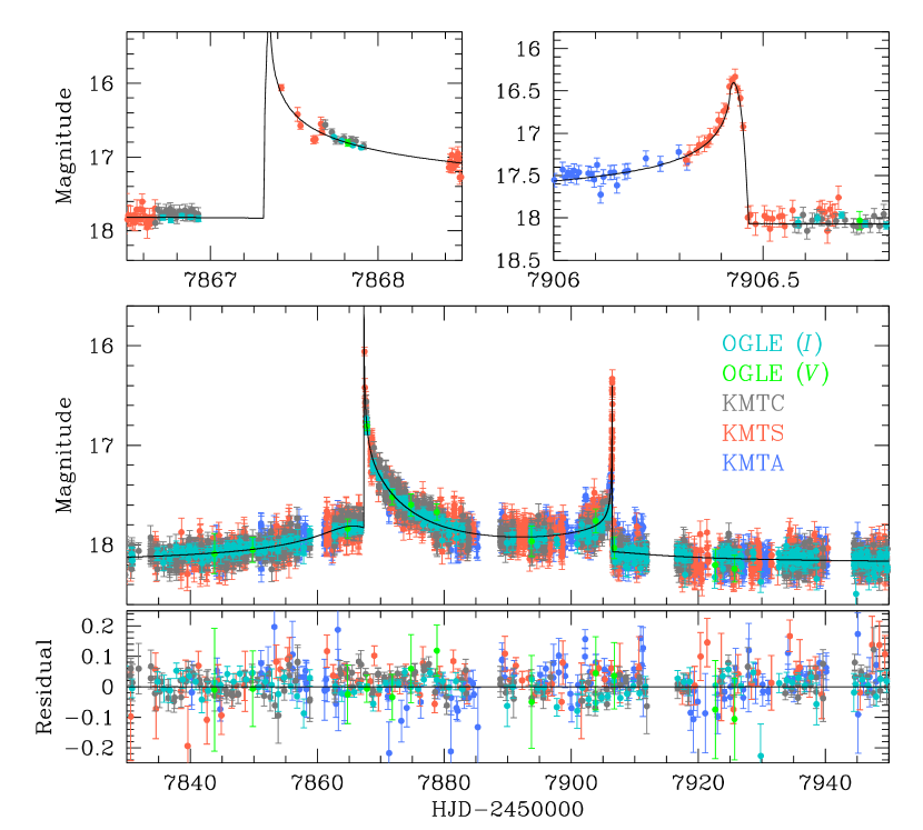
Figure 1.— Light curve of OGLE-2017-BLG-0537. The upper two panels show the zoom of the caustic-crossing parts of the light curve. The curve plotted over the data points is the model light curve. The bottom panel shows the residual from the model. To better show the residual, the data points are binned in one-day bins.

Currently, about 3000 microlensing events are annually being detected toward the Galactic bulge field by survey experiments (OGLE, MOA, KMTNet). The line of sight toward the bulge field passes through the region where the density of stars is very high and thus most lensing events are thought to be produced by stellar objects (Han & Gould, 2003).

Although stars are the major population of lensing objects, it is difficult to directly observe them. The most important reason for this difficulty is the slow motion of the lens with respect to the lensed star (source). For typical galactic lensing events produced by low-mass stars, the relative lens-source proper motion is $\mu\sim 5~{}{\rm mas}~{}{\rm yr}^{-1}$. This implies that one has to wait $\sim 10$ – 20 years to resolve the lens from the source even from observations using currently available instrument with the highest resolution, e.g., the Hubble Space Telescope (HST) with $\sim 0.1^{\prime\prime}$ resolution and ground-based Keck adaptive optics (AO) with $\sim 0.05^{\prime\prime}$ resolution. In addition, the most common population of lenses are low-mass bulge M dwarfs, which have apparent magnitudes fainter than $I\sim 22$. Considering that lensing events are detected toward dense fields where stellar images are severely blended, it is difficult to observe these faint lens objects.

As an alternate method to reduce the waiting time for the lens-source resolution, Bennett et al. (2007) proposed a method using the combination of the ground-based data and the data from high-resolution follow-up observations. In the first step of this method, the source flux is estimated from the analysis of the lensing light curve obtained from ground-based observations, usually taken in optical bands. In the second step, the optical source flux is converted to the photometric system of high-resolution data, which is usually taken in near-infrared (NIR) passbands. Then, the lens flux is identified as an excess flux measured by subtracting the converted source flux from the flux of the target measured in the high-resolution data. This method has been applied to the planetary system OGLE-2007-BLG-368L to estimate the mass of the planet host (Sumi et al., 2010). However, the lens flux estimated by this so-called ‘single-epoch’ method is subject to large uncertainties due to the multi-step optical-to-NIR flux conversion procedure combined with the difficulty of aligning the ground-based and high-resolution images (Henderson et al., 2014). Furthermore, it is difficult to completely rule out companions to the source or lens as well as ambient stars as being the origin of excess light, e.g., MOA-2008-BLG-310 (Janczak et al., 2010).

Lens identification from direct imaging has been studied and actual observations have been conducted. Based on the physical and dynamical models of the Galaxy, Han & Chang (2003) estimated the fraction of high proper-motion events for which the lens and source can be resolved from high-resolution observations. From this, they found that lenses can be resolved for $\sim 3$ and 22 per cent of disk-bulge events and for $\sim 0.3$ and 6 per cent of bulge self-lensing events from follow-up observations using an instrument with $0.1^{\prime\prime}$ resolving power to be conducted 10 and 20 years after events, respectively. By inspecting events detected from 2004 to 2013, Henderson et al. (2014) presented a list of 20 lensing events with relative lens-source proper motions greater than $\sim 8~{}{\rm mas}~{}{\rm yr}^{-1}$ as candidates of follow-up observations for direct lens imaging. For 3 lensing events, the lenses were actually detected. These events include MACHO-LMC-5 (Alcock et al., 2001), MACHO-95-BLG-37 (Kozłowski et al., 2007), and OGLE-2005-BLG-169 (Batista et al., 2015; Bennett et al., 2015). Among them, MACHO-LMC-5 was detected toward the Large Magellanic Cloud field and the others were detected toward the bulge field. The lenses of the two MACHO events were resolved from HST observations, while the lens of OGLE-2005-BLG-169 was detected from Keck AO observations.

In this paper, we present the analysis of the microlensing event OGLE-2017-BLG-0537. The event was produced by a binary lens and the light curve of the event exhibits characteristic caustic-crossing features. Despite its very short duration, one of the caustic crossings was resolved by high-cadence lensing surveys and we measure the relative lens-source proper motion from the analysis of the light curve. It is found that the proper motion is $\sim 3$ times bigger than the value of typical galactic bulge events. The high proper motion combined with the close distance to the lens makes the event a strong candidate for follow-up observations to directly identify the lens.

2. Observations

The source star of the lensing event OGLE-2017-BLG-0537 is located toward the Galactic bulge field with the equatorial coordinates $({\rm RA},{\rm DEC})_{\rm J2000}=$(17:56:47.75,-28:15:37.8), which correspond to the galactic coordinates $(l,b)=(1.83^{\circ},-1.76^{\circ})$. The baseline magnitude of the event before lensing magnification was $I_{\rm base}=18.15$.

The brightening of the source flux induced by gravitational lensing was first noticed from observations conducted by the Optical Gravitational Lensing Experiment (OGLE: Udalski et al., 2015a) survey. The OGLE observations were carried out in $I$ and $V$ passbands using the 1.3m telescope located at the Las Campanas Observatory in Chile.

The event was also in the field of the Microlensing Telescope Network (KMTNet: Kim et al., 2016) survey. The KMTNet observations were conducted using three identical 1.6m telescopes that are globally distributed in the Cerro Tololo Interamerican Observatory in Chile, the South African Astronomical Observatory in South Africa, and the Siding Spring Observatory in Australia. We refer the three KMTNet telescopes as KMTC, KMTS, and KMTA, respectively. KMTNet data were taken also in $I$ and $V$ bands. The $V$-band data are used mainly to measure the color of the source star. The event is cataloged (Kim et al., 2018a, b) by KMTNet as BLG02M0506.017562 and lies in two slightly offset fields BLG02 and BLG42 with a combined cadence of $\Gamma=4\,{\rm hr}^{-1}$.

Data obtained by the OGLE and KMTNet surveys are processed using the photometry codes of the individual groups. Both codes are based on the Difference Image Analysis (DIA) developed by Alard & Lupton (1998) and customized by the individual groups: Udalski (2003) and Albrow et al. (2009) for the OGLE and KMTNet photometry codes, respectively. Since the data sets of the individual groups are processed using different photometry codes, we renormalize the error bars of the data following the recipe described in Yee et al. (2012).

In Figure 1, we present the light curve of the event. The light curve exhibits two strong spikes that are characteristic features of caustic-crossing binary-lens events. The caustic crossings occurred at ${\rm HJD}^{\prime}={\rm HJD}-2450000\sim 7867.4$ and 7906.4. The facts that the time gap between the caustic-crossing spikes, $\sim 39$ days, is very long compared to the duration of the event and that the caustic crossings occurred when the lensing magnification was low suggest that the projected separation between the lens components is similar to the angular Einstein radius. Such a ‘resonant’ binary lens forms a single big closed caustic curve, and the two spikes were produced when the source entered and exited the caustic curve. The first caustic crossing could have been observed by the KMTA telescope but no observation was conducted due to bad weather. However, the second caustic crossing was captured by the KMTS data thanks to the high-cadence coverage of the field. Resolving the caustic crossing enables one to measure the normalized source radius $\rho=\theta_{*}/\theta_{\rm E}$, where $\theta_{*}$ and $\theta_{\rm E}$ represent the angular radii of the source star and the Einstein ring, respectively. With external information about $\theta_{*}$, one can then measure $\theta_{\rm E}$.

Although the overall light curve has a typical shape of a caustic-crossing binary-lens event, we note that the event is very unusual in the sense that the duration of caustic-crossing is very short. The caustic-crossing timescale measured during the caustic exit is $t_{\rm cc}\sim 0.5$ hr. The caustic-crossing timescale is related to the relative lens-source proper motion by

$$\mu\simeq{\theta_{*}\over t_{\rm cc}}{1\over\sin\psi},$$ (1)

where $\psi$ represents the angle between the source trajectory and the fold of the caustic curve. For stars located in the bulge, the angular radius is $\theta_{*}\sim 5~{}\mu{\rm as}$ for giants and $\sim 0.5~{}\mu{\rm as}$ for main-sequence stars. Then, the measured caustic-crossing timescale indicates $\mu\sim 10~{}{\rm mas}~{}{\rm yr}^{-1}$ even for a faint main-sequence source star and assuming a right-angle caustic entrance of the source trajectory, i.e., $\psi=90^{\circ}$. This relative lens-source proper motion is significantly greater than those of typical lensing events.

3. Light Curve Modeling

Considering that the two spikes are the characteristic features of binary-lens events, we model the observed light curve with a binary-lens interpretation. Under the assumption that the relative lens-source motion does not experience any acceleration, i.e., rectilinear motion, binary lensing light curves are described by 7 parameters. Four of these parameters describe the lens-source approach, including the time of the closest source-lens approach, $t_{0}$, the impact parameter of the approach, $u_{0}$, the event timescale, $t_{\rm E}$, and the angle between the source trajectory and the binary axis, $\alpha$. We use the center of mass of the binary lens as the reference position on the lens plane, and the impact parameter is normalized to the angular Einstein radius. Another two parameters describe the binary lens including the projected separation, $s$ (normalized to $\theta_{\rm E}$), and the mass ratio, $q$, between the binary lens components. Since the event exhibits features of caustic crossings, during which the light curve is affected by finite-source effects, one needs an additional parameter of the normalized source radius $\rho$ to account for these effects.

Due to the large number of lensing parameters, it is difficult to find the best-fit solution from a full-scale grid search. We, therefore, utilize a hybrid approach. In this approach, we divide the lensing parameters into two groups of grid $(s,q)$ and downhill parameters $(t_{0},u_{0},t_{\rm E},\alpha,\rho)$. This division is based on the fact that lensing magnifications are sensitive to the small changes of the grid parameters, while magnifications vary smoothly with the change of the downhill parameters. With this division of parameters, we conduct a grid search in the space of the grid parameters and, for a given set of the grid parameters, we search for the other parameters around the circle in the seed values of $\alpha$ using a downhill approach based on the Markov Chain Monte Carlo (MCMC) method. The grid search yields a $\chi^{2}$ map in the space of the grid parameters. From the map, we identify local minima. In the next step, we refine the individual local solutions by allowing all parameters to vary. We then find the global solution by comparing $\chi^{2}$ values of the individual local minima.

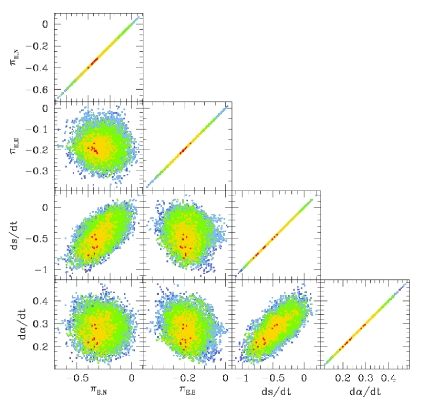
Figure 2.— $\Delta\chi^{2}$ distributions of MCMC chains for the combinations of the higher-order lensing parameters $\pi_{{\rm E},N}$, $\pi_{{\rm E},E}$, $ds/dt$, and $d\alpha/dt$. Dots with different color represent chains with $\Delta\chi^{2}<1$ (red), $<4$ (yellow), $<9$ (green), $<16$ (cyan), and $<25$ (blue).

From the initial search, we find 2 local solutions with event timescales of $t_{\rm E}\sim 54$ days and 90 days, respectively. Among the two local solutions, we exclude the latter solution because (1) it yields a poorer fit than the former solution by $\Delta\chi^{2}\sim 50$ and (2) it requires abnormally large higher-order effects to describe the observed light curve while the former solution well describes the observed light curve without introducing the higher-order effects. According to the best-fit solution, the event was produced by a binary with a projected separation $s\sim 1.2$ and a mass ratio $q\sim 0.4$.

The event lasted $\sim 100$ days, which comprises an important portion of Earth’s orbital period. In this case, the assumption of the rectilinear lens-source motion may not be valid. Two factors can cause non-rectilinear motion. One is the orbital motion of Earth, ‘microlens-parallax’ effect (Gould, 1992), and the other is the orbital motion of the binary lens, ‘lens-orbital’ effect (Albrow et al., 2000). We check the possibility of these higher-order effects by conducting additional modeling. Accounting for the microlens-parallax effect in lensing modeling requires including two additional lensing parameters of $\pi_{{\rm E},N}$ and $\pi_{{\rm E},E}$, which denote the two components of the microlens-parallax vector $\mbox{\boldmath$\pi$}_{\rm E}$ along the north and east equatorial coordinates, respectively. In parallax modeling, there can exist a pair of degenerate solutions with $u_{0}>0$ and $u_{0}<0$ due to the mirror symmetry of the source trajectory with respect to the binary axis: “ecliptic degeneracy” (Smith et al., 2003; Skowron et al., 2011). We, therefore, consider both $u_{0}>0$ and $u_{0}<0$ when parallax effects are considered in modeling. Considering the lens-orbital effect also requires including additional parameters. Under the approximation that the positional changes of the lens components during the event are small, the effect is described by two parameters of $ds/dt$ and $d\alpha/dt$, which represent the change rates of the binary separation and the source trajectory angle, respectively. We note that detecting microlens-parallax effects is important because the physical parameters of the lens mass, $M$, and distance to the lens, $D_{\rm L}$, are uniquely determined from the measured microlens parallax in combination with the angular Einstein radius by

$$M={\theta_{\rm E}\over\kappa\pi_{\rm E}};\qquad D_{\rm L}={{\rm au}\over\pi_{\rm E}\theta_{\rm E}+\pi_{\rm S}},$$ (2)

where $\kappa=4G/(c^{2}{\rm au})$, $\pi_{\rm S}={\rm au}/D_{\rm S}$, and $D_{\rm S}$, represents the distance to the source.

We find that the higher-order effects in the observed light curve are minor. It is found that the fit improves by $\Delta\chi^{2}\sim 3.7$ and $\sim 4.1$ with the consideration of the microlens-parallax and the lens-orbital effects, respectively. When both effects are simultaneously considered, the improvement is $\Delta\chi^{2}\sim 8.6$. In Figure 2, we present $\Delta\chi^{2}$ distributions of MCMC chains for the combinations of the higher-order lensing parameters, i.e., $\pi_{{\rm E},N}$, $\pi_{{\rm E},E}$, $ds/dt$, and $d\alpha/dt$. The distributions show no strong correlations among the parameters. The improvement of the fit, i.e., $\Delta\chi^{2}\sim 8.6$, mathematically corresponds to $\sim 3\sigma$, but such a level of fit improvement can be ascribed to noise in data. We, therefore, cross check the result by comparing the physical parameters resulting from the measured $\pi_{\rm E}$ with those estimated from Bayesian analysis. See detailed discussion in Section 4.

Table 1Best-fit lensing parameters

Parameter	$u_{0}>0$	$u_{0}<0$
$t_{0}$ (HJD′)	7880.795 $\pm$ 0.495	7880.684 $\pm$ 0.583
$u_{0}$	0.138 $\pm$ 0.007	-0.131 $\pm$ 0.008
$t_{\rm E}$ (days)	51.99 $\pm$ 0.61	52.21 $\pm$ 0.53
$s$	1.28 $\pm$ 0.01	1.27 $\pm$ 0.01
$q$	0.50 $\pm$ 0.02	0.49 $\pm$ 0.03
$\alpha$ (rad)	-0.595 $\pm$ 0.012	0.573 $\pm$ 0.005
$\rho$ ($10^{-3}$)	0.381 $\pm$ 0.020	0.389 $\pm$ 0.020
$\pi_{{\rm E},N}$	-0.34 $\pm$ 0.11	0.19 $\pm$ 0.10
$\pi_{{\rm E},E}$	-0.19 $\pm$ 0.05	-0.26 $\pm$ 0.03
$ds/dt$ (yr -1)	-0.74 $\pm$ 0.19	-0.33 $\pm$ 0.18
$d\alpha/dt$ (yr -1)	0.20 $\pm$ 0.05	-0.26 $\pm$ 0.06
$F_{s}$	0.096 $\pm$ 0.001	0.096 $\pm$ 0.001
$F_{b}$	0.753 $\pm$ 0.001	0.751 $\pm$ 0.001

Note. — ${\rm HJD}^{\prime}={\rm HJD}-2450000$.

In Table 1, we list the lensing parameters of the event. Although the higher-order parameters are not securely measured, we present the solutions resulting from the models considering the higher-order effects. It is found that the solution with $u_{0}>0$ is slightly favored over the solution with $u_{0}<0$ by $\Delta\chi^{2}\sim 3.0$. We note that the lensing parameters of the two solutions with $u_{0}>0$ and $u_{0}<0$ are roughly in the relation of $(u_{0},\alpha,\pi_{{\rm E},N},d\alpha/dt)\leftrightarrow-(u_{0},\alpha,\pi_{{\rm E},N},d\alpha/dt)$ due to the mirror symmetry of the source trajectories between the two solutions. The uncertainties of the individual parameters are estimated from the scatter of points in the MCMC chain. Also presented are the fluxes of the source, $F_{s}$, and blend, $F_{b}$. The flux values are normalized to the flux of a star with $I=18$, i.e., $F=10^{-0.4(I-18)}$, where $I$ represents the $I$-band magnitude. The $F_{s}$ and $F_{b}$ values show that the blend is $\sim 8$ times brighter than the source, indicating that the event is heavily blended.

To be noted among the determined lensing parameter is that the normalized source radius $\rho\sim 0.38\times 10^{-3}$ is unusually small. The value of the normalized source radius for typical lensing events is $\rho\sim(1-2)\times 10^{-2}$ for a giant source star and $\rho\sim(1-2)\times 10^{-3}$ for a main-sequence source star. We find that the source is a main-sequence star located in the bulge (see Section 4.1). Then, the measured value of $\rho$ is smaller than the value of typical lensing events by a factor $\gtrsim 3$.

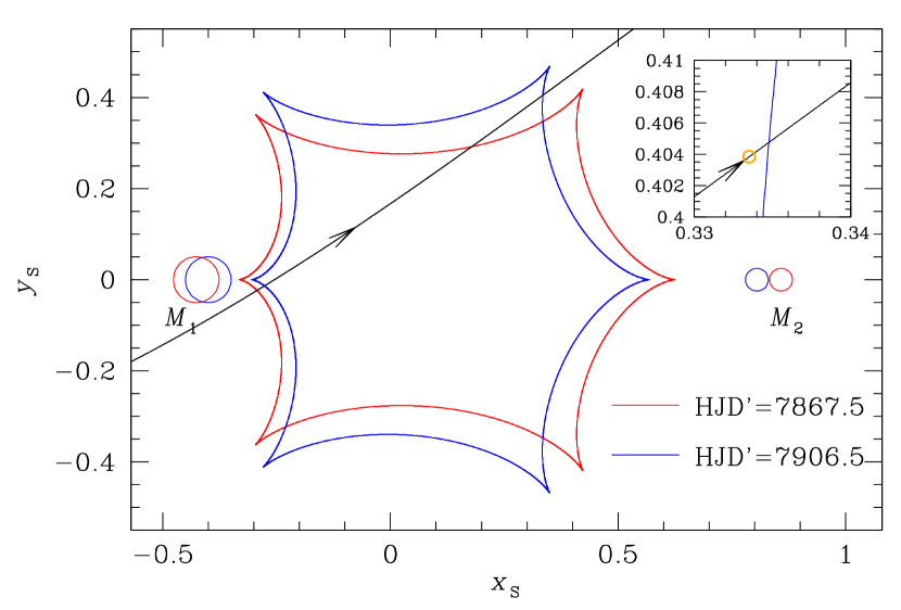
Figure 3.— Lens system configuration in which the source trajectory (line with an arrow) is shown with respect to the caustic (cuspy closed curve) and the binary lens components (marked by $M_{1}$ and $M_{2}$). We present the lens positions and caustics at two epochs of ${\rm HJD}^{\prime}=7867.5$ and 7906.5, which correspond to the times of the first and second caustic spikes, respectively. Lengths are scaled to the angular Einstein radius corresponding to the total mass of the binary lens, and the coordinates are centered at the center of mass of the lens. The inset shows the zoom of the caustic region at the time of the source star’s caustic exit. The small circle, whose size is scaled to the source size, indicates the source.

In Figure 3, we present the configuration of the lens system in which the source trajectory (line with an arrow) with respect to the caustic (cuspy closed curve) and the positions of the lens components (marked by $M_{1}$ and $M_{2}$) are presented. We note that the lens positions and the resulting caustic vary in time due to the lens-orbital effect. We, therefore, present the lens positions and caustics at two epochs of ${\rm HJD}^{\prime}=7867.5$ and 7906.5, which correspond to the times of the first and second caustic spikes, respectively. As predicted, the binary lens forms a resonant caustic due to the closeness of the binary separation to unity, $s\sim 1.28$. The caustic forms a closed curve with 6 folds. The two spikes in the observed light curve were produced by the source star’s crossings over the lower left and upper right folds of the caustic. The model light curve of the solution and the residual from the model are presented in Figure 1.

4. Constraining the Lens

4.1. Angular Einstein Radius

Measurement of the normalized source radius $\rho$ leads to determination of the angular Einstein radius by the relation

$$\theta_{\rm E}={\theta_{*}\over\rho}.$$ (3)

For the $\theta_{\rm E}$ determination, then, it is required to estimate the angular source radius $\theta_{*}$.

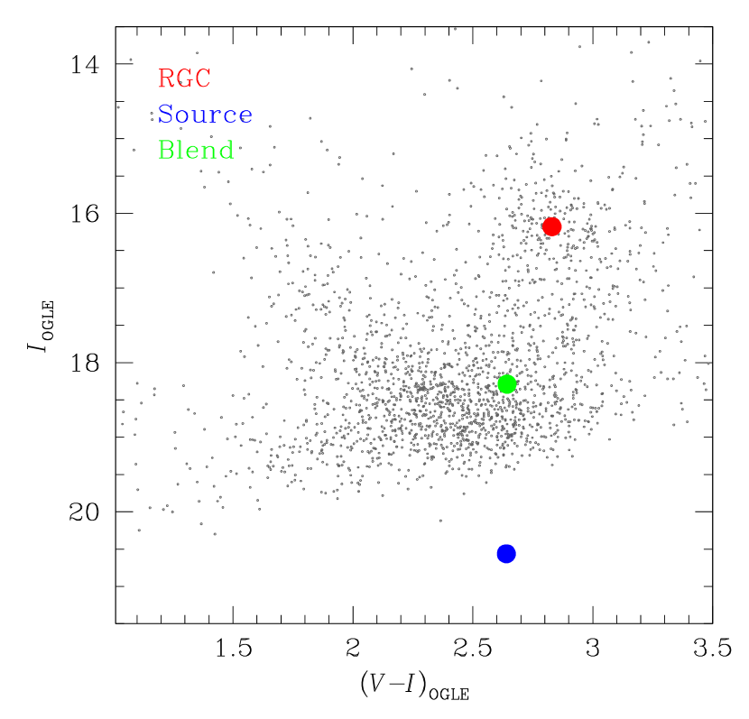
Figure 4.— Source location with respect to the centroid of red giant clump (RGC) in the instrumental color-magnitude diagram. Also marked is the position of the blend.

We estimate the angular radius of the source star based on the color and brightness. To measure the de-reddened color $(V-I)_{0}$ and brightness $I_{0}$ from the uncalibrated color-magnitude diagram (CMD), we use the method described in Yoo et al. (2004). In this method, the centroid of red giant clump (RGC), whose de-reddened color and brightness $(V-I,I)_{\rm RGC,0}=(1.06,14.35)$ (Bensby et al., 2011; Nataf et al., 2013) are known, is used as a reference for the calibration of the color and brightness. Figure 4 shows the source location in the instrumental CMD. The instrumental color and magnitude of the source are $(V-I,I)=(2.64\pm 0.03,20.56\pm 0.01)$. According to the minimum caustic magnification theorem, the minimum lensing magnification when the source is inside caustic is $A_{\rm min}=3$ (Witt & Mao, 1995). With this constraint combined with the measured brightness at the bottom of U-shape trough ($I\sim 17.9$ at ${\rm HJD}^{\prime}\sim 7855$), the upper limit of the source brightness is set to be $I_{\rm upper}\sim 19.1$ assuming that all the light comes from the source, i.e., no blending. The measured source brightness, $I\sim 20.6$, is fainter than $I_{\rm upper}$ and thus satisfies this constraint. We measure the source color by simultaneously fitting the OGLE $I$ and $V$-band data sets to the best-fit model. In Figure 1, we plot the OGLE $V$-band data (green dots) used for the source color determination. With the measured offsets in color $(V-I)=-0.19$ and brightness $\Delta I=4.38$ of the source with respect to those of the RGC centroid, we determine that the de-reddened color and brightness of the source star are $(V-I,I)_{{\rm S},0}=(0.87\pm 0.03,18.73\pm 0.01)$. This indicates that the source is an early K-type main-sequence star. We estimate the angular source radius by converting the $V-I$ color into $V-K$ color using the color-color relation of Bessell & Brett (1988) and then using the $(V-K)/\theta_{*}$ relation of Kervella et al. (2004). From this procedure, it is estimated that the source has an angular radius of $\theta_{*}=0.68\pm 0.05~{}\mu{\rm as}$. Combined with the measured value of $\rho$, we estimate that the angular Einstein radius corresponding to the total mass of the lens is

$$\theta_{\rm E}=1.77\pm 0.16~{}{\rm mas}.$$ (4)

Once the angular Einstein radius is determined, the relative lens-source proper motion is determined with the event timescale by

$$\mu_{\rm geo}={\theta_{\rm E}\over t_{\rm E}}=12.4\pm 1.1~{}{\rm mas}~{}{\rm yr}^{-1},$$ (5)

and

$$\mu_{\rm hel}=\left|\mbox{\boldmath$\mu$}_{\rm geo}+{\bf v}_{\oplus,\perp}{\pi_{\rm rel}\over{\rm au}}\right|=11.0\pm 1.0~{}{\rm mas}~{}{\rm yr}^{-1},$$ (6)

where $\mbox{\boldmath$\mu$}_{\rm geo}=\mu_{\rm geo}(\mbox{\boldmath$\pi$}_{\rm E}/\pi_{\rm E})$ and $\mbox{\boldmath$\mu$}_{\rm hel}$ represent the relative lens-source motion vectors measured in the geocentric and heliocentric frames, respectively, and ${\bf v}_{\oplus,\perp}=(-1.6,-21.5)~{}{\rm km}~{}{\rm s}^{-1}$ is the velocity of the Earth motion projected on the sky at $t_{0}$. The position angle of $\mbox{\boldmath$\mu$}_{\rm hel}$ is $\sim 196^{\circ}$ and $\sim 314^{\circ}$ as measured from the north for the $u_{0}>0$ and $u_{0}<0$ solutions, respectively. In Table 2, we summarize the values of $\theta_{\rm E}$, $\mu_{\rm geo}$, and $\mu_{\rm hel}$ for the $u_{0}>0$ and $u_{0}<0$ solutions. We note that the estimated geocentric proper motion is bigger than the heuristically estimated value $\mu\sim 10~{}{\rm mas}~{}{\rm yr}^{-1}$ in Section 2 because the caustic entrance angle of the source trajectory $\psi\sim 53^{\circ}$ is different from the assumption of the right-angle entrance. See the zoom of caustic region at the moment of the source star’s caustic exit presented in the inset of Figure 3.

We note that the estimated angular Einstein radius is significantly bigger than the values of typical lensing events. For the most common population of galactic bulge events (with $D_{\rm L}\sim 6$ kpc) produced by low-mass stars (with $M\sim 0.4~{}M_{\odot}$), the angular Einstein radius is $\theta_{\rm E}\sim 0.4$ mas. Then, the measured angular Einstein radius is $\sim 4.4$ times bigger than the typical value. The angular Einstein radius is related to the physical lens parameters by

$$\theta_{\rm E}=\sqrt{\kappa M\pi_{\rm rel}};\qquad\pi_{\rm rel}={\rm au}\left({1\over D_{\rm L}}-{1\over D_{\rm S}}\right).$$ (7)

Since $\theta_{\rm E}\propto M^{1/2}$ and $\theta_{\rm E}\propto\pi_{\rm rel}^{-1/2}$, the large value of $\theta_{\rm E}$ indicates that the lens is either very heavy or located close to the observer. The large angular Einstein radius leads to the high relative lens-source proper motion because $\mu\propto\theta_{\rm E}$. As we will discuss in the following subsection, the high proper motion makes the event an important target for high-resolution follow-up observations for direct detection of the lens.

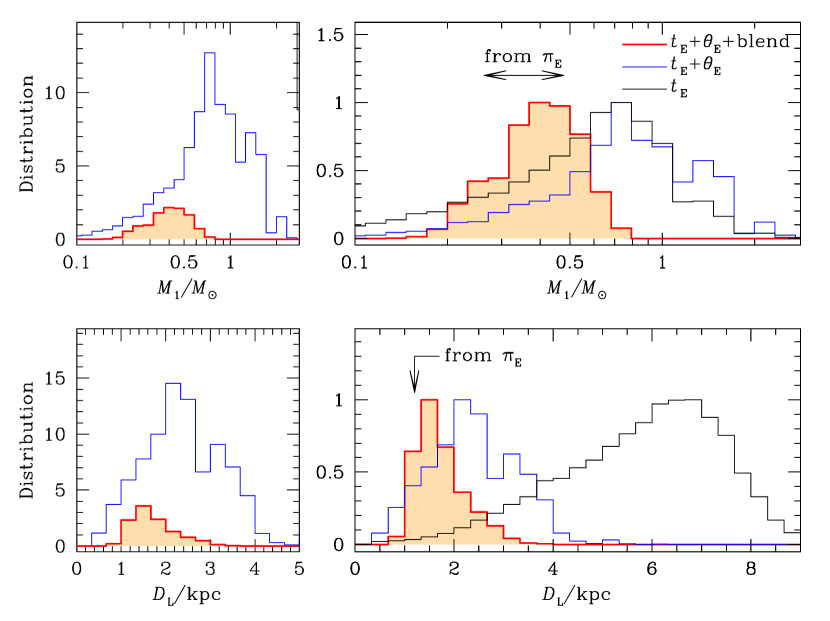
Figure 5.— The probability distributions of the primary mass (upper panels) and distance to the lens (lower panels) obtained by Bayesian analysis. The 3 curves in black, blue, and red colors represent the distributions obtained with only the event timescale constraint, with timescale plus angular Einstein radius constraint, and with the additional constraint of the blended light, respectively. The distributions in the left panels are relatively scaled, while the distributions in the right panels are scaled so that the peak of the distribution becomes unity. The lens mass and distance marked by “from $\pi_{\rm E}$” represent the values estimated from the measured microlens parallax.

4.2. Physical Lens Parameters: Based on $\pi_{\rm E}$

Although the measured microlens parallax $\pi_{\rm E}$ is subject to some uncertainty due to the weak parallax signal, we estimate the physical lens parameters based on the parallax parameters combined with the measured angular Einstein radius using the relations in Equation (2). In Table 2, we present the estimated parameters. Here $M_{1}$ and $M_{2}$ ($<M_{1}$) represent the masses of the individual lens components. The projected separation between the lens components is computed by $a_{\perp}=sD_{\rm L}\theta_{\rm E}$. According to the estimated masses of the lens components, the lens consists of an early and a mid M-type dwarfs with masses $M_{1}\sim 0.4~{}M_{\odot}$ and $M_{2}\sim 0.2~{}M_{\odot}$, respectively. As anticipated by the large angular Einstein radius, it is estimated that the lens is located at a close distance of $D_{\rm L}\sim 1.2$ – 1.5 kpc.

Also presented in Table 2 is the projected kinetic-to-potential energy ratio, (KE/PE)_⟂. The ratio is computed based on the measured lensing parameters of $s$, $ds/dt$, and $d\alpha/dt$ by

$$\left({{\rm KE}\over{\rm PE}}\right)_{\perp}={(a_{\perp}/{\rm au})^{3}\over 8\pi(M/M_{\odot})}\left[\left({1\over s}{ds/dt\over{\rm yr}^{-1}}\right)^{2}+\left({d\alpha/dt\over{\rm yr}^{-1}}\right)^{2}\right].$$ (8)

In order for the lens to be a bound system, the ratio should be less than unity. It is found that both $u_{0}>0$ and $u_{0}<0$ solutions meet this requirement.

Table 2Physical Lens Parameters (from $\pi_{\rm E}$)

Parameter	$u_{0}>0$	$u_{0}<0$	Bayesian
$\theta_{\rm E}$ (mas)	$1.77\pm 0.16$	$1.73\pm 0.16$	-
$\mu_{\rm geo}$ (mas yr-1)	$12.4\pm 1.1$	$12.1\pm 1.1$	-
$\mu_{\rm hel}$ (mas yr-1)	$11.0\pm 1.0$	$10.3\pm 0.9$	-
$M_{1}$ ($M_{\odot}$)	$0.37\pm 0.10$	$0.44\pm 0.11$	$0.43\pm 0.14$
$M_{2}$ ($M_{\odot}$)	$0.18\pm 0.05$	$0.22\pm 0.06$	$0.22\pm 0.07$
$D_{\rm L}$ (kpc)	$1.2\pm 0.3$	$1.5\pm 0.3$	$1.8^{+0.6}_{-0.4}$
$a_{\perp}$ (au)	$2.8\pm 0.6$	$3.2\pm 0.7$	$3.5^{+1.2}_{-0.8}$
(KE/PE)⟂	0.18	0.09	-

4.3. Physical Lens Parameters: Bayesian Approach

The lens parameters determined in the previous subsection are not very secure due to the uncertain microlens parallax value. We, therefore, cross check the physical parameters by additionally conducting a Bayesian analysis of the event based on the measured event timescale and the angular Einstein radius combined with the blended light. We note that the blended light provides a constraint because the lens cannot be brighter than the blend.

For the Bayesian analysis, one needs models of the mass function and the physical and dynamical distributions of lens and source. In the analysis, we use the Chabrier (2003) mass function. In the mass function, we include stellar remnants. Following the model of Gould (2000), we assume that stars with masses $1~{}M_{\odot}\leq M\leq 8~{}M_{\odot}$, $8~{}M_{\odot}\leq M\leq 40~{}M_{\odot}$, $M\geq 40~{}M_{\odot}$, have evolved into white dwarfs (with a mean mass $\langle M\rangle\sim 0.6~{}M_{\odot}$), neutron stars ($\langle M\rangle\sim 1.36~{}M_{\odot}$), black holes ($\langle M\rangle\sim 5~{}M_{\odot}$), respectively. For the physical distributions of lens objects, we use the density model of Han & Gould (2003), in which the Galaxy is described by a double-exponential disk and a triaxial bulge. To describe the motion of the lens and source, we use the dynamical model of Han & Gould (1995), in which disk objects move following a gaussian distribution with a mean corresponding to the disk rotation speed and bulge objects move according to a triaxial Gaussian distribution with velocity components determined by tensor virial theorem based on the bulge shape.

With the adopted model distributions, we produce a large number of mock lensing events by conducting Monte Carlo simulation in which the mass of the primary lens is drawn from the model mass function. We then construct the distributions of the lens mass and distance for events with lens masses and distances fall in the ranges of the measured event time scale and angular Einstein radius, and with lens brightness fainter than the blend. We note that the constraints of the time scale and angular Einstein radius are based on the values corresponding to the primary of the lens, i.e., $t_{{\rm E},1}=t_{\rm E}/\sqrt{1+q}$ and $\theta_{{\rm E},1}=\theta_{\rm E}/\sqrt{1+q}$, under the assumption that binary components follow the same mass function as that of single stars. Then, the mass and distance are estimated as the median values and their uncertainties are estimated based on the 16/84 percentiles of the distributions.

Figure 5 shows the probability distributions of the primary mass (upper panels) and distance to the lens (lower panels). To show the how the individual constraints, i.e., $t_{\rm E}$, $\theta_{\rm E}$, and blended light, contribute to characterize the physical lens parameters, we present 3 distributions: with only the event timescale constraint (marked by “$t_{\rm E}$”), with the timescale plus angular Einstein radius constraint (“$t_{\rm E}+\theta_{\rm E}$”), and with the additional constraint of the blended light (“$t_{\rm E}+\theta_{\rm E}+$ blend”). We note that the distributions in the left panels are relatively scaled, while the distributions in the right panels are scaled so that the peak of the distribution becomes unity. From the comparison of the distributions, it is found that the angular Einstein radius gives a strong constraint on the distance to the lens. This is because $\theta_{\rm E}\propto\pi_{\rm rel}^{1/2}\propto(D_{\rm L}^{-1}-D_{\rm S}^{-1})^{1/2}$ and thus nearby lenses can result in large angular Einstein radius. On the other hand, the blended light provides an important constraint on the lens mass. Although heavy lenses (with $M_{1}\gtrsim 0.8\ M_{\odot}$) can produce events with large $\theta_{\rm E}$, they are excluded by the constraint of the lens brightness. The blend constraint also excludes very nearby lenses (with $D_{\rm L}\lesssim 1$ kpc).

The masses of the primary and the companion estimated by the Bayesian analysis are

$$M_{1}=0.43\pm 0.14\ M_{\odot}$$ (9)

and

$$M_{2}=0.22\pm 0.07\ M_{\odot}.$$ (10)

We note that the lens masses span wide ranges, $0.29\lesssim M_{1}/M_{\odot}\lesssim 0.57$ and $0.15\lesssim M_{2}/M_{\odot}\lesssim 0.29$ (as measured in $1\sigma$ level), due to the nature of the Bayesian mass estimation. The lens components are separated in projection by

$$a_{\perp}=3.5_{-0.8}^{+1.2}\ {\rm au}.$$ (11)

The estimated distance to the lens is

$$D_{\rm L}=1.8_{-0.4}^{+0.6}\ {\rm kpc},$$ (12)

indicating that the lens is located at a close distance. We list the physical lens parameters estimated from the Bayesian analysis in Table 2.

We note that the physical lens parameters estimated based on the measured microlens parallax match well those estimated from the Bayesian analysis. In Figure 5, we mark the lens mass and distance estimated from $\pi_{\rm E}$ on the probability distributions obtained from the Bayesian analysis. It is found that both the lens mass and distance are positioned close to the highest probability regions of the Bayesian distributions. This indicates that the microlens parallax is correctly measured despite the weak signal in the lensing light curve.

5. Direct Lens Imaging

The scientific importance of the event lies in the fact that the event provides a rare opportunity to test the microlensing model from follow-up observations. The main reason for the event to be a good target for checking the lensing parameters is that the lens can be resolved from the source and thus directly imaged within a reasonably short period of time after the event. The measured proper motion, $\mu=12.4\pm 1.0~{}{\rm mas}~{}{\rm yr}^{-1}$, of the event is the third highest value among the events with measured proper motions after OGLE-2007-BLG-224, with $\mu=48\pm 2~{}{\rm mas}~{}{\rm yr}^{-1}$ (Gould et al., 2009), and LMC-5, with $\mu=21.4\pm 0.7~{}{\rm mas}~{}{\rm yr}^{-1}$ (Alcock et al., 2001; Drake et al., 2004; Gould et al., 2004). We also note that the event has the second-largest well-measured angular Einstein radius of published lensing events after OGLE-2011-BLG-0417 (Shin et al., 2012). See Henderson et al. (2014) and Penny et al. (2016) for the compilation of events with well measured angular Einstein radii. Batista et al. (2015) pointed out that a lens can be resolved from a source on Keck images when the separation between the lens and source is $\sim 50$ – 60 mas. Applying the same criterion, then, the lens of OGLE-2017-BLG-0537 can be resolved from Keck AO imaging if follow-up observations are conducted $\gtrsim 4$ years after the event.

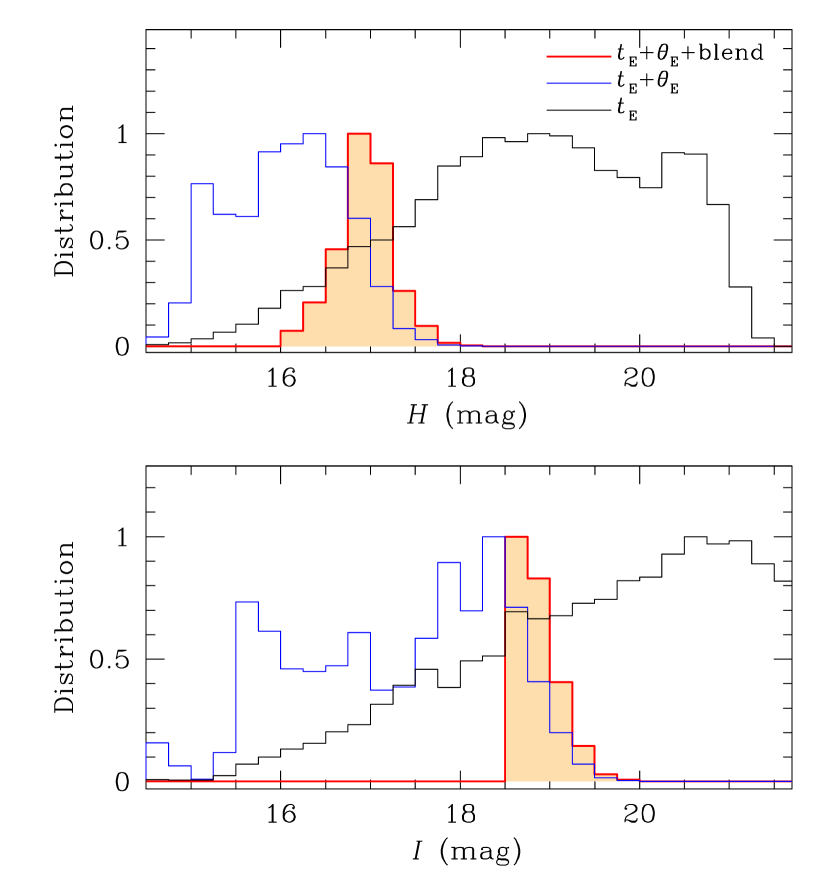
Figure 6.— The probability distributions of the $H$ and $I$-band brightness of the lens. Notations are same as those in Figure 5.

Another reason that makes the event favorable for high-resolution follow-up observations is the closeness of the lens. The most common population of lenses are low-mass stars. Then, if an event is produced by such a lens located at a large distance, e.g., bulge lens, it would be difficult to image the lens. In the case of OGLE-2017-BLG-0537, the lens will be bright enough for direct imaging because of its small distance despite that the lens components are M dwarfs. In Figure 6, we present the distribution of the lens brightness estimated from the Bayesian analysis. We estimate $H$-band brightness because follow-up observations will be conducted in NIR bands. In the Bayesian simulation, we estimate $H$-band magnitude using the relation

$$H=M_{V}-(V-H)+5\log D_{\rm L}/{\rm pc}-5+A_{H}.$$ (13)

Here we estimate the absolute $V$-band magnitude, $M_{V}$, from the mass using the mass-luminosity relation and use $V-H$ color from from Bessell & Brett (1988). We assume $A_{H}\sim 0.108A_{V}$ (Nishiyama et al., 2008), where $A_{V}\sim 3.3$ is obtained from the OGLE extinction map. The estimated range of the $H$-band brightness of the lens is

$$H=17.1_{-0.33}^{+0.28}.$$ (14)

In comparison, the $H$-band source brightness is $H_{\rm S}\sim 18.0$.

We note that the apparent brightness of the blend, $I_{b}\sim 18.3$, matches well the lens brightness estimated by Bayesian analysis, $I_{\rm L}\sim 18.5$. This indicates that the blend light is likely to come from the lens. Under this assumption, prompt high-resolution imaging can potentially constrain the lens properties without needing to wait. See Henderson (2015) for detailed discussion.

There exist several cases in which lensing models are checked by follow-up observations. The first example is OGLE-2005-BLG-169 in which a weak and short-term anomaly in the lensing light curve was produced by a lens with a Neptune mass ratio planetary companion (Gould et al., 2006). From the Keck AO observation conducted $\sim 8$ years after the discovery of the event, the lens and source were completely resolved, proving a precise measurement of the relative lens-source motion (Batista et al., 2015). This confirmed and refined the lensing model and ruled out a range of solutions that were allowed by the microlensing light curve. The lensing solution of the event was additionally confirmed from follow-up observations conducted using HST (Bennett et al., 2015). Another case where lensing solution was checked by follow-up observations is the binary event OGLE-2011-BLG-0417. Microlensing analysis of the event yielded not only the lens mass and distance but also a complete Keplerian solutions including the radial velocity of the binary lens orbital motion (Shin et al., 2012). This led to the proposal of follow-up spectroscopic observations for Doppler radial velocity measurement to test the lensing solution (Gould et al., 2013). Boisse et al. (2015) actually conducted the proposed radial-velocity measurement of the event using UVES spectroscopy mounted on the VLT, but this measurement did not confirm the microlensing prediction for the binary lens system. Using the spectral energy distribution combined with the high-resolution images obtained from successive follow-up spectroscopic and AO observations of the event, Santerne (2016) concluded that the lens parameters were not compatible with the ones obtained from lensing analysis, raising the need to check the lensing solution. Additionally, the lensing parameters of the planetary event OGLE-2014-BLG-0124 determined by Udalski et al. (2015b) were confirmed and refined by follow-up AO imaging observation conducted by Beaulieu et al. (2018).

6. Conclusion

We analyzed the microlensing event OGLE-2017-BLG-0537, in which the light curve exhibited two strong caustic-crossing spikes. It was found that the event was produced by a binary lens for which the lens components with a mass ratio $q\sim 0.5$ was separated in projection by $s\sim 1.3$. Among the two caustic-crossing spikes, the second caustic crossing was resolved by high-cadence surveys. Analysis of the caustic-crossing part of the light curve yielded an angular Einstein radius of $\theta_{\rm E}=1.77\pm 0.16$ mas and a lens-source relative proper motion of $\mu=12.4\pm 1.1~{}{\rm mas}~{}{\rm yr}^{-1}$. The measured proper motion was the third highest value among the events with measured proper motions and $\sim 3$ times higher than the value of typical galactic bulge events. This makes the event a strong candidate for follow-up observations to directly image the lens from the source.

From the angular Einstein radius combined with the microlens parallax, it was estimated that the lens was composed of two main-sequence stars with masses $M_{1}\sim 0.4~{}M_{\odot}$ and $M_{2}\sim 0.2~{}M_{\odot}$ located at a distance of $D_{\rm L}\sim 1.2$ kpc, but the physical lens parameters were not very secure due to the weak microlens-parallax signal. We cross checked the physical parameters by additionally conducting a Bayesian analysis based on the measured Einstein radius and event timescale combined with the blending constraint. From this, we found that the physical parameters estimated from the Bayesian analysis were consistent with those based on the measured microlens parallax. Resolving the lens from the source can be done in about 5 years from high-resolution follow-up observations and this will provide a rare opportunity to test the microlensing model and refine lens parameters.

References

- Alard & Lupton (1998) Alard, C., & Lupton, R. H. 1998, ApJ, 503, 325
- Albrow et al. (2000) Albrow, M. D., Beaulieu, J.-P., Caldwell, J. A. R., et al. 2000, ApJ, 534, 894
- Albrow et al. (2009) Albrow, M. D., Horne, K., Bramich, D. M., et al. 2009, MNRAS, 397, 2099
- Alcock et al. (2001) Alcock, C., Allsman, R. A., Alves, D. R., et al. 2001, Nature, 414, 617
- Batista et al. (2015) Batista, V., Beaulieu, J.-P., Bennett, D. P., et al. 2015, ApJ, 808, 170
- Beaulieu et al. (2018) Beaulieu, J.-P., Batista, V., Bennett, D. P. 2018, AJ, 155, 78
- Bennett et al. (2007) Bennett, D. P., Anderson, J., & Gaudi, B. S. 2007, ApJ, 660, 781
- Bennett et al. (2015) Bennett, D. P., Bhattacharya, A., Anderson, J., et al. 2015, ApJ, 808, 169
- Bensby et al. (2011) Bensby, T., Adén, D., Meléndez, J., et al. 2011, PASP, 533, 134
- Bessell & Brett (1988) Bessell, M. S., & Brett, J. M. 1988, PASP, 100, 1134
- Boisse et al. (2015) Boisse, I., Santerne, A., Beaulieu, J.-P., Fakhardji, W., Santos, N. C., Figueira, P., Sousa, S. G., Ranc, C. 2015, A&A, 582, L11
- Chabrier (2003) Chabrier, G. 2003, ApJ, 586, L133
- Drake et al. (2004) Drake, A. J., Cook, K. H., & Keller, S. C. 2004, ApJ, 607, L29
- Gould (1992) Gould, A. 1992, ApJ, 392, 442
- Gould (2000) Gould, A. 2000, ApJ, 535, 928
- Gould et al. (2004) Gould, A., Bennett, D. P., & Alves, D. R. 2004, ApJ, 614, 404
- Gould et al. (2013) Gould, A., Shin, I.-G., Han, C., Udalski, A., & Yee, J. C. 2013, ApJ, 768, 126
- Gould et al. (2006) Gould, A., Udalski, A., An, D. 2006, ApJ, 644, L37
- Gould et al. (2009) Gould, A., Udalski, A., Monard, B., et al. 2009, ApJ, 698, L147
- Han & Chang (2003) Han, C., & Chang, H.-Y. 2003, MNRAS, 338, 637
- Han & Gould (2003) Han, C., & Gould, A. 2003, ApJ, 592, 172
- Han & Gould (1995) Han, C., & Gould, A. 1995, ApJ, 447, 53
- Henderson (2015) Henderson, C. B. 2015, ApJ, 800, 58
- Henderson et al. (2014) Henderson, C. B., Park, H., Sumi, T., et al. 2014, ApJ, 794, 71
- Janczak et al. (2010) Janczak, J., Fukui, A., Dong, S., et al. 2010, ApJ, 711, 731
- Kervella et al. (2004) Kervella, P., Thévenin, F., Di Folco, E., & Ségransan, D. 2004, A&A, 426, 297
- Kozłowski et al. (2007) Kozłowski, S., Woźniak, P. R., Mao, S., & Wood, A. 2007, ApJ, 671, 420
- Kim et al. (2018a) Kim, D.-J., Kim, H.-W., Hwang, K.-H., et al. 2018a, AJ, 155, 76
- Kim et al. (2018b) Kim, H.-W., Hwang, K.-H., Kim, D.-J., et al. 2018b, in preparation
- Kim et al. (2016) Kim, S.-L., Lee, C.-U., Park, B.-G., et al. 2016, JKAS, 49, 37
- Nataf et al. (2013) Nataf, D. M., Gould, A., Fouqué, P., et al. 2013, ApJ, 769, 88
- Nishiyama et al. (2008) Nishiyama, S., Nagata, T., Tamura, M., Kandori, R., Hatano, H., Sato, S., & Sugitani, K. 2008, ApJ, 680, 1174
- Penny et al. (2016) Penny, M. T., Henderson, C. B., & Clanton, C. 2016, ApJ, 830, 150
- Santerne (2016) Santerne, A., Beaulieu, J.-P., Rojas Ayala, B., et al. 2016, A&A, 595, L11
- Shin et al. (2012) Shin, I.-G., Han, C., Choi, J.-Y., et al. 2012, ApJ, 755, 91
- Skowron et al. (2011) Skowron, J., Udalski, A., Gould, A., et al. 2011, ApJ, 738, 87
- Smith et al. (2003) Smith, M. C., Mao, S., & Paczyński, B. 2003, MNRAS, 339, 925
- Sumi et al. (2010) Sumi, T., Bennett, D. P., Bond, I. A., et al. 2010, ApJ, 710, 1641
- Udalski (2003) Udalski, A. 2003, Acta Astron., 53, 291
- Udalski et al. (2015a) Udalski, A., Szymański, M. K., & Szymaḿski, G. 2015, Acta Astron., 65, 1
- Udalski et al. (2015b) Udalski, A., Yee, J. C., Gould, A., et al. 2015, ApJ, 799, 237
- Witt & Mao (1995) Witt, H. J., & Mao, S. 1995, ApJ, 447, L105
- Yee et al. (2012) Yee, J. C., Shvartzvald, Y., Gal-Yam, A., et al. 2012, ApJ, 755, 102
- Yoo et al. (2004) Yoo, J., DePoy, D. L., Gal-Yam, A., et al. 2004, ApJ, 603, 139