Bulk scaling in wall-bounded and homogeneous vertical natural convection

Abstract

Previous numerical studies on homogeneous Rayleigh–Bénard convection, which is Rayleigh–Bénard convection (RBC) without walls, and therefore without boundary layers, have revealed a scaling regime that is consistent with theoretical predictions of bulk-dominated thermal convection. In this so-called asymptotic regime, previous studies have predicted that the Nusselt number (Nu) and the Reynolds number ($\Rey$) vary with the Rayleigh number (Ra) according to $\mbox{{Nu}}\sim\mbox{{Ra}}^{1/2}$ and $\Rey\sim\mbox{{Ra}}^{1/2}$ at small Prandtl number ($\Pran$). In this study, we consider a flow that is similar to RBC but with the direction of temperature gradient perpendicular to gravity instead of parallel; we refer to this configuration as vertical natural convection (VC). Since the direction of the temperature gradient is different in VC, there is no exact relation for the average kinetic dissipation rate, which makes it necessary to explore alternative definitions for Nu, $\Rey$ and Ra and to find physical arguments for closure, rather than making use of the exact relation between Nu and the dissipation rates as in RBC. Once we remove the walls from VC to obtain the homogeneous setup, we find that the aforementioned $1/2$-power-law scaling is present, similar to the case of homogeneous RBC. When focussing on the bulk, we find that the Nusselt and Reynolds numbers in the bulk of VC too exhibit the $1/2$-power-law scaling. These results suggest that the $1/2$-power-law scaling may even be found at lower Rayleigh numbers if the appropriate quantities in the turbulent bulk flow are employed for the definitions of Ra, $\Rey$ and Nu. From a stability perspective, at low- to moderate-Ra, we find that the time-evolution of the Nusselt number for homogenous vertical natural convection is unsteady, which is consistent with the nature of the elevator modes reported in previous studies on homogeneous RBC.

1 Introduction

Thermally driven flows play a crucial role in nature and are associated with many engineering flows. To study such flows, researchers typically consider idealised setups which include (figure 1a) the classical Rayleigh–Bénard convection, or RBC (Ahlers+others.2009; Lohse+Xia.2010; Chilla+Schumacher.2012), where fluid is confined between a heated bottom plate and a cooled upper plate, (figure 1b) horizontal convection, or HC (Hughes+Griffiths.2008; Shishkina+Grossmann+Lohse.2016), where fluid is heated at one part of the bottom plate and cooled at some other part, and (figure 1c) vertical natural convection, or VC (Ng+Ooi+Lohse+Chung.2014; Ng+Ooi+Lohse+Chung.2017), where fluid is confined between two vertical walls, one heated and one cooled, i.e. the flow is driven by a horizontal average heat flux. Alternative configurations of the VC flow, such as in a confined cavity (Patterson+Armfield.1990; Yu+Li+Ecke.2007) and in a confined cylinder (Shishkina+Horn.2016; Shishkina.2016.momentum) have also been investigated. In all these studies on thermal convection, there is a common interest to physically understand and predict how the temperature difference imposed on the flow (characterised by the Rayleigh number Ra) influences the heat flux (characterised by the Nusselt number Nu) and the degree of turbulence (characterised by the Reynolds number $\Rey$). With such relations, one is able to avoid relying on empirical relationships that are undetermined outside the range of calibration and which ignore the underlying physics.

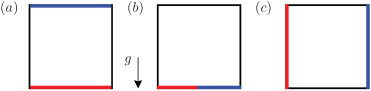
Figure 1: Examples of wall-bounded configurations for ($a$) Rayleigh–Bénard convection (RBC) ($b$) horizontal convection (HC) and ($c$) vertical natural convection (VC). For illustration purposes, the configurations are drawn in a cavity with aspect ratio equal to one. Heated walls are indicated in red and cooled walls in blue. $g$ is the gravity vector.

At high Ra, Kraichnan.1962 and Grossmann+Lohse.2000; Grossmann+Lohse.2001; Grossmann+Lohse.2002; Grossmann+Lohse.2004 – hereinafter referred to as the GL theory – predicted the so-called asymptotic ultimate-regime scaling where Nu∼Ra^1/2,  ∼Ra^1/2, for low $\Pran$-values, for instance, when $\Pran\leqslant 1$. (The $\Pran$-dependence of $\mbox{{Nu}}\sim\Pran^{1/2}$ and $\Rey\sim\Pran^{-1/2}$ predicted by the GL theory for this asymptotic ultimate regime was confirmed in Calzavarini+others.2005 in the case of homogeneous RBC. For homogeneous VC, the $\Pran$-dependence is expected to be the same, but is beyond the scope of this paper.) These scaling relations contain logarithmic corrections when boundary layers or plumes are prominent (Grossmann+Lohse.2011). In numerical studies that seek to model only bulk thermal convection, i.e. without boundary layers, the $1/2$-power-law scalings were indeed subsequently reported: Lohse+Toschi.2003 and Calzavarini+others.2005; Calzavarini+others.2006 discounted the influence of boundary layers by simulating a triply periodic configuration for RBC, termed homogeneous RBC. Schmidt+others.2012 numerically studied the same flow but with lateral (no-slip) confinement and also reported the $1/2$-power-law scaling despite the presence of lateral boundary layers. In experiments, bulk convection is mimicked by measuring plate-free convection, i.e. in a vertical channel connecting a hot chamber at the bottom and a cold chamber at the top (Gibert+others.2006; Gibert+others.2009; Tisserand+Others.2010), or by measuring fluid mixing in a long vertical pipe (Cholemari+Arakeri.2009). The use of alternative length scales to recover the $1/2$-power scaling in the bulk-dominated flow has also been suggested (Gibert+others.2006; Gibert+others.2009). Later, Riedinger+Tisserand+others.2013 conducted experiments by tilting the vertical channel and in doing so introduced a gravitational component which is orthogonal to the axis of the channel. The study reported a $1/2$-power slope at high Ra and low channel tilt angle (relative to the vertical). Recently, Frick+others.2015 investigated the effect of tilting in a sodium-filled cylinder of aspect ratio equal to $5$ with a heated lower plate and a cooled upper plate. The study found that the heat transfer is more effective when the cylinder is tilted by $45^{\circ}$ compared to when the cylinder is tilted by $0^{\circ}$ and $90^{\circ}$. Shishkina+Horn.2016 obtained similar results in their numerical study where they compared RBC and VC by gradually tilting a fully enclosed cylindrical vessel. Using the same cylindrical vessel, Shishkina.2016.momentum then found that the effective power-law scaling in VC is smaller than $1/2$ because of geometrical confinement.

In the present study, we investigate the scaling relations of VC in a triply periodic domain (figure 2$c$ and $d$) using an approach that is similar to previous studies on bulk scaling for RBC ( Lohse+Toschi.2003; Calzavarini+others.2005). The numerical setup of this homogeneous flow is described in § LABEL:sec:ComputParam. Our objective is to determine whether the asymptotic ultimate $1/2$-power-law scaling can similarly be found in an idealised setup of VC which is free of influences from the boundary layers. To achieve this, we adopted two approaches: (i) homogeneous VC with a constant mean temperature and velocity gradient in the horizontal direction, which we denote as HVC (figure 2$c$), and (ii) homogeneous VC with only a constant horizontal mean temperature gradient and no velocity gradient (or shear), which we denote as HVCws (figure 2$d$). Although the flow in (i) closely resembles the characteristics of the bulk flow in VC, we emphasize that the homogeneous and wall-bounded setups are different because for the homogeneous case, the energy transport to the walls is absent. In addition, the flow in ($ii$) without shear is evidently fictitious since a velocity gradient is present in the bulk of VC. In other words, both homogeneous cases (i) and (ii) are simplifications of VC, simplifications that are amenable to the $1/2$-power-law scaling arguments as has been shown previously for homogeneous RBC ( Lohse+Toschi.2003).

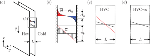
Figure 2: ($a$) Setup of VC. ($b$) Illustration of the mean temperature profile (top) and mean streamwise velocity profile (bottom). Both mean profiles are statistically antisymmetric about the channel centreline. ($c$) Setup of HVC with a mean temperature and velocity gradient. ($d$) Setup of HVCws with only a mean temperature gradient. The black slopes in ($c$) and ($d$) represent the temperature gradient $\Delta_{b}/L$, whereas the red slope in ($c$) represents the uniform mean shear $u_{b}/L$. Note that in ($a$), periodicity is applied in $x$- and $y$-directions only, whereas in ($c$) and ($d$), periodicity is applied in all three directions, illustrated by the dashed boundaries.

The paper is structured as follows: We begin by describing the respective dynamical equations for HVC and HVCws in § 2, which are numerically solved. Using scaling arguments, we relate both HVC and HVCws with the asymptotic ultimate $1/2$-power-law scaling in § 3. In § LABEL:sec:ComputParam, we outline the numerical setups and direct numerical simulation (DNS) datasets, the latter of which is used to test the assumptions employed in our scaling arguments. Then, to assist comparisons with VC, we compare the dynamical lengthscales of HVC and HVCws with VC in § LABEL:sec:CompareStatistics. In § LABEL:sec:ScalingRelations, we compute the scaling of turbulent quantities of the homogeneous setups and show that Nu and $\Rey$ appear to follow the $1/2$-power-law scaling, just as in homogeneous RBC and consistent with the theoretical predictions by Kraichnan.1962, the GL-theory and the scaling arguments in § 3. Inspired by the scaling of the turbulent quantities, we apply the insight gained to VC and find that the scaling of the turbulent bulk quantities in VC also exhibit the $1/2$-power-law scaling. Finally, in § LABEL:sec:ExponentialGrowth, we compare the stability of the solutions for HVCws and homogeneous RBC, the latter of which is known to exhibit unstable, so-called ‘elevator modes’ at low Rayleigh numbers. Such modes are associated with exponentially growing values of Nu followed by sudden break-downs (Calzavarini+others.2005; Calzavarini+others.2006) and have been reported in similar studies, such as in laterally confined and axially homogeneous RBC (Schmidt+others.2012). In § LABEL:sec:CompareToDNS, when we compared the stability analyses to data from our DNS of HVCws, we find that the unsteady solutions are also present in HVCws at low Ra, but nonetheless both Nu and $\Rey$ appear to follow the $1/2$-power-law scaling.

2 Dynamical equations

We begin with the general form of the governing equations for VC, where we invoke the Boussinesq approximation so that the density fluctuations are considered small relative to the mean. The governing continuity, momentum and energy equations for the velocity field $u_{i}(x_{i},t)$ and the temperature field $\varTheta(x_{i},t)$ are respectively given by, ∂uj∂xj &= 0,
∂ui∂t + ∂ujui∂xj = -1ρ0∂p∂xi + ν∂2ui∂xj2 + gβ(Θ-Θ_0)δ_i1,
∂Θ∂t + ∂uiΘ∂xi = κ∂2Θ∂xi2. The coordinate system $x$, $y$ and $z$ (or $x_{1}$, $x_{2}$ and $x_{3}$) refers to the vertical streamwise direction that is opposite to gravity, spanwise and wall-normal directions, respectively. The pressure field is denoted by $p(x_{i},t)$. For VC (see figure 2$a$), we define $\varTheta_{0}=(T_{h}+T_{c})/2$ as the reference temperature, $\Delta\equiv T_{h}-T_{c}$ the temperature difference between the two walls, which are separated by a distance $L$, and $g$ as the gravitational acceleration. For the fluid, we specify $\beta$ as the coefficient of thermal expansion, $\nu$ as the kinematic viscosity and $\kappa$ as the thermal diffusivity, all assumed to be independent of temperature. The Rayleigh and Prandtl numbers are then respectively defined as Ra≡gβΔL^3/(νκ), ≡ν/κ, and the Nusselt and Reynolds numbers are respectively defined as Nu≡JL/(Δκ), ≡UL/ν, where $J\equiv-\kappa(\mathrm{d}\overline{\varTheta}/\mathrm{d}z)+\overline{w^{\prime}\varTheta^{\prime}}$ the horizontal heat flux and $U$ is a characteristic velocity scale. Equations (2$a$–$c$) have been numerically solved in Ng+Ooi+Lohse+Chung.2014 for no-slip and impermeable boundary conditions for the velocity field at the walls (in the plane $z=0$ and $z=L$) and periodic boundary conditions in the $x$- and $y$-directions. The resulting mean streamwise velocity component ($\overline{u}=u-u^{\prime}$) and mean temperature ($\overline{\varTheta}=\varTheta-\varTheta^{\prime}$) are statistically antisymmetric about the channel centreline, as illustrated in figure 2($b$). Here, we denote time- and $xy$-plane-averaged quantities with an overbar, and the corresponding fluctuating part with a prime. In the channel-centre of VC, both $\mathrm{d}\overline{u}/\mathrm{d}z$ and $\mathrm{d}\overline{\varTheta}/\mathrm{d}z$ are finite and possesses the same sign. Note that in VC, $\overline{u}$ is a persistent non-zero mean quantity, which is different to RBC: for a sufficiently long time-average, it can be shown that the wall-parallel-averaged velocity components in RBC are statistically zero ( vanReeuwijk+Jonker+Hanjalic.2008).

For the present study, we are interested in two numerical setups that are different from VC. The new setups are defined such that they allow us to directly test the $1/2$-power scaling relations described in (1). From this line of reasoning, the associated governing equations of the new setups should be expected to obey the scaling arguments of Kraichnan.1962 and Grossmann+Lohse.2000, and in the spirit of deriving (1). In short, the key idea here is to design numerical setups that only solve the fluctuating components of VC, which conveniently emulates the turbulent bulk-dominated conditions expected in the asymptotic ultimate regime of thermal convection at very high Ra (Grossmann+Lohse.2000). To this end, we describe two setups for VC, i.e.   HVC and HVCws, which are inspired by the so-called homogeneous configurations for RBC of Lohse+Toschi.2003 and Calzavarini+others.2005; Calzavarini+others.2006. Different to homogeneous RBC, the HVC and HVCws setups described in the following sections are subjected to a mean horizontal temperature (or buoyancy) gradient, which is orthogonal to gravity.

2.1 Homogeneous vertical natural convection with shear (HVC)

For HVC, we assume that the flow is decomposed into constant mean gradients and fluctuations. These assumptions are notionally similar to the flow conditions in the channel-centre of VC, as illustrated in figures 2($b$) and 2($c$). To describe the numerical approach, we also make use of the equation of state for gases, $\beta(\varTheta-\varTheta_{0})\approx-(1/\rho_{0})(\rho-\rho_{0})$ and introduce $b$ the buoyancy variable. Therefore, following Chung+Matheou.2012, we write -(g/ρ_0) (ρ-ρ_0) &= N^2 x_3 + b^′,
u_i = S δ_i1 x_3 + u_i^′,
p + ρ_0 g x_1 = p^′ where $N^{2}\equiv\mathrm{d}\overline{b}/\mathrm{d}z=g\beta\mathrm{d}\overline{\varTheta}/\mathrm{d}z$ the constant mean buoyancy gradient, $S\equiv\mathrm{d}\overline{u}/\mathrm{d}z$ the (temporally) uniform mean shear and $u_{i}^{\prime}$, $b^{\prime}$ and $p^{\prime}$ are the fluctuations of velocity, buoyancy and pressure, respectively. Substituting (2.1) into (2), we obtain ∂uj′∂xj &= 0,
∂b′∂t + N^2 u_3^′+ ∂uj′b′∂xj + Sδ_j1x_3 ∂b′∂xj = κ∂2b′∂xj2
∂ui′∂t + Sδ_i1u_3^′+ ∂uj′ui′∂xj + S δ_j1x_3 ∂ui′∂xj = -1ρ0∂p′∂xi + ν∂2ui′∂xj2 + (N^2x_3 + b^′) δ_i1. The methodology to solve (2.1$a$–$c$) closely follows the approach by Chung+Matheou.2012, that is, a skewing coordinate $\xi_{i}(x_{i},t)=x_{i}-St\delta_{i1}x_{3}$ is introduced to transform the dependent variables $\{b^{\prime},u_{i}^{\prime},p^{\prime}\}(x_{i},t)=\{\widetilde{b},\widetilde{u}_{i},\widetilde{p}\}(\xi_{i}(x_{i},t),t)$ to convert (2.1) to ∂~uj∂~ξj &= 0,
∂~b∂t + N^2~u_3 + ∂~uj~b∂~ξj = κ∂2~b∂~ξj2,
∂~ui∂t + Sδ_i1~u_3 + ∂~uj~ui∂~ξj = -1ρ0∂~p∂~ξi + ν∂2~ui∂~ξj2 + (N^2 ξ_3 + ~b) δ_i1, where $\partial/\partial\widetilde{\xi}_{i}\equiv\partial/\partial\xi_{i}-St\delta_{i3}\partial/\partial\xi_{1}$.

The transformation from (2.1) to (2.1) allows us to numerically solve (2.1) in a triply periodic domain provided $N^{2}\xi_{3}$ the non-periodic term on the right-hand-side of (2.1$c$), which acts on the streamwise momentum, can be neglected. This is satisfied if $|N^{2}\xi_{3}|\ll|\widetilde{b}|$. Estimating $|\widetilde{b}|=O(b_{rms})$, the inequality then holds true for scales in the $z$-direction that are smaller than $b_{rms}/N^{2}(=\varTheta_{rms}(\mathrm{d}\overline{\varTheta}/\mathrm{d}z)^{-1})$. There is no straightforward method to determine beforehand if $b_{rms}/N^{2}$ is larger or smaller than $L_{z}$ without performing the homogeneous simulations. As a start, we omit the non-periodic term from our DNS, noting that this is a necessary numerical approximation. On the other hand, if $b_{rms}/N^{2}<L_{z}$, the solutions based on the DNS without the non-periodic term are still meaningful, provided we focus only on the dynamics of the scales that are $\lesssim b_{rms}/N^{2}$. Indeed, we will show in § LABEL:subsec:Assumptions that $b_{rms}/N^{2}<L_{z}$ for the homogeneous cases, which we then further enforce in our calculations of the Nusselt and Reynolds number in § LABEL:subsec:ScalingOfNuAndRe, where we apply a spectral filter to the Nusselt and Reynolds number using a cut-off length of the order of $b_{rms}/N^{2}$, smaller than $L_{z}$.

The solutions to (2.1) without the non-periodic term describe the evolution of the fluctuating quantities of VC under the influence of a prescribed mean buoyancy gradient and mean shear. We acknowledge that the aforementioned assumptions are merely simplifications since both the mean shear $S$ and the buoyancy gradient $N^{2}$ are in principle the responding parameters of the bulk flow of VC; the boundary layers that form at the walls determine $S$ and $N^{2}$. Thus, an explicit relation between $S$ and $N^{2}$ is presently unknown, at least to our knowledge. Similarly, in the case of HVC, both $S$ and $N^{2}$ are not known a priori but must be prescribed. (This is detailed in § LABEL:sec:ComputParam). We emphasize that the formulation for HVC above is not an attempt to simulate the bulk flow of VC — it is instead an idealised numerical model that is designed to test the $1/2$-power-law scalings of (1).

2.2 Homogeneous vertical natural convection without shear (HVCws)

In addition to HVC, HVCws is an alternative numerical setup that can test the $1/2$-power-law scalings by assuming that the mean shear component $S$ in (2.1$b$) is zero, i.e.  $u_{i}=u_{i}^{\prime}$. It follows that the homogeneous simulations without shear can be conducted in the same triply periodic domain as HVC, but with the second term on the left-hand-side of (2.1$c$), which is $S\delta_{i1}\widetilde{u}_{3}$, set to zero.

This assumption of the zero-mean shear is inspired by similar homogeneous studies for RBC ( Lohse+Toschi.2003; Calzavarini+others.2005). For VC, the zero-mean-shear assumption is evidently fictitious since in reality, a mean flow is present. However, we make this assumption for the sake of convenience since we will show later in § 3.3 that, with $S=0$, the $1/2$-power-law scaling arguments appear to hold more naturally. Note that for past studies on homogeneous RBC ( Lohse+Toschi.2003; Calzavarini+others.2005), the zero-mean-shear assumption inherently holds because the mean velocity components for RBC are zero. The zero-mean-shear assumption in RBC also implies that, in principle, the homogeneous RBC setup would be directly comparable to the HVCws setup, in contrast to the more phenomenologically accurate HVC setup.

3 The relationship between the homogeneous setups and the 1/2-power-law asymptotic ultimate scaling

3.1 Definitions of the dimensionless numbers for the bulk

Based on the setup for HVC and HVCws, we will now attempt to establish a priori the expected power-law scaling for Nu and $\Rey$ in terms of Ra and $\Pran$. Specifically, we are interested to determine whether the $1/2$-power-law scalings described in (1) could also be expected for the homogeneous cases. Our approach follows the same scaling arguments as described in Grossmann+Lohse.2000 for the asymptotic ultimate regime, which is referred in their work as the bulk-dominated regime for low-$\Pran$ thermal convection (regime $IV_{l}$), i.e.  when $\Pran\leqslant 1$.

Before proceeding further, we first need to redefine the Rayleigh, Nusselt and Reynolds numbers for the homogeneous setups, i.e.  (2$a$) and (2), since the temperature scale $\Delta$ and the characteristic velocity scale $U$ are undefined for HVC and HVCws. The temperature scale $\Delta$ in the Nusselt and Rayleigh numbers refers to the imposed temperature difference, and so we adopt $\Delta\equiv\Delta_{b}\equiv-(\mathrm{d}\overline{\varTheta}/\mathrm{d}z)L$. The velocity scale $U$ in the Reynolds number measures the system response, which are the velocity fluctuations and so we can define $U\equiv u_{rms}$, where $u_{rms}$ is the time- and volume-averaged root-mean-square of the streamwise velocity fluctuations. Therefore, we recast Ra, Nu and $\Rey$ for the homogeneous setups as Ra_b ≡gβΔ_b L^3/(νκ), Nu_b ≡JL/(Δ_b κ), _b ≡u_rmsL/ν. To distinguish (3.1) from the definitions for VC, we adopt the subscript $b$ to refer to the bulk-related quantities in the homogeneous flow. The lengthscale parameter $L$ is presently undefined, but for similar homogeneous studies of shear turbulence, Sekimoto+Dong+Jimenez.2016 have shown that homogeneous flows are always ‘minimal’ and constrained by the shortest domain length. As such, we will later employ this definition for $L$ in § LABEL:sec:ComputParam for computing (3.1), but in the scaling arguments to follow, a different choice of $L$ simply affects the prefactors of the scaling arguments and not the exponent of the power law. Therefore, for the purposes of this section, the choice of $L$ is immaterial.

3.2 Ra-scaling in HVC

Starting with HVC, we consider the time- and volume-averaged kinetic and thermal dissipation rates which are obtained by manipulating (2.1) without the non-periodic term on the right-hand-side of (2.1$c$), ⟨ε_u’ ⟩= βg⟨u’Θ’⟩- S ⟨u’w’ ⟩,   ⟨ε_Θ’ ⟩= (Δ_b/L)⟨w’Θ’⟩. The notation $\langle(\cdot)\rangle$ denotes time- and volume-averaging. Next, we write (3.2) explicitly in terms of (3.1). However, before doing so, we recognise that the two terms on the right-hand-side of (3.2$a$) are not know explicitly in terms of (3.1). Thus, we make two necessary assumptions which we verify later in § LABEL:subsec:Assumptions: the first assumption is that $\langle u^{\prime}\varTheta^{\prime}\rangle\sim\langle w^{\prime}\varTheta^{\prime}\rangle$ and the second assumption is that $\langle u^{\prime}w^{\prime}\rangle\sim u_{c}^{2}\equiv\langle\varepsilon_{u^{\prime}}\rangle/|S|$, where $u_{c}$ is the Corrsin velocity scale.

A physical interpretation of the first assumption is warranted at this point: Because the driving heat flux is perpendicular to the gravity vector in our setup, we assume that a relatively greater and uniform mixing is present in HVC compared to homogeneous RBC. Thus, the HVC flow presumably generates vertical and horizontal small scales (in the direction of the driving heat flux) that are magnitude-wise comparable. A careful comparison between HVC and homogeneous RBC datasets at matched $\mbox{{Ra}}_{b}$ is warranted to verify this relation. The first assumption is also felicitous and essential since the relation between the turbulent horizontal heat flux and the turbulent vertical heat flux is inherently unknown for VC, which is in contrast to RBC where both the turbulent driving and responding heat fluxes are parallel to gravity.

With the two assumptions, (3.2$a$) can be written as $\langle\varepsilon_{u^{\prime}}\rangle\sim\beta g\langle w^{\prime}\varTheta^{\prime}\rangle-S(\langle\varepsilon_{u^{\prime}}\rangle/|S|)$ and so we can explicitly write (3.2) as ⟨ε_u’ ⟩∼ν3L4Ra_b ^-2(Nu_b-1),   ⟨ε_Θ’ ⟩= κΔb2L2 (Nu_b-1).

Next, we model the global-averaged dissipation rates on the left-hand-side of (3.2) following the dimensional arguments for the turbulence cascade in fully developed turbulence, where the dissipation rate of turbulent fluctuations scale with the energy of the largest eddies of the order of $u_{rms}^{2}$ over a time scale $L/u_{rms}$ (Pope2000turbulent, Chapter 6). By analogy, the dissipation rate of thermal variance scales with the largest eddies with variance $\varTheta_{rms}^{2}$ over a time scale $L/u_{rms}$. Thus, ⟨ε_u’ ⟩∼urms3L = ν3L4_b^3,   ⟨ε_Θ’ ⟩∼urmsΘrms2L = κΘrms2L2_b. (cf.  Grossmann+Lohse.2000). We can now match (3.2$a$) with (3.2$a$) and (3.2$b$) with (3.2$b$) and eliminate common terms to obtain, Ra_b ^-2(Nu_b-1) ∼_b^3,   Δ_b^2(Nu_b-1) ∼Θ_rms^2 _b. Equation (3.2$b$) can be simplified if we assume that $\Delta_{b}\sim\varTheta_{rms}$ and thus, we can manipulate (3.2) to obtain Nu_b ∼Ra_b^1/2^1/2,   _b ∼Ra_b^1/2^-1/2, which is the same as the $1/2$-power-law expressions derived in equations (2.19) and (2.20) of Grossmann+Lohse.2000, similar to the asymptotic Kraichnan regime (Kraichnan.1962).

Alternatively, we can emphasize the role of the mean components on the turbulent dissipation rates (as shown in Ng+Ooi+Lohse+Chung.2014) by defining the energy of the kinetic and thermal eddies based on $u_{b}$ and $\Delta_{b}$, where $u_{b}\equiv-SL_{z}$. Therefore, instead of (3.2), the global-averaged dissipation rates on the left-hand-side of (3.2) may be modelled as ⟨ε_u’ ⟩∼ub3L = ν3L4_b^3 (ub3urms3), ⟨ε_Θ’ ⟩∼ubΔb2L = κΔb2L2 _b ( uburms ). Equation (3.2) can be simplified if we assume $u_{b}\sim u_{rms}$. Thus, we can match (3.2$a$) with (3.2$a$) and (3.2$b$) with (3.2$b$), as before, and recover the same $1/2$-power-law scaling of (3.2). Both assumptions $\Delta_{b}\sim\varTheta_{rms}$ and $u_{b}\sim u_{rms}$ are reasonable in the absence of walls, since the fluctuating quantities respond directly to the input quantities $\Delta_{b}$ and $u_{b}$, which are constant (Calzavarini+others.2005). When walls are present, a different treatment is necessary and would depend on the distance from the wall, see for example the mixing length model proposed in Shishkina+Others.2017.

In summary, the governing equations for HVC appear to provide a natural $1/2$-power-law scaling in the spirit of the GL-theory formulation. However, we reiterate that the homogeneous setup is merely an idealisation which enables us to test the $1/2$-power-law scaling and does not explicitly model the flow at the channel-centre of VC. The scaling arguments above are consistent with the approach previously discussed by Lohse+Toschi.2003 for homogeneous RBC.

3.3 Ra-scaling in HVCws

When the shear is absent in the homogeneous setup, the scaling arguments are relatively more straightforward because $S=0$. That is, by manipulating (2.1) without the terms containing $S$ and the non-periodic term, we obtain the global-averaged kinetic and thermal dissipation rates ⟨ε_u’ ⟩= βg⟨u’Θ’⟩,  ⟨ε_Θ’ ⟩= (Δ_b/L)⟨w’Θ’⟩. We can now repeat the only assumption that $\langle u^{\prime}\varTheta^{\prime}\rangle\sim\langle w^{\prime}\varTheta^{\prime}\rangle$ to rewrite (3.3) explicitly as ⟨ε_u’ ⟩∼ν3L4Ra_b ^-2(Nu