The compressions of reticulation-visible networks are tree-child
Abstract
Rooted phylogenetic networks are rooted acyclic digraphs. They are used to model complex evolution where hybridization, recombination and other reticulation events play important roles. A rigorous definition of network compression is introduced on the basis of the recent studies of the relationships between cluster, tree and rooted phylogenetic network. The concept reveals another interesting connection between the two well-studied network classes—tree-child networks and reticulation-visible networks—and enables us to define a new class of networks for which the cluster containment problem has a linear-time algorithm.
1 Introduction
Genomes are shaped not only by random mutations over generations but also horizontal genetic transfers between individuals of different species [3, 14]. Because of their high complexity, the evolutionary history of extant genomes are extremely hard to reconstruct. This motivates researchers to adopt rooted phylogeny networks (RPNs) to model both vertical and reticulate evolutionary events in comparative genomics. The combinatorial and algorithmic aspects of RPNs have extensively been investigated in the last two decades [7, 10, 18, 20].
One important issue of the inference of RPNs is how to define a good distance metric for model verification. Phylogenetic trees are special RPNs for which the so-called Robinson-Foulds distance serves the purpose well. The Robinson-Foulds distance between two phylogenetic trees is defined to be the number of clusters appearing in one but not in the other. However, defining the concept of cluster for RPNs is not straightforward, and neither is computing the clusters displayed by an RPN [10, 15, 22]. In the same spirit, a tree-based distance metric is also introduced for RPNs [10]. This is one of the reasons for the introduction of tree-child networks [1], galled networks [9], tree-based networks [4], etc. The combinatorial characterizations of these networks and connections between these networks are two hot topics of the current research in the phylogenetic network community.
Consider a phylogenetic tree and an RPN that are over the same set of taxa. The RPN displays the tree if the network contains as a spanning tree some subdivision of the tree. The tree containment problem is determining whether or not displays given an RPN and a phylogenetic tree . The cluster containment problem is determining whether is a cluster in some tree displayed by given an RPN over and [12, 16, 19]. In the study of these two algorithmic problem, simplifying the input RPN by replacing a set of connected non-leaf nodes with a single node of the same type turns out to be useful [21, 22]. This technique is also useful for bounding the number of the nodes of different types in an RPN [6] and other studies [1, 8]. Motivated by these facts, we define rigorously a compression operation for RPNs. Interestingly, the definition reveals another interesting connection between reticulation-visible networks and tree-child networks. It also allows us to define a new network class for which the cluster containment remains linear-time solvable.
The rest of this paper is divided into four sections. In Section 2, we introduce some basic concepts and terminology that facilitate the study. These concepts include the types of network nodes and the classes of RPNs. In Section 3, we introduce a rigorous definition of compressing RPNs and study some elementary properties of network compression. Importantly, we will prove that the compression of a reticulation-visible network is tree-child. Section 4 defines a new class of RPNs, namely quasi-reticulation-visible network, as an expansion of the class of reticulation-visible networks. Lastly, we make a couple of remarks to conclude the paper in Section 5.
2 Basic Notation
2.1 Phylogenetic networks
Let be a set of taxa. An RPN over is a rooted acyclic digraph such that:
-
(i)
every edge is directed away from the root that is of indegree 0 and outdegree at least 1;
-
(ii)
every node other than the root is of either indegree 1 or outdegree 1; and
-
(iii)
all the nodes of indegree one and outdegree 0, called the leaves, are bijectively labeled with the taxa in .
In an RPN, a non-leaf node is called a reticulate node if its indegree is at least two (and its outdegree is 1). It is called a tree node if it is the root or it is of indegree 1 and outdegree at least 2. It is called a redundant node111Traditionally, an RPN does not contain any redundant nodes. Here, we introduce such a type of nodes for presenting a rigorous definition of the network compression. if it is of indegree 1 and outdegree 1.
Let be an RPN over . We use , , , and to denote the sets of nodes, tree nodes, reticulate nodes, redundant nodes and leaves, respectively. Clearly, . We also use to denote the edge set of .
An RPN is binary if every reticulate node is of indegree 2 and every tree node is of outdegree 2. We allow degree-2 nodes to appear in a binary RPN.
2.2 Tree-based RPNs, tree-sibling RPNs and their subclasses
Let be an RPN. For any , we say that is a parent of and that is the child of if . A directed path from to is a sequence of nodes () such that , and is a parent of for every . The node is said to be an ancestor of if there is a directed path from to . We also say that is above if is an ancestor of .
Let and be two nodes of such that . The node is a dominator of if (i) is an ancestor of and (ii) every directed path from the root of to contains . The node is said to be visible if it is a dominator of for some .
Proposition 2.1
The following statements hold:
-
(1)
A node is invisible if its children are all reticulate nodes.
-
(2)
A node is visible if it has a tree or redundant child that is visible.
-
(3)
If is a dominator of and is visible, then is also visible.
-
(4)
A reticulate (resp. redundant) node is visible if and only if its unique child is a leaf, a visible tree node or a visible redundant node.
Proof. Parts 1–2 are proved in [5]. Part 3 follows from that the dominator relation is transitive [13]. Part 4 follows from Parts 1–3.
The RPN is said to be tree-child if every non-leaf node has a child that is a leaf, a tree node, or a redundant node in . It is easy to see that is tree-child if and only if, for any , a path from to a leaf exists such that every non-leaf node other than of the path is either a tree node or a redundant node.
Note that every node is visible in if and only if is tree-child [5, Proposition 3.1] (see also [18, 22]). is said to be reticulation-visible222This definition is identical to the current definition for RPNs without redundant nodes [10]. if every reticulate or redundant node is visible. Hence, tree-child networks form a proper subclass of reticulation-visible networks.
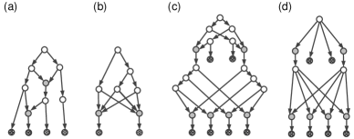
A network edge is called a reticulate edge if is a reticulate node. is tree-based if there exists a set of reticulate edges such that the subnetwork is a tree with the same set of leaves as [11], where denotes the outdegree of . Binary reticulation-visible networks are tree-based ([4, 5]). However, non-binary reticulation-visible networks may not be tree-based (Fig. 1b) [11].
Two nodes are sibling if they have a common parent. is said to be tree-sibling if every reticulate node has a sibling that is a tree node or a leaf. Note that tree-child RPNs form a subclass of tree-sibling RPNs.
3 Network Compression
3.1 Decomposition of RPNs
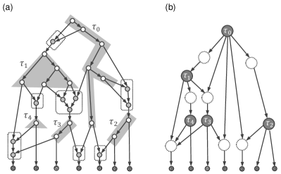
Let be an RPN over a set of taxa. Recall that and denote the sets of tree nodes and reticulate nodes, respectively. The subnetwork induced by is a forest (shaded, Fig. 2a). One connected component of the forest is a subtree rooted at the root of , whereas the rest are each rooted at the child of some reticulation. These connected components are called the tree-node components333In the papers [6, 22] that were published earlier, each tree-node component is a connected component of the forest . Here, a tree-node component contains neither leaves nor redundant nodes..
Similarly, the subnetwork induced by is also a forest. Each connected component of this forest is called a reticulation component (circled by a dashed line, Fig. 2a). It is easy to see that each reticulation component has a unique reticulate node such that any other node is above it. Such a node called the root of the component.
Proposition 3.1
Let be an RPN over such that and . Assume that contains tree-node components and reticulation components. Then,
Proof. The first inequality follows from the fact that each tree-node component is rooted at either the root of , , or the child of the lowest reticulate node of a reticulation component.
The second inequality follows from that the lowest reticulate node of every reticulation component is the parent of a leaf or the root of a tree-node component and that the tree node component rooted at is not below any reticulate node.
3.2 Compressing RPNs
Consider an RPN over a set of taxa. Recall that and denote the sets of degree-2 nodes and leaves of , respectively. Assume that contains tree-node components:
and reticulation components:
The compression of is an RPN over the same taxon set defined by:
| (1) | |||
| (2) |
where
Here, that means that is a tree (resp. reticulate) node and is a tree-node (resp. reticulation) component such that is a node in . The definition of the compression is illustrated in Fig. 2, where the network does not contain any degree-2 nodes.
For a tree (resp. reticulate) node , we use (resp. ) to denote the tree-node (resp. reticulation) component that contains . We define a surjective mapping by:
| (6) |
and a partial mapping by:
| (7) |
for any such that and . It is easy to verify that is surjective.
We further define:
| (8) | |||
| (9) | |||
| (10) |
Proposition 3.2
Let be a sub-RPN of and be .
-
(1)
is also a directed path or a node if is a directed path.
-
(2)
is connected if is connected.
-
(3)
is a tree if is a tree.
Proof. (1) Assume is a directed path (). Then, for each , by definition, or . Hence, removing identical nodes from gives a node or a directed path in .
(2) and (3) follow from Part 1.
Proposition 3.3
The compression of any tree-based RPN is also tree-based.
Proof. Assume is tree-based. Then, there exists a subset of reticulate edges such that such that is a subtree such that its leaf set is exactly equal to . For each tree-node component of , there is only one edge in such that . This edge must be in the subtree .
For each reticulation component , its nodes induce a path in . This implies that contains only one edge such that .
Taken together, by Proposition 3.2, these two facts indicate that each non-root node is of indegree 1 in the subgraph , implying that is a subtree with the leaf set in , as only the leaves of are mapped to the leaves of .
A binary RPN is galled if every reticulate node has an ancestor such that is a tree node and there are two internally disjoint paths from to in which all nodes but are each a tree node.
Theorem 3.1
Let be an RPN over a taxon set. Then,
-
(1)
is a tree if is binary and galled.
-
(2)
is a tree-child network if is reticulation-visible.
Proof. Galled networks are reticulation-visible [10]. Let be a reticulation-visible network. Let be a reticulate node of . Since is visible, by Proposition 2.1, its unique child is a visible tree node. Thus, every reticulation component contains only one reticulate node in .
(1). In an RPN, a reticulate node is inner if all its parents belong to the same tree-node component of the network. If is galled, then every reticulate node is inner [6]. For any reticulation component , we use to denote the tree-node component that contains all the parent of in . By definition, is the only parent of in . Therefore, is of indegree 1 and outdegree 1. This implies that does not contain any reticulate node and every node is of indegree 1. Thus, is a tree.
(2). Let be reticulation visible and be a tree-node component of . Since is reticulation-visible, one of the following three conditions holds: (a) contains the parent of some ; (b) contains the parent of some redundant node ; and (c) contains all the parents of a reticulate node (see [6]). If (a) (resp. (b)) holds, (resp. ) is the child of in . If Condition c holds, the node is of degree-2 and is the child of in .
Let be a redundant or reticulate node in . Since it is visible, its child must be a tree or redundant node and so has as a child. Thus, every non-leaf node has a child that is a tree or redundant node, implying that is tree-child.
4 An Application of Theorem 3.1
4.1 New network classes
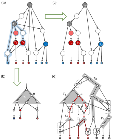
In group theory, group homomorphism and quotient group are important concepts. These concepts enable us to understand the structures of abelian groups [17, page 176]. We introduce network compression with the same spirit. It enables us to examine reticulation-visible networks from a different angle. For example, Theorem 3.1 suggests that reticulation-visible networks are networks that are expanded from tree-child network by replacing some nodes with trees. Meanwhile, the theorem can also be used to define new classes of RPNs. For instance, Fig. 2 presents a binary RPN that has a tree-child compression, but it is not reticulation-visible.
Definition 4.1
An RPN is quasi-reticulation-visible (resp. quasi-galled) if and only if is a tree-child (resp. tree) network.
4.2 Algorithm Design
The connections between clusters, trees and RPNs are basic issues in the theoretical study of phylogenetic networks. For example, different distance metrics based on clusters and trees are defined in the space of RPNs [10]. Hence, the cluster containment problem has been studied.
In a phylogenetic tree, the subset of labeled leaves below a node is called the cluster displayed at the node. Consider an RPN over and . A subset is displayed as a softwired cluster at if there is a spanning tree of in which is displayed at , where some leaves of are unlabeled non-leaf nodes of and not counted when computing a softwired cluster.
Small Cluster Containment (SCC)
Instance: An RPN over , and a tree node .
Question: Is displayed at in ?
Cluster Containment (CC)
Instance: An RPN over and .
Question: Is displayed at some node in ?
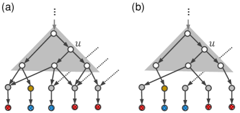
A reticulate node is isolated if neither its parents nor child is reticulate. A tree-node component is exposed if only leaves, isolated reticulate nodes and redundant nodes are found below it (Fig. 3a).
Proposition 4.1
Let be an RPN over and be a tree node in an exposed tree-node component . Then, for any , is displayed at if and only if the following two statements hold:
-
(i)
Every leaf is below , and
-
(ii)
Every leaf is not dominated by .
Proof. Assume that is displayed at in . Then, has a spanning tree in which is the cluster of . Since each leaf is below in , it is below in , implying Fact i. Since every leaf is not found below in , the path from the root to in does not contain , implying that is not dominated by in .
Conversely, assume that Facts i and ii are true. Since non-reticulate nodes below are leaves and redundant nodes only and reticulate node below are isolated, there is exactly one leaf below each reticulate node below . For a reticulate node below , we let denote its unique leaf child below and consider the following cases separately.
If is in , it is below . Hence, there is a directed path from to and then to . We then remove all reticulate edges entering that are not in .
If is not in , the fact that is not dominated by implies that there is a path from the root of to that does not contain . In this case, we also remove all reticulate edges entering that are not in the path.
After repeating the above cutting process for every reticulate node below , the subgraph below in the resulting network is a subtree containing all leaves of , implying that is a cluster of in .
In the rest of this section, we study the SCC problem on RPNs that are quasi-reticulation-visible. Let be a quasi-reticulation-visible RPN on . Without loss of generality, we may assume that does not contain any degree-2 node. By definition, is a tree-child network in which reticulate nodes are isolated and each non-leaf node is connected to some leaf by a path consisting of tree nodes and redundant nodes only. Here, we emphasize that redundant nodes are not considered to be reticulate in , although they correspond one-to-one with the reticulation components of with the property that for any two edges and such that , where is defined in Eqn. (6).
Furthermore, for determining whether is a softwired cluster at in , we just need to distinguish the leaves in from the others. Hence, we color the leaves of red and the others blue. We further extend the leaf coloring to color non-reticulate nodes that are below in . For each non-reticulate node that is below , it is colored:
-
•
Red (resp. blue) if all the non-reticulate children of are red (resp. blue).
-
•
Purple if has either at least one purple child or at least one blue child and one red child.
Since is tree-child, each non-reticulate node below will be assigned a color through this bottom-up coloring extension (Fig. 4a). It is easy to see that this coloring extension can be done in linear time. Note that and all the nodes not below have not been colored.
For each , we use:
-
•
to denote the tree-node component containing in , and
-
•
to denote the node in that represents .
Next, using the partially colored , we define a new network from , in which is exposed and there is no other tree-node component. The node set of is the union of the following node subsets:
-
1.
The tree nodes within ;
-
2.
Every leaf that is a child of in ;
-
3.
Every redundant node that is a child of in and a new leaf with the same color as ;
-
4.
Every reticulate child of in such that (i) has a blue child and (ii) the parents of are all red except , and a new leaf of blue;
-
5.
Every reticulate child of in such that (i) has a red child and (ii) does not have any red parents, and a new leaf of red.
The edge set of is the union of the following edge subsets:
-
•
The edges within ;
-
•
The reticulate edge set , where is a node added in Items 3–5 and is the reticulation component corresponding with in ;
-
•
The edges for appearing in Item 2, where is in .
-
•
The edges so that is the child of for all and are defined in Items 3–5.
How to construct is illustrated in Fig. 4. For this example, the tree-node component containing is and so in (Fig. 4a). In , has no leaf child, one redundant child and three reticulate children. The right-most reticulate child of that has a blue child has as an uncolored parent and hence does not appear in (Fig. 4b). The other three reticulate children of (shaded, Fig. 4a) appear in .
Lastly, we obtain a subnetwork of by applying the following process: For each reticulate node that is below , let be its child in .
-
•
If is red, remove all edges entering from blue and uncolored parents other than . Additionally, if has a red parent, remove also the edge from if exists.
-
•
If is blue, remove all incoming edges entering from red parents. Additionally, if has a blue or uncolored parent other than , remove also the edge from if exists.
The construction of is illustrated in Fig. 4. There are five reticulate nodes below in . The left-most one has a blue leaf as a child and has two red parents and . Hence, the edges from and to this reticulate node were removed (Fig. 4c). Similarly, we removed the edges from to the parent of , from to the parent of and from to the parent of the fourth leaf, which is red.
Proposition 4.2
Let be a quasi-reticulation-visible RPN over , and . Then, is displayed at in if and only if the following three statements hold:
-
(i)
No purple node is below in .
-
(ii)
The set of red leaves is displayed at in .
-
(iii)
is connected in which all the red leaves are below .
Proof. Assume that is displayed at in . Then, has a spanning tree in which the red leaves are exactly those below . Let and , where is the subtree of rooted at . By Proposition 3.2, is a spanning tree of and is a subtree of that contains exactly all the red leaves. For example, if is the spanning tree highlighted in red in Fig. 4d, consists of the nodes in the paths from to the three red leaves (Fig. 4c). Note that is not the subtree rooted at of in general.
If there is a purple tree node below , a red leaf and a blue leaf exist such that there are paths and from to and , respectively, that consist of non-reticulate nodes only, according to how tree nodes are colored. Clearly, and are also in , contradicting that only red leaves are found below in . This completes the proof of Fact i.
Consider a red leaf in . It represents a red leaf of or corresponds with a red node of that represents a tree-node component whose root is a dominator of a red leaf in . If the former is true, then, there is path from to . If the latter is true, there is a path from to that contains the root of in . Taken together, the two facts imply that is below in .
Consider a blue leaf in . It represents a blue leaf of or corresponds with a blue node of that represents a tree-node component whose root is a dominator of a blue leaf in . If the former is true, there is path from the root of to that avoids . If the latter is true, there is a path from the network root to that contains the root of and avoids in . This implies that is not dominated by in .
Taken together, by Proposition 4.1, the facts in the two paragraphs above imply that Fact ii is true.
Since is tree-child and is a spanning tree of , contains every path consisting of non-reticulate nodes in . Therefore, for each reticulate node below , it connects a red node with either a red node or , or it connects a blue node with a blue or uncolored node in . This implies that is subtree of . Therefore, is connected and all red leaves are below in , implying that Fact iii is true.
Conversely, assume that the three statements hold. By Fact i, no purple node is found in and hence . By Fact iii, all red leaves are below in . For each reticulate node having a red (resp. blue) child, by constrcution, is its only parent, or else its parents are all red (resp. blue or uncolored) in . Thus, any spanning tree of the subnetwork rooted at of has the following property:
In , the path from to consists of red (resp. blue) nodes (excluding ) and reticulate nodes only, for each red (resp. blue) leaf below .
This implies that a subset of red leaves is displayed at each red grandchild of by such that their union contains all the red leaves. Note that these subsets of red leaves are also displayed at the roots of the corresponding tree-node components in simultaneously.
Most importantly, by construction, each leaf of corresponds with a unique node that is either a leaf child of or a grandchild of in . Taken together, these facts and Fact ii imply that the set of all red leaves are displayed at in , as showed in Fig. 4d.
Since the three statements in Proposition 4.2 can be checked in linear time, we obtain the following resutls.
Corollary 4.1
There is a linear-time SCC algorithm for quasi-reticulation-visible networks.
Remarks The approach presented in this section can be modified to design linear-time algorithms for solving the CC problem and the tree containment problem.
5 Conclusion
We have formally introduced the concept of compression for RPNs. Using it, we have presented another interesting connection between reticulation-visible network and tree-child network and introduced a new network class for which the CC problem is solvable in linear-time. We have also showed that tree-sibling RPNs are not closed under compression, an undesired property of this network class.
We introduce network compression in analogy with quotient group in group theory. The fundamental (or basis) theorem of finite abelian groups states that every finite abelian group can be expressed as the direct product (or sum) of cyclic subgroups of prime-power order [17]. Is network compression useful for network reconstruction? This is definitely worth studying in future.
References
- [1] Cardona, G., Rosselló, F., Valiente, G.: Comparison of tree-child phylogenetic networks. IEEE/ACM Trans. Comput. Biol. Bioinform., 6, 552–569 (2009)
- [2] Cardona, G., Llabrés, M., Rosselló, F. and Valiente, G.: Metrics for phylogenetic networks I: Generalizations of the Robinson-Foulds metric. IEEE/ACM Trans. Comput. Biol. Bioinform., 6, pp.46-61.
- [3] Doolittle, W.F. and Bapteste, E.: Pattern pluralism and the Tree of Life hypothesis. Proc. Nat’l Acad. Sci., 104, 2043–2049 (2007)
- [4] Francis, A.R., Steel, M.: Which phylogenetic networks are merely trees with additional arcs? Syst. Biol. 64, 768–777 (2015)
- [5] Gambette, P., Gunawan, A.D.M., Labarre, A., Vialette, S., Zhang, L.X.: Solving the tree containment problem in linear time for nearly stable phylogenetic networks. Discrete Appl. Math., in press. https://doi.org/10.1016/j.dam.2017.07.015
- [6] Gunawan, A.D.M., DasGupta, B., Zhang, L.X.: A decomposition theorem and two algorithms for reticulation-visible networks. Inform. Comput. 252, 161– 175 (2017)
- [7] Gusfield, D.: ReCombinatorics: the Algorithmics of Ancestral Recombination Graphs and Explicit Phylogenetic Networks. MIT Press (2014)
- [8] Huber, K.T., Moulton, V., Steel, M., Wu, T.: Folding and unfolding phylogenetic trees and networks. J. Math. Biol. 73, 1761–1780.
- [9] Huson, D.H., Klöpper, T.H.: Beyond galled trees-decomposition and computation of galled networks. In: Proc. Int’l Confer. on Res. in Comput. Mol. Biol. (RECOMB), pp. 211–225. Springer (2007)
- [10] Huson, D.H., Rupp, R., Scornavacca, C.: Phylogenetic Networks: Concepts, Algorithms and Applications. Cambridge University Press (2011)
- [11] Jetten, L., van Iersel, L.: Nonbinary tree-based phylogenetic networks. IEEE/ACM Trans. Comput. Biol. Bioinform. 15, 205–217 (2018)
- [12] Kanj, I.A., Nakhleh, L., Than, C., Xia, G.: Seeing the trees and their branches in the network is hard. Theoret. Comput. Sci. 401(1-3), 153–164 (2008)
- [13] Lengauer, T., Tarjan, R.E.: A fast algorithm for finding dominators in a flowgraph. ACM Trans. Program. Lang. Syst. 1, 121–141 (1979)
- [14] Marcussen,T., et al.: Inferring species networks from gene trees in highpolyploid north american and hawaiian violets (viola, violaceae). Syst. Biol., 61, 107–126 (2012)
- [15] Moret, B.M., et al.: Phylogenetic networks: modeling, reconstructibility, and accuracy. IEEE/ACM Trans. Comput. Biol. Bioinform., 1, 13–23 (2004).
- [16] Nakhleh, L., Wang, L.S.: Phylogenetic networks: Properties and relationship to trees and clusters. In: Trans. Comput. Syst. Biol. II, pp. 82–99. Springer (2005)
- [17] Rose J.S.: A course on group theory. Dover Publications, New York, USA (2012)
- [18] Steel, M.: Phylogeny: Discrete and Random Processes in Evolution. SIAM, Philadelphia, USA (2016)
- [19] van Iersel, L., Semple, C., Steel, M.: Locating a tree in a phylogenetic network. Inform. Process. Letters 110(23), 1037–1043 (2010)
- [20] Wang, L., Zhang, K., Zhang, L.X.: Perfect phylogenetic networks with recombination. J. Comput. Biol. 8(1), 69–78 (2001)
- [21] Yan, H.Y., Gunawan, A.D.M., Zhang, L.X.: S-Cluster++: A fast program for solving the cluster containment problem for phylogenetic networks. Bioinform. (accepted) (2018).
- [22] Zhang, L.X.: Clusters, trees and phylogenetic network classes, in press.