Toward Quantitative Model for Simulation and Forecast of Solar Energetic Particles Production during Gradual Events - I: Magnetohydrodynamic Background Coupled to the SEP Model

Abstract

Solar Energetic Particles (SEPs) are an important aspect of space weather. SEP events posses a high destructive potential, since they may cause disruptions of communication systems on Earth and be fatal to crew members onboard spacecrafts and, in extreme cases, harmful to people onboard high altitude flights. However, currently the research community lacks efficient tools to predict such hazardous threat and its potential impacts. Such a tool is a first step for mankind to improve its preparedness for SEP events and ultimately to be able to mitigate their effects. The main goal of the presented research effort is to develop a computational tool that will have the forecasting capability and can be serve in operational system that will provide live information on the current potential threats posed by SEP based on the observations of the Sun. In the present paper the fundamentals of magneto-hydrodynamical (MHD) simulations are discussed to be employed as a critical part of the desired forecasting system.

1 Introduction

1.1 Potential threats of SEP

For our technologically advanced civilization, space plays an increasingly important role. The idea of interplanetary travel and even establishing colonies on Moon and Mars slowly but steadily transitions from science fiction into the realm of plausibility. However fascinating as the perspectives could sound, our ability to predict dangers that we may encounter along the way needs to be significantly improved. The dangers themselves, however, are not unknown to us. One of them comes from our Sun in the form of Solar Energetic Particles (SEP). Triggered by extreme solar events, SEP fluxes may reach values that are damaging to the electronics onboard spacecraft and potentially fatal to the crews (e.g. Joyce et al., 2015). Precedents of SEP events of such ominous scale have been recorded in the recent history.

During the Apollo program when astronauts repeatedly visited the Moon, a huge SEP event accompanied the major August 1972 solar storm. The integrated SEP flux produced by this storm could have been fatal for Moon walking astronauts since the radiation dose from energetic particles penetrating their spacesuits would have exceeded the lethal level (${\sim}400$ rems in a short period of time). Luckily, during this event the Apollo 16 astronauts were already safely back on the Earth, while the crew of Apollo 17 was still preparing for their mission. An SEP event during the historic “giant leap for mankind” lunar landing could have been fatal. NASA, and the entire world, was lucky that the Sun “cooperated” with this endeavor.

However, when planning interplanetary human missions, one cannot rely on luck. A mission to Mars and back will take several years, and there is a significant risk to have one or more extreme SEP events that “may expose the crew to doses that lead to acute radiation effects.” The fact that we cannot predict SEP events makes a human mission to Mars a “high-risk adventure” (Hellweg and Baumstark-Khan, 2007; Jäkel, 2004).

Let us come back to the Earth and consider the harmful effects of SEP events on assets at Low Earth Orbit (LEO). The terrestrial magnetic field provides some shielding for the International Space Station (ISS) as well as the majority of unmanned missions from SEPs. However, extreme SEP events, such as that of 20 January 2005 (e.g. Grechnev et al., 2008; Matthiä et al., 2009), have hard energy spectra and they are particularly rich in hundreds of MeV to several GeV protons. A significant fraction of flux of the high-energy particles, which have a high penetrating capability, can reach LEO, thus producing significant radiation hazard for human spaceflight. Comparing with the direct threat to human life and health, the SEP effect on unmanned satellites on LEO may seem to be not so important. However, the possible loss of entire satellites with their expensive computers, sensors, and other elements of electronics is not limited to the cost (typically hundreds of millions of dollars) of the satellite itself. Many satellites are integrated into vitally important systems of defense, rescue, navigation, so the disruption of such system may have catastrophic consequences.

Even closer to the Earth is the ozone (O₃) layer in the stratosphere. This layer protects the Earth against harmful solar UV and EUV emissions, and the depletion of the ozone layer would increase the number of skin cancer cases in the human population. The higher energy SEPs can reach the stratosphere. In particular, the SEP event in August 1972 reduced the ozone concentration near the North geomagnetic pole by $>20\%$, this reduction lasted for ${\sim}20$ days, i.e. well after the end of the SEP event (Heath et al., 1977). The reason is that very large SEP events can increase the ionization degree in the stratosphere by more than a factor of 100 over quiet times (see Makhmutov et al., 2009). The increased ionization initiates a chain of chemical reactions that produce so-called “odd nitrogen” molecules, like NO, which cannot be created from even nitrogen molecule, N₂. Molecules like NO catalyze the ozone decay, and each odd nitrogen molecule can “kill” millions of O₃ molecules.

Among other threats, SEP events and their increased radiation hazard make the flight routes over the North Pole more challenging, because of the increased risk of radiation exposure and interference with communication in high frequency (HF) range (Morris, 2007).

We see that some effects of extreme SEP events are only important at higher latitudes near the geomagnetic poles, approximately in the same regions where auroras are often observed. However, during relatively infrequent but more powerful events, such as the Carrington event of 1859, the aurora had been observed as far from geomagnetic poles as at Hawaii, Miami or Jerusalem (Cliver, 2006; Green et al., 2006; Green and Boardsen, 2006; Shea et al., 2006; Shea and Smart, 2006). For such events, the area in which the ozone layer is depleted may also extend well beyond the polar region and this would last longer. Air traffic may be interrupted all over the world. We know that such unique events may happen, but we do not know, how it would affect the modern technology.

These are the main reasons why SEP events are considered as one of the most important aspects of space weather. This explains the need in a predictive technology that is capable of providing a reliable quantitative forecast of SEP events and their impacts.

1.2 Mechanisms of SEP Production

First observations of “solar cosmic rays”, as SEP were referred to at the time, dated back to 1942 (see Forbush, 1946) and were immediately linked to solar flares that preceded these particles events. This hypothesis was further supported by observations that followed, and solar flares were considered to be the primary source of SEPs (Meyer et al., 1956). As number of observed events increased, it became apparent that features of events, such as the aforementioned composition, duration, etc., exhibit a wide variability (Wild et al., 1963). The discovery of Coronal Mass Ejections (CMEs) prompted formulation of a new hypothesis that SEPs are produced by interplanetary shocks that often accompany flares rather than by flares themselves (Kahler et al., 1978; Gosling, 1993).

The debate ultimately resulted in the commonly adopted paradigm (e.g. Ruffolo et al., 1998; Reames, 1999, 2002; Cliver, 2009) that states that SEP events can be divided into two distinct classes: (1) impulsive, and (2) gradual events. The former are caused by solar flares, while the latter are associated with CMEs. Gradual events are prolonged in time and more extended in longitudinal range compared to the impulsive events. Also, SEP composition was found to be a good indicator of nature of events (Cane et al., 2006), e.g. flare associated events have Fe/O abundance of ${\sim}1$ and are electron-rich, while those associated with CME-driven shocks have Fe/O abundance of  ${\sim}0.1$ and are proton-rich.

It should be noted that the pattern above was originally discovered for particles of energies that are limited by ${\sim}$30 MeV. Such particles are easily detected by instruments outside the Earth’s magnetosphere. For this reason, many models focus on this particular part of the particle population. However, the particles that pose the largest threat are those that exceed this energy, and for them the aforementioned pattern is much less clear. Based on compositional and other data, many large SEP events show signatures of both gradual and impulsive events and, thus, don’t fully agree with simple bi-modal paradigm (e.g. Cohen et al., 1999; Mazur et al., 1999). Cohen et al. (2008) explain the discrepancy by simultaneous particle producion both at flare sites and CME shock fronts, while Tylka et al. (2005) suggest that there is no true separation of events into two distinct categories: seed suprathermal particle population originates in flares and is then accelerated by CME-driven interplanetary shocks. In both of these explanations, signatures of both types of events naturally arise in large SEP events. These events are frequently associated with so-called Ground Level Events (GLEs), as most energetic particles have the potential to penetrate Earth’s magnetosphere and ionosphere (Shea and Smart, 1990, 1994, 2012; Gopalswamy et al., 2014). Relevant data are provided by measurements performed with neutron monitors. Analysis of properties of GLEs and those of associated solar flares and CMEs (e.g. Kahler et al., 2012; Gopalswamy et al., 2012) confirms that SEP production is likely to involve both types of events. Further observations, e.g. by AMS-02 instrument (Aguilar et al., 2015), will provide valuable insights into this problem. In our work, we focus primarily on gradual, shock-driven events.

Solar eruptions, including CMEs, are associated with a major restructuring of the coronal magnetic field and the ejection of solar material ($\sim$ $10^{12\div 13}$ kg) and magnetic flux ($\sim$ $10^{13\div 15}$ Wb) into interplanetary space (e.g. Roussev and Sokolov, 2006). A shock wave driven by the ejecta can accelerate charged particles to ultra-relativistic energies as the result of Fermi acceleration processes (Fermi, 1949). The diffusive-shock-acceleration (DSA) is a profound mechanism, which naturally produces the observed power-law spectra of energetic particles. It was first proposed by Krymsky (1977); Axford et al. (1977); Bell (1978a, b); Blandford and Ostriker (1978) to explain an origin of galactic cosmic rays, however, for the past four decades, this mechanism has been studied extensively also in the context of co-rotating and traveling interplanetary shocks and has been demonstrated to be well supported both by theory (e.g. Lee, 1997; Ng et al., 1999, 2003; Zank et al., 2000) and observations (e.g. Kahler, 1994; Tylka et al., 1999; Cliver et al., 2004; Tylka et al., 2005).

The most efficient particle acceleration takes place near the Sun at heliocentric distances of $2\div 15\,R_{\odot}$, and the fastest particles can escape upstream of the shock, then propagating along the lines of the interplanetary magnetic field and reaching the Earth shortly after the initiation of the CME ($\leq 1$ hr).

The theory of DSA is being debated within the community Reames (1999, 2002); Tylka (2001), since very little is known from observations about the dynamical properties of CME-driven shock waves in the inner corona soon after the onset of an eruption. The main argument against the shock origin is that near the Sun the ambient Alfvén speed is so large, due to the strong magnetic fields there, that a strongly super-magnetosonic shock wave is difficult to anticipate (Gopalswamy et al., 2001). How soon after the onset of a CME the shock wave forms, and how it evolves in time depends largely on how this shock wave is driven by the erupting coronal magnetic fields.

To address the issue of shock origin during CMEs, it is required that real magnetic data are incorporated into a global model of the solar corona, as this had been done in, for example, Roussev et al. (2004). As proposed by Tylka et al. (2005), the shock geometry plays a significant role in the spectral and compositional variability of SEPs above ${\sim}30$ MeV/nuc. Therefore, in order to explain the observed signatures of gradual SEP events, global models of solar eruptions are required to explain the time-dependent changes in the strength and geometry of shocks during these events. The CME-driven shock continues to accelerate particles, and the shock passage at 1 AU is often accompanied by an enhancement of the energetic-particle flux. To simulate this effect, the shock wave evolution should be continuously traced while it propagates to 1 AU.

1.3 Goal and content of the paper

The goal of our current and future research is to develop the computational framework embracing several coupled physical and numerical models, which could quantitatively simulate the SEP production during the gradual events with ultimately achieving a capability to predict the SEP flux and spectrum (or, at least, the probability of dangerously high flux and related radiation hazard).

In the series of two papers we outline the framework and describe its existing components. The present paper is the first in the series, it contains the review of the MHD component of the framework. The second paper will describe the kinetic component of the framework.

Some of the computational models or their couplings are still underdeveloped. Therefore, the paper mostly focuses on presenting the physical and mathematical fundamentals of the integrated model, as well as on the description of the available computational tools and their integration into the framework, rather than on the particular results of the models. Some numerical results here are provided only to illustrate operation of the models. From the brief discussion above we can summarize, which computational tools and technologies are needed to achieve the claimed research goal, therefore, what should be included into the desired computational framework.

First, one needs to simulate a full 3-D structure of the interplanetary magnetic field prior to CME, which determines the magnetic connectivity and allows simulating the SEP transport along the magnetic field lines toward 1 AU. One also needs to know the 3-D distribution of the solar wind parameters. This ambient solution affects the CME and shock wave travel time to 1 AU, hence, the time of SEP enhancement in the course of the shock wave passage. The pre-eruptive structure of the Solar Corona (SC) should also be known, since it controls the possibility for the shock wave formation at small heliocentric distances, which results in efficient DSA, as well as the magnetic connectivity of the Active Region (AR), at which CME originates, to the upper SC. To simulate the ambient solution in the SC and inner heliosphere (IH), the Alfvén wave turbulence based Solar atmosphere Model (AWSoM) is used as described in this paper in Section 2.1. In order to simulate an ongoing CME and to reach the predictive capability, the model should run faster than the Real-time, therefore, the AWSoM-R model with this feature is utilized (presented in Section 2.2). The CME-driven shock wave should be simulated starting from the lower altitude. Relevant models are described in Section 3.

The overview of MHD models and tools presented in this paper wouldn’t be complete without demonstrating how they fit into the overall framework and what makes them an irreplaceable piece in the puzzle. This requires a summary, however brief, of a particle code utilized in simulations (Section 4). We conclude the paper with the proof-of-concept results obtained with the help of our newly developed SEP forecasting framework (Section 5). Again, a detailed summary of physical models and numerical tools that will be used to describe the kinetic component of the framework are to be considered in the second paper of the series.

2 Alfvén Wave Turbulence Driven MHD Description of the Solar Corona and the Solar Wind

2.1 Steady-state solar corona and solar wind

In any predictive model for eruptive solar events, the background steady-state SC and IH are as important as a stage for a performance. If poorly designed, the foundation would compromise the whole facility. Thus, an accurate and carefully validated model for the steady-state background is vital and shouldn’t be overlooked or explored superficially. In our work we use a widely accepted paradigm that the solar wind is driven by and the SC is heated by the dissipation in, the Alfvén wave turbulence.

2.1.1 Alfvén wave turbulence

The concept of Alfvén waves was introduced more than 70 years ago by Alfvén (1942). The importance of the role they play within the Solar system was not immediately recognized due to the lack of relevant observations. Results from Mariner 2 allowed a data-backed study of a wave-related phenomena in solar wind. A detailed analysis of these observations can be found in, for example, Coleman (1966, 1967). This pioneering study culminated in Coleman (1968), a work that stated that Alfvén wave turbulence has the potential to drive solar wind in a way that is consistent with observations at 1 AU.

Attention to Alfvén waves related phenomena was continuously increasing and an ever growing number of studies on interaction of these waves with solar wind plasma and various aspects of associated effects were undertaken. Examples of the earliest efforts to investigate the role of Alfvén waves in solar wind acceleration are Belcher et al. (1969); Belcher and Davis (1971); Alazraki and Couturier (1971). A consistent and comprehensive theoretical description of Alfvén wave turbulence and its effect on the averaged plasma motion has been developed in a series of works, particularly, Dewar (1970) and Jacques (1977, 1978) (see also references therein). More recent efforts to simulate solar wind acceleration utilize the approach developed in these works (e.g. Usmanov et al., 2000). Currently, it is commonly accepted, that the gradient of the Alfvén wave pressure is the key driver for the solar wind acceleration.

At the same time, damping of Alfvén wave turbulence as a source of the coronal heating was extensively studied (e.g. Barnes, 1966, 1968). Later, it was demonstrated that reflection from the sharp pressure gradients in the solar wind (Heinemann and Olbert, 1980; Leroy, 1980) is a critical component of Alfvén wave turbulence damping (Matthaeus et al., 1999; Dmitruk et al., 2002; Verdini and Velli, 2007). For this reason, many numerical models explore the generation of reflected counter-propagating waves as the underlying cause of the turbulence energy cascade (e.g. Cranmer, 2010), which transports the energy of turbulence from the large scale motions across the inertial range of the turbulence spatial scale to short-wavelength perturbations. The latter can efficiently damp due to the wave-particle interaction. In this way, the turbulence energy is converted to the particle (thermal) energy.

Recent efforts of many studies are aimed at developing models that include Alfvén waves as a primary driving agent for both heating and accelerating of the solar wind. Examples are Hu et al. (2003); Suzuki and Inutsuka (2005); Verdini et al. (2010); Matsumoto and Suzuki (2012); Lionello et al. (2014a, b).

2.1.2 Ad Hoc Coronal Heating Functions and Semi-Empirical Models for the Solar Wind Heating

It is important to emphasize, that while incorporating the Alfvén wave driven acceleration is a matter of including the wave pressure gradient into governing equations (Jacques, 1977), there is still no widely accepted approach to describing the coronal heating via Alfvén wave turbulence cascade. A large number of models of SC heating have been constructed over the years. One can trace two major approaches to representing the process: (i) to use an ad-hoc heating function to mimic SC heating with heating rate being chosen to better fit observations; (ii) to use a semi-empirical coronal heating function that is based on aspects of physics of Alfvén waves.

The former approach is utilized, for example, by Lionello et al. (2001, 2009); Riley et al. (2006); Titov et al. (2008); Downs et al. (2010). This method provides a reasonably good agreement with observations in EUV, X-rays and white light. The agreement looks particularly impressive for the PSI predictions about the solar eclipse image (Mikić et al., 2007). An important limitation is that models utilizing an ad-hoc approach depend on a few free parameters, which need to be determined for various solar conditions. Such approach has an inherent shortcoming: although it is well-suited for typical conditions, it can’t properly account for unique conditions as those that can take place during extreme solar events.

Another illustration of the ad hoc approach is the semi-empirical model to simulate solar wind. For example, the Wang-Sheeley-Arge (WSA) model instead of incorporating physical properties of Alfvén waves, utilizes semi-empirical formulae that relate the solar wind speed with the solar magnetogram and the properties of the magnetic field lines of the potential magnetic field as recovered from the synoptic magnetogram. Its development history may be traced through Wang and Sheeley (1990, 1992, 1995); Arge and Pizzo (2000); Arge et al. (2003). The major benefit of the model is the opportunity to seamlessly integrate it into a global space weather simulation as was done in Cohen et al. (2007). In this study, the WSA formulae were used as the boundary condition for the MHD simulator via the varied polytropic gas index distribution (see Roussev et al., 2003b). Models mentioned above successfully explain observations of the solar wind parameters at 1 AU.

A number of validation and comparison studies have been published (Owens et al., 2008; Vásquez et al., 2008; MacNeice, 2009; Norquist and Meeks, 2010; Gressl et al., 2014; Jian et al., 2015; Reiss et al., 2016).

However, these models don’t fully capture the physics of Alfvén wave turbulence or even disregard it altogether. Even though some models are designed to account for the Alfvén waves’ physics Cohen et al. (such as 2007), neither does capture every aspect of the interaction of the turbulence with the background flow, which include both energy and momentum transfer from the turbulence to the solar wind plasma. Thus, neither model can be used as a fully consistent tool for simulating the solar atmosphere.

2.1.3 Alfvén-Wave-Turbulence-Based Model for the Solar Atmosphere

The ad hoc elements were eliminated from the model for the SC and quiet-time IH by Sokolov et al. (2013). In the Alfvén Wave turbulence based Solar atmosphere Model (AWSoM) the plasma is heated by the dissipation of the Alfvén wave turbulence, which, in turn, is generated by the nonlinear interaction between oppositely propagating waves (Hollweg, 1986). Within the coronal holes, there are no closed magnetic field lines, hence, there are no oppositely propagating waves. Instead, a weak reflection of the outward propagating waves locally generates sunward propagating waves as quantified by van der Holst et al. (2014). The small power in these locally generated (and almost immediately dissipated) inward propagating waves leads to a reduced turbulence dissipation rate in coronal holes, naturally resulting in the bimodal solar wind structure. Another consequence is that coronal holes look like cold black spots in the EUV and X-rays images, while the closed field regions are hot and bright, and the brightest are active regions, near which the wave reflection is particularly strong (see Sokolov et al., 2013; Oran et al., 2013; van der Holst et al., 2014).

The model equations are the following:

$$\frac{\partial\rho}{\partial t}+\nabla\cdot(\rho{\bf u})=0,$$ (2.1)

$$\frac{\partial{\bf B}}{\partial t}+\nabla\cdot\left({\bf u}{\bf B}-{\bf B}{\bf u}\right)=0,$$ (2.2)

$$\frac{\partial(\rho{\bf u})}{\partial t}+\nabla\cdot\left(\rho{\bf u}{\bf u}-\frac{{\bf B}{\bf B}}{\mu_{0}}\right)+\nabla\left(P_{i}+P_{e}+\frac{B^{2}}{2\mu_{0}}+P_{A}\right)=-\frac{GM_{\sun}\rho{\bf R}}{R^{3}},$$ (2.3)

The notation used in the equations is as follows: $\rho$ is the mass density, $\mathbf{u}$ is the velocity, $u=|{\bf u}|$, assumed to be the same for the ions and electrons, $\mathbf{B}$ is the magnetic field, $B=|{\bf B}|$, $G$ is the gravitational constant, $M_{\odot}$ is the solar mass, $\mathbf{r}$ is the position vector relative to the center of the Sun, $R=|{\bf R}|$, $\mu_{0}$ is the magnetic permeability of vacuum. As has been shown by Jacques (1977), the Alfvén waves exert an isotropic pressure (see term $\nabla P_{A}$ in the momentum equation). The relation between the wave pressure and wave energy density is $P_{A}=(w_{+}+w_{-})/2$. Herewith, $w_{\pm}$ are the energy densities for the turbulent waves propagating along the magnetic field vector ($w_{+}$) or in the opposite direction ($w_{-}$). The isotropic ion pressure, $P_{i}$, and electron pressure, $P_{e}$, are governed by the energy equations:

$$\frac{\partial}{\partial t}\left(\frac{P_{i}}{\gamma-1}+\frac{\rho u^{2}}{2}+\frac{{\bf B}^{2}}{2\mu_{0}}\right)+\nabla\cdot\left\{\left(\frac{\rho u^{2}}{2}+\frac{\gamma P_{i}}{\gamma-1}+\frac{B^{2}}{\mu_{0}}\right){\bf u}-\frac{{\bf B}({\bf u}\cdot{\bf B})}{\mu_{0}}\right\}=$$

$$=-({\bf u}\cdot\nabla)\left(P_{e}+P_{A}\right)+\frac{N_{e}N_{i}k_{B}}{\gamma-1}\left(\frac{\nu_{ei}}{N_{i}}\right)\left(T_{e}-T_{i}\right)-\frac{GM_{\sun}\rho{\bf R}\cdot{\bf u}}{R^{3}}+Q_{i},$$ (2.4)

$$\frac{\partial}{\partial t}\left(\frac{P_{e}}{\gamma-1}\right) + \nabla\cdot\left(\frac{P_{e}}{\gamma-1}{\bf u}\right)+P_{e}\nabla\cdot{\bf u}=$$ (2.5)

$$= -\nabla\cdot\mathbf{q}_{e}+\frac{N_{e}N_{i}k_{B}}{\gamma-1}\left(\frac{\nu_{ei}}{N_{i}}\right)\left(T_{i}-T_{e}\right)-Q_{\rm rad}+Q_{e},$$

where $T_{e,i}$ are the electron and ion temperatures, $N_{e,i}$ are the electron and ion number densities, and $k_{B}$ is the Boltzmann constant. Other newly introduced terms are explained below.

The equation of state $P_{e,i}=N_{e,i}k_{B}T_{e,i},$ is used for both species. The polytropic index is $\gamma=5/3$. The optically thin radiative energy loss rate in the lower corona is given by

$$Q_{\rm rad}=N_{e}N_{i}\Lambda(T_{e})$$ (2.6)

where $\Lambda(T_{e})$ is the radiative cooling curve taken from the CHIANTI version 7.1 database (Landi et al., 2013, and references therein). The Coulomb collisional energy exchange rate between ions and electrons is defined in terms of the collision frequency

$$\frac{\nu_{ei}}{N_{i}}=\frac{2\sqrt{m_{e}}L_{C}(e^{2}/\varepsilon_{0})^{2}}{3m_{p}(2\pi k_{B}T_{e})^{3/2}}$$ (2.7)

The electron heat flux $\mathbf{q}_{e}$ is used in the collisional formulation of Spitzer and Härm (1953):

$$\mathbf{q}_{e}=\kappa_{\|}\mathbf{bb}\cdot\nabla T_{e},\quad\kappa_{\|}=3.2\frac{6\pi}{\Lambda_{C}}\sqrt{\frac{2\pi}{m_{e}}\frac{\varepsilon_{0}}{e^{2}}^{2}}\left(k_{B}T_{e}\right)^{5/2}k_{B}$$ (2.8)

where $m_{e}$ and $e$ are the electron mass and charge, $m_{p}$ is the proton mass, $\varepsilon_{0}$ is the vacuum permittivity, $\mathbf{b}=\mathbf{B}/B$, $\Lambda_{C}$ is the Coulomb logarithm.

Dynamics of Alfvén wave turbulence and its interaction with the background plasma requires a special consideration. The evolution of the Alfvén wave amplitude (velocity, $\delta\mathbf{u}$, and magnetic field, $\delta\mathbf{B}$) is usually treated in terms of the Elsässer (1950) variables, $\mathbf{z}_{\pm}=\delta\mathbf{u}\mp\frac{\delta\mathbf{B}}{\sqrt{\mu_{0}\rho}}$. The Wentzel-Kramers-Brillouin (WKB) approximation is used to derive the equations that govern transport of Alfvén waves, which may be reformulated in terms of the wave energy densities, $w_{\pm}=\rho\mathbf{z}^{2}_{\pm}/4$. Dissipation of Alfvén waves, $\Gamma_{\pm}w_{\pm}$, is crucial in driving the solar wind and heating the coronal plasma. The dissipation occurs, when two counter-propagating waves interact. Therefore, an efficient source of both types of waves is needed and it is maintained by Alfvén wave reflection from steep density gradients. For this reason, we need to go beyond the WKB approximation, which assumes that wavelength is much smaller than spatial scales in the background. The equation describing propagation of the turbulence, its dissipation and reflection has been derived in van der Holst et al. (2014):

$$\frac{\partial w_{\pm}}{\partial t}+\nabla\cdot\left[(\mathbf{u}\pm\mathbf{V}_{A})w_{\pm}\right]+\frac{w_{\pm}}{2}\left(\nabla\cdot\mathbf{u}\right)=-\Gamma_{\pm}w_{\pm}\mp\mathcal{R}\sqrt{w_{-}w_{+}}.$$ (2.9)

Here, the dissipation rate equals $\Gamma_{\pm}=\frac{2}{L_{\perp}}\sqrt{w_{\mp}/\rho}$ and the reflection coefficient is given by

$${\cal R}=\min\left\{\sqrt{\left({\bf b}\cdot[\nabla\times{\bf u}]\right)^{2}+\left[({\bf V}_{A}\cdot\nabla)\log V_{A}\right]^{2}},\max(\Gamma_{\pm})\right\}\times$$

$$\times\left[\max\left(1-\frac{I_{\rm max}}{\sqrt{{w_{+}}/{w_{-}}}},0\right)-\max\left(1-\frac{I_{\rm max}}{\sqrt{{w_{-}}/{w_{+}}}},0\right)\right],$$ (2.10)

where $I_{\rm max}=2$ is the maximum degree of the turbulence “imbalance”. If $\sqrt{w\pm/w_{\mp}}<I_{\rm max}$, then ${\cal R}=0$ and the reflection term is not applied.

Now, knowing the dissipation of the Alfvén turbulence, we are able to write the expression for ion and electron heating due to turbulence

$$Q_{i}=f_{p}\left(\Gamma_{-}w_{-}+\Gamma_{+}w_{+}\right),\quad Q_{e}=(1-f_{p})\left(\Gamma_{-}w_{-}+\Gamma_{+}w_{+}\right),$$ (2.11)

where $f_{p}\approx 0.6$ is a fraction of energy dissipated to ions. Finally, to close the system of equations, we use the following boundary condition for the Poynting flux, $\Pi$:

$$\frac{\Pi}{B}=\frac{\Pi_{R_{\odot}}}{B_{R_{\odot}}}={\rm const}\approx 1.1\cdot 10^{6}\frac{\rm W}{{\rm m}^{2}{\rm T}}$$ (2.12)

The scaling law for the transverse correlation length:

$$L_{\perp}\sim B^{-1/2},\quad 100{\rm km}\cdot{\rm T}^{1/2}\leq L_{\perp}\sqrt{B}\leq 300{\rm km}\cdot{\rm T}^{1/2}$$ (2.13)

2.2 Alfvén-Wave-Turbulence-Based Model for the Solar Atmosphere in Real Time.

AWSoM has been demonstrated to be an accurate tool for modeling realistic conditions of solar wind (Sokolov et al., 2013; Oran et al., 2013; van der Holst et al., 2014). However, in terms of computational efficiency, the model is somewhat restrictive. The reason for that deficiency is the extremely fine resolution of the computational mesh close to the solar surface; such fine mesh is needed to resolve the dynamics of Alfvén wave turbulence and ensure the numerical stability. An alternative approach is to reformulate the mathematical problem in the said region. Instead of solving a computationally expensive 3-D problem on such fine grid, we substitute it with a multitude of much simpler 1-D problems along threads, that allow bringing boundary conditions up from the solar surface to a height defined by the assumptions below and are the key concept of our Threaded-Field-Line-Model (TFLM).

The main assumption in the reformulated problem is that the solar magnetic field may be considered to be potential with high accuracy in a certain range of radii, $R_{\odot}<R<R_{b}$. A thread represents a field line of such field. A 1-D problem being introduced here, concerns a flux tube that encloses the thread. Reduction from 3-D to 1-D is summarized below, for more details we refer readers to Sokolov et al. (2016). Due to the constraint on the magnetic field divergence, $\nabla\cdot\mathbf{B}=0$, the magnetic flux remains constant along the thread:

$$B(s)\cdot A(s)={\rm const},$$ (2.14)

hereafter $s$ is the distance along the field line, $B$ is the magnitude of the magnetic field, $A$ is the cross-section area of the flux tube in the consideration. Conservation laws are also greatly simplified due to the fact that in low-beta plasma, velocity is aligned with the magnetic field. Here, assuming steady-state, conservation laws take the form:

Continuity equation:

$$\frac{\partial}{\partial s}\left(\frac{\rho u}{B}\right)=0\quad\Rightarrow\quad\left(\frac{\rho u}{B}\right)={\rm const}$$ (2.15)

Conservation of momentum:

$$\quad\frac{\partial P}{\partial s}=-\frac{b_{R}GM_{\odot}\rho}{R^{2}}\quad\Rightarrow\quad P=P_{TR}e^{\int\limits_{R_{TR}}^{R}\frac{GM_{\odot}m_{p}}{2k_{B}T}d\frac{1}{R^{\prime}}},$$ (2.16)

here $R_{TR}$ is the height of the transition region (TR), $b_{R}$ is the radial component of $\mathbf{b}$ terms proportional to $u^{2}$ are neglected, $\mathbf{j}\times\mathbf{B}$ is omitted due to electric current vanishing in the potential field ($\mathbf{j}\propto\nabla\times\mathbf{B}=0$) and pressure of Alfvén wave turbulence is assumed to be much smaller than the thermal pressure, $P_{A}\ll P$.

Conservation of energy:

$$\frac{2N_{i}k_{B}}{B\left(\gamma-1\right)}\frac{\partial T}{\partial t}+\frac{2k_{B}\gamma}{\gamma-1}\left[\frac{N_{i}u}{B}\right]\frac{\partial T}{\partial s}=$$

$$\frac{\partial}{\partial s}\left(\frac{\kappa_{\|}}{B}\frac{\partial T}{\partial s}\right)+\frac{\Gamma_{-}w_{-}+\Gamma_{+}w_{+}-N_{e}N_{i}\Lambda(T)}{B}+\left[\frac{\rho u}{B}\right]\frac{\partial\left(GM_{\odot}/R\right)}{\partial s},$$ (2.17)

the term $\frac{\partial T}{\partial t}$ is retained under assumption that the electron heat conduction is a relatively slow process. Alfvén wave dynamics is reformulated as well. In Eq. 2.9 we substitute $w_{\pm}=\left[\frac{\Pi}{B}\right]\sqrt{\mu_{0}\rho}a_{\pm}^{2}$:

$$\frac{\partial a_{\pm}^{2}}{\partial t}+\nabla\cdot\left(\mathbf{u}a_{\pm}^{2}\right)\pm\left(\mathbf{V}_{A}\cdot\nabla\right)a_{\pm}^{2}=\mp\mathcal{R}a_{-}a_{+}-2\sqrt{\frac{\left[\Pi/B\right]\mu_{0}V_{A}}{\left[L_{\perp}\sqrt{B}\right]^{2}}}a_{\mp}a_{\pm}^{2}$$ (2.18)

The equations are additionally simplified since in the lower corona environment $u\ll V_{A}$, i.e. waves are assumed to travel fast and quickly converge to equilibrium, $\frac{\partial a_{\pm}^{2}}{\partial t}=0$:

$$\pm\left(\mathbf{b}\cdot\nabla\right)a_{\pm}^{2}=\mp\frac{\mathcal{R}}{V_{A}}a_{-}a_{+}-2\sqrt{\frac{\left[\Pi/B\right]\mu_{0}}{\left[L_{\perp}\sqrt{B}\right]^{2}V_{A}}}a_{\mp}a_{\pm}^{2}$$ (2.19)

Additionally, we substitute $d\xi=ds\sqrt{\frac{\left[\Pi/B\right]\mu_{0}}{\left[L_{\perp}\sqrt{B}\right]^{2}V_{A}}}$:

$$\pm\frac{da_{\pm}}{d\xi}=\mp\frac{ds}{d\xi}\frac{\mathcal{R}}{2V_{A}}a_{\mp}-a_{-}a_{+}$$ (2.20)

In order to close the system of equations we need to define the boundary conditions for TFLM. For “+” wave one needs to provide value at $\xi=\xi_{-}$, $a_{+0}$, and for “-” wave - value at $\xi=\xi_{+}$, $a_{-0}$. Specifically, at the photosphere level, as the result from Eq. 2.12 the dimensionless amplitude of the outgoing wave is equal to one: $b_{r}|_{R=R_{\odot}}>0:\,a_{+}=1\,$, $b_{r}|_{R=R_{\odot}}<0:\,a_{-}=1$. Boundary conditions at the interface between TFLM and global corona model (GCM) are:

$$\left.b_{r}\right|_{R=R_{b}}>0 : \quad\left(\frac{u}{B}\right)_{TFLM}=\quad\left(\frac{\mathbf{u}\cdot\mathbf{B}}{B^{2}}\right)_{GCM};$$

$$\quad\left(a_{-}\right)_{TFLM}=\left(a_{-}\right)_{GCM};\quad\left(a_{+}\right)_{GCM}=\left(a_{+}\right)_{TFLM}$$

$$\left.b_{r}\right|_{R=R_{b}}<0 : \quad\left(\frac{u}{B}\right)_{TFLM}=-\left(\frac{\mathbf{u}\cdot\mathbf{B}}{B^{2}}\right)_{GCM};$$ (2.21)

$$\quad\left(a_{+}\right)_{TFLM}=\left(a_{+}\right)_{GCM};\quad\left(a_{-}\right)_{GCM}=\left(a_{-}\right)_{TFLM}$$

Also one needs to sew temperature and density across the interface between TFLM and GCM. We assume that the radial component of the temperature gradient is the dominant one, then:

$$\left(\frac{\partial T}{\partial R}\right)_{GCM}=\left(\frac{\partial T}{\partial s}\right)_{TFLM}/\left|b_{R}\right|$$ (2.22)

Boundary condition for density is controlled by sign of $u$:

$${\rm for}\quad u>0 : \quad\left(\frac{N_{i}u}{B}\right)_{TFLM}=\left(N_{i}\right)_{TFLM}\left(\frac{u}{B}\right)_{GCM};$$

$${\rm for}\quad u<0 : \quad\left(\frac{N_{i}u}{B}\right)_{TFLM}=\left(\frac{N_{i}u}{B}\right)_{GCM}.$$ (2.23)

Now we close the problem by stating conditions at the lower boundary, i.e. at the top of TR. Assuming steady-state, the energy conservation equation with only dominant terms retained reads:

$$\frac{\partial}{\partial s}\left(\kappa_{0}T^{5/2}\frac{\partial T}{\partial s}\right)=N_{e}N_{i}\Lambda(T),$$ (2.24)

where $\kappa_{\|}=\kappa_{0}T^{5/2}$.

For a chosen width of TR along the field line, $L_{TR}=\int\limits_{r_{\odot}}^{r_{TR}}ds$, and for a given temperature on top of the TR, $T_{TR}$, one can solve the heat flux and pressure from the following equations:

$$[N_{i}k_{B}T] = \frac{1}{L_{TR}}\int_{T_{ch}}^{T_{TR}}{\frac{\kappa_{0}\tilde{T}^{5/2}d\tilde{T}}{U_{\rm heat}(\tilde{T})}}$$

$$\kappa_{0}T_{TR}^{5/2}\left(\frac{\partial T}{\partial s}\right)_{T=T_{TR}} = [N_{i}k_{B}T]U_{\rm heat}(T_{TR})$$ (2.25)

$\Lambda(T)$ and $U_{\rm heat}(T)=\sqrt{\frac{2}{k_{B}^{2}}\int^{T}_{T_{ch}}{\kappa_{0}(T^{\prime})^{1/2}\Lambda(T^{\prime})dT^{\prime}}}$ are easy to tabulate using CHIANTI database, $T_{ch}\approx(1\div 2)10^{4}K$.

Thus, TFLM is fully described as a closed mathematical problem that can be solved numerically.

3 CME Models in Numerical Simulations

As mentioned above, we focus in our work on gradual SEP events. Events of this kind are characterized by a steadily increasing particle flux, unlike impulsive events, which have an abrupt time profile (Reames, 1999). Based on numerous observations (Kahler et al., 1978), it is commonly accepted that gradual, proton-rich SEP events are associated with CMEs. The two phenomena are linked via interplanetary shock wave, which forms in front of a CME: the shock wave itself results from interaction of a CME with ambient solar wind plasma and at the same time, as shock moves outwards, it accelerates more and more particles, hence the gradual nature of events.

Thus, properties of gradual SEP events are strongly influenced by CMEs that trigger them. Therefore, in order to successfully design a predictive model for gradual SEP events, we need an accurate model to describe CMEs. Due to the lack of in-situ measurements of the shock waves and the excited turbulence in their vicinity, numerical simulations remain the primary means of research. A series of numerical studies employing the theory of DSA were performed in cases of both idealized (Zank et al., 2000; Rice et al., 2003; Li et al., 2003) and realistic (Sokolov et al., 2004; Kóta et al., 2005) CME-driven shock waves.

While there are many models of CME initiation by magnetic free energy, these simulations are often performed in a small Cartesian box (e.g. Török and Kliem, 2005), or using global models with no solar wind (e.g. Antiochos et al., 1999; Fan and Gibson, 2004). So far, there have only been a few magnetically driven Sun-to-Earth CME simulations through a realistic interplanetary medium using 3-D MHD (see Manchester et al., 2004b, 2005; Lugaz et al., 2007; Tóth et al., 2007). The MHD simulation of Tóth et al. (2007) was able to match the CME arrival time to Earth within 1.8 hours and reproduce the magnetic field magnitude of the event.

In general, the purpose of a CME generator is to enhance locally the free magnetic energy of the existing global (”ambient”) solution describing the steady state of the SC and IH magnetic field, ${\bf B}_{\rm amb}({\bf R})$, by superposing an erupting configuration representing a CME’s ejecta. A choice of a reasonable representation of the latter is still debatable. A simple but convenient way to simulate a magnetically-driven CME is to superimpose magnetic flux-rope configuration onto the background state of the SC. Such magnetic configuration describes an erupting magnetic filament filled with a plasma of excessive density. That filament becomes an expanding flux rope (magnetic cloud) in the ambient solar wind while evolving and propagating outward from the Sun, thus allowing the simulation of the propagation to 1 AU of a magnetically driven CME. In this paper, we provide a brief discussion of several approaches to generate CMEs with this technique.

3.1 Magnetized cone model

Observations of halo CMEs (e.g. with LASCO instrument, Brueckner et al., 1995; Plunkett et al., 1998) provided new insights into the geometry of CMEs and its relation with other properties. One can accurately infer the angular width and the central position angle of a halo CME together with the plasma velocity. For example, these observations have revealed that: (i) the bulk velocity tends to be radial; (ii) the angular width, $2\Delta\theta$, tends to remain constant as CME propagates through the corona. These persistent features lead to the development of the cone model (Zhao et al., 2002). Having only three free parameters, angular width of a CME and its initial position on the solar surface, the model approximates a CME and its propagation with a cone with apex located at the center of the Sun. It was later improved by Michalek (2006) for arbitrary shapes. The cone model is successfully used at Community Coordinated Modeling Center (CCMC) and has proved to be an efficient tool for predicting arrival times of CMEs (Vršnak et al., 2014; Mays et al., 2015). Thanks to the model’s accuracy and robustness, it is used together with WSA model in CCMC’s operational activities. However, by design, the cone model lacks details about the magnetic field carried by a CME. The model may be substantially enriched as we suggest below.

In order for the simulated CME ejecta to truly represent a magnetic cloud, one needs to incorporate magnetic field, controlled by the ambient external field at the location where CME is added, into the model. One possible way to achieve this is to impose a spheromak, i.e. an equilibrium spherical MHD configuration (see Appendix A), around the central point of the cloud, ${\bf R}_{\rm c}$. Spheromak’s magnetic field is:

$${\bf B}_{\rm sk}({\bf r})=\left[\frac{j_{1}({\alpha_{0}}{r})}{\alpha_{0}{r}}-\beta_{0}\right]\left(2{\bf B}_{0}+\sigma_{h}\alpha_{0}[{\bf B}_{0}\times{\bf r}]\right)+j_{2}(\alpha_{0}{r})\frac{[{\bf r}\times[{\bf r}\times{\bf B}_{0}]]}{r^{2}},$$ (3.1)

where $j_{1}$ and $j_{2}$ are spherical Bessel functions. Herewith, the vector ${\bf B}_{0}$ is introduced with the magnitude equal to $B_{0}$ directed along spheromak’s axis of symetry, $\sigma_{h}=\pm 1$ is the sign of helicity (we assume $\alpha_{0}={\rm const}>0$), $\beta_{0}={\rm const}$ is the charactersitic value of plasma beta. The coordinate vector, ${\bf r}$, originates at the center of configuration, $\mathbf{R}_{\rm c}$. We assume no currents outside a spherical magnetic surface $\|{\bf R}-{\bf R}_{\rm c}\|=r_{0}$, which thus bounds the configuration. The radial and toroidal components of the magnetic field turn to zero at the surface, thus $j_{1}(\alpha_{0}r_{0})=\beta_{0}\alpha_{0}r_{0}$. For a given $\beta_{0}$ this equation relates the configuration size, $r_{0}$, to the extent of magnetic field twisting, $\alpha_{0}$, needed to close the configuration within this size.

One also needs to account for the field, which the currents inside spheromak produce outside the boundary, $\|{\bf R}-{\bf R}_{\rm c}\|=r_{0}$. The calculation of the magnetic moment (see definition in Jackson, 1999), $\mathfrak{m}$, of the spheromak configuration gives:

$$\mathfrak{m}=\frac{1}{2}\int\limits_{\|{\bf r}\|\leq r_{0}}{d^{3}r[{\bf r}\times{\bf j}]}=\frac{1}{2\mu_{0}}\int\limits_{\|{\bf r}\|\leq r_{0}}{d^{3}r[{\bf r}\times[\nabla\times{\bf B}_{\rm sk}]]}=\frac{4\pi r_{0}^{3}}{3\mu_{0}}j_{2}({\alpha_{0}r_{0}}){\bf B}_{0}$$ (3.2)

The final expression for $\mathfrak{m}$ is obtained via reducing the volume integral to the integral over the spheromak’s surface, at which ${\bf B}_{\rm sk}|_{r=r_{0}}=j_{2}(\alpha_{0}r_{0})\frac{[{\bf r}\times[{\bf r}\times{\bf B}]]}{r^{2}}$. The field of magnetic dipole, $\mathfrak{m}$, which we admit as the spheromak’s field outside the boundary, equals:

$${\bf B}_{{\rm sk,}r>r_{0}}({\bf r})=\frac{\mu_{0}}{4\pi r^{3}}\left\{\frac{3\left({\bf r}\cdot\mathfrak{m}\right){\bf r}}{r^{2}}-\mathfrak{m}\right\}=j_{2}({\alpha_{0}r_{0}})\frac{r_{0}^{3}}{r^{3}}\left\{\frac{\left({\bf r}\cdot{\bf B}_{0}\right){\bf r}}{r^{2}}-\frac{{\bf B}_{0}}{3}\right\}$$ (3.3)

Now, we provide the full expression for a spheromak superposed onto ambient field, $B_{\rm amb}(\mathbf{r})$ :

$${\bf B}({\bf R})=\left\{\begin{array}[]{c}{\bf B}_{\rm amb}({\bf R})+{\bf B}_{{\rm sk,}r>r_{0}}({\bf R}-{\bf R}_{\rm c}),\quad\|{\bf R}-{\bf R}_{\rm c}\|\geq r_{0}\\ \left[{\bf B}_{\rm amb}({\bf R})+\frac{2}{3}j_{2}({\alpha_{0}r_{0}}){\bf B}_{0}\right]+{\bf B}_{\rm sk}({\bf R}-{\bf R}_{\rm c}),\quad\|{\bf R}-{\bf R}_{\rm c}\|\leq r_{0}\end{array}\right.$$ (3.6)

where the uniform field, $\frac{2}{3}j_{2}({\alpha_{0}r_{0}}){\bf B}_{0}$ is added to the spheromak field for two reasons. First, this preserves the field continuity at $\|{\bf R}-{\bf R}_{\rm c}\|=r_{0}$, i.e. from both side of the boundary the field equals $j_{2}({\alpha_{0}r_{0}})\left\{\frac{\left({\bf r}\cdot{\bf B}_{0}\right){\bf r}}{r^{2}}-\frac{{\bf B}_{0}}{3}\right\}$. Second, certain aspects of CME ejecta’s interaction with ambient plasma dictate this correction. Indeed, if an ejecta represents a magnetic cloud, its frozen in magnetic field effectively replaces the pre-existing field, $\mathbf{B}_{\rm amb}$, at any location, $\mathbf{R}_{\rm cloud}$, it passes. Therefore,the cloud’s internal field, which we assume to be the superposition of the ambient field with the field of the spheromak centered at $\mathbf{R}_{\rm cloud}$ (i.e. $\mathbf{R}_{\rm cloud}\equiv\mathbf{R}_{\rm c}$), must be corrected by the negative of this pre-existing field. This reasoning demands the expression in the square brackets in Eq. 3.6 be exactly zero at $\mathbf{R}_{\rm c}$, i.e. $\mathbf{B}_{0}$ and $\mathbf{B}_{\rm amb}$ must be related as:

$${\bf B}_{0}=-\frac{3}{2j_{2}(\alpha_{0}r_{0})}{\bf B}_{\rm amb}({\bf R}_{\rm c})$$ (3.7)

which ensures both the continuity of the field, Eq. 3.6, and the proximity of the internal field (equality, if the ambient field is uniform), $\left[{\bf B}_{\rm amb}({\bf R})-{\bf B}_{\rm amb}({\bf R}_{\rm c})\right]+{\bf B}_{\rm sk}({\bf R}-{\bf R}_{\rm c})$, to the equilibrium state ${\bf B}_{\rm sk}({\bf R}-{\bf R}_{\rm c})$. Should the field of the superimposed configuration not match the ambient field in direction, the non-zero torque, $\left[\mathfrak{m}\times{\bf B}_{\rm amb}({\bf R}_{\rm c})\right]$ acting on the magnetic moment, $\mathfrak{m}$, in the field ${\bf B}_{\rm amb}({\rm R}_{\rm c})$, would tend to align the configuration axis with the external field. Should the configuration field be stronger/weaker than that governed by Eq. 3.7, the ambient field would be too weak/strong to balance the hoop force in the spheromak configuration, so that the latter would tend to expand/shrink. The field in the configuration determined by Eqs. 3.6, 3.7 is oppositely directed and somewhat stronger than the ambient field. For comparison, the field in the center of configuration equals: ${\bf B}_{\rm sk}({\bf R}_{\rm c})=2(\frac{1}{3}-\beta_{0}){\bf B}_{0}=-\frac{1-3\beta_{0}}{j_{2}(\alpha_{0}r_{0})}\mathbf{B}_{\rm amb}(\mathbf{R}_{\rm c})$. Magnetic geometry of the described configuration provides a natural explanation of the geomagnetic activity caused by CMEs. Indeed, if the configuration described above passes the Earth location, the local magnetic field may consequently change from ${\bf B}_{\rm amb}({\bf R}_{\rm c})$ to ${\bf B}_{\rm sk}({\bf R}_{\rm c})$ and back, so that all components of the interplanetary magnetic field change sign and increase in absolute value by a factor of $\frac{(1-3\beta_{0})}{j_{2}(\alpha_{0}r_{0})}\approx(4\div 5)$. This is a classical scenario for the magnetospheric storm.

Disregarding the solar gravitational pull and assuming uniform ambient field, the magnetic configuration described above is in a force equilibrium. As demonstrated by Low (1982), once some special distribution of plasma velocity is imposed onto an equilibrium magnetic structure with adiabatic index $\gamma{=}4/3$ , this structure starts to evolve self-similarly, i.e. with the only change in its geometry being the radial motion and uniform expansion (see Sedov, 1959; Zel’dovich and Raizer, 1967, about self-similar solutions). Specifically, we need to assume, and implement in the numerical simulations, the radially diverging initial motion with the radial velocity at each point being proportional to the heliocentric distance:

$$\mathbf{u}|_{t=0}=U_{\rm CME}\frac{\mathbf{R}}{\|\mathbf{R}_{\rm c}\|},$$

where the CME speed, $U_{\rm CME}$, may be found from observations. In application to the magnetized cone model this means that superimposing a spheromak with such velocity profile onto a barometric atmosphere would be consistent with basic principles of the cone model of Zhao et al. (2002): (i) bulk velocity of the resulting magnetic cloud is radial, and (ii) shape of the cloud, due to self-similarity, remains constant. As noted above, we neglected the gravity, i.e. the moving magnetic cloud isn’t in the perfect force equilibrium. Therefore, exact self-similarity can’t be achieved, rather it is approached when relative contribution of gravitational force tending to decelerate the cloud is small. Another force tending to decelerate the magnetic cloud is the drag force, which opposes to the faster CME motion through the slower moving ambient. On the other hand, in non-uniform ambient magnetic field anti-parallel to $\mathbf{B}_{0}$, the force acting on the magnetic dipole, repels it out of the active region, thus, accelerates its radial motion. These counteracting forces may partially balance each other, thus resulting in almost steady radial motion as assumed by the cone model.

3.2 Stretched Spheromak Configuration by Gibson-Low

The family, (3.1), of equilibrium configurations may be extended with the use of coordinate transformation suggested by Gibson and Low (1998). The arising pressure imbalance perfectly compensates the gravitational force acting on the spheromak’s plasma. The new equilibrium configuration in the heliocentric coordinates, $\mathbf{R}$, with the magnetic field, $\mathbf{B}(\mathbf{R})$, and pressure distribution, $P(\mathbf{R})$, may be described in terms of the spheromak solution, (3.1), of the Grad-Shafranov equations (see Appendix A), ${\bf B}^{\prime}({\bf R}^{\prime})=\mathbf{B}_{\rm sk}(\mathbf{R}^{\prime}-\mathbf{R}_{\rm c})$ and $P^{\prime}({\bf R}^{\prime})=P_{\rm sk}(\mathbf{R}^{\prime}-\mathbf{R}_{\rm c})$. For each point, $\mathbf{R}$, we take the values of these functions in the point, $\mathbf{R}^{\prime}(\mathbf{R})=\left(1+\frac{a}{R}\right)\mathbf{R}$, $R^{\prime}=R+a$, which is radial coordinate stretching, an arbitrary constant $a$ being the distance of stretching. When the stretching transformation is applied, it displaces the magnetic configuration toward the heliocenter and gives it a teardrop-like shape. The magnetic field vector in the course of stretching should be scaled in addition to the coordinate transformation:

$$\mathbf{B}(\mathbf{R})=\frac{R^{\prime}}{R}\left(\mathbb{I}+\frac{a}{R}\mathbf{e}_{R}\mathbf{e}_{R}\right)\cdot\mathbf{B}^{\prime}(\mathbf{R}^{\prime})$$ (3.8)

where $\mathbf{e}_{R}=\mathbf{R}/R$ and $\mathbb{I}$ is the identity matrix. The radial field component, $B^{\prime}_{R}=\left(\mathbf{B}^{\prime}\cdot\mathbf{e}_{R}\right)$, is thus multiplied by $\left(\frac{R^{\prime}}{R}\right)^{2}$, all the other by $\frac{R^{\prime}}{R}$. Thus transformed magnetic field is divergence-free. The plasma pressure of the stretched magnetic configuration is defined as:

$$P(\mathbf{R})=\left(\frac{{R^{\prime}}}{R}\right)^{2}\left(P^{\prime}-\frac{a}{R}\left(2+\frac{a}{R}\right)\frac{B^{\prime\,2}_{R}}{2\mu_{0}}\right)$$ (3.9)

One can verify an equilibrium condition for the transformed magnetic configuration. The spatial derivatives of $\mathbf{B}^{\prime}(\mathbf{R}^{\prime})$ and $P^{\prime}(\mathbf{R}^{\prime})$ are transformed as follows: $\nabla=\left[\left(1+\frac{a}{R}\right)\mathbb{I}-\frac{a}{R}\mathbf{e}_{R}\mathbf{e}_{R}\right]\cdot\nabla^{\prime}$. Using the equilibrium condition for a non-stretched configuration, $\frac{1}{\mu_{0}}[[\nabla^{\prime}\times\mathbf{B}^{\prime}]\times\mathbf{B}^{\prime}]-\nabla^{\prime}P^{\prime}=0$, the left hand side of Eq. A1 may be reduced to the following form: $\frac{1}{\mu_{0}}\left[\left[\nabla\times\mathbf{B}\right]\times\mathbf{B}\right]-\nabla P=F_{R}\mathbf{e}_{R}$, where the radial force arising from extra tension of the stretched magnetic field is:

$$F_{R}=\frac{{a}R^{\prime\,2}}{R^{3}}\left[\left({2}+\frac{a}{R}\right)\left(\frac{B^{\prime\,2}}{\mu_{0}R^{\prime}}+\left(\mathbf{e}_{R}\cdot\nabla^{\prime}\right)\left(P^{\prime}+\frac{B^{\prime\,2}}{2\mu_{0}}\right)\right)+\frac{2P^{\prime}}{R^{\prime}}-\left(3+2\frac{a}{R}\right)\frac{B^{\prime\,2}_{R}}{\mu_{0}R}\right]$$ (3.10)

Now, one can consider the stretched magnetic configuration described by Eqs. 3.8,  3.9 once superposed with some background barometric distribution of pressure, $P_{\rm bar}(\mathbf{R})$, and density, $\rho_{\rm bar}(\mathbf{R})$, which satisfy the hydrostatic equilibrium condition, $-\nabla P_{\rm bar}+\rho_{\rm bar}\mathbf{g}=0$, $\mathbf{g}=-GM_{\odot}\mathbf{e}_{R}/R^{2}$. The superposed distribution satisfies the equilibrium condition accounting for gravity:

$$\frac{1}{\mu_{0}}\left[\left[\nabla\times\mathbf{B}\right]\times\mathbf{B}\right]-\nabla\left(P+P_{\rm bar}\right)+\left(\rho+\rho_{\rm bar}\right)\mathbf{g}=0$$ (3.11)

if the density variation due to the effect of stressed field is

$$\rho=\frac{F_{R}}{g(R)}$$ (3.12)

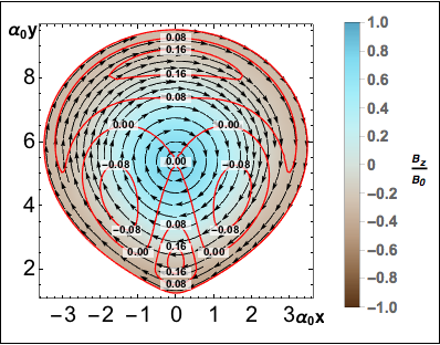
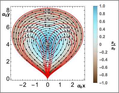
Figure 1: Equatorial plane of the stretched flux rope for $\beta_{0}{=}0.02$ (cf. Fig. 5). The original flux rope is shifted by distance $1.6r_{0}$ along a direction in the equatorial plane and then stretched towards the heliocenter by distance $0.3r_{0}$ (left) and $0.6r_{0}$ (right). Magnetic field direction is marked with arrows, off-plane component of the magnetic field is normalized per $B_{0}$ (see Eq. 3.1) and shown by color. Local values of plasma parameter $\beta({\bf r})=\mu_{0}P({\bf r})/B^{2}({\bf r})$ are shown with red curves corresponding to levels $\beta=0.04,0.08,0.12,0.16$ as marked explicitly.

As a result of the transformation, the spherical configuration is stretched towards the heliocenter as shown in Fig. 1. When the solution represented by Eq. 3.8, 3.9, 3.12 (the GL flux rope) is superimposed onto the existing corona, the sharper end of the teardrop shape is submerged below the solar surface. In the wider top part of the configuration (”balloon”) the density variation in Eq. 3.12 is negative, that is the resulting density is lower than that of the ambient barometric background. As the result, the Archimedes force acting on this part pulls the whole configuration outward the Sun. The cavity with the reduced density is often observed in the CME images from the LASCO coronagraphs. Then, in the narrower bottom part of the configuration (”basket”) the excessive positive density simulates the dense ejecta, which is pulled outward the Sun by the radial tension in the stretched magnetic configuration. Finally, the tip of the configuration with the magnetic field lines both ingoing and outgoing the solar surface in anchored to the negative and positive magnetic spots of a bipolar AR, considered as the source of the CME. Depending on the reconnection rate, the configuration can either keep being magnetically connected to the AR, or it may disconnect and close and then propagate toward 1 AU as the magnetic cloud.

The time evolution of GL flux rope is self-similar (provided $\gamma=4/3$, see Low, 1982). Additionally, this result may be generalized: adjusting the density profile in Eq. 3.12 for effective gravity $g(R)+\alpha R$ would result in accelerated/decelerated propagation of a CME. A literal requirement for self-similarity of GL flux rope can hardly be fulfilled in realistic corona. Indeed, in order for the configuration to remain in force-equilibrium (or to keep the specific shape of the force imbalance to maintain acceleration) and therefore propagate in a self-similar fashion, a specific and unrealistic distribution of the external pressure is needed. Additionally, since the Ampere’s force is non-linear in magnetic field, superimposing GL flux-rope adds a new effect of the background magnetic field onto the flux-rope’s currents, which contributes even more to the force imbalance. The significance of these effects hasn’t been thoroughly studied, however, CME propagation has been shown to be approximately self-similar (e.g. Manchester et al., 2004a, b).

The GL flux rope model has been used for CME initiation in, for example, Manchester et al. (2004a, b, 2006); Lugaz et al. (2005); Jin et al. (2017a, b). The recent developments allowed significant simplification of the process of triggering CMEs using GL model. The product of the effort is the Eruptive Event Generator based on Gibson-Low magnetic configuration (EEGGL) (Jin et al., 2017b), which is discussed in details in Borovikov et al. (2017).

3.3 Thin Flux Rope by Titov-Demoulin

The approach of TD also stems from consideration of the magnetic field’s topology. A pre-eruptive configuration of the field is reconstructed with 3 different components, $\mathbf{B}_{I}$, $\mathbf{B}_{q}$, $\mathbf{B}_{\theta}$. $\mathbf{B}_{I}$ is created by a uniform ring current flowing in the emerging flux rope (later the model has been modified in Titov et al. (2014) to include a non-uniform current profile, TDm hereafter), $\mathbf{B}_{q}$ is the magnetic field of two equal imaginary magnetic charges of opposite signs embedded below the solar surface and, finally, $\mathbf{B}_{\theta}$ is produced by a constant line current flowing through the said charges.

The TD flux rope model has been used in a number of studies (Roussev et al., 2003a; Manchester et al., 2008, e.g.), as well as its modified version, TDm (Linker et al., 2016). Specific examples of CME simulations using the AWSoM model for the SC and IH with a superimposed TD magnetic configuration include Manchester et al. (2012) and Jin et al. (2013).

4 Interface between MHD and Kinetic Models

4.1 Transport equation

The transport of energetic particles through the inter-planetary space by itself is an important problem in space science. It was studied since the discovery of the Galactic Cosmic Rays (GCR), the energetic particles originating from beyond the Solar system. A comprehensive summary of the problem can be found in the review by Parker (1965). Although results in the said review are obtained in a different context, some can readily be applied for the SEP transport.

The distribution of SEPs is far from Maxwellian, therefore, they should be characterized by a (canonical) distribution function $F({\bf R},{\bf p},t)$ of coordinates, ${\bf R}$, and momentum, ${\bf p}$, as well as time, $t$, such that the number of particles, $dN$, within the elementary volume, $d^{3}{\bf R}$, is given by the following integral: $dN=d^{3}{\bf R}\int{d^{3}{\bf p}\,F({\bf R},{\bf p},t)}$. In a magnetized plasma, it is convenient to deal with the distribution function at the given point, ${\bf R}$, in the co-moving frame of reference, which moves with the local speed of interplanetary plasma, ${\bf u}({\bf R},t)$, on introducing spherical coordinates, $(p=|{\bf p}|,\mu={\bf b}\cdot{\bf p}/p,\varphi)$ in the momentum space with its polar axis aligned with the direction of the magnetic field, ${\bf b}$, herewith $\mu$ being the cosine of pitch-angle. The normalization integral in these new variables becomes: $dN=d^{3}{\bf R}\int_{0}^{\infty}{p^{2}dp\int_{-1}^{1}{d\mu\int_{0}^{2\pi}{d\varphi F({\bf R},p,\mu,\varphi,t)}}}$. Using this canonical distribution function, one can also define a gyrotropic distribution function, $f({\bf R},p,\mu,t)=\frac{1}{2\pi}\int_{0}^{2\pi}{d\varphi F({\bf R},p,\mu,\varphi,t)}$. This function is designed to describe the particle motion averaged over the phase of its gyration about the magnetic field. The isotropic (omnidirectional) distribution function, $f_{0}({\bf R},p,t)=\frac{1}{2}\int_{-1}^{1}{d\mu f({\bf R},p,\mu,t)}$ is averaged over the pitch angle too. The normalization integrals are: $dN=2\pi d^{3}{\bf R}\int_{0}^{\infty}{p^{2}dp\int_{-1}^{1}{d\mu f({\bf R},p,t)}}=4\pi d^{3}{\bf R}\int_{0}^{\infty}{p^{2}dpf_{0}({\bf R},p,t)}$

The commonly used kinetic equation for the isotropic part of the distribution function has been introduced in Parker (1965):

$$\frac{\partial}{\partial t}f_{0}\left(\mathbf{R},p,t\right)+\left(\mathbf{u}\cdot\nabla\right)f_{0}\left(\mathbf{R},p,t\right)-\frac{1}{3}\left(\nabla\cdot\mathbf{u}\right)\frac{\partial}{\partial\ln p}f_{0}\left(\mathbf{R},p,t\right)=\nabla\cdot\left(\kappa\cdot\nabla f_{0}\left(\mathbf{R},p,t\right)\right)+S,$$ (4.1)

where $\varkappa=D_{xx}\mathbf{b}\mathbf{b}$ is the tensor of parallel (spatial) diffusion along the magnetic field, $S$ is the source term. In this approximation, the cross-field diffusion of particles is neglected.

Eq. 4.1 captures the effect of interplanetary plasma and IMF on the SEP transport and acceleration. The term proportional to the divergence of $\mathbf{u}$ is the adiabatic cooling, for $\left(\nabla\cdot\mathbf{u}\right)>0$, or (the first order Fermi) acceleration in compression or shock waves. According to estimates by Parker (1965), during quiet time the adiabatic scaling of particles’ energy from their origin to 1 AU is $\propto\left(\rho_{1AU}/\rho_{\odot}\right)^{\left(n/3\right)}$, where $n{=}2$ for non-relativistic and $n{=}1$ for relativistic particles.

Small scale irregularities also have a significant impact on particle propagation. Their scale is ${\sim}10^{5}{\div}10^{7}$ km, which is comparable with gyroradii of SEP but very small compared to 1 AU. Particles scatter on these irregularities, and on the large scale the particle motion can be described as diffusion, the first term on the right in Eq. 4.1. Based on Eq. 4.1, Krymsky (1977); Axford et al. (1977); Bell (1978a, b); Blandford and Ostriker (1978) proposed the (DSA) mechanism to explain the observed power-law spectra of GCRs.

In the present paper we limit our consideration with the case of the Parker equation 4.1 as the model to describe the SEP acceleration and transport. More realistic and accurate models accountic for the pitch-angle dependence for the distribution function are delegated to the companion paper.

4.2 Lagrangian coordinates and Field Line Advection Model

We adopt Eq. 4.1 as mathematical approach to the problem of SEP transport. However, this consideration is computationally challenging: a fully 3-D propagation of particles requires significant resources. This can be avoided by observing that Eq. 4.1 assumes that the particle motion in physical space consists of the particle guiding center’s displacement along the interplanetary magnetic field (IMF) and advection with plasma into which the IMF is frozen. This property allows us to describe the particle propagation in the Lagrangian coordinates. The benefits of this approach is the reduction of a complex 3-D problem to a multitude of much simpler 1-D problems along magnetic field lines, with no loss of generality.

At the early age of the mechanics of continuous media there were two competing approaches to a mathematical description of the motion of fluids. In Eulerian coordinates, ${\bf R},t$, the distribution of the fluid parameters (density, velocity, temperature, pressure, etc) at each instant of time, $t$, is provided as a function of coordinates, ${\bf R}$, in some coordinate frame. No need to emphasize that the any given point, ${\bf R}$ is immovable, while the fluid passes this point with the local flow velocity ${\bf u}({\bf R},t)$, so that at each time instant the fluid element at this point differs from that present at this point a while ago. In contrast with this approach, the Lagrangian coordinates, ${\bf R}_{L}$, stay with the given fluid element rather than with the given position in space. While the fluid moves, each moving fluid element keeps unchanged the value of the Lagrangian coordinates, ${\bf R}_{L}$, while its spatial location, ${\bf R}\left({\bf R}_{L},t\right)$, changes in time in accordance with the definition of the local fluid velocity:

$$\frac{D{\bf R}({\bf R}_{L},t)}{Dt}={\bf u}({\bf R},t)$$ (4.2)

Here, the partial time derivative at constant Lagrangian coordinates, ${\bf R}_{L}$ is denoted as $\frac{D}{Dt}$, while the usual notation, $\frac{\partial}{\partial t}$, denotes the partial time derivative at constant Eulerian coordinates, ${\bf R}$. As usually, we choose the Lagrangian coordinates for a given fluid element equal to the Eulerian coordinates of this element at the initial time instant, ${\bf R}_{L}={\bf R}|_{t=0}$. For numerical simulations, with any choice of the grid in Lagrangian coordinates, $\left({\bf R}_{ijk}\right)_{L}=\left({\bf R}_{ijk}\right)|_{t=0}$, one can numerically solve the multitude of ordinary differential equations, Eq. 4.2, to trace the spatial location for all Lagrangian grid points in the evolving fluid velocity field, ${\bf u}({\bf R},t)$, as long as the latter is known.

An example of application of Lagrangian coordinates to the Parker equation, Eq. 4.1, is FLAMPA (Sokolov et al., 2004).

4.3 M-FLAMPA

Geometry of magnetic field lines may become very complex and they can form intricate patterns as they evolve in time. By pushing and twisting field lines, extreme events, such as CMEs and associated interplanetary shocks, can make the field line topology even more complex. This makes forecasting the regions affected by SEP events a challenging problem. To address this challenge one needs to design a computational technique that naturally and efficiently describes this ever evolving geometry. The Multiple-Field-Line-Advection Model for Particle Acceleration (M-FLAMPA) code was designed to solve this problem. M-FLAMPA allows us to solve the kinetic equation for SEPs along a multitude of interplanetary magnetic field lines originating from the Sun, using time-dependent magnetic field and plasma parameters obtained from the MHD simulation. The model is a high-performance extension of the original FLAMPA code (Sokolov et al., 2004), which simulates SEP distribution along a single field line. M-FLAMPA is a major improvement that takes full advantage of modern supercomputers.

M-FLAMPA solves for gyrotropic SEP distribution function $f(\mathbf{x},p,t)$, where $p$ is the magnitude of the relativistic momentum of energetic particles. The code takes advantage of the fact that particles stay on the same magnetic field line and, therefore, the distribution function may be treated as a function of the distance along the filed line, $s$, rather than a 3-D vector $\mathbf{x}$. Also, coefficients in the governing equations depend only on background plasma parameters and their Lagrangian derivatives (see Section 4.2). This important property reduces the problem of particle acceleration in 3-D magnetic field into a set of independent 1-D problems on continuously evolving Lagrangian grids. In other words, each field line in the model is treated separately from others, which results in a perfectly parallel algorithm. We note that the same computational technology is applied to the transport equations for the Alfvén wave amplitudes (Sokolov et al., 2009).

M-FLAMPA is directly coupled with SC and IH MHD models via an advanced coupling algorithm within the SWMF. This technique seamlessly connects field lines between the two distinct computational domains, where lines are extracted based on a concurrently updated solution of solar wind parameters. The line extracting procedure is augmented with a new interpolation algorithm (Borovikov et al., 2015) that eliminates spurious distortions near grid resolution interfaces that routinely occur in large scale MHD simulations. The underlying algorithmic innovations ensure that MFLAMPA can combine the accuracy of realistic MHD simulations with high computational efficiency. Thus, the new technology is well suited for modeling and predicting SEP impacts during extreme solar events.

The integrated model traces magnetic field lines from the MHD models to find the area that is covered by field lines originating from a given area of the solar surface, such as an active region. As described above, each field line is represented by a Lagrangian grid that advects with the background plasma in a time dependent manner. The relevant data at the location of the grid points is transferred to MFLAMPA, which in turn calculates the evolution of the energetic particle population by solving the governing kinetic equations.

5 Proof-of-concept results from the MHD+SEP coupled model

5.1 Simulation of SEP event of January 23, 2012

As a demonstration of our predictive framework’s capabilities we provide simulation results for the SEP event associated with the CME observed of January 23, 2012. Various aspects of the event have been studied in the literature, e.g. Nesse Tyssøy et al. (2013); Joshi et al. (2013). The simulation is performed as follows: (1) use magnetogram for late January 2012 (Carrington rotation 2119) to find a pre-eruptive, steady state solution for SC and IH using; (2) initiate a CME with parameters computed by EEGGL tool for anticipated CME speed, e.g. as measured by StereoCAT tool or found DONKI Space Weather activity archive; (3) run MHD and particle models concurrently, where the former provides background solar wind parameters for the latter.

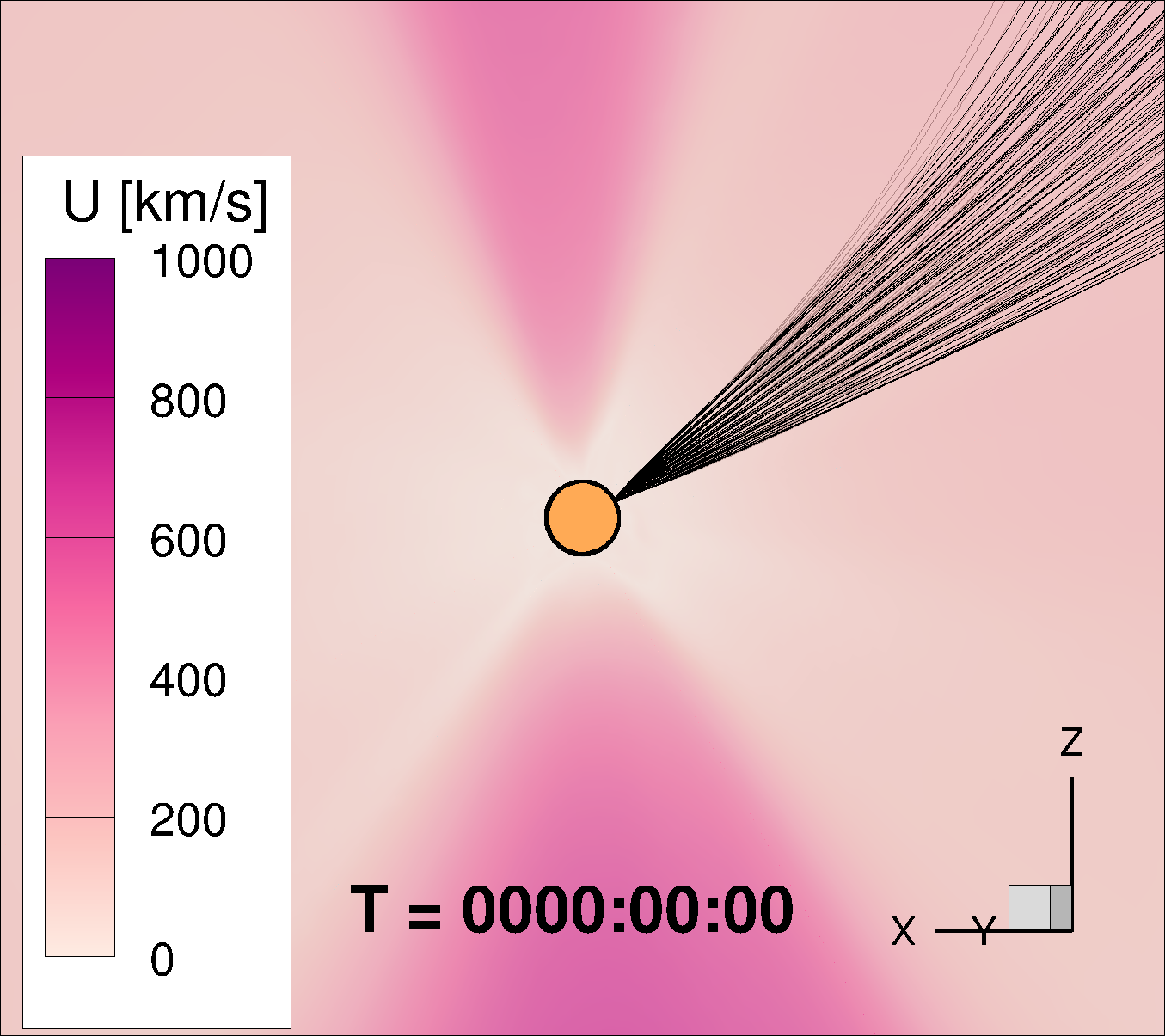
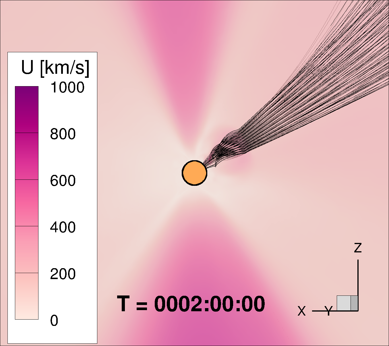
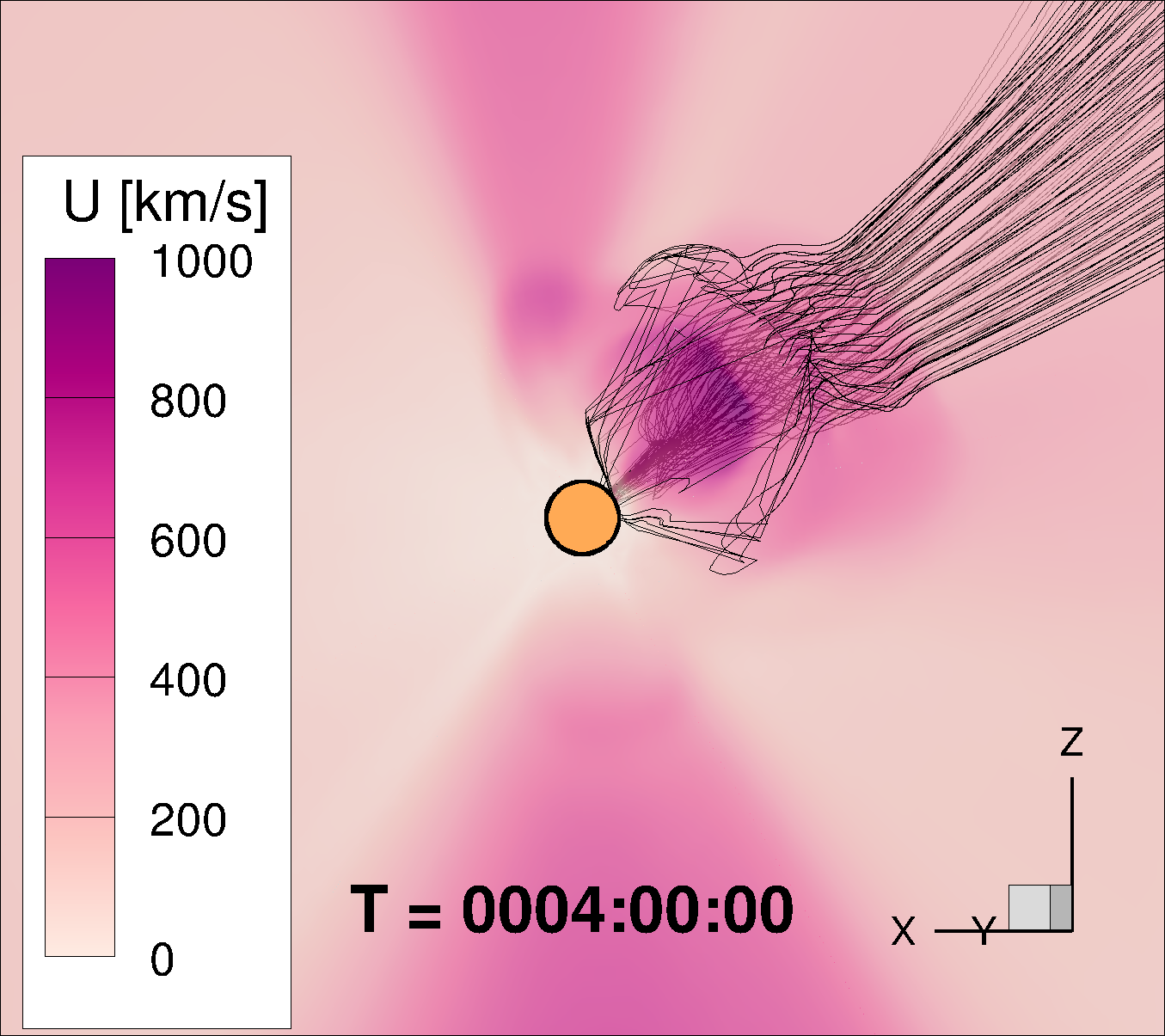
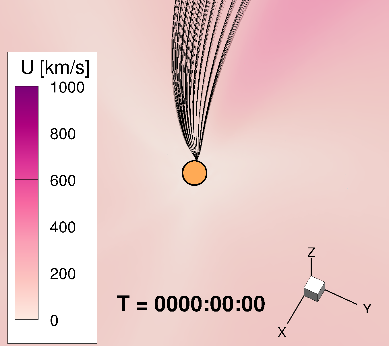
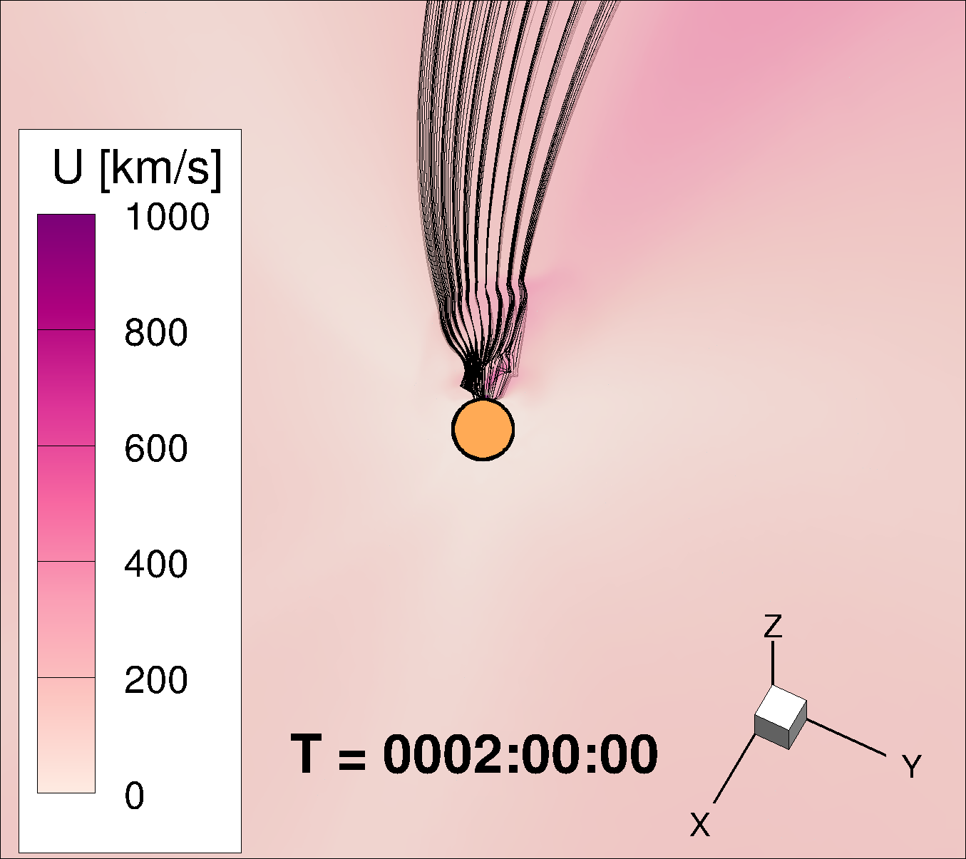
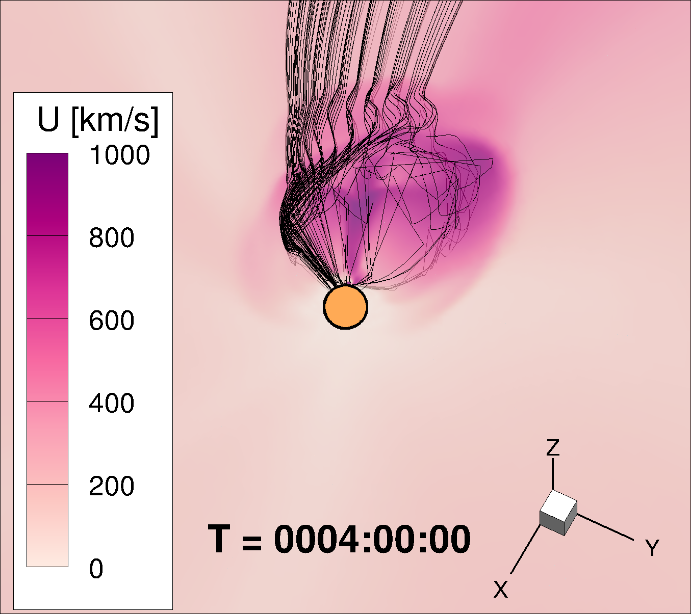
Figure 2: Three snapshots of a CME forming in the corona as seen from two angles in HGR: view onto plane of 29.5^∘ latitude (top) and plane of 208.5^∘ longitude (bottom). Color shows the speed of the solar wind. Thin black lines are magnetic field lines extracted from the MHD solution and imported to the kinetic code.

We present some results of the simulation below. Figure 2 shows three different snapshots (2 hours apart) of the CME forming in the solar corona together with extracted field lines. The CME was initiated at 29.5^∘ latitude and 208.5^∘ longitude in heliographic rotating coordinate system (HGR) and with anticipated speed $U_{\rm CME}=2000\,{\rm km/s}$. Figure 3 shows SEP flux for energies exceeding 10 MeV, which corresponds to NOAA GOES energy channel 2, along extracted field lines and through 1 AU sphere (interpolated between footprints of filed lines on that sphere). Finally, Figure 4 demonstrates a comparison of time evolution of SEP flux with GOES measurements.

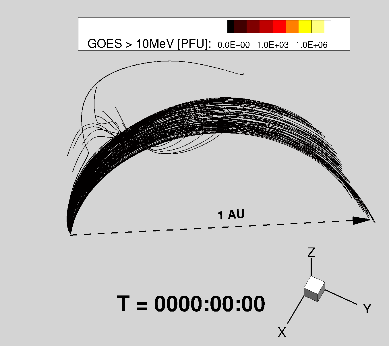
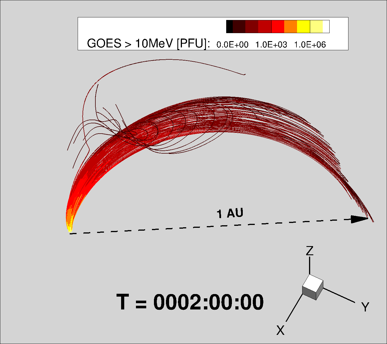
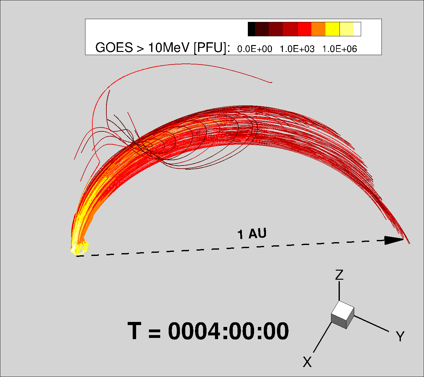
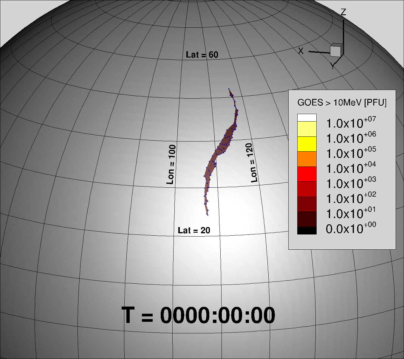
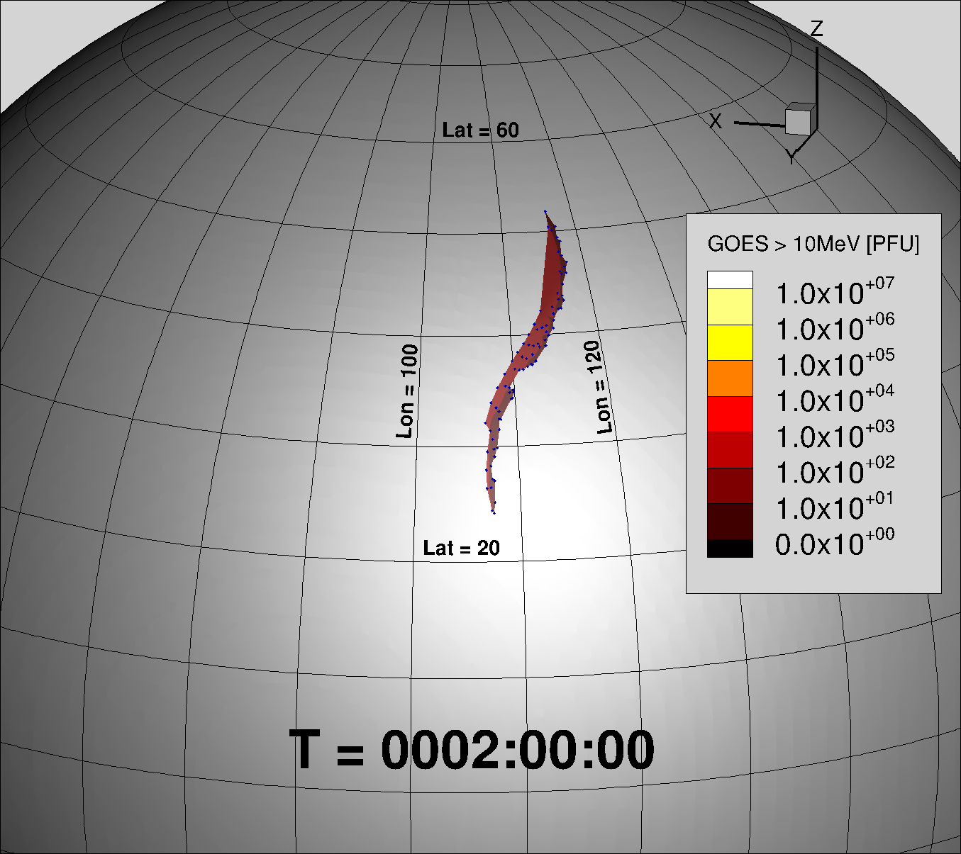
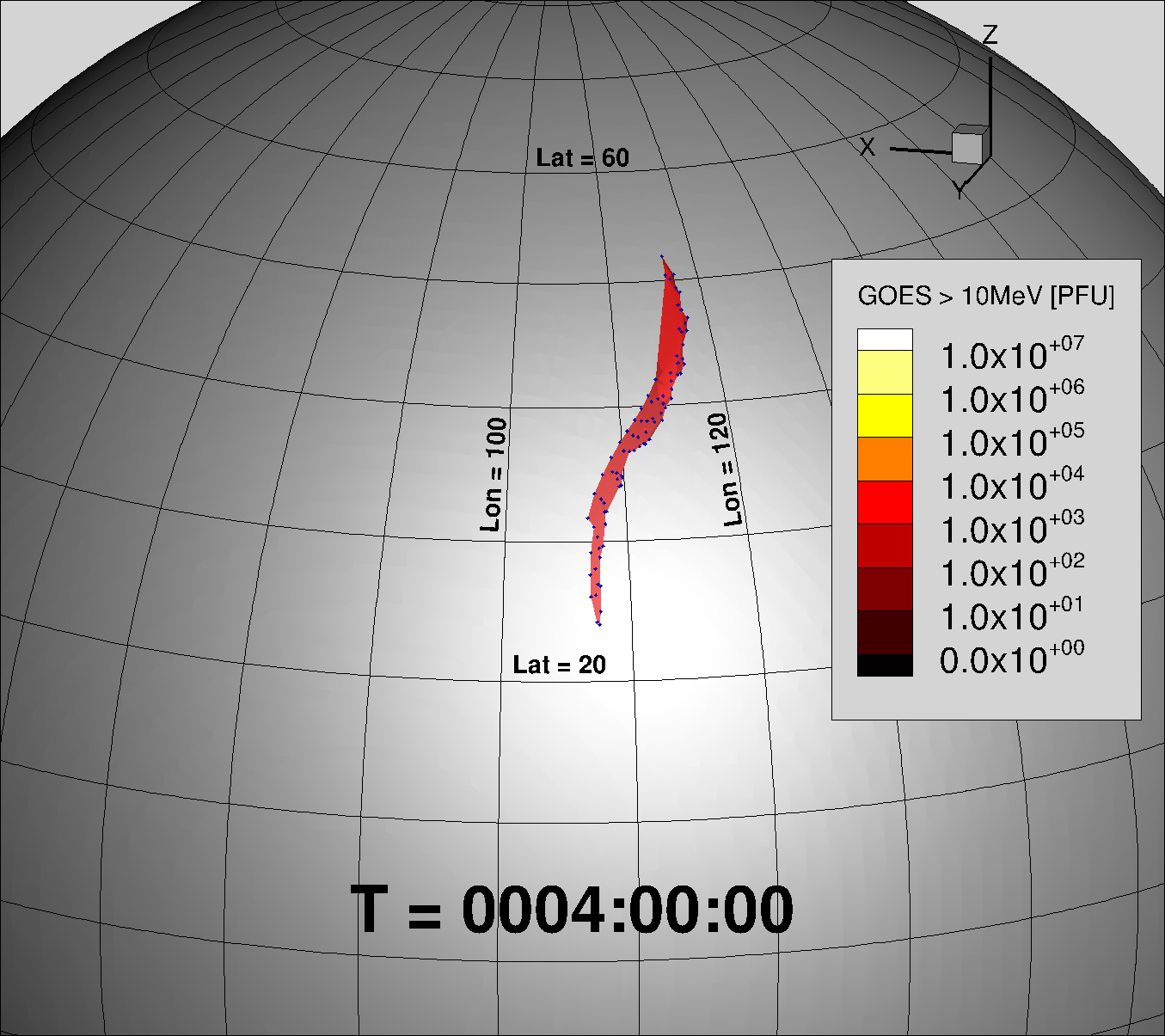
Figure 3: Simulated flux of SEP exceeding 10 MeV (GOES channel 2): along the extracted lines from the Sun to 1 AU (top) and interpolated between footprints (small blue diamonds) of lines on 1 AU sphere (bottom)

.

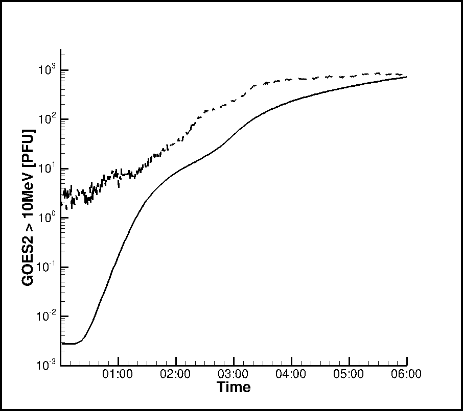
Figure 4: Time evolution of simulated flux of SEP exceeding 10 MeV (GOES channel 2) at 1 AU on a single line (solid black line) compared to GOES measurements (dashed black line). Time is measured from the CME initiation (4:00 on January 23, 2012).

6 Conclusions

The present paper serves the purpose of being a guide into and a reference for our research effort in the field of SEP forecasting. In this paper we have reviewed the physical principles that form the basis of the MHD component of our SEP forecasting framework. These principles serve as a foundation for a large number of computational models (developed over the span of several decades) that allow simulating quiet time SC and IH as well as eruptive events in SC and their propagation into IH. Here, however, we have put more focus on those models and tools (specifically, AWSoM, AWSoM-R, EEGGL) that have been or are being implemented in the Space Weather Modeling Framework (SWMF, Tóth et al., 2012), which is to host the full SEP forecasting framework. Additionally, we have suggested the concept of a magnetized cone model, that could serve as a simple, yet effective eruptive event generator.

The present paper is to be followed by the review of the kinetic component of our full SEP model and will complete its description.

7 Acknowledgements

The collaboration between the CCMC and University of Michigan is supported by the NSF SHINE grant 1257519(PI Aleksandre Taktakishvili). The work performed at the University of Michigan was partially supported by National Science Foundation grants AGS-1322543 and PHY-1513379, NASA grant NNX13AG25G, the European Union’s Horizon 2020 research and innovation program under grant agreement 637302PROGRESS. We would also like to acknowledge high-performance computing support from: (1) Yellowstone(ark:/85065/d7wd3xhc) provided by NCAR’s Computational and Information Systems Laboratory, sponsored by the National Science Foundation,and (2) Pleiades operated by NASA’s Advanced Supercomputing Division.

Appendix A Equilibrium Magnetic Configurations: Spheromak

The equations of MHD equilibrium read (Landau and Lifshitz, 1960):

$${\mathbf{j}}\times{\mathbf{B}}-{\nabla}P=0,$$ (A1)

which we consider in spherical coordinates $\left(r,\theta,\varphi\right)$. Herewith, $\mathbf{B}$ is the vector of magnetic field, $\mathbf{j}$ is the electric current and $P$ is the plasma pressure. It has been demonstrated (Grad and Rubin, 1958; Shafranov, 1966) that an axisymmetric equilibrium MHD configuration is governed by a single scalar equation, commonly referred to as the Grad-Shafranov equation. The key concept that allows transforming Eq. A1 to this simpler form is that of magnetic surfaces, which are defined as surfaces of constant pressure, $P$.

From Eq. A1, ${\mathbf{j}}\cdot{\nabla}P=0$ and ${\mathbf{B}}\cdot{\nabla}P=0$, i.e. a single line of either magnetic field, or electric current is entirely confined within a single magnetic surface. Further, magnetic field flux and current functions defined as

$${\psi}\left({r}_{\perp},{z}\right) = \int_{0}^{{r}_{\perp}}{{B}_{z}({r}_{\perp}^{\prime},{z}){r}_{\perp}^{\prime}d{r}_{\perp}^{\prime}}$$

$${I}\left({r}_{\perp},{z}\right) = \int_{0}^{{r}_{\perp}}{{j}_{z}({r}_{\perp}^{\prime},{z}){r}_{\perp}^{\prime}d{r}_{\perp}^{\prime}}$$ (A2)

can both be demonstrated to be constant on a given magnetic surface (herewith, ${r}_{\perp}={r}\sin\theta$ and ${z}={r}\cos\theta$). Therefore, for an axisymmetric equilibrium configuration, there is a functional dependence between ${\psi}$, ${I}$ and ${P}$: ${I}{=}{I}({\psi})$, $P{=}P({\psi})$. Using Ampere’s law, ${\nabla}\times\mathbf{{B}}=\mu_{0}\mathbf{j}$, and by introducing the toroidal component of the vector potential, $\nabla\times\mathbf{A}=\mathbf{{B}}$, one can relate the current and magnetic flux via the toroidal components of the field and vector potential: $I=\frac{{r}_{\perp}}{\mu_{0}}{B}_{\varphi}$, $\psi={r}_{\perp}A_{\varphi}$. Thus, the total magnetic field may be expressed as:

$$\mathbf{B}=\nabla\times\left(A_{\varphi}\mathbf{e}_{\varphi}\right)+B_{\varphi}\mathbf{e}_{\varphi}=\frac{1}{{r}_{\perp}}\left(\nabla\psi\times\mathbf{e}_{\varphi}+\mu_{0}I\mathbf{e}_{\varphi}\right)$$ (A3)

Herewith, ${\bf e}_{\varphi}$ is the unit vector of the azimuthal (toroidal) direction. Analogously, for the current density vector we have:

$$\mu_{0}\mathbf{j}=\nabla\times\left[\nabla\times\left(A_{\varphi}\mathbf{e}_{\varphi}\right)+{B}_{\varphi}\mathbf{e}_{\varphi}\right]=-\nabla^{2}\left(A_{\varphi}\mathbf{e}_{\varphi}\right)+\mu_{0}\frac{dI}{d\psi}\frac{\nabla\psi\times\mathbf{e}_{\varphi}}{{r}_{\perp}}$$ (A4)

Once substitutions Eq. A3 and Eq. A4 are performed and a common factor of $\frac{\nabla\psi}{{r}_{\perp}}$ is omitted, the condition of equilibrium, Eq. A1, reads

$$\mathbf{e}_{\varphi}\cdot\nabla^{2}(A_{\varphi}{\bf e}_{\varphi})=-\mu_{0}{r}_{\perp}\frac{dP}{d\psi}-\mu_{0}\frac{dI}{d\psi}B_{\varphi}.$$ (A5)

In the particular case of constant $\frac{dI}{d\psi}$ and $\frac{dP}{d\psi}$, by expressing the Laplace operator in spherical coordinates Eq. A5 reduces to the equation describing electro-magnetic waves (magnetic dipole and multipole harmonics - see Jackson, 1999):

$$\frac{1}{{r}^{2}}\frac{\partial}{\partial{r}}\left({r}^{2}\frac{\partial A_{\varphi}}{\partial{r}}\right)+\frac{1}{{r}^{2}\sin\theta}\frac{\partial}{\partial\theta}\left(\sin\theta\frac{\partial A_{\varphi}}{\partial\theta}\right)-\frac{A_{\varphi}}{{r}^{2}\sin^{2}\theta}+\alpha_{0}^{2}A_{\varphi}=-\mu_{0}{r}\sin\theta\frac{dP}{d\psi}$$ (A6)

where $\alpha_{0}=\mu_{0}dI/d\psi$. It may be solved by developing the solution over spherical harmonics: $A_{\varphi}=\sum_{n=1}^{\infty}{c_{n}j_{n}(\alpha_{0}{r})P^{1}_{n}(\cos\theta)}-\mu_{0}\alpha_{0}^{-2}{r}\sin\theta\frac{dP}{d\psi}$, where $P_{n}^{1}$ are associated Legendre polynomials, $j_{n}(x)=\sqrt{\frac{\pi}{2x}}J_{n+1/2}(x)$, $J_{\nu}(x)$ and $j_{n}(x)$ are regular and spherical Bessel functions respectively. For a dipole harmonic we have:

$$A_{\varphi}=A_{\varphi 0}\left[j_{1}(\alpha_{0}{r})-\frac{\mu_{0}{r}}{\alpha_{0}^{2}A_{\varphi 0}}\frac{dP}{d\psi}\right]\sin\theta$$ (A7)

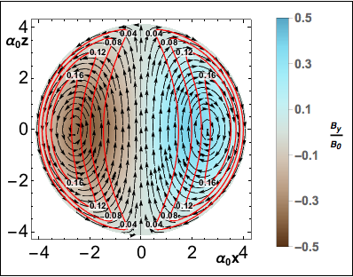
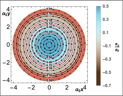
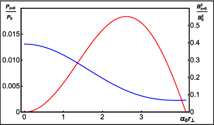
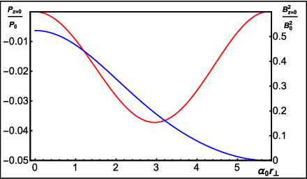
Figure 5: Top: spheromak configuration for $\beta_{0}{=}0.02$: meridional (left) and equatorial (right) planes. Magnetic field direction is marked with arrows, off-plane component of the magnetic field is normalized per $B_{0}$ (see Eq. 3.1) and shown by color. Local values of plasma parameter $\beta({\bf r})=\mu_{0}P({\bf r})/B^{2}({\bf r})$ are shown with orange curves corresponding to levels $\beta=0.04,0.08,0.12,0.16$ as marked explicitly. Bottom: radial dependence of thermal pressure, $\mu_{0}P(r)/B^{2}_{0}$, (red curve) and magnetic pressure, $B^{2}(r)/B^{2}_{0}$, (blue curve) in the equatorial cut ${z}{=}0$: for $\beta_{0}{=}0.02$ (left panel) and for $\beta_{0}{=}-2.87{\times}10^{-2}$ (right panel) .

Introducing parameters $B_{0}=\alpha_{0}A_{\varphi 0}$ and $\beta_{0}=\frac{\mu_{0}}{B_{0}\alpha_{0}^{2}}\frac{dP}{d\psi}$, we obtain the expression for th spheromak’s magnetic field and pressure:

$${\bf B}_{\rm sk}({\bf r})=\left[\frac{j_{1}({\alpha_{0}}{r})}{\alpha_{0}{r}}-\beta_{0}\right]\left(2{\bf B}_{0}+\sigma_{h}\alpha_{0}[{\bf B}_{0}\times{\bf r}]\right)+j_{2}(\alpha_{0}{r})\frac{[{\bf r}\times[{\bf r}\times{\bf B}_{0}]]}{r^{2}}$$ (A8)

$$P_{\rm sk}({\bf r})=\left[\frac{j_{1}({\alpha_{0}}{r})}{\alpha_{0}{r}}-\beta_{0}\right]\frac{\beta_{0}\alpha_{0}^{2}[{\bf r}\times{\bf B}_{0}]^{2}}{\mu_{0}}.$$ (A9)

Herewith, the vector ${\bf B}_{0}$ is introduced with the magnitude equal to $B_{0}$ directed along the polar axis of the spherical coordinate system, $\sigma_{h}=\pm 1$ is the sign of helicity (we assume $\alpha_{0}>0$). At the center of configuration the magnetic field equals ${\bf B}_{\rm sk}|_{r=0}=2\left(\frac{1}{3}-\beta_{0}\right){\bf B}_{0}$, which for low-beta plasma is only by a numerical factor of ${\approx}0.7$ differs from ${\bf B}_{0}$. In Eqs. A8-A9, the coordinate vector, ${\bf r}$, originates at the center of configuration, $\mathbf{R}_{\rm c}$. Thus, in the arbitrary coordinate system, the field and pressure of the configuration equal: ${\bf B}_{\rm sk}({\bf R}-{\bf R}_{\rm c})$, $p_{\rm sk}({\bf R}-{\bf R}_{\rm c})$, for $\|{\bf R}-{\bf R}_{\rm c}\|\leq r_{0}$.

We restrict currents to within a spherical magnetic surface $\|{\bf R}-{\bf R}_{\rm c}\|=r_{0}$. The radial and toroidal components of the magnetic field turn to zero at the surface, thus $j_{1}(\alpha_{0}r_{0})=\beta_{0}\alpha_{0}r_{0}$. For a given $\beta_{0}$ this equation relates the configuration size, $r_{0}$, with the extent of magnetic field twisting, $\alpha_{0}$, needed to close the configuration within this size. The plasma pressure, $P$, also turns to zero at the external boundary.

The meridional and equatorial planes (top) and radial dependence of the field and pressure for $\beta_{0}{=}0.02$ (bottom left) are shown in Fig. 5. The shown magnetic field lines are also the cross-sections of magnetic surfaces.

References

- Aguilar et al. (2015) Aguilar, M., D. Aisa, B. Alpat, A. Alvino, G. Ambrosi, K. Andeen, L. Arruda, N. Attig, P. Azzarello, A. Bachlechner, F. Barao, A. Barrau, L. Barrin, A. Bartoloni, L. Basara, M. Battarbee, R. Battiston, J. Bazo, U. Becker, M. Behlmann, B. Beischer, J. Berdugo, B. Bertucci, G. Bigongiari, V. Bindi, S. Bizzaglia, M. Bizzarri, G. Boella, W. de Boer, K. Bollweg, V. Bonnivard, B. Borgia, S. Borsini, M. J. Boschini, M. Bourquin, J. Burger, F. Cadoux, X. D. Cai, M. Capell, S. Caroff, J. Casaus, V. Cascioli, G. Castellini, I. Cernuda, D. Cerreta, F. Cervelli, M. J. Chae, Y. H. Chang, A. I. Chen, H. Chen, G. M. Cheng, H. S. Chen, L. Cheng, H. Y. Chou, E. Choumilov, V. Choutko, C. H. Chung, C. Clark, R. Clavero, G. Coignet, C. Consolandi, A. Contin, C. Corti, E. Cortina Gil, B. Coste, W. Creus, M. Crispoltoni, Z. Cui, Y. M. Dai, C. Delgado, S. Della Torre, M. B. Demirköz, L. Derome, S. Di Falco, L. Di Masso, F. Dimiccoli, C. Díaz, P. von Doetinchem, F. Donnini, W. J. Du, M. Duranti, D. D’Urso, A. Eline, F. J. Eppling, T. Eronen, Y. Y. Fan, L. Farnesini, J. Feng, E. Fiandrini, A. Fiasson, E. Finch, P. Fisher, Y. Galaktionov, G. Gallucci, B. García, R. García-López, C. Gargiulo, H. Gast, I. Gebauer, M. Gervasi, A. Ghelfi, W. Gillard, F. Giovacchini, P. Goglov, J. Gong, C. Goy, V. Grabski, D. Grandi, M. Graziani, C. Guandalini, I. Guerri, K. H. Guo, D. Haas, M. Habiby, S. Haino, K. C. Han, Z. H. He, M. Heil, J. Hoffman, T. H. Hsieh, Z. C. Huang, C. Huh, M. Incagli, M. Ionica, W. Y. Jang, H. Jinchi, K. Kanishev, G. N. Kim, K. S. Kim, Th. Kirn, R. Kossakowski, O. Kounina, A. Kounine, V. Koutsenko, M. S. Krafczyk, G. La Vacca, E. Laudi, G. Laurenti, I. Lazzizzera, A. Lebedev, H. T. Lee, S. C. Lee, C. Leluc, G. Levi, H. L. Li, J. Q. Li, Q. Li, Q. Li, T. X. Li, W. Li, Y. Li, Z. H. Li, Z. Y. Li, S. Lim, C. H. Lin, P. Lipari, T. Lippert, D. Liu, H. Liu, M. Lolli, T. Lomtadze, M. J. Lu, S. Q. Lu, Y. S. Lu, K. Luebelsmeyer, J. Z. Luo, S. S. Lv, R. Majka, C. Mañá, J. Marín, T. Martin, G. Martínez, N. Masi, D. Maurin, A. Menchaca-Rocha, Q. Meng, D. C. Mo, L. Morescalchi, P. Mott, M. Müller, J. Q. Ni, N. Nikonov, F. Nozzoli, P. Nunes, A. Obermeier, A. Oliva, M. Orcinha, F. Palmonari, C. Palomares, M. Paniccia, A. Papi, M. Pauluzzi, E. Pedreschi, S. Pensotti, R. Pereira, N. Picot-Clemente, F. Pilo, A. Piluso, C. Pizzolotto, V. Plyaskin, M. Pohl, V. Poireau, E. Postaci, A. Putze, L. Quadrani, X. M. Qi, X. Qin, Z. Y. Qu, T. Räihä, P. G. Rancoita, D. Rapin, J. S. Ricol, I. Rodríguez, S. Rosier-Lees, A. Rozhkov, D. Rozza, R. Sagdeev, J. Sandweiss, P. Saouter, C. Sbarra, S. Schael, S. M. Schmidt, A. Schulz von Dratzig, G. Schwering, G. Scolieri, E. S. Seo, B. S. Shan, Y. H. Shan, J. Y. Shi, X. Y. Shi, Y. M. Shi, T. Siedenburg, D. Son, F. Spada, F. Spinella, W. Sun, W. H. Sun, M. Tacconi, C. P. Tang, X. W. Tang, Z. C. Tang, L. Tao, D. Tescaro, Samuel C. C. Ting, S. M. Ting, N. Tomassetti, J. Torsti, C. Türkoğlu, T. Urban, V. Vagelli, E. Valente, C. Vannini, E. Valtonen, S. Vaurynovich, M. Vecchi, M. Velasco, J. P. Vialle, V. Vitale, S. Vitillo, L. Q. Wang, N. H. Wang, Q. L. Wang, R. S. Wang, X. Wang, Z. X. Wang, Z. L. Weng, K. Whitman, J. Wienkenhöver, H. Wu, X. Wu, X. Xia, M. Xie, S. Xie, R. Q. Xiong, G. M. Xin, N. S. Xu, W. Xu, Q. Yan, J. Yang, M. Yang, Q. H. Ye, H. Yi, Y. J. Yu, Z. Q. Yu, S. Zeissler, J. H. Zhang, M. T. Zhang, X. B. Zhang, Z. Zhang, Z. M. Zheng, H. L. Zhuang, V. Zhukov, A. Zichichi, N. Zimmermann, P. Zuccon, and C. Zurbach, Precision measurement of the proton flux in primary cosmic rays from rigidity 1 gv to 1.8 tv with the alpha magnetic spectrometer on the international space station, Phys. Rev. Lett., 114, 171103, Apr 2015.
- Alazraki and Couturier (1971) Alazraki, G., and P. Couturier, Solar Wind Acceleration Caused by the Gradient of Alfvén Wave Pressure, Astron. & Astrophys., 13, 380, August 1971.
- Alfvén (1942) Alfvén, H., Existence of Electromagnetic-Hydrodynamic Waves, Nature, 150, 405–406, October 1942.
- Antiochos et al. (1999) Antiochos, S. K., C. R. DeVore, and J. A. Klimchuk, A Model for Solar Coronal Mass Ejections, ApJ, 510, 485–493, January 1999.
- Arge and Pizzo (2000) Arge, C. N., and V. J. Pizzo, Improvement in the prediction of solar wind conditions using near-real time solar magnetic field updates, J. Geophys. Res., 105, 10465–10480, May 2000.
- Arge et al. (2003) Arge, C. N., D. Odstrcil, V. J. Pizzo, and L. R. Mayer, Improved Method for Specifying Solar Wind Speed Near the Sun, In Velli, M., R. Bruno, F. Malara, and B. Bucci, editors, Solar Wind Ten, volume 679 of American Institute of Physics Conference Series, pages 190–193, September 2003.
- Axford et al. (1977) Axford, W. I., E. Leer, and G. Skadron, The acceleration of cosmic rays by shock waves, International Cosmic Ray Conference, 11, 132–137, 1977.
- Barnes (1966) Barnes, A., Collisionless Damping of Hydromagnetic Waves, Physics of Fluids, 9, 1483–1495, August 1966.
- Barnes (1968) Barnes, A., Collisionless Heating of the Solar-Wind Plasma. I. Theory of the Heating of Collisionless Plasma by Hydromagnetic Waves, ApJ, 154, 751, November 1968.
- Belcher and Davis (1971) Belcher, J. W., and L. Davis, Jr., Large-amplitude Alfvén waves in the interplanetary medium, 2, J. Geophys. Res., 76, 3534, 1971.
- Belcher et al. (1969) Belcher, J. W., L. Davis, Jr., and E. J. Smith, Large-amplitude Alfvén waves in the interplanetary medium: Mariner 5, J. Geophys. Res., 74, 2302, 1969.
- Bell (1978a) Bell, A. R., The acceleration of cosmic rays in shock fronts. I, MNRAS, 182, 147–156, January 1978a.
- Bell (1978b) Bell, A. R., The acceleration of cosmic rays in shock fronts. II, MNRAS, 182, 443–455, February 1978b.
- Blandford and Ostriker (1978) Blandford, R. D., and J. P. Ostriker, Particle acceleration by astrophysical shocks, ApJ, 221, L29–L32, April 1978.
- Borovikov et al. (2015) Borovikov, Dmitry, Igor V. Sokolov, and Gábor Tóth, An efficient second-order accurate and continuous interpolation for block-adaptive grids, J. Comput. Physics, 297, 599–610, 2015.
- Borovikov et al. (2017) Borovikov, D., I. V. Sokolov, W. B. Manchester, M. Jin, and T. I. Gombosi, Eruptive event generator based on the Gibson-Low magnetic configuration, Journal of Geophysical Research (Space Physics), 122, 7979–7984, August 2017.
- Brueckner et al. (1995) Brueckner, G. E., R. A. Howard, M. J. Koomen, C. M. Korendyke, D. J. Michels, J. D. Moses, D. G. Socker, K. P. Dere, P. L. Lamy, A. Llebaria, M. V. Bout, R. Schwenn, G. M. Simnett, D. K. Bedford, and C. J. Eyles, The Large Angle Spectroscopic Coronagraph (LASCO), Sol. Phys., 162, 357–402, December 1995.
- Cane et al. (2006) Cane, H. V., R. A. Mewaldt, C. M. S. Cohen, and T. T. von Rosenvinge, Role of flares and shocks in determining solar energetic particle abundances, Journal of Geophysical Research (Space Physics), 111, A06S90, June 2006.
- Cliver et al. (2004) Cliver, E. W., S. W. Kahler, and D. V. Reames, Coronal Shocks and Solar Energetic Proton Events, ApJ, 605, 902–910, April 2004.
- Cliver (2006) Cliver, E. W., The 1859 space weather event: Then and now, Adv. Space Res., 38( 2 ), 119–129, 2006.
- Cliver (2009) Cliver, E. W., History of research on solar energetic particle (SEP) events: the evolving paradigm, In Gopalswamy, N., and D. F. Webb, editors, Universal Heliophysical Processes, volume 257 of IAU Symposium, pages 401–412, March 2009.
- Cohen et al. (1999) Cohen, C. M. S., R. A. Mewaldt, R. A. Leske, A. C. Cummings, E. C. Stone, M. E. Wiedenbeck, E. R. Christian, and T. T. von Rosenvinge, New observations of heavy-ion-rich solar particle events from ACE, Geophys. Res. Lett., 26, 2697–2700, 1999.
- Cohen et al. (2007) Cohen, O., I. V. Sokolov, I. I. Roussev, C. N. Arge, W. B. Manchester, T. I. Gombosi, R. A. Frazin, H. Park, M. D. Butala, F. Kamalabadi, and M. Velli, A semiempirical magnetohydrodynamical model of the solar wind, Astrophys. J. Lett., 654, L163–L166, January 2007.
- Cohen et al. (2008) Cohen, O., I. V. Sokolov, I. I. Roussev, and T. I. Gombosi, Validation of a synoptic solar wind model, J. Geophys. Res., 113( A12 ), A03104, March 2008.
- Coleman (1966) Coleman, P. J., Jr., Variations in the interplanetary magnetic field: Mariner 2: 1. Observed properties, J. Geophys. Res., 71, 5509–5531, December 1966.
- Coleman (1967) Coleman, P. J., Jr., Wave-like phenomena in the interplanetary plasma: Mariner 2, Planet. Space Sci., 15, 953–973, June 1967.
- Coleman (1968) Coleman, P. J., Jr., Turbulence, Viscosity, and Dissipation in the Solar-Wind Plasma, ApJ, 153, 371, August 1968.
- Cranmer (2010) Cranmer, S. R., An Efficient Approximation of the Coronal Heating Rate for use in Global Sun-Heliosphere Simulations, ApJ, 710, 676–688, February 2010.
- Dewar (1970) Dewar, R. L., Interaction between Hydromagnetic Waves and a Time-Dependent, Inhomogeneous Medium, Physics of Fluids, 13, 2710–2720, November 1970.
- Dmitruk et al. (2002) Dmitruk, P., W. H. Matthaeus, L. J. Milano, S. Oughton, G. P. Zank, and D. J. Mullan, Coronal Heating Distribution Due to Low-Frequency, Wave-driven Turbulence, ApJ, 575, 571–577, August 2002.
- Downs et al. (2010) Downs, C., I. I. Roussev, B. van der Holst, N. Lugaz, I. V. Sokolov, and T. I. Gombosi, Toward a Realistic Thermodynamic Magnetohydrodynamic Model of the Global Solar Corona, ApJ, 712, 1219–1231, April 2010.
- Elsässer (1950) Elsässer, W. M., The Hydromagnetic Equations, Physical Review, 79, 183–183, July 1950.
- Fan and Gibson (2004) Fan, Y., and S. E. Gibson, Numerical simulations of three-dimensional coronal magnetic fields resulting from the emergence of twisted magnetic flux tubes, The Astrophysical Journal, 609( 2 ), 1123, 2004.
- Fermi (1949) Fermi, E., On the origin of the cosmic radiation, Phys. Rev., 75, 1169–1174, Apr 1949.
- Forbush (1946) Forbush, S. E., Three Unusual Cosmic-Ray Increases Possibly Due to Charged Particles from the Sun, Physical Review, 70, 771–772, November 1946.
- Gibson and Low (1998) Gibson, S. E., and B. C. Low, A Time-Dependent Three-Dimensional Magnetohydrodynamic Model of the Coronal Mass Ejection, Astrophys. J., 493, 460–473, January 1998.
- Gopalswamy et al. (2001) Gopalswamy, N., A. Lara, M. L. Kaiser, and J.-L. Bougeret, Near-Sun and near-Earth manifestations of solar eruptions, J. Geophys. Res., 106, 25261–25278, November 2001.
- Gopalswamy et al. (2012) Gopalswamy, N., H. Xie, S. Yashiro, S. Akiyama, P. Mäkelä, and I. G. Usoskin, Properties of Ground Level Enhancement Events and the Associated Solar Eruptions During Solar Cycle 23, Space Sci. Rev., 171, 23–60, October 2012.
- Gopalswamy et al. (2014) Gopalswamy, N., H. Xie, S. Akiyama, P. A. Mäkelä, and S. Yashiro, Major solar eruptions and high-energy particle events during solar cycle 24, Earth, Planets, and Space, 66, 104, December 2014.
- Gosling (1993) Gosling, J. T., The solar flare myth, J. Geophys. Res., 98, 18937–18950, November 1993.
- Grad and Rubin (1958) Grad, H., and H Rubin, Hydromagnetic Equilibria and Force-Free Fields, In Proceedings of the 2nd UN Conference on the Peaceful Uses of Atomic Energy, volume 31, pages 190–197, 1958.
- Grechnev et al. (2008) Grechnev, V. V., V. G. Kurt, I. M. Chertok, A. M. Uralov, H. Nakajima, A. T. Altyntsev, A. V. Belov, B. Y. Yushkov, S. N. Kuznetsov, L. K. Kashapova, N. S. Meshalkina, and N. P. Prestage, An Extreme Solar Event of 20 January 2005: Properties of the Flare and the Origin of Energetic Particles, Sol. Phys., 252, 149–177, October 2008.
- Green and Boardsen (2006) Green, J. L., and S. Boardsen, Duration and extent of the great auroral storm of 1859, Adv. Space Res., 38( 2 ), 130–135, 2006.
- Green et al. (2006) Green, James L., Scott Boardsen, Sten Odenwald, John Humble, and Katherine A. Pazamickas, Eyewitness reports of the great auroral storm of 1859, Adv. Space Res., 38( 2 ), 145–154, 2006.
- Gressl et al. (2014) Gressl, C., A. M. Veronig, M. Temmer, D. Odstrčil, J. A. Linker, Z. Mikić, and P. Riley, Comparative Study of MHD Modeling of the Background Solar Wind, Sol. Phys., 289, 1783–1801, May 2014.
- Heath et al. (1977) Heath, D. F., A. J. Krueger, and P. J. Crutzen, Solar proton event: influence on stratospheric ozone, Science, 197( 4306 ), 886–9, 1977.
- Heinemann and Olbert (1980) Heinemann, M., and S. Olbert, Non-WKB Alfven waves in the solar wind, J. Geophys. Res., 85, 1311–1327, March 1980.
- Hellweg and Baumstark-Khan (2007) Hellweg, C. E., and C. Baumstark-Khan, Getting ready for the manned mission to Mars: The astronauts’ risk from space radiation, Naturwissenschaften, 94( 7 ), 517–526, jan 2007.
- Hollweg (1986) Hollweg, J. V., Transition region, corona, and solar wind in coronal holes, J. Geophys. Res., 91, 4111–4125, April 1986.
- Hu et al. (2003) Hu, Y. Q., S. R. Habbal, Y. Chen, and X. Li, Are coronal holes the only source of fast solar wind at solar minimum?, Journal of Geophysical Research (Space Physics), 108, 1377, October 2003.
- Jackson (1999) Jackson, John David, Classical electrodynamics, Wiley, New York, NY, 3rd ed. edition, 1999.
- Jacques (1977) Jacques, S. A., Momentum and energy transport by waves in the solar atmosphere and solar wind, ApJ, 215, 942–951, August 1977.
- Jacques (1978) Jacques, S. A., Solar wind models with Alfven waves, ApJ, 226, 632–649, December 1978.
- Jäkel (2004) Jäkel, O., Radiation hazard during a manned mission to Mars, Zeitschrift fur medizinische Physik, 14( 4 ), 267–272, 2004.
- Jian et al. (2015) Jian, L. K., P. J. MacNeice, A. Taktakishvili, D. Odstrcil, B. Jackson, H.-S. Yu, P. Riley, I. V. Sokolov, and R. M. Evans, Validation for solar wind prediction at Earth: Comparison of coronal and heliospheric models installed at the CCMC, Space Weather, 13, 316–338, May 2015.
- Jin et al. (2013) Jin, M., W. B. Manchester, B. van der Holst, R. Oran, I. Sokolov, G. Toth, Y. Liu, X. D. Sun, and T. I. Gombosi, Numerical Simulations of Coronal Mass Ejection on 2011 March 7: One-temperature and Two-temperature Model Comparison, ApJ, 773, 50, August 2013.
- Jin et al. (2017a) Jin, M., W. B. Manchester, B. van der Holst, I. Sokolov, G. Tóth, R. E. Mullinix, A. Taktakishvili, A. Chulaki, and T. I. Gombosi, Data-constrained coronal mass ejections in a global magnetohydrodynamics model, The Astrophysical Journal, 834( 2 ), 173, 2017a.
- Jin et al. (2017b) Jin, M., W. B. Manchester, B. van der Holst, I. Sokolov, G. Tóth, A. Vourlidas, C. A. de Koning, and T. I. Gombosi, Chromosphere to 1 au simulation of the 2011 march 7th event: A comprehensive study of coronal mass ejection propagation, The Astrophysical Journal, 834( 2 ), 172, 2017b.
- Joshi et al. (2013) Joshi, N. C., W. Uddin, A. K. Srivastava, R. Chandra, N. Gopalswamy, P. K. Manoharan, M. J. Aschwanden, D. P. Choudhary, R. Jain, N. V. Nitta, H. Xie, S. Yashiro, S. Akiyama, P. Mäkelä, P. Kayshap, A. K. Awasthi, V. C. Dwivedi, and K. Mahalakshmi, A multiwavelength study of eruptive events on January 23, 2012 associated with a major solar energetic particle event, Advances in Space Research, 52, 1–14, July 2013.
- Joyce et al. (2015) Joyce, C. J., N. A. Schwadron, L. W. Townsend, R. A. Mewaldt, C. M. S. Cohen, T. T. Rosenvinge, A. W. Case, H. E. Spence, J. K. Wilson, M. Gorby, M. Quinn, and C. J. Zeitlin, Analysis of the potential radiation hazard of the 23 July 2012 SEP event observed by STEREO A using the EMMREM model and LRO/CRaTER, Space Weather, 13, 560–567, September 2015.
- Kahler et al. (1978) Kahler, S. W., E. Hildner, and M. A. I. Van Hollebeke, Prompt solar proton events and coronal mass ejections, Sol. Phys., 57, 429–443, April 1978.
- Kahler et al. (2012) Kahler, S. W., E. W. Cliver, A. J. Tylka, and W. F. Dietrich, A Comparison of Ground Level Event e/p and Fe/O Ratios with Associated Solar Flare and CME Characteristics, Space Sci. Rev., 171, 121–139, October 2012.
- Kahler (1994) Kahler, S., Injection profiles of solar energetic particles as functions of coronal mass ejection heights, ApJ, 428, 837–842, June 1994.
- Kóta et al. (2005) Kóta, J., W. B. Manchester, J. R. Jokipii, D. L. de Zeeuw, and T. I. Gombosi, Simulation of SEP Acceleration and Transport at CME-driven Shocks, In Li, G., G. P. Zank, and C. T. Russell, editors, The Physics of Collisionless Shocks: 4th Annual IGPP International Astrophysics Conference, volume 781 of American Institute of Physics Conference Series, pages 201–206, August 2005.
- Krymsky (1977) Krymsky, G. F., A regular mechanism for the acceleration of charged particles on the front of a shock wave, Akademiia Nauk SSSR Doklady, 234, 1306–1308, June 1977.
- Landau and Lifshitz (1960) Landau, L. D., and E. M. Lifshitz, Electrodynamics of continuous media, Pergamon Press: Oxford, 1960.
- Landi et al. (2013) Landi, E., P. R. Young, K. P. Dere, G. Del Zanna, and H. E. Mason, CHIANTI - An Atomic Database for Emission Lines. XIII. Soft X-Ray Improvements and Other Changes, ApJ, 763, 86, February 2013.
- Lee (1997) Lee, M. A., Particle Acceleration and Transport at CME-Driven Shocks, in Coronal Mass Ejections (eds N. Crooker, J. A. Joselyn and J. Feynman), Washington DC American Geophysical Union Geophysical Monograph Series, 99, 227–234, 1997.
- Leroy (1980) Leroy, B., Propagation of waves in an atmosphere in the presence of a magnetic field. II - The reflection of Alfven waves, A&A, 91, 136–146, November 1980.
- Li et al. (2003) Li, G., G. P. Zank, and W. K. M. Rice, Energetic Particle Acceleration and Transport at Coronal Mass Ejection-Driven Shocks, J. Geophys. Res., 108(A2), 10–21, February 2003.
- Linker et al. (2016) Linker, J., T. Torok, C. Downs, R. Lionello, V. Titov, R. M. Caplan, Z. Mikić, and P. Riley, MHD simulation of the Bastille day event, In American Institute of Physics Conference Series, volume 1720 of American Institute of Physics Conference Series, page 020002, March 2016.
- Lionello et al. (2001) Lionello, R., J. A. Linker, and Z. Mikić, Including the Transition Region in Models of the Large-Scale Solar Corona, ApJ, 546, 542–551, January 2001.
- Lionello et al. (2009) Lionello, R., J. A. Linker, and Z. Mikić, Multispectral Emission of the Sun During the First Whole Sun Month: Magnetohydrodynamic Simulations, ApJ, 690, 902–912, January 2009.
- Lionello et al. (2014a) Lionello, R., M. Velli, C. Downs, J. A. Linker, and Z. Mikić, Application of a Solar Wind Model Driven by Turbulence Dissipation to a 2D Magnetic Field Configuration, ApJ, 796, 111, December 2014a.
- Lionello et al. (2014b) Lionello, R., M. Velli, C. Downs, J. A. Linker, Z. Mikić, and A. Verdini, Validating a Time-dependent Turbulence-driven Model of the Solar Wind, ApJ, 784, 120, April 2014b.
- Low (1982) Low, B. C., Self-similar magnetohydrodynamics. I - The gamma = 4/3 polytrope and the coronal transient, ApJ, 254, 796–805, March 1982.
- Lugaz et al. (2005) Lugaz, N., W. B. Manchester, IV, and T. I. Gombosi, Numerical simulation of the interaction of two coronal mass ejections from sun to earth, ApJ, 634, 651–662, November 2005.
- Lugaz et al. (2007) Lugaz, N., W. B. Manchester, IV, I. I. Roussev, G. Tóth, and T. I. Gombosi, Numerical Investigation of the Homologous Coronal Mass Ejection Events from Active Region 9236, ApJ, 659, 788–800, April 2007.
- MacNeice (2009) MacNeice, P., Validation of community models: 2. Development of a baseline using the Wang-Sheeley-Arge model, Space Weather, 7, S12002, December 2009.
- Makhmutov et al. (2009) Makhmutov, V.S., G.A. Bazilevskaya, Y.I. Stozhkov, N.S. Svirzhevsky, and A.K. Svirzhevskaya, Ionisation state of the Earth’s stratosphere during powerful solar proton events, In Proc. 31st International Cosmic Ray Conference, Łódź, Poland, 2009.
- Manchester et al. (2004a) Manchester, W. B., T. I. Gombosi, I. Roussev, D. L. De Zeeuw, I. V. Sokolov, K. G. Powell, G. Tóth, and M. Opher, Three-dimensional MHD simulation of a flux rope driven CME, J. Geophys. Res., 109(A18), 1,102–1,119, January 2004a.
- Manchester et al. (2004b) Manchester, W. B., T. I. Gombosi, I. Roussev, A. Ridley, D. L. De Zeeuw, I. V. Sokolov, K. G. Powell, and G. Tóth, Modeling a space weather event from the Sun to the Earth: CME generation and interplanetary propagation, J. Geophys. Res., 109(A18), 2,107–2,122, February 2004b.
- Manchester et al. (2005) Manchester, W. B., T. I. Gombosi, D. L. De Zeeuw, I. V. Sokolov, I. I. Roussev, K. G. Powell, J. Kóta, G. Tóth, and T. H. Zurbuchen, Coronal mass ejection shock and sheath structures relevant to particle acceleration, AStrophys. J., 622, 1225–1239, 2005.
- Manchester et al. (2006) Manchester, W. B., A. J. Ridley, T. I. Gombosi, and D. L. DeZeeuw, Modeling the Sun-to-Earth propagation of a very fast CME, Advances in Space Research, 38, 253–262, January 2006.
- Manchester et al. (2008) Manchester, W. B., IV, A. Vourlidas, G. Tóth, N. Lugaz, I. I. Roussev, I. V. Sokolov, T. I. Gombosi, D. L. De Zeeuw, and M. Opher, Three-dimensional MHD Simulation of the 2003 October 28 Coronal Mass Ejection: Comparison with LASCO Coronagraph Observations, ApJ, 684, 1448–1460, September 2008.
- Manchester et al. (2012) Manchester, W. B., IV, B. van der Holst, G. Tóth, and T. I. Gombosi, The Coupled Evolution of Electrons and Ions in Coronal Mass Ejection-driven shocks, ApJ, 756, 81, September 2012.
- Matsumoto and Suzuki (2012) Matsumoto, T., and T. K. Suzuki, Connecting the Sun and the Solar Wind: The First 2.5-dimensional Self-consistent MHD Simulation under the Alfvén Wave Scenario, ApJ, 749, 8, April 2012.
- Matthaeus et al. (1999) Matthaeus, W. H., G. P. Zank, S. Oughton, D. J. Mullan, and P. Dmitruk, Coronal Heating by Magnetohydrodynamic Turbulence Driven by Reflected Low-Frequency Waves, ApJ, 523, L93–L96, September 1999.
- Matthiä et al. (2009) Matthiä, D., B. Heber, G. Reitz, M. Meier, L. Sihver, T. Berger, and K. Herbst, Temporal and spatial evolution of the solar energetic particle event on 20 January 2005 and resulting radiation doses in aviation, Journal of Geophysical Research (Space Physics), 114, A08104, August 2009.
- Mays et al. (2015) Mays, M. L., A. Taktakishvili, A. Pulkkinen, P. J. MacNeice, L. Rastätter, D. Odstrcil, L. K. Jian, I. G. Richardson, J. A. LaSota, Y. Zheng, and M. M. Kuznetsova, Ensemble Modeling of CMEs Using the WSA-ENLIL+Cone Model, Sol. Phys., 290, 1775–1814, June 2015.
- Mazur et al. (1999) Mazur, J. E., G. M. Mason, M. D. Looper, R. A. Leske, and R. A. Mewaldt, Charge states of solar energetic particles using the geomagnetic cutoff technique: SAMPEX measurements in the 6 November 1997 solar particle event, Geophys. Res. Lett., 26, 173–176, 1999.
- Meyer et al. (1956) Meyer, P., E. N. Parker, and J. A. Simpson, Solar Cosmic Rays of February, 1956 and Their Propagation through Interplanetary Space, Physical Review, 104, 768–783, November 1956.
- Michalek (2006) Michalek, G., An Asymmetric Cone Model for Halo Coronal Mass Ejections, Sol. Phys., 237, 101–118, August 2006.
- Mikić et al. (2007) Mikić, Z., J.A. Linker, R. Lionello, P. Riley, and V. Titov, Predicting the structure of the solar corona for the total solar eclipse of march 29, 2006, Solar and stellar physics through eclipses, ASP Conf. Ser., 370, 299–307, 2007.
- Morris (2007) Morris, Doug, From the Flight Deck: Plane Talk and Sky Science, ECW Press, Toronto, Ontario, Canada, 2007.
- Nesse Tyssøy et al. (2013) Nesse Tyssøy, H., J. Stadsnes, F. SøRaas, and M. SøRbø, Variations in cutoff latitude during the January 2012 solar proton event and implication for the distribution of particle energy deposition, Geophys. Res. Lett., 40, 4149–4153, August 2013.
- Ng et al. (1999) Ng, C. K., D. V. Reames, and A. J. Tylka, Effect of proton-amplified waves on the evolution of solar energetic particle composition in gradual events, Geophys. Res. Lett., 26, 2145–2148, 1999.
- Ng et al. (2003) Ng, C. K., D. V. Reames, and A. J. Tylka, Modeling Shock-accelerated Solar Energetic Particles Coupled to Interplanetary Alfvén Waves, ApJ, 591, 461–485, July 2003.
- Norquist and Meeks (2010) Norquist, D. C., and W. C. Meeks, A comparative verification of forecasts from two operational solar wind models, Space Weather, 8, S12005, December 2010.
- Oran et al. (2013) Oran, R., B. van der Holst, E. Landi, M. Jin, I. V. Sokolov, and T. I. Gombosi, A Global Wave-driven Magnetohydrodynamic Solar Model with a Unified Treatment of Open and Closed Magnetic Field Topologies, ApJ, 778, 176, December 2013.
- Owens et al. (2008) Owens, M. J., H. E. Spence, S. McGregor, W.J. Hughes, J. M. Quinn, C. N. Arge, P. Riley, J. Linker, and D. Odstrčil, Metrics for solar wind prediction models: Comparison of empirical, hybrid and physics-based schemes with 8-years of l1 observations, Space Weather, 6, 2008.
- Parker (1965) Parker, E. N., The passage of energetic charged particles through interplanetary space, Planet. Space Sci., 13, 9–49, January 1965.
- Plunkett et al. (1998) Plunkett, S. P., B. J. Thompson, R. A. Howard, D. J. Michels, O. C. St. Cyr, S. J. Tappin, R. Schwenn, and P. L. Lamy, LASCO observations of an Earth-directed coronal mass ejection on May 12, 1997, Geophys. Res. Lett., 25, 2477–2480, 1998.
- Reames (1999) Reames, D. V., Particle Acceleration at the Sun and in the Heliosphere, Space Sci. Rev., 90, 413–491, February 1999.
- Reames (2002) Reames, D. V., Magnetic Topology of Impulsive and Gradual Solar Energetic Particle Events, ApJ, 571, L63–L66, May 2002.
- Reiss et al. (2016) Reiss, M. A., M. Temmer, A. M. Veronig, L. Nikolic, S. Vennerstrom, F. Schöngassner, and S. J. Hofmeister, Verification of high-speed solar wind stream forecasts using operational solar wind models, Space Weather, 14, 495–510, July 2016.
- Rice et al. (2003) Rice, W. K. M., G. P. Zank, and G. Li, Particle acceleration and coronal mass ejection driven shocks: Shocks of arbitrary strength, Journal of Geophysical Research (Space Physics), 108, 1369, October 2003.
- Riley et al. (2006) Riley, P., J. A. Linker, Z. Mikić, R. Lionello, S. A. Ledvina, and J. G. Luhmann, A Comparison between Global Solar Magnetohydrodynamic and Potential Field Source Surface Model Results, ApJ, 653, 1510–1516, December 2006.
- Roussev and Sokolov (2006) Roussev, I. I., and I. V. Sokolov, Models of Solar Eruptions: Recent Advances from Theory and Simulations, in Solar Eruptions and Energetic Particles (eds N. Gopalswamy, R. Mewaldt and J. Torsti), Washington DC American Geophysical Union Geophysical Monograph Series, 165, October 2006.
- Roussev et al. (2003a) Roussev, I. I., T. G. Forbes, T. I. Gombosi, I. V. Sokolov, D. L. DeZeeuw, and J. Birn, A Three-dimensional Flux Rope Model for Coronal Mass Ejections Based on a Loss of Equilibrium, ApJ, 588, L45–L48, May 2003a.
- Roussev et al. (2003b) Roussev, I. I., T. I. Gombosi, I. V. Sokolov, M. Velli, W. Manchester, IV, D. L. DeZeeuw, P. Liewer, G. Tóth, and J. Luhmann, A Three-dimensional Model of the Solar Wind Incorporating Solar Magnetogram Observations, ApJ, 595, L57–L61, September 2003b.
- Roussev et al. (2004) Roussev, I. I., I. V. Sokolov, T. G. Forbes, T. I. Gombosi, M. A. Lee, and J. I. Sakai, A Numerical Model of a Coronal Mass Ejection: Shock Development with Implications for the Acceleration of GeV Protons, ApJ, 605, L73–L76, April 2004.
- Ruffolo et al. (1998) Ruffolo, D., T. Khumlumlert, and W. Youngdee, Deconvolution of interplanetary transport of solar energetic particles, J. Geophys. Res., 103, 20591–20602, September 1998.
- Sedov (1959) Sedov, L. I., Similarity and Dimensional Methods in Mechanics, 1959.
- Shafranov (1966) Shafranov, V. D., Plasma Equilibrium in a Magnetic Field, Rev. Plasma Phys., 2, 103, 1966.
- Shea and Smart (1990) Shea, M. A., and D. F. Smart, A summary of major solar proton events, Solar Physics, 127( 2 ), 297–320, 1990.
- Shea and Smart (1994) Shea, M. A., and D. F. Smart, Significant proton events of solar cycle 22 and a comparison with events of previous solar cycles, Advances in Space Research, 14, 631–638, October 1994.
- Shea and Smart (2006) Shea, M. A., and D. F. Smart, Compendium of the eight articles on the “Carrington Event” attributed to or written by Elias Loomis in the American Journal of Science, 1859-1861, Adv. Space Res., 38( 2 ), 313–385, 2006.
- Shea and Smart (2012) Shea, M. A., and D. F. Smart, Space Weather and the Ground-Level Solar Proton Events of the 23rd Solar Cycle, Space Sci. Rev., 171, 161–188, October 2012.
- Shea et al. (2006) Shea, M. A., D.F. Smart, K. G. McCracken, G. A. M. Dreschhoff, and H.E. Spence, Solar proton events for 450 years: The Carrington event in perspective, Adv. Space Res., 38( 2 ), 232–238, 2006.
- Sokolov et al. (2004) Sokolov, I. V., I. I. Roussev, T. I. Gombosi, M. A. Lee, J. Kóta, T. G. Forbes, W. B. Manchester, and J. I. Sakai, A New Field Line Advection Model for Solar Particle Acceleration, ApJ, 616, L171–L174, December 2004.
- Sokolov et al. (2009) Sokolov, I. V., I. I. Roussev, M. Skender, T. I. Gombosi, and A. V. Usmanov, Transport Equation for MHD Turbulence: Application to Particle Acceleration at Interplanetary Shocks, ApJ, 696, 261–267, May 2009.
- Sokolov et al. (2013) Sokolov, I. V., B. van der Holst, R. Oran, C. Downs, I. I. Roussev, M. Jin, W. B. Manchester, IV, R. M. Evans, and T. I. Gombosi, Magnetohydrodynamic Waves and Coronal Heating: Unifying Empirical and MHD Turbulence Models, ApJ, 764, 23, February 2013.
- Sokolov et al. (2016) Sokolov, I. V., B. van der Holst, W. B. Manchester, D. C. S. Ozturk, J. Szente, A. Taktakishvili, G. Tóth, M. Jin, and T. I. Gombosi, Threaded-Field-Lines Model for the Low Solar Corona Powered by the Alfven Wave Turbulence, ArXiv e-prints, September 2016.
- Spitzer and Härm (1953) Spitzer, L., and R. Härm, Transport Phenomena in a Completely Ionized Gas, Physical Review, 89, 977–981, March 1953.
- Suzuki and Inutsuka (2005) Suzuki, T. K., and S.-i. Inutsuka, Making the Corona and the Fast Solar Wind: A Self-consistent Simulation for the Low-Frequency Alfvén Waves from the Photosphere to 0.3 AU, ApJ, 632, L49–L52, October 2005.
- Titov et al. (2008) Titov, V. S., Z. Mikic, J. A. Linker, and R. Lionello, 1997 May 12 Coronal Mass Ejection Event. I. A Simplified Model of the Preeruptive Magnetic Structure, ApJ, 675, 1614–1628, March 2008.
- Titov et al. (2014) Titov, V. S., T. Török, Z. Mikic, and J. A. Linker, A Method for Embedding Circular Force-free Flux Ropes in Potential Magnetic Fields, ApJ, 790, 163, August 2014.
- Török and Kliem (2005) Török, T., and B. Kliem, Confined and Ejective Eruptions of Kink-unstable Flux Ropes, ApJ, 630, L97–L100, September 2005.
- Tóth et al. (2007) Tóth, G., Darren L. De Zeeuw, Tamas I. Gombosi, Ward B. Manchester, Aaron J. Ridley, Igor V. Sokolov, and Ilia I. Roussev, Sun-to-thermosphere simulation of the 28–30 october 2003 storm with the space weather modeling framework, Space Weather, 5( 6 ), n/a–n/a, 2007, S06003.
- Tóth et al. (2012) Tóth, G., B. van der Holst, I. V. Sokolov, D. L. De Zeeuw, T. I. Gombosi, F. Fang, W. B. Manchester, X. Meng, D. Najib, K. G. Powell, Q. F. Stout, A. Glocer, Y.-J. Ma, and M. Opher, Adaptive numerical algorithms in space weather modeling, Journal of Computational Physics, 231, 870–903, February 2012.
- Tylka et al. (1999) Tylka, A. J., D. V. Reames, and C. K. Ng, Observations of systematic temporal evolution in elemental composition during gradual solar energetic particle events, Geophys. Res. Lett., 26, 2141–2144, 1999.
- Tylka et al. (2005) Tylka, A. J., C. M. S. Cohen, W. F. Dietrich, M. A. Lee, C. G. Maclennan, R. A. Mewaldt, C. K. Ng, and D. V. Reames, Shock Geometry, Seed Populations, and the Origin of Variable Elemental Composition at High Energies in Large Gradual Solar Particle Events, Astrophys. J., 625, 474–495, May 2005.
- Tylka (2001) Tylka, A. J., New insights on solar energetic particles from Wind and ACE, J. Geophys. Res., 106, 25333–25352, November 2001.
- Usmanov et al. (2000) Usmanov, A. V., M. L. Goldstein, B. P. Besser, and J. M. Fritzer, A global MHD solar wind model with WKB Alfvén waves: Comparison with Ulysses data, J. Geophys. Res., 105, 12675–12696, June 2000.
- van der Holst et al. (2014) van der Holst, B., I. V. Sokolov, X. Meng, M. Jin, W. B. Manchester, IV, G. Tóth, and T. I. Gombosi, Alfvén Wave Solar Model (AWSoM): Coronal Heating, Astrophys J., 782, 81, February 2014.
- Vásquez et al. (2008) Vásquez, A. M., R. A. Frazin, K. Hayashi, I. V. Sokolov, O. Cohen, W. B. Manchester, IV, and F. Kamalabadi, Validation of Two MHD Models of the Solar Corona with Rotational Tomography, ApJ, 682, 1328–1337, August 2008.
- Verdini and Velli (2007) Verdini, A., and M. Velli, Alfvén Waves and Turbulence in the Solar Atmosphere and Solar Wind, ApJ, 662, 669–676, June 2007.
- Verdini et al. (2010) Verdini, A., M. Velli, W. H. Matthaeus, S. Oughton, and P. Dmitruk, A Turbulence-Driven Model for Heating and Acceleration of the Fast Wind in Coronal Holes, ApJ, 708, L116–L120, January 2010.
- Vršnak et al. (2014) Vršnak, B., M. Temmer, T. Žic, A. Taktakishvili, M. Dumbović, C. Möstl, A. M. Veronig, M. L. Mays, and D. Odstrčil, Heliospheric Propagation of Coronal Mass Ejections: Comparison of Numerical WSA-ENLIL+Cone Model and Analytical Drag-based Model, ApJS, 213, 21, August 2014.
- Wang and Sheeley (1990) Wang, Y.-M., and N. R. Sheeley, Jr., Solar wind speed and coronal flux-tube expansion, ApJ, 355, 726–732, June 1990.
- Wang and Sheeley (1992) Wang, Y.-M., and N. R. Sheeley, Jr., On potential field models of the solar corona, ApJ, 392, 310–319, June 1992.
- Wang and Sheeley (1995) Wang, Y.-M., and N. R. Sheeley, Jr., Solar Implications of ULYSSES Interplanetary Field Measurements, ApJ, 447, L143, July 1995.
- Wild et al. (1963) Wild, J. P., S. F. Smerd, and A. A. Weiss, Solar Bursts, ARA&A, 1, 291, 1963.
- Zank et al. (2000) Zank, G. P., W. K. M. Rice, and C. C. Wu, Particle acceleration and coronal mass ejection driven shocks: A theoretical model, J. Geophys. Res., 105, 25079–25096, November 2000.
- Zel’dovich and Raizer (1967) Zel’dovich, Y. B., and Y. P. Raizer, Physics of shock waves and high-temperature hydrodynamic phenomena, 1967.
- Zhao et al. (2002) Zhao, X. P., S. P. Plunkett, and W. Liu, Determination of geometrical and kinematical properties of halo coronal mass ejections using the cone model, Journal of Geophysical Research (Space Physics), 107, 1223, August 2002.