Analysing supersymmetric transformed $\alpha$-nucleus potentials with electric-multipole transitions

Abstract

Alpha(⁴He)-cluster models have often been used to describe light nuclei. Towards the application to multi-cluster systems involving heavy clusters, we study the relative wave functions of the $\alpha+^{16}$O and $\alpha+^{40}$Ca systems generated from phase-shift-equivalent potentials. In general, a potential between clusters is deep accommodating several redundant bound states which should be removed in an appropriate way. To avoid such a complicated computation, we generate a shallow-singular potential by using supersymmetric transformations from the original deep potential. Changes in the relative wave functions by the transformations are quantified with electric-multipole transitions which give a different radial sensitivity to the wave function depending on their multipolarity. Despite the fact that the original and transformed potentials give exactly the same phase shift, some observables are unfavorably modified. A possible way to obtain a desired supersymmetric potential is proposed.

1 Introduction

Nuclear clustering is one of the characteristic phenomena in atomic nuclear systems. Since a ⁴He nucleus ($\alpha$) is tightly bound by about 28 MeV, a subsystem called $\alpha$ cluster can easily form and often appears in the excited states of $N=Z$ nuclei near the $\alpha$-cluster thresholds [1]. Thus, it is reasonable to assume such a subsystem as internal degrees of freedom for describing the low-lying states of nuclear systems. Cluster models involving $\alpha$ particles have been applied to light nuclear systems and have succeeded in explaining those clustering phenomena [2, 3, 4]. Famous examples include the first excited $0^{+}$ states in ¹²C and ¹⁶O. They are well explained by $\alpha+\alpha+\alpha$ [5], and $\alpha+^{12}$C cluster models [6, 7], respectively. Such a cluster structure, e.g., the famous Hoyle state [8], crucially determines the radiative capture rate which directly impacts on the nucleosynthesis. Capture by heavier $N=Z$ clusters will be important when approaching the final stage of the star burning process.

In general, the application of a fully microscopic cluster model (Resonating Group Method; RGM [9, 10, 11]) to systems involving heavier clusters is much involved. One has to derive complicated mathematical formulas, the so-called RGM kernels, for each system. Another problem is the effective nucleon-nucleon interaction for the cluster model. As exemplified in the famous ¹²C and ¹⁶O problems [12], it is difficult to reproduce the threshold energies in a consistent manner for many cases.

On the other hand, a macroscopic cluster model (Orthogonality Condition Model; OCM) has often been used as an approximation of the RGM [13, 14, 15]. Practically, an inter-cluster potential is replaced with a phenomenological one which reproduces properties of the subsystem. However, such a nucleus-nucleus potential is known to be deep resulting in redundant bound state solutions, which are called forbidden states, originating from the Pauli principle between the clusters. For example, a phenomenological $\alpha+\alpha$ potential, the so-called BFW potential [16], allows $(n_{r}l)=$(00), (10), and (02) redundant forbidden states that correspond to the total harmonic-oscillator quanta, $Q=2n_{r}+l<4$. The Pauli principle between subsystems is approximately taken into account by imposing the orthogonality conditions to the relative wave function. Therefore, the behavior of the wave function becomes complicated allowing several nodes in the internal regions.

Since we have to get rid of all forbidden states from the solution of the many-body Schrödinger equation, applying such a deep potential to many- and heavy-cluster systems is still hard. The removal of the forbidden states has been practically achieved, e.g., by using the projection method [17]. However, the method induces some numerical instability due to a large factor, typically $\sim 10^{3-6}$, multiplied to the projection operator. Though the OCM have been successfully applied to multi-cluster systems, the application is limited only to a few light-cluster systems (See, for example, Refs. [18, 19, 20, 21]).

To extend the macroscopic model to systems involving heavier clusters, such as ¹⁶O and ⁴⁰Ca, a shallow potential, which has no redundant bound state, is advantageous for applications. For example, the Ali-Bodmer potential [22] is a phenomenological shallow potential which reproduces well the low-energy $\alpha+\alpha$ scattering phase shifts although it accommodates no bound state. Though such a shallow potential is strongly angular-momentum dependent, its application to many-cluster systems is in general easier than that with the OCM. See, early and recent applications to the triple-$\alpha$ reactions [23, 24, 25].

We want to use such a shallow inter-cluster potential for studying multi-cluster systems. A supersymmetric (SUSY) transformation offers a prescription to obtain a phase-shift-equivalent shallow-singular potential from any deep potential having a number of bound state solutions [26, 27, 28]. (The $r^{-2}$ singularity at the origin is needed to improve the high energy behavior of the phase shift obtained with the shallow potential [29, 30]). To remove the redundant bound states, the transformation induces a repulsive component which pushes the internal wave function to the outer regions to reduce the number of nodes while keeping the phase shift invariant. However, even though the transformed potential is phase equivalent to the original one, the wave functions are modified resulting in differences in the expectation values of observables with respect to the original potential. See, for example, Refs. [23, 31] for ¹²C$=\alpha+\alpha+\alpha$ and Ref. [32] for ⁶He$=\alpha+n+n$.

The modifications introduced by the SUSY transformation have not been quantified yet. In order to analyse them in this paper, we investigate the behavior of the relative wave functions of an $\alpha+$nucleus macroscopic cluster model. We take specifically the $\alpha+^{16}$O and $\alpha+^{40}$Ca systems towards future applications to many-body systems such as ²¹Ne (²¹Na)$=^{16}$O$+\alpha+n$ $(p)$, ${}^{24}{\rm Mg}=^{16}$O$+\alpha+\alpha$, ⁴⁵Ti (⁴⁵V)$=^{40}$Ca$+\alpha+n$ $(p)$, and ⁴⁸Cr$=^{40}$Ca$+\alpha+\alpha$.

The paper is organized as follows: Section 2 briefly explains the SUSY transformations used in this paper to generate the shallow-singular potential from the deep potential. Some definitions of physical quantities for the two-cluster model are summarized in Sec. 3. Section 4 provides phenomenological deep potentials of the $\alpha+^{16}$O and $\alpha+^{40}$Ca systems, and their properties are discussed in comparison with experimental data. In Sec. 5, we compare the relative wave functions generated from the deep and SUSY transformed potentials, and quantify how those differences appear in observables such as the nuclear radius and electric-multipole transitions and sum rules. A summary is given in Sec. 6.

2 Formulation

2.1 Derivation of a standard supersymmetric transformed potential

To get a phase-equivalent supersymmetric transformed potential consistent with the deep potential, we follow the prescription given in Refs. [26, 33, 27]. We consider a two-spinless-cluster system that interacts only with a central potential. In such a case, the relative wave function with energy $E$ and orbital momentum $l$ can be factorized into a radial part $\chi_{l}(E,r)/r$ and an angular part $Y_{lm}(\hat{\bm{r}})$. In this section, for the sake of simplicity, we omit the quantum numbers and radial dependence $r$ from the radial wave function, otherwise needed. The one-dimensional radial differential equation is written as

$$H\chi(E)=\left(-\frac{d^{2}}{dr^{2}}+V\right)\chi(E)=E\chi(E)$$ (1)

in units of $\hbar=2m=1$ where $m$ is the reduced mass of the two clusters. The central effective potential, $V$, includes the nuclear, Coulomb and centrifugal $\frac{l(l+1)}{r^{2}}$ terms.

Let us assume that we have a local, regular and deep nuclear potential which accommodates $n$ forbidden bound-state solutions. The ground state is eliminated by supersymmetric transformations with a two-step procedure. The initial Hamiltonian is factorized into two first-order operators $L_{0}^{\pm}=\pm d/dr+d\ln\chi(E_{0})/dr$, the so-called intertwining operators, as $H=L^{+}_{0}L_{0}^{-}+E_{0}$ where the ground-state energy $E_{0}$ is taken as factorization energy and $\chi(E_{0})$ is the ground-state wave function [34]. The SUSY partner, $H_{1}$, of $H_{0}$ is defined by $H_{1}=L^{-}_{0}L_{0}^{+}+E_{0}$. The lowest bound state is removed in $H_{1}$ but the phase shift is also modified. To recover the original phase shift, one performs another SUSY transformation by factorizing $H_{1}$ in the form $H_{1}=L_{1}^{+}L_{1}^{-}+E_{0}$ with $L_{1}^{\pm}=\pm d/dr+d\{\ln\int_{0}^{r}dt\,[\chi(E_{0})]^{2}/\chi(E_{0})\}/dr$ and defining its partner $H_{2}=L_{1}^{-}L_{1}^{+}+E_{0}$. The corresponding potential obtained by those two steps can be summarized in the form [26, 33, 27]

$$V_{2}=V-2\frac{d^{2}}{dr^{2}}\ln\int_{0}^{r}dt\,[\chi(E_{0})]^{2}.$$ (2)

It should be noted that the potential behaves as $\sim(l+2)(l+3)/r^{2}$ around the origin which ensures to satisfy a generalized Levinson theorem [29]. The SUSY partners have identical spectra except for the number of bound states. In other words, the two potentials obtained by this method provide exactly the same phase shifts. The physical wave function of each Hamiltonian is related to the other one by the intertwining operators.

The above procedure will be repeated until all the unphysical bound states are removed. Since the integral in Eq. (2) does not vanish and can thus not lead to singularities at finite distance in the transformed potential, the factorization energy $E_{0}^{(i)}$ $(i>1)$ can be the energy of any excited state to be suppressed. The final form of the SUSY transformed potential reads

$$V_{\rm SUSY}=V_{2n}=V-2\sum_{i=0}^{n-1}\frac{d^{2}}{dr^{2}}\ln\int_{0}^{r}dt\,[\chi(E_{0}^{(i)})]^{2},$$ (3)

where $n$ denotes the number of redundant or forbidden bound states. A number $n$ of removal manipulations induces the additional $\sim(2n+l)(2n+l+1)/r^{2}$ $(r\to 0)$ singularity [27, 28]. The potential becomes ‘more singular’ as the singularity parameter $2n+l$ increases with larger $n$.

2.2 “Designed” supersymmetric transformed potential

In the previous subsection, we have discussed how we obtain the phase-equivalent potential by eliminating the forbidden states by the SUSY transformation. Here we generate another supersymmetric transformed potential. In the SUSY prescription, we can remove and reintroduce any bound state of the spectrum [33]. The transformation allows an arbitrary free parameter that may be fixed to reproduce one physical quantity. The resultant wave function is phase-equivalent but it is modified depending on the choice of the arbitrary parameter. With this procedure, we can “design” the SUSY potential so as to reproduce a physical quantity other then the phase shift.

After elimination of all the redundant bound states, the physical bound state at energy $E_{0}^{(n)}$ with wave function $\chi(E_{0}^{(n)})$ is removed by a factorization similar to the factorization of the initial $H$ described above and the non-equivalent Hamiltonian $H_{2n+1}$ is obtained. Then $H_{2n+1}$ is factorized with the factorization energy $E_{0}^{(n)}$, $H_{2n+1}=L_{2n+1}^{+}L_{2n+1}^{-}+E_{0}^{(n)}$, with $L^{\pm}_{2n+1}=\pm d/dr+d\ln\varphi(E_{0}^{(n)})/dr$, where

$$\varphi(E_{0}^{(n)})=\frac{1}{\chi(E_{0}^{(n)})}\left(\beta+\int_{r}^{\infty}dt\,[\chi(E_{0}^{(n)})]^{2}\right)$$ (4)

is an unbound solution both at the origin and at infinity. Its SUSY partner $H_{2n+2}=L_{2n+1}^{-}L_{2n+1}^{+}+E_{0}^{(n)}$ has again a ground state at energy $E_{0}^{(n)}$ and the phase equivalence to $H_{2n}$ and thus to $H$ is restored. Now an arbitrary parameter $\beta$ is introduced which modifies the properties of the ground-state wave function. In Eq. (4), since the wave function $\chi(E_{0}^{(n)})$ is normalized, $\beta$ takes any value outside $[-1,0]$. Indeed, the integral takes its values within $[0,1]$. For $\beta=-1$, the state is removed like in the previous subsection; for $\beta\in[-1,0]$, the potential is singular at finite distance. The new wave function of the ground state is

$$\chi_{2n+2}(E_{0}^{(n)})=\sqrt{\beta(\beta+1)}\,\chi(E_{0}^{(n)})\left(\beta+\int_{r}^{\infty}dt\,[\chi(E_{0}^{(n)})]^{2}\right)^{-1}.$$ (5)

Its asymptotic form $(r\to\infty)$ is

$$\chi_{2n+2}(E_{0}^{(n)})\to\sqrt{(\beta+1)/\beta}\,\chi(E_{0}^{(n)}).$$ (6)

Hence the initial asymptotic normalization constant is multiplied by $\sqrt{(\beta+1)/\beta}$. The new phase-equivalent potential (SUSY-$\beta$) can be calculated by

$$V_{{\rm SUSY-}\beta}=V_{2n}-2\frac{d^{2}}{dr^{2}}\ln\left|\beta+\int_{r}^{\infty}dt\,[\chi(E_{0}^{(n)})]^{2}\right|.$$ (7)

The singularity of $V_{{\rm SUSY-}\beta}$ is unchanged as $(2n+l)(2n+l+1)/r^{2}$ $(r\to 0)$. For practical purposes, the $\beta$ value is fixed so as to reproduce the desired physical quantity which will be discussed later in Sec. 5.1.

3 Physical quantities in the two-cluster systems

In this section, we summarize definitions of the physical quantities used in the $\alpha$-nucleus systems. The root-mean-square (rms) radius composed of a two-cluster, $C_{1}+C_{2}$, system with non-integer mass number $A$ can be evaluated by

$$r(C_{1}+C_{2})=\sqrt{\frac{A_{1}[r(C_{1})]^{2}+A_{2}[r(C_{2})]^{2}}{A_{1}+A_{2}}+\frac{A_{1}A_{2}}{(A_{1}+A_{2})^{2}}\left<r^{2}\right>},$$ (8)

where $A_{1}$ $(A_{2})$, $r(C_{1})$ $(r(C_{2}))$, and $\left<r^{2}\right>$ are the non-integer mass number and the rms radius of cluster 1 (2), and the mean-square distance between the two clusters.

We will also evaluate the reduced electric-multipole ($E\lambda$) transition probability with multipolarity $\lambda$ defined as

$$B(E\lambda;J_{i}^{\pi_{i}}\to J_{f}^{\pi_{f}})=\frac{1}{2J_{i}+1}\sum_{M_{f},M_{i},\mu}\left|\right<J_{f}^{\pi_{f}}M_{f}|\mathcal{M}_{\lambda\mu}|J_{i}^{\pi_{i}}M_{i}\left>\right|^{2}.$$ (9)

We remark that the initial parity $\pi_{i}$ changes to $\pi_{f}$ with $(-1)^{\lambda}$. By ignoring the internal excitation of the two clusters, effective $E\lambda$ operators, which only act on the relative wave function between the two clusters, are given by (see, for example, Appendix B of Ref. [35])

$$\mathcal{M}_{\lambda\mu} =\frac{Z_{1}A_{2}^{\lambda}+Z_{2}(-A_{1})^{\lambda}}{(A_{1}+A_{2})^{\lambda}}er^{\lambda}Y_{\lambda\mu}(\bm{\hat{r}}),$$ (10)

where $Z_{1}$ ($Z_{2}$) is the charge number of the cluster 1 (2). We remark that the electric-dipole ($\lambda=1$) operator vanishes when a system consists of two $N=Z$ clusters with integer mass numbers. Though it does not vanish with the non-integer mass numbers, we however do not calculate the $E1$ transition probabilities because the formula has no physical basis in this case [36].

4 Phenomenological $\alpha$+¹⁶O and $\alpha$+⁴⁰Ca potentials

4.1 $\alpha$-nucleus potentials

The phenomenological $\alpha$-nucleus potentials are assumed to be a parity-dependent-single Gaussian form as

$$V(r)=(V_{0}+V_{r}\hat{P}_{r})\exp(-\mu_{r}r^{2}),$$ (11)

where $\hat{P}_{r}$ is the parity operator that changes $\bm{r}$ into $-\bm{r}$. This form factor was successful in $\alpha$+$\alpha$ [16] and $\alpha$+¹⁶O [37] scattering problems. In addition to the nuclear potential we include the Coulomb term as

$$V_{C}(r)=2Z_{2}\frac{e^{2}}{r}{\rm erf}(\nu r)$$ (12)

with the error function [38] where $\nu$ is fixed so as to reproduce the potential value of a uniform charge distribution with a sphere radius $R_{C}=\sqrt{5/3}[r_{C}(C_{1})+r_{C}(C_{2})]$ at the origin, where the observed charge radii employed are [39] $r_{C}(^{4}{\rm He})=1.676$ fm, $r_{C}(^{16}{\rm O})=2.699$ fm, and $r_{C}(^{40}{\rm Ca})=3.478$ fm. The $\nu$ values are 0.23536 and 0.19979 fm^-1 for the $\alpha+^{16}$O and $\alpha+^{40}$Ca systems, respectively.

We fix a set of parameters, $V_{0}$, $V_{r}$, and $\mu_{r}$, so as to reproduce the low-lying observables of ²⁰Ne and ⁴⁴Ti for the $\alpha+^{16}$O and $\alpha+^{40}$Ca systems, respectively. The masses of the clusters used in this paper are $3727.3794$ MeV, $14895.0826$ MeV, and $37214.7160$ MeV for ⁴He, ¹⁶O, and ⁴⁰Ca, respectively  [40, 41]. They correspond to $A_{\alpha}=4.0015$, $A_{\rm O}=15.9905$, and $A_{\rm Ca}=39.9516$. The potential strengths should be deep enough to accommodate a number of forbidden bound states with the total harmonic oscillator quanta of the cluster relative motion, $Q=2n_{r}+l<8$ and 12 for the $\alpha+^{16}$O and $\alpha+^{40}$Ca systems, respectively. The three independent parameters are fixed so as to reproduce three low-lying observables among the binding energies of the bound states $E(J^{\pi})$ and the rms radius. We generate three sets of potentials with the following choices of the low-lying observables: Set A reproduces $E(0^{+})$, $E(2^{+})$, and $E(1^{-})$; Set B reproduces $E(0^{+})$, $E(4^{+})$ for ²⁰Ne ($E(6^{+})$ for ⁴⁴Ti), and $E(1^{-})$; and Set C reproduces $E(0^{+})$ and the rms radius of the $0^{+}$ ground state $r(0^{+})$, and $E(1^{-})$.

Table 1 lists the potential parameters of Sets A, B and C for the $\alpha+^{16}$O and $\alpha+^{40}$Ca systems. The behavior of the potential form factors is summarized as follows: Set A shows the deepest potential at the origin and narrowest interaction range. Set C gives a longer interaction range than that of Set A. Set B is intermediate between Sets A and C for $\alpha+^{16}$O and similar to Set C for $\alpha+^{40}$Ca. The small parity dependence of the potential implies an inversion doublet in a well-developed asymmetric cluster structure [42]. For the $\alpha+^{40}$Ca system, the potential is in general deeper than that of the $\alpha+^{16}$O system because more redundant bound states are required to satisfy $Q=2n_{r}+l<12$. We however note that the condition cannot be satisfied with $l=11$. No redundant bound state with $l=11$ is found in those parameter sets.

4.2 Energy spectrum of ²⁰Ne and ⁴⁴Ti

Table 1: Parameters of the $\alpha+^{16}$O and $\alpha+^{40}$Ca potentials and choices of fitted observables. See text for details.

Nucleus		$V_{0}$ (MeV)	$V_{r}$ (MeV)	$\mu_{r}$ (fm-2)
16O	Set A	$-$215.0445	5.9455	0.16433	$E(0^{+}),E(2^{+}),E(1^{-})$
	Set B	$-$169.2645	2.2725	0.12501	$E(0^{+}),E(4^{+}),E(1^{-})$
	Set C	$-$133.7395	0.5850	0.10641	$E(0^{+}),r(0^{+}),E(1^{-})$
40Ca	Set A	$-$293.0125	5.1875	0.12201	$E(0^{+}),E(2^{+}),E(1^{-})$
	Set B	$-$167.0665	$-$1.4805	0.062002	$E(0^{+}),E(6^{+}),E(1^{-})$
	Set C	$-$192.4970	$-$0.2150	0.073787	$E(0^{+}),r(0^{+}),E(1^{-})$

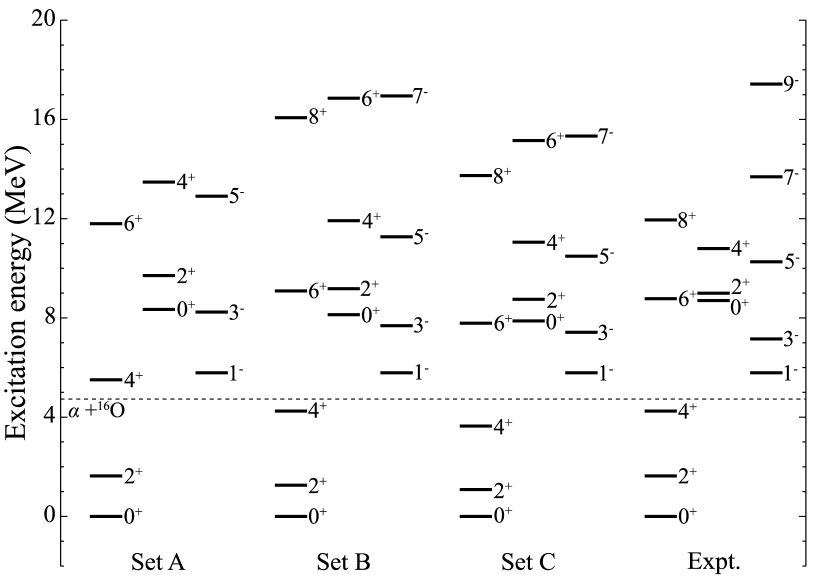
Figure 1: Energy spectrum of ²⁰Ne with three sets of $\alpha+^{16}$O potentials. Experimental data are taken from Ref. [43].

The calculated energy spectrum of ²⁰Ne is plotted in Fig. 1 together with the experimental data. The $J^{\pi}=0^{+},2^{+},$ and $4^{+}$ states are observed as bound states, and the other states including parity inverted states [42] are observed as resonant states. These levels are well recognized as the rotational structure of $\alpha+^{16}$O [42, 37]. The positive-parity higher nodal excited states of the ground-state band are also observed at $\gtrsim 8$ MeV. Here, the resonance energy $E_{R}$ is defined as an energy where the phase shift, $\delta_{J}$ crosses $\pi/2$. For a state with a broad width which does not reach $\delta_{J}=\pi/2$, we take a peak of the first derivative of the phase shift, $d\delta_{J}/dE$, as $E_{R}$. In Set A, where the $0^{+}$ and $2^{+}$ energies are used to fix the potential parameters, the $4^{+}$ state appears to be unbound and the other rotational levels tend to be at higher energy compared to the experimental data. Sets B and C show reasonable agreement with the observed spectrum for both the positive- and negative-parity states. The $0^{+},2^{+}$, and $4^{+}$ higher nodal excited states are also in fair agreement with the experimental data.

Table 2 summarizes the binding energies and decay widths of ²⁰Ne with the three sets of potential parameters. The decay widths are evaluated with $2/(d\delta_{J}/dE)|_{E=E_{R}}$. The observed decay widths are overestimated, with the best agreement for Set C. For the higher nodal states $J^{\pi}$, the calculated decay widths also tend to be larger than the experimental data. The fact is also found in the early $\alpha+^{16}$O OCM calculation [37], whose potential parameter is intermediate between Sets B and C.

Table 2: Energies and decay widths of ²⁰Ne with the $\alpha+^{16}$O model in MeV units. The energies are measured from the $\alpha+^{16}$O threshold. The lower rows list those of the nodal excited states of the ground-state band. Experimental data are taken from Ref. [43].

	Set A			Set B			Set C			Expt.
$J^{\pi}$	$E$	$\Gamma$		$E$	$\Gamma$		$E$	$\Gamma$		$E$	$\Gamma$
$0^{+}$	$-$4.730	–		$-$4.730	–		$-$4.730	–		$-$4.730	–
$2^{+}$	$-$3.096	–		$-$3.470	–		$-$3.649	–		$-$3.096	–
$4^{+}$	0.779	$<$3$\times 10^{-10}$		$-$0.482	–		$-$1.088	–		$-$0.482	–
$6^{+}$	7.07	2.0$\times 10^{-2}$		4.36	1.0$\times 10^{-3}$		3.06	6.2$\times 10^{-5}$		4.048	1.1$\times 10^{-4}$
$8^{+}$	16.22	0.17		11.34	3.5$\times 10^{-2}$		9.01	1.0$\times 10^{-2}$		7.22	3.5$\times 10^{-5}$
$1^{-}$	1.058	1.6$\times 10^{-5}$		1.058	3.4$\times 10^{-5}$		1.058	5.5$\times 10^{-5}$		1.058	2.8$\times 10^{-5}$
$3^{-}$	3.51	8.0$\times 10^{-2}$		2.96	5.0$\times 10^{-2}$		2.69	4.0$\times 10^{-2}$		2.426	8.2$\times 10^{-3}$
$5^{-}$	8.18	0.76		6.54	0.48		5.76	0.38		5.532	0.145
$7^{-}$	15.61	1.84		12.22	1.22		10.60	0.96		8.962	0.31
$9^{-}$	26.31	2.36		20.38	1.59		17.57	1.27		12.70	0.22
$0^{+}$	3.61	16.9		3.40	5.42		3.13	2.90		$\approx 4.0$	$>0.8$
$2^{+}$	4.98	18.6		4.45	6.76		4.02	3.84		4.27	$\approx 0.8$
$4^{+}$	8.75	21.0		7.19	9.05		6.32	5.60		6.07	0.35

Table 3: Point-matter rms radii and electric-quadrupole ($E2$) reduced transition probabilities of ²⁰Ne with the $\alpha+^{16}$O models. Three sets of potential parameters are employed. The point-proton rms radii of ⁴He and ¹⁶O are 1.455 and 2.568 fm, respectively, extracted from Ref. [39]. Values in parentheses are in units of W.u.$(=\frac{(1.2)^{2\lambda}}{4\pi}(\frac{3}{\lambda+3})^{2}A^{2\lambda/3}\ (e^{2}{\rm fm}^{2\lambda}$) [44]). The experimental $B(E2)$ value is taken from Ref. [43].

		Set A	Set B	Set C	Expt.
$r(0^{+})$ (fm)		2.768	2.840	2.889	2.889$\pm$0.002
$r(2^{+})$ (fm)		2.766	2.837	2.884
$r(4^{+})$ (fm)		unbound	2.827	2.872
$B(E2;2^{+}\to 0^{+})$ ($e^{2}$fm4)		30.2 (9.4)	43.9 (13.6)	54.7 (17.0)	65.5$\pm 3.2$ (20.3$\pm 1.0$)
$B(E2;4^{+}\to 2^{+})$ ($e^{2}$fm4)		–	58.4 (18.1)	72.2 (22.4)	71$\pm 6$ (22$\pm 2$)

Table 3 lists rms radii and reduced electric-quadrupole ($E2$) transition probabilities. The experimental data are also listed for comparison. The rms radius decreases with increasing angular momentum because the attractive pocket of the potential becomes narrower with increasing centrifugal barrier. Set C reproduces the $B(E2)$ value best among the three sets. Remarking that Set C is determined in such a way so as to reproduce the binding energy and the rms radius of the ground state of ²⁰Ne, the size of the ground-state wave function is essential to get a reasonable moment of inertia for describing the $\alpha+^{16}$O rotational structure in ²⁰Ne.

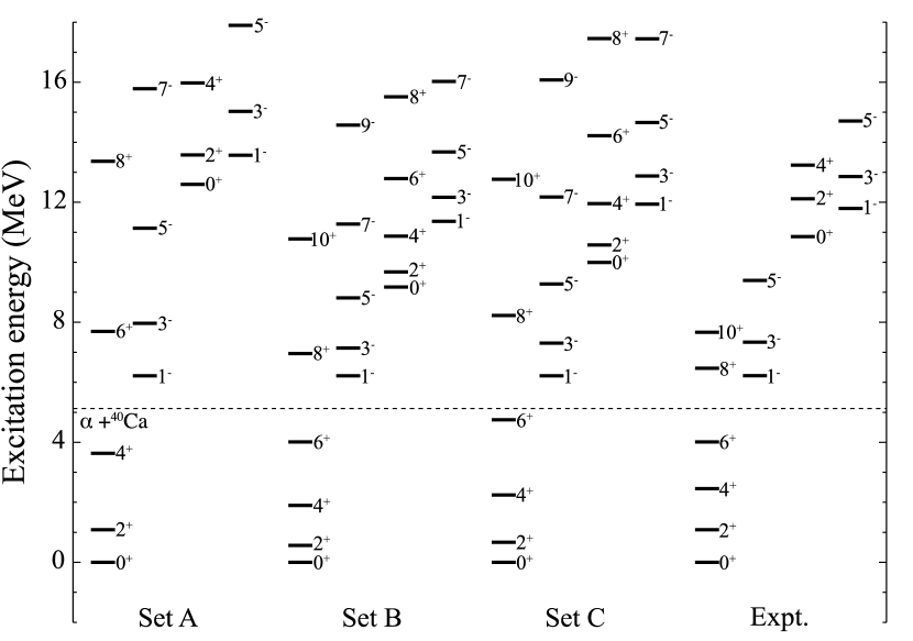
Figure 2: Energy spectrum of ⁴⁴Ti with three sets of $\alpha+^{40}$Ca potentials. Experimental data are taken from Ref. [45].

Table 4: Same as Table 3. but for ⁴⁴Ti with the $\alpha+^{40}$Ca model. The point-proton rms radius of ⁴⁰Ca is 3.377 fm extracted from Ref. [39]. The experimental $B(E2)$ value is taken from Ref. [45].

		Set A	Set B	Set C	Expt.
$r(0^{+})$ (fm)		3.437	3.548	3.515	3.515$\pm$0.005
$r(2^{+})$ (fm)		3.436	3.547	3.513
$r(4^{+})$ (fm)		3.434	3.542	3.509
$r(6^{+})$ (fm)		unbound	3.535	3.503
$B(E2;2^{+}\to 0^{+})$ ($e^{2}$fm4)		59.9 (6.5)	156.9 (17.0)	122.4 (13.3)	120$\pm 30$ (13$\pm 3$)
$B(E2;4^{+}\to 2^{+})$ ($e^{2}$fm4)		82.6 (8.9)	214.3 (23.2)	167.5 (18.1)	280$\pm 60$ (30$\pm 6$)
$B(E2;6^{+}\to 4^{+})$ ($e^{2}$fm4)		–	215.8 (23.4)	169.2 (18.3)	160$\pm 30$ (17$\pm 3$)

Table 5: Same as Table 2 but for ⁴⁴Ti with the $\alpha+^{40}$Ca model. Experimental data are taken from Ref. [45].

	Set A			Set B			Set C			Expt.
$J^{\pi}$	$E$	$\Gamma$		$E$	$\Gamma$		$E$	$\Gamma$		$E$
$0^{+}$	$-$5.127	–		$-$5.127	–		$-$5.127	–		$-$5.127
$2^{+}$	$-$4.044	–		$-$4.560	–		$-$4.457	–		$-$4.044
$4^{+}$	$-$1.496	–		$-$3.229	–		$-$2.883	–		$-$2.673
$6^{+}$	2.57	$<$5$\times 10^{-11}$		$-$1.112	–		$-$0.377	–		$-$1.112
$8^{+}$	8.24	4.5$\times 10^{-5}$		1.83	$<$2$\times 10^{-10}$		3.11	$<$1$\times 10^{-10}$		1.34
$10^{+}$	15.68	3.7$\times 10^{-3}$		5.65	6.3$\times 10^{-8}$		7.65	3.3$\times 10^{-6}$		2.54
$1^{-}$	1.093	$<$1$\times 10^{-12}$		1.093	$<$1$\times 10^{-12}$		1.093	$<$1$\times 10^{-12}$		1.093
$3^{-}$	2.84	2.9$\times 10^{-8}$		2.01	$\approx$5$\times 10^{-10}$		2.18	1.2$\times 10^{-9}$		2.21
$5^{-}$	6.01	6.2$\times 10^{-4}$		3.69	1.1$\times 10^{-5}$		4.15	3.2$\times 10^{-5}$		4.27
$7^{-}$	10.66	3.4$\times 10^{-2}$		6.14	1.5$\times 10^{-3}$		7.05	3.5$\times 10^{-3}$		–
$9^{-}$	16.93	0.22		9.45	1.8$\times 10^{-2}$		10.95	3.5$\times 10^{-2}$		–
$0^{+}$	7.47	1.20		4.05	1.2$\times 10^{-2}$		4.87	6.9$\times 10^{-2}$		5.73
$2^{+}$	8.45	1.70		4.55	2.6$\times 10^{-2}$		5.45	0.12		6.99
$4^{+}$	10.85	3.03		5.74	9.0$\times 10^{-2}$		6.83	0.29		8.11
$1^{-}$	8.44	8.22		6.24	2.48		6.81	3.38		6.67
$3^{-}$	9.90	10.2		7.04	2.99		7.75	4.08		7.73
$5^{-}$	12.77	13.2		8.55	3.84		9.53	5.21		9.58

Figure 2 displays the spectrum of ⁴⁴Ti. Similarly to the $\alpha+^{16}$O case, Set A produces a large moment of inertia resulting in too large an energy splitting between the intraband states, and Sets B and C fairly well reproduce the $\alpha+^{40}$Ca rotational structure [3, 46], that is, the low-lying positive- and negative-parity levels as well as their nodal excited states observed at $\gtrsim 12$ MeV, and the $B(E2)$ values as shown in Table 4. We also list, in Table 5, the binding energies and decay widths of ⁴⁴Ti with the $\alpha+^{40}$Ca model, although no $\alpha$-decay width is observed in such low-lying states.

5 Tests of the SUSY transformed potentials

Hereafter we employ Set C as the initial $\alpha$-nucleus deep potentials to be transformed by the SUSY prescription.

5.1 Physical properties of $\alpha+$nucleus systems

Table 6: Root-mean-square distances between the clusters, electric-quadrupole ($E2$) and hexadecapole ($E4$) reduced transition probabilities between the bound states. Both the results of ²⁰Ne and ⁴⁴Ti are listed.

20Ne		SUSY		SUSY-$\beta$		OCM
$\sqrt{\left<r^{2}\right>}(0^{+})$ (fm)		4.391		4.067		4.067
$\sqrt{\left<r^{2}\right>}(2^{+})$ (fm)		4.353		4.027		4.046
$\sqrt{\left<r^{2}\right>}(4^{+})$ (fm)		4.254		3.924		3.991
$B(E2;2^{+}\to 0^{+})$ (W.u.)		23.1		16.9		17.0
$B(E2;4^{+}\to 2^{+})$ (W.u.)		30.8		22.4		22.4
$B(E4;4^{+}\to 0^{+})$ (W.u.)		47.3		25.5		37.2
$B(E4;4^{+}\to 2^{+})$ (W.u.)		59.7		32.1		47.7
44Ti		SUSY		SUSY-$\beta$		OCM
$\sqrt{\left<r^{2}\right>}(0^{+})$ (fm)		5.157		4.657		4.657
$\sqrt{\left<r^{2}\right>}(2^{+})$ (fm)		5.132		4.631		4.642
$\sqrt{\left<r^{2}\right>}(4^{+})$ (fm)		5.071		4.569		4.607
$\sqrt{\left<r^{2}\right>}(6^{+})$ (fm)		4.967		4.463		4.547
$B(E2;2^{+}\to 0^{+})$ (W.u.)		20.0		13.3		13.3
$B(E2;4^{+}\to 2^{+})$ (W.u.)		27.5		18.2		18.1
$B(E2;6^{+}\to 4^{+})$ (W.u.)		28.3		18.5		18.3
$B(E4;4^{+}\to 0^{+})$ (W.u.)		53.6		23.7		36.7
$B(E4;4^{+}\to 2^{+})$ (W.u.)		68.4		30.3		47.4
$B(E4;6^{+}\to 2^{+})$ (W.u.)		76.0		33.2		51.1
$B(E4;6^{+}\to 4^{+})$ (W.u.)		58.4		25.4		40.7

Table 6 lists the rms distances between the clusters of the bound states with spin-parity $J^{\pi}=0^{+}$, $2^{+}$, 4⁺, reduced $E2$ and electric-hexadecapole ($E4$) transition probabilities of ²⁰Ne with the $\alpha+^{16}$O model. The relative wave functions between the clusters are generated by the SUSY transformed potentials as well as the initial deep OCM potential. Despite the fact that the SUSY and deep potentials give exactly the same phase shift, the rms distances and the $B(E2)$ values are actually modified and increased by the standard SUSY transformation. Those observables are somewhat sensitive to the wave function at short distances. On the contrary, the changes in the $B(E4)$ values are relatively smaller than that of the $B(E2)$ case. Since the operator is proportional to $r^{4}$, the $B(E4)$ values are less sensitive to the internal regions of the wave function, whereas the external regions contribute largely to the $B(E4)$ matrix element. Recalling that we fix the parameters of the deep potential in such a way so as to reproduce the binding energy and rms radius of the ground-state wave function of ²⁰Ne, the standard SUSY transformation is no longer a desired potential.

Therefore, we consider another SUSY transformation (SUSY-$\beta$) prescribed in Sec. 2.2 with the arbitrary parameter $\beta$ being fixed so as to reproduce the rms radius of the ground state. The choice of the $\beta$ value can be angular-momentum dependent. We, however, transform all the $J^{\pi}$ states having the physical bound states with the same $\beta$ value for the sake of simplicity. The $\beta$ values are $-1.8670$ and $-1.3791$ for ²⁰Ne and ⁴⁴Ti, respectively. These values are negative in order to provide a narrower pocket in the potential. As shown in Table 6, the $B(E2)$ values and rms radii of the bound $2^{+}$ and $4^{+}$ states are remedied by this transformation. However, the $B(E4)$ value shows some deviation from that with the OCM calculation. We will return to this matter later in Sec. 5.3.

The same holds for ⁴⁴Ti. Table 6 also lists rms distances between the clusters, reduced $E2$, $E4$ transition probabilities of ⁴⁴Ti in the $\alpha+^{40}$Ca potential models. As already seen in the ²⁰Ne case, the rms distances and $B(E\lambda)$ transition probabilities are modified by the standard SUSY transformation. The modification becomes somewhat moderate for higher multipoles due to the $r^{\lambda}$ factor in the electric-multipole operator with a rank $\lambda$. In fact, similarly to the ²⁰Ne case, the SUSY-$\beta$ transformation gives smaller $B(E4)$ values. Though one always needs to check how observables of interest are modified by the transformation, as long as the rms radius and $B(E2)$ values are of interest, the SUSY-$\beta$ seems to provide a reasonable forbidden-state-free potential which can be used for studying more than three-cluster systems.

5.2 Supersymmetric transformed potentials and wave functions

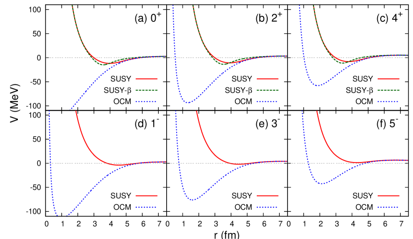
Figure 3: Comparison of the SUSY transformed and original deep (OCM) potentials of the $\alpha+^{16}$O system for the $J^{\pi}=$ (a) 0⁺, (b) 2⁺, (c) 4⁺, (d) 1^-, (e) 3^-, and (f) 5^- states. The Coulomb and centrifugal potentials are included in the plot. Set C potential is employed.

Figure 3 plots the SUSY transformed $\alpha+^{16}$O potentials as well as the original deep potential for different $J^{\pi}$ states. The Coulomb and centrifugal potentials are included in the plots. No SUSY-$\beta$ potential exists for the negative parity states as they have no physical bound state.

The SUSY transformed potentials at $r\lesssim 5$ fm behave quite differently from the original deep potential. For all the $J^{\pi}$ states, including the $0^{+}$ state, we see a strong repulsion for $r\lesssim 3$ fm generated from the SUSY transformations pushing the internal wave function to outer regions. This behavior is a general consequence of removing the redundant bound states while keeping the phase shift invariant. We see attractive pockets at $\sim 4$ fm for the $0^{+}$, $2^{+}$, and $4^{+}$ states which allow us to obtain one physical bound-state solution. The attractive pocket is somewhat shifted to inner regions with the SUSY-$\beta$ transformation with a negative $\beta$ value because this transformation always gives a smaller rms radius than that of the standard SUSY transformation shown in Table 6.

For the negative-parity partial waves, the pocket is not deep enough to accommodate any bound state. The lowest state appears as a resonance with a narrow width. We again remark that all the potentials give exactly the same phase shift.

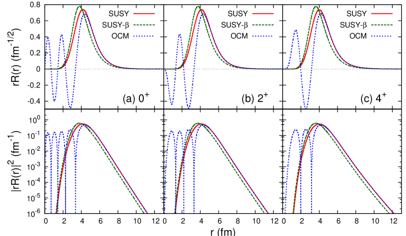
Figure 4: Comparison of the bound-state wave functions of the lowest (a) 0⁺, (b) $2^{+}$, and (c) $4^{+}$ physical states of ²⁰Ne obtained with the SUSY transformed and the original deep (OCM) potentials.

We solve the Schrödinger equation numerically for each $J$ with those potentials. The second-order differential equation is precisely solved by a finite-difference method, the Numerov method, with the boundary condition that the logarithmic derivative of the numerical wave function matches the Whittaker function [47, 38] at large distances. Figure 4 plots the radial wave function of physical bound states of ²⁰Ne generated by the SUSY transformed and original deep potentials. Logarithmic plots of the probability distribution are also presented in order to clearly see the asymptotics of the wave functions. When the OCM calculation is made, all the displayed physical wave functions obtained with the deep potential exhibit several nodes that satisfy the total harmonic-oscillator quanta $Q=2n_{r}+l=8$ and the internal wave function $r\lesssim 4$ fm changes drastically with the angular momentum increases. In contrast, the SUSY transformed potentials provide nodeless wave functions for these physical bound states, and the behavior of the wave functions in the internal regions does not depend so much on the angular momentum. As seen in Fig. 4, the wave functions obtained by the original deep and standard SUSY transformed potentials are identical for $r\gtrsim 5$ fm, which can be expected from the phase-equivalence. The SUSY-$\beta$ potential also gives a nodeless wave function but the peak position is a little shifted to the inner regions corresponding to the position of the attracted potential pocket as already seen in Fig. 3. Each SUSY-$\beta$ wave function shows the same decrease asymptotically but its asymptotic normalization coefficient is different from the others as explained by Eq. (6).

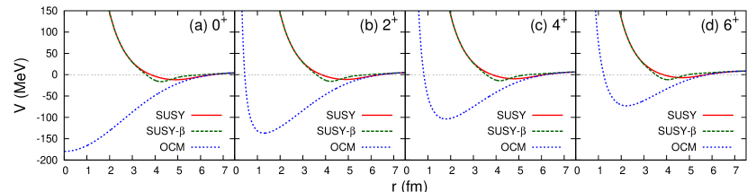
Figure 5: Same as Fig. 3 but for the lowest $J^{\pi}=$ (a) 0⁺, (b) 2⁺, (c) 4⁺, and (d) 6⁺ physical states of the $\alpha+^{40}$Ca system.

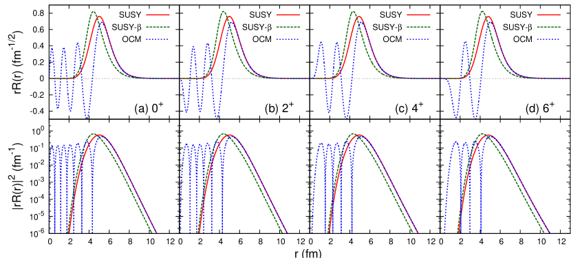
Figure 6: Same as Fig. 4 but with the lowest (a) 0⁺, (b) 2⁺, (c) 4⁺, and (d) $6^{+}$ physical states of ⁴⁴Ti.

We also display the $\alpha+^{40}$Ca potentials in Fig. 5. More singular potentials around the origin are obtained for the $\alpha+^{40}$Ca system because the number of forbidden states ($Q=2n_{r}+l<12$) is larger than that of ²⁰Ne, and more transformations are needed to remove all these forbidden states. Figure 6 plots the wave functions and probability distributions for the lowest $J^{\pi}=0^{+}$, $2^{+}$, $4^{+}$, and $6^{+}$ physical states of ⁴⁴Ti. As expected, two more nodes with respect to the ²⁰Ne case appear in the wave function obtained with the OCM calculation. Though there is a little difference in the wave functions, the same discussion given for the $\alpha+^{16}$O system holds for the asymptotic behavior of the wave function with the SUSY and SUSY-$\beta$ transformations.

5.3 Electric-multipole transition densities

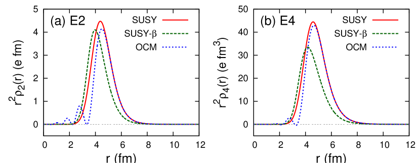
Figure 7: Transition densities of the electric- (a) quadrupole ($E2$) and (b) hexadecapole ($E4$) operators of ²⁰Ne from the $0^{+}$ ground state to the yrast $2^{+}$ and $4^{+}$, respectively, obtained with the SUSY transformed and original deep (OCM) potentials.

In order to clearly see where the electric multipole transitions occur, we evaluate the transition densities, which show the spatial distribution of the electric-multipole ($E\lambda$) transition matrix elements, defined by

$$\rho_{\lambda}(E,r)=\int d\hat{\bm{r}}\,[\Psi_{\lambda\mu}(E,\bm{r})]^{*}\mathcal{M}_{\lambda\mu}\Psi_{00}(E_{0},\bm{r})$$ (13)

with the relation to the transition matrix element as

$$\int_{0}^{\infty}dr\,r^{2}\rho_{\lambda}(E,r) =\frac{1}{\sqrt{2\lambda+1}}\left<\Psi_{\lambda}(E)\|\mathcal{M}_{\lambda}\|\Psi_{0}(E_{0})\right>.$$ (14)

Figure 7 plots the $E\lambda$ transition densities from the ground state to the positive-parity bound $J^{\pi}=2^{+}$ and $4^{+}$ states of ²⁰Ne. As expected from the behavior of the phase-equivalent wave functions shown in Fig. 4, the transition densities generated from the SUSY and original deep potentials are almost identical beyond $\sim 5$ fm, whereas the SUSY-$\beta$ result is quite different from the others. Due to the $r^{\lambda}$ factor in the electric-multipole operators, the difference below $\sim 5$ fm becomes smaller with higher $\lambda$. Here we can see the reason why the SUSY-$\beta$ gives the smaller $E4$ values listed in Table 6. We remark that the SUSY-$\beta$ transformation reduces the amplitude of the wave function in the asymptotic regions shown in Fig.4, and the contributions of the $E4$ transitions are dominated by the outer regions of the wave function. Therefore, the $E4$ values become much smaller then those of the OCM by the SUSY-$\beta$ transformation.

5.4 Tests in electric-multipole strength functions and cluster sum rules

To further study the possible modifications of observables by the SUSY transformations, we calculate electric-multipole ($E\lambda$) strength functions. Here we do not show the results of ⁴⁴Ti because the same discussions as the ²⁰Ne case can be made. The $E\lambda$ strength function is defined by

$$S(E\lambda;E)=\mathcal{S}_{f\mu}\left|\left<\Psi_{\lambda\mu}(E_{f})|\mathcal{M}_{\lambda\mu}|\Psi_{00}(E_{0})\right>\right|^{2}\delta(E_{f}-E),$$ (15)

where $\mathcal{S}_{f\mu}$ denotes a sum over the $2\lambda+1$ $\mu$ values and the final state energy $E_{f}$. The final state continuum wave function is normalized as

$$\int[\Psi_{\lambda\mu}(E^{\prime},\bm{r})]^{*}\Psi_{\lambda\mu}(E,\bm{r})d\bm{r}=\delta(E-E^{\prime}),$$ (16)

which is practically achieved by connecting the numerical solution to the asymptotic Coulomb wave function with the wave number $k=\sqrt{2mE}/\hbar$ according to

$$\chi(r)\to\sqrt{\frac{2m}{\pi\hbar^{2}k}}[\cos{\delta_{J}}F_{J}(kr)+\sin{\delta_{J}}G_{J}(kr)],\quad(r\to\infty)$$ (17)

where $\delta_{J}$ is a phase shift, $F_{J}(G_{J})$ is a regular (irregular) Coulomb function [38].

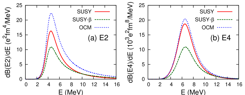
Figure 8: Transition strengths of (a) electric-quadrupole ($E2$) and (b) hexadecapole ($E4$) operators of ²⁰Ne obtained with the SUSY transformed and original deep (OCM) potentials.

Figure 8 plots the $E2$ and $E4$ strength functions of ²⁰Ne As expected, the OCM and SUSY results become closer with increasing multipolarity $\lambda$ because contributions of the asymptotic regions become more important. We also calculate the monopole strength function with the operator $M_{00}=\frac{A_{1}A_{2}}{A}r^{2}$ which allows us to populate the nodal excited $0^{+}$ states. Since the operator is proportional to $r^{2}$, the behavior of the transition strengths is similar to that of $E2$ shown in Fig. 8(a).

Figure 9 plots the transition densities at the peak positions for the higher nodal $J^{\pi}=2^{+}$ and $4^{+}$ states that were observed as broad resonances [43]. The transition densities obtained with the original deep and SUSY potentials are identical beyond $\sim 5$ fm. The difference in the transition densities is only found in the internal regions below $\sim 5$ fm and becomes smaller with increasing $\lambda$. In the previous subsection, we discussed the case where the final state is bound or a sharp resonance. In this case, the overlap of the initial wave function multiplied by the $E\lambda$ operator is still large even at short distances. Here we discuss transitions to the continuum or a broad resonant state. The effects of the internal wave function is much smaller because the final state wave function is more extended and displays less amplitude in the internal regions. The SUSY-$\beta$ transformation always gives smaller strengths than the others because it reduces the amplitude of the asymptotic wave function.

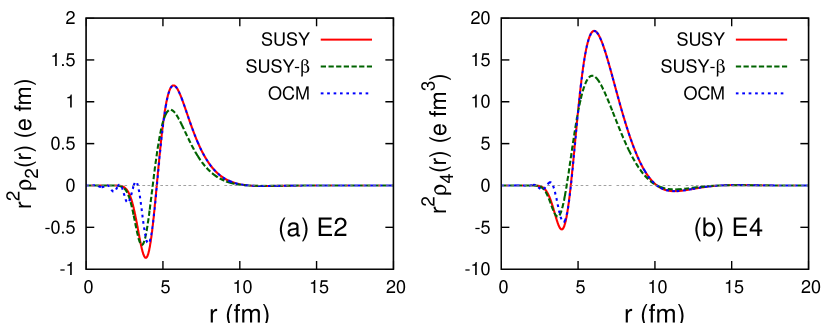
Figure 9: Same as Fig. 7 but to the higher nodal states which show the second largest transition strengths for each $J^{\pi}$.

Finally, we discuss the electric-multipole sum rules. The non-energy-weighted-cluster sum rules of the $E\lambda$ transitions are defined by

$$m_{0}(E\lambda)=\int_{-\infty}^{\infty}S(E\lambda,E^{\prime})\,dE^{\prime}=m_{0}^{\rm A}(E\lambda)+m_{0}^{\rm F}(E\lambda)$$ (18)

with the calculable expressions

$$m_{0}(E\lambda) =\sum_{\mu}\left<\Psi_{00}(E_{0})\right|\mathcal{M}_{\lambda\mu}^{\dagger}\mathcal{M}_{\lambda\mu}\left|\Psi_{00}(E_{0})\right>,$$ (19)

$$m_{0}^{\rm F}(E\lambda) =\sum_{i=1}^{n}\sum_{\mu}\left|\left<\phi^{\rm F}_{\lambda\mu}(E^{\rm F}_{i})\right|\mathcal{M}_{\lambda\mu}\left|\Psi_{00}(E_{0})\right>\right|^{2},$$ (20)

where $\phi^{\rm F}_{\lambda\mu}(E_{i}^{\rm F})$ denotes the wave function of the forbidden state with the energy $E_{i}^{\rm F}$. Note that the sum rule is generalized and consists of contributions from allowed ($m_{0}^{\rm A}$) and forbidden ($m_{0}^{\rm F}$) states. It is obvious that $m_{0}^{\rm F}$ is zero with use of the SUSY transformed potentials. Some strengths are distributed to the redundant bound states when the deep potential is employed.

Table 7 lists the sum-rule values with the $E2$ and $E4$ operators obtained by the different potential models. Those values are dominated by $m_{0}^{\rm A}$. The $m_{0}^{\rm F}$ contributions to the total sum rule are small. To better quantify the modifications by the SUSY transformations, we also list the ratios to the value obtained by the OCM calculation in parentheses. The $m_{0}^{\rm A}$ values with the SUSY potential approach unity with increasing $\lambda$ due to $r^{2\lambda}$ factor in Eq. (19). In contrast, the sum-rule ratios with the SUSY-$\beta$ potential decrease with increasing multipolarity because the contributions from the asymptotic regions become more important with higher multipolarity and the amplitude of the asymptotic wave function becomes smaller than that of the original one as already seen in Fig. 4.

Table 7: Non-energy-weighted-cluster-electric-multipole ($E\lambda$) sum rules of ²⁰Ne in units of W.u.. Values in parentheses are the ratios to the value obtained by the OCM.

			SUSY		SUSY-$\beta$		OCM
$E2$	$m_{0}$		133.4 (1.13)		98.9 (0.835)		118.5
	$m_{0}^{\rm A}$		133.4 (1.18)		98.9 (0.873)		113.2
	$m_{0}^{\rm F}$		–		–		5.26
$E4$	$m_{0}$		810.4 (1.04)		471.1 (0.606)		777.8
	$m_{0}^{\rm A}$		810.4 (1.06)		471.1 (0.617)		763.3
	$m_{0}^{\rm F}$		–		–		14.6

6 Conclusion

Deep potentials can simulate the interaction of two clusters but are practically hard to apply to few-body models of multi-cluster systems. It is possible to replace these potentials by phase-equivalent shallow potentials with the same physical bound states, which are simpler to use. The wave functions are however modified. In this work, we have quantified this effect with physical properties, i.e., electric transition probabilities.

Towards the application of a macroscopic cluster model to systems involving heavy clusters, we have introduced phenomenological deep $\alpha+^{16}$O and $\alpha+^{40}$Ca potentials which accommodate several redundant bound states. We found that, in order to understand the excitation spectrum as well as the electric-quadrupole transitions of ²⁰Ne and ⁴⁴Ti, it is essential for the inter-cluster potential to reproduce the ground-state energy and root-mean-square (rms) radius.

Since it is hard to apply this potential directly to multi-cluster systems, we remove the unphysical forbidden states by using supersymmetric (SUSY) transformations. We have tested the relative wave functions generated by the SUSY transformed potentials in comparison with the ones generated by the original deep potentials. Though the SUSY transformed potentials give exactly the same phase shift as the original one, some observables which are sensitive to the wave function at short distances (e.g., the rms radius and electric-quadrupole transition probabilities) are unfavorably modified. Therefore, we introduce another SUSY transformation (SUSY-$\beta$) involving one arbitrary parameter which is determined in such way so as to reproduce the rms radius obtained by the original wave function.

To quantify the modification caused by the SUSY transformations, we study the electric-multipole ($E\lambda$) transitions. The modification due to the standard SUSY transformation becomes relatively smaller with increasing multipolarity $\lambda$ due to the $r^{\lambda}$ factor in the $E\lambda$ operator. By applying the SUSY-$\beta$ transformation which keeps the rms radius invariant, the initial value of the $E2$ transition strengths is recovered. However, the observables with higher multipolarity, e.g., $E4$, are too strongly reduced because the single arbitrary parameter included in the transformation reduces the amplitude of the asymptotic wave function.

The SUSY prescription offers a phase-equivalent singular-shallow potential consistent with the deep potential. Such a potential is advantageous for descriptions of multi-cluster systems. However, we should keep in mind that some observables are possibly modified by the transformation. The standard SUSY transformation modifies observables which are sensitive to the wave functions at short distances. The modification may be partly recovered by another SUSY transformation modifying a bound state, i.e. we can “design” the singular-shallow potential. But again, one needs to care about the modification of the other observables that are sensitive to the amplitude of the asymptotic regions. To further test the potential models presented in this paper, it is interesting to apply them to macroscopic three-cluster systems such as ²¹Ne (²¹Na)$=^{16}$O$+\alpha+n$ ($p$), and ²⁴Mg$=^{16}$O$+\alpha+\alpha$ systems as well as systems involving $\alpha$ and ⁴⁰Ca clusters. These applications will verify the validity of the potential models through comparison with experimental data.

References

References

- [1] K. Ikeda, N. Takigawa, H. Horiuchi, The Systematic Structure-Change into the Molecule-like Structures in the Self-Conjugate Nuclei, Prog. Theor. Phys. Suppl. E68 (1968) 464.
- [2] Y. Fujiwara, H. Horiuchi, K. Ikeda, M. Kamimura, K. Katō, Y. Suzuki, E. Uegaki, Chapter II. Comprehensive Study of Alpha-Nuclei, Prog. Theor. Phys. Suppl. No. 68 (1980) 29.
- [3] F. Michel, S. Ohkubo, G. Reidemeister, Local Potential Approach to the Alpha-Nucleus Interaction and Alpha-Cluster Structure in Nuclei, Prog. Theor. Phys. Suppl. 132, (1998) 7, and references therein.
- [4] Clusters in Nuclei, Volume 1 (2010); 2 (2012); and 3 (2014), edited by C. Beck, Springer (Berlin), and references theirin.
- [5] M. Kamimura, Transition densities between the , , , , , and states in 12C derived from the three-alpha resonating-group wave functions, Nucl. Phys. A351 (1981) 456.
- [6] Y. Suzuki, Structure Study of States in 16O by 12C Cluster-Coupling Model. I, Prog. Theor. Phys. 55 (1976) 1751.
- [7] Y. Suzuki, Structure Study of States in 16O by 12C Cluster-Coupling Model. II, Prog. Theor. Phys. 56 (1976) 111.
- [8] F. Hoyle, On Nuclear Reactions Occurring in Very Hot STARS.I. the Synthesis of Elements from Carbon to Nickel, Astrophys. J. Suppl. Ser. 1 (1954) 121.
- [9] J.A. Wheeler, Molecular Viewpoints in Nuclear Structure, Phys. Rev. 52 (1937) 1083.
- [10] J.A. Wheeler, On the Mathematical Description of Light Nuclei by the Method of Resonating Group Structure, Phys. Rev. 52 (1937) 1107.
- [11] K. Wildermuth and W. McClure, Cluster Representation of Nuclei, Springer Tracts in Modern Physics 41 (1966) 1.
- [12] N. Itagaki, A. Ohnishi, K. Katō, Microscopic -Cluster Model for 12C and 16O Based on Antisymmetrized Molecular Dynamics: Consistent Understanding of the Binding Energies of 12C and 16O, Prog. Theor. Phys. 94 (1995) 1019.
- [13] S. Saito, Effect of Pauli Principle in Scattering of Two Clusters, Prog. Theor. Phys. 40 (1968) 893.
- [14] S. Saito, Interaction between Clusters and Pauli Principle, Prog. Theor. Phys. 41 (1969) 705.
- [15] S. Saito, Chapter II. Theory of Resonating Group Method and Generator Coordinate Method, and Orthogonality Condition Model, Prog. Theor. Phys. Suppl. 62 (1977) 11.
- [16] B. Buck, H. Friedrich, C. Wheatley, Local potential models for the scattering of complex nuclei, Nucl. Phys. A275 (1977) 246.
- [17] V.I. Kukulin and V.N. Pomerantsev, The orthogonal projection method in scattering theory, Ann. Phys. 111 (1978) 330.
- [18] M. Theeten, D. Baye, P. Descouvemont, Comparison of local, semi-microscopic, and microscopic three-cluster models, Phys. Rev. C 74 (2006) 044304.
- [19] Y. Funaki, T. Yamada, H. Horiuchi, G. Röpke, P. Schuck, A. Tohsaki, -Particle Condensation in 16O Studied with a Full Four-Body Orthogonality Condition Model Calculation, Phys. Rev. Lett. 101 (2008) 082502.
- [20] E. Hiyama, M. Kamimura, Y. Yamamoto, T. Motoba, Five-Body Cluster Structure of the Double- Hypernucleus Be, Phys. Rev. Lett. 104 (2010) 212502.
- [21] W. Horiuchi and Y. Suzuki, Correlated-basis description of -cluster and delocalized states in 16O, Phys. Rev. C 89 (2014) 011304(R).
- [22] S. Ali and A.R. Bodmer, Phenomenological - potentials, Nucl. Phys. 80 (1966) 99.
- [23] E.M. Tursunov, D. Baye, P. Descouvemont, Comparative variational studies of states in three- models, Nucl. Phys. A723 (2003) 365.
- [24] S. Ishikawa, Three-body calculations of the triple- reaction, Phys. Rev. C 87 (2013) 055804.
- [25] H. Suno, Y. Suzuki, P. Descouvemont, Triple- continuum structure and Hoyle resonance of 12C using the hyperspherical slow variable discretization, Phys. Rev. C 91 (2015) 014004.
- [26] D. Baye, Supersymmetry between deep and shallow nucleus-nucleus potentials, Phys. Rev. Lett. 58 (1987) 2738.
- [27] D. Baye and J.-M. Sparenberg, Inverse scattering with supersymmetric quantum mechanics, J. Phys. A: Math. Gen. 37 (2004) 10223.
- [28] D. Baye, J.-M. Sparenberg, A. M. Pupasov, B. F. Samsonov, Single- and coupled-channel radial inverse scattering with supersymmetric transformations, J. Phys. A: Math. Theor. 47 (2014) 243001.
- [29] P. Swan, Asymptotic phase-shifts and bound states for two-body central interactions, Nucl. Phys. 46 (1963) 669.
- [30] P. Swan, The exclusion principle and equivalent potentials for scattering of complex neutral particles, Ann. Phys. NY 48 (1968) 455.
- [31] Y. Suzuki, H. Matsumura, M. Orabi, Y. Fujiwara, P. Descouvemont, M. Theeten, D. Baye, Local versus nonlocal interactions in a description of 12C, Phys. Lett. B659 (2008) 160.
- [32] E.C. Pinilla, D. Baye, P. Descouvemont, W. Horiuchi, Y. Suzuki, Tests of the discretized-continuum method in three-body dipole strengths, Nucl. Phys. A865 (2011) 43.
- [33] D. Baye, Phase-equivalent potentials from supersymmetry, J. Phys. A: Math. Gen. 20 (1987) 5529.
- [34] C.V. Sukumar, Supersymmetric quantum mechanics of one-dimensional systems, J. Phys. A: Math. Gen. 18 (1985) 2917.
- [35] W. Horiuchi and Y. Suzuki, Tests of a Deformable Core Plus Few-Nucleon Model, Few-Body Syst. 55 (2014) 121.
- [36] D. Baye and E.M. Tursunov, Isospin-forbidden electric-dipole capture and the Li reaction, arXiv: 1710.06352.
- [37] A.T. Kruppa and K. Katō, Resonances in Complex-Scaled Orthogonality Condition Model of Nuclear Cluster System, Prog. Theor. Phys. 84 (1990) 1145.
- [38] M. Abramowitz and I.A. Stegun, Handbook of Mathematical Functions with Formulas, Graphs, Mathematical Tables, Dover, Mineola, NY (1970).
- [39] I. Angeli and K.P. Marinova, Table of experimental nuclear ground state charge radii: An update, Atomic Data and Nuclear Data Tables 99 (2013) 69.
- [40] W.J. Huang, G. Audi, M. Wang, F.G. Kondev, S. Naimi, X. Xu, The AME2016 atomic mass evaluation (I). Evaluation of input data; and adjustment procedures, Chin. Phys. C 41 (2017) 030002.
- [41] M. Wang, G. Audi, F.G. Kondev, W.J. Huang, S. Naimi, X. Xu, The AME2016 atomic mass evaluation (II). Tables, graphs and references, Chin. Phys. C 41 (2017) 030003.
- [42] H. Horiuchi and K. Ikeda, A Molecule-like Structure in Atomic Nuclei of 16O∗ and 10Ne, Prog. Theor. Phys. 40 (1968) 277.
- [43] D.R. Tilley, C.M. Cheves, J.H. Kelley, S. Raman, H.R. Weller, Energy levels of light nuclei, , Nucl. Phys. A636 (1998) 249.
- [44] A. Bohr and B.R. Mottelson, Nuclear Structure, Vol. I, W.A. Benjamin, New York (1975).
- [45] J. Chen, B. Singh, J.A. Cameron, Nuclear Data Sheets for , Nucl. Data Sheets 112 (2011) 2357.
- [46] M. Kimura and H. Horiuchi, Coexistence of cluster structure and superdeformation in 44Ti, Nucl. Phys. A767 (2006) 58.
- [47] E.T. Whittaker, G.N. Watson, A Course of Modern Analysis, Fourth edition, Cambridge Univ. Press, Cambridge (1927).