Mixing and perfect sampling in one-dimensional particle systems

Abstract

We study the approach to equilibrium of the event-chain Monte Carlo (ECMC) algorithm for the one-dimensional hard-sphere model. Using the connection to the coupon-collector problem, we prove that a specific version of this local irreversible Markov chain realizes perfect sampling in $\mathcal{O}({N^{2}\log N})$ events, whereas the reversible local Metropolis algorithm requires $\mathcal{O}({N^{3}\log N})$ time steps for mixing. This confirms a special case of an earlier conjecture about $\mathcal{O}({N^{2}\log N})$ scaling of mixing times of ECMC and of the forward Metropolis algorithm, its discretized variant. We furthermore prove that sequential ECMC (with swaps) realizes perfect sampling in $\mathcal{O}({N^{2}})$ events. Numerical simulations indicate a cross-over towards $\mathcal{O}({N^{2}\log N})$ mixing for the sequential forward swap Metropolis algorithm, that we introduce here. We point out open mathematical questions and possible applications of our findings to higher-dimensional statistical-physics models.

1 Sampling, mixing, perfect sampling, stopping rules

Ever since the 1950s[1], Markov-chain Monte Carlo (MCMC) methods have ranked among the most versatile approaches in scientific computing. Monte Carlo algorithms strive to sample a probability distribution $\pi^{()}$. For an $N$-particle system in statistical mechanics, with particle $i\in\{1,\ldots,N\}$ described by coordinates $x_{i}$, sampling $\pi$ corresponds to generating configurations $\mathbf{x}=\{x_{1},\ldots,x_{N}\}$ distributed with the Boltzmann probability $\pi^{()}(\mathbf{x})\propto\exp\left[-\beta E(\mathbf{x})\right]$, where $E$ is the system energy and $\beta$ the inverse temperature. For problems where $\mathbf{x}$ lies in a high-dimensional discrete or continuous space $\Omega$, this sampling problem can usually not be solved directly [2, 3].

MCMC consists instead in sampling a probability distribution $\pi^{(t)}$ that evolves with a time $t$. The initial probability distribution, at time $t=0$, $\pi^{(t=0)}$, can be sampled directly. Often, it is simply composed of a single configuration, so that $\pi^{(0)}$ is a $\delta$-function on an explicitly given configuration $\{x_{1},\ldots,x_{N}\}$. In the limit $t\to\infty$, the distribution $\pi^{(t)}$ evolves from the initial one towards the target probability distribution $\pi^{()}=\lim_{t\to\infty}\pi^{(t)}$. Besides the development of MCMC algorithms that approach the limit distribution $\pi^{()}$ as quickly as possible for any initial distribution $\pi^{(0)}$, a key challenge in MCMC consists in estimating the time scale on which the time-dependent distribution $\pi^{(t)}$, which depends on $\pi^{(0)}$, is sufficiently close to $\pi^{()}$ that the two agree for all intents and purposes. This program has met with considerable success in some models of statistical physics, for example for the local Glauber dynamics in the two-dimensional Ising model [4, 5].

The difference between two (normalized) probability distributions $\pi^{()}$ and $\tilde{\pi}^{()}$ is often quantified by the total variation distance (TVD) [6, 7],

which satisfies $0\leq\|\tilde{\pi}^{()}-\pi^{()}\|_{\text{TV}}\leq 1$. The mixing time, the most relevant figure of merit for a Monte Carlo algorithm, is defined as the time $t$ after which the TVD (with $\tilde{\pi}^{()}\equiv\pi^{(t)}$ in eq. (LABEL:equ:SecondDefinitionTVD)) is smaller than a given threshold $\epsilon$, for any initial distribution $\pi^{(0)}$. Although it is of great conceptual importance, the TVD cannot usually be computed. In statistical physics, this is already because the normalization of the Boltzmann weight, the partition function $Z=\int_{\Omega}\exp\left(-\beta E\right)$, is most often unknown. Also, the distribution $\pi^{(t)}(\mathbf{x})$ is not known explicitly. It is because of this difficulty that practical simulations often carry systematic uncertainties that are difficult to quantify, and that heuristic convergence criteria for the approach towards equilibrium in MCMC abound[8, 9, 3]. They most often involve time-correlation functions of observables, rather than the probability distribution itself (as in eqs (LABEL:equ:FirstDefinitionTVD) and (LABEL:equ:SecondDefinitionTVD)).

In rare cases, MCMC algorithms allow for the definition of a stopping rule (based on the concept of a strong stationary time[6]), that yields a simulation-dependent value of $t$ at which the configuration is sampled exactly from the distribution $\pi^{()}$. The value of $t$ now often depends on the realization of the Markov chain (that is, on the individual sampled moves and, ultimately, on the drawn random numbers). The framework of stopping rules can be used to bound the mixing time[6]. Stopping rules exist for quite intricate models, as for example the Ising model, using the mixing-from-the-past framework[10, 3].

The great majority of Markov-chain Monte Carlo algorithms are reversible (they satisfy the detailed-balance condition). This is the case for example for all algorithms that are based on the Metropolis or the heat-bath algorithms[1, 3], which allow reversible MCMC algorithms to be readily constructed for any distribution $\pi^{()}$, that is, for an arbitrary energy $E(\mathbf{x})$. In recent years, however, irreversible MCMC methods based on the global balance condition have shown considerable promise[11, 12, 13, 14, 15]. In these algorithms, $\pi^{(t)}$ approaches $\pi^{()}$ for long times, but the flows no longer vanish. One particular irreversible Markov chain, the event-chain Monte Carlo (ECMC) algorithm[13, 14], has proven useful for systems ranging from hard-sphere models[16] to spin systems[17], polymers[18, 19] and to long-range interacting ensembles of molecules, such as water[20], where the Coulomb interaction plays a dominant role[21]. Although there have been many indications of the algorithm’s power, no exact results were known for the mixing behavior of ECMC, except for the case of a single particle, $N=1$ [22].

In the present paper, we rigorously establish ECMC mixing times and stopping rules of the model of $N$ hard spheres on a one-dimensional line with periodic boundary conditions (a circle). Reversible MCMC algorithms for this model and its variants were analyzed rigorously[23, 24] and irreversible MCMC algorithm were discussed in detail[15]. The 1D hard-sphere model and reversible and irreversible MCMC algorithms are closely related to the symmetric exclusion process (SEP) on a periodic lattice[25] and to the totally asymmetric simple exclusion process (TASEP) [26, 27, 28]. For ECMC, an algorithm that is closely related to the lifted Metropolis algorithm[15], we compute the TVD in a special case, and obtain the mixing times as a function of the parameter $\epsilon$. We confirm the $\mathcal{O}({N^{2}\log N})$ mixing time that had been conjectured on the basis of numerical simulations[15]. Furthermore, we obtain a stopping rule for ECMC. We moreover present sequential variants of the forward Metropolis algorithm and the ECMC algorithm. For the latter, we prove an $\mathcal{O}({N^{2}})$ exact-sampling result that seems however not to generalize the discretized version of the algorithm.

2 Hard spheres in 1D, reversible Monte Carlo

The mixing and convergence behavior of Markov chains for particle systems has been much studied. As for hard spheres in 2D and above, phase transitions have only been identified by numerical simulation[29, 30, 16], it is natural that few rigorous results are available for the convergence and mixing behavior of MCMC algorithms in $D>1$[31, 32]. We thus restrict our attention to the 1D hard-sphere model with periodic boundary conditions and treat both the discrete and the continuous cases.

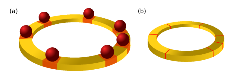
Figure 1: 1D hard-sphere model with periodic boundary conditions. (a): $N$ spheres of diameter $d$ on a ring of length $L$. (b): $N$ point particles on a ring of length $L_{\text{free}}=L-Nd$. Configurations and local MCMC algorithms are equivalent for both representations.

The 1D hard-sphere model can be represented as $N$ spheres of diameter $d$ on a line of length $L$ with periodic boundary conditions (that is, on a ring, see Fig. 1a). A valid configuration $a$ of $N$ spheres has unit statistical weight $\pi(a)=1$. Spheres do not overlap, so that the distance between sphere centers, and in particular between neighboring spheres, is larger than $d$. Each valid configuration of $N$ hard spheres is equivalent to a configuration of $N$ point particles on a ring of length $L_{\text{free}}=L-Nd>0$ (see Fig. 1b), and the partition function of the model equals $S=L_{\text{free}}^{N}$, which proves the absence of a phase transition.

We only consider local Markov chains, where the move of sphere $i$ is accepted or rejected based solely on the position of its neighbors. One might think that this requires the distribution $p(\epsilon)$ to vanish for $|\epsilon|>2d$. We rather implement locality by rejecting a move of sphere $i$ not only if the displacement leads to an overlap, but also if sphere $i$ would hop over one of its neighbors. In this way, any local Monte Carlo move of spheres on a circle corresponds to an equivalent move in the point-particle representation (for which there are no overlaps and moves are rejected only because they represent a hop over a neighbor). The dynamics of both models is the same. This implies that the MCMC dynamics of the 1D hard-sphere model has only a trivial density dependence.

Although we will study Markov chains that relabel spheres, we are interested only in the relaxation of quantities that can be expressed through the unlabeled distances between neigboring spheres. This excludes the mixing in permutation space of labels or the self-correlation of a given sphere with itself (or another labeled sphere) at different times. Trivial uniform rotations are thus also neglected.

Detailed balance consists in requiring:

$$\pi^{()}(a)p(a\to b)=\pi^{()}(b)p(b\to a),$$ (1)

where $p(a\to b)$ is the conditional probability to move from configuration $a$ to configuration $b$. The heat-bath algorithm is a local reversible MCMC algorithm. At each time step, it replaces a sampled sphere $i$ randomly in between its neighbors. The heat-bath algorithm mixes in at least $\mathcal{O}({N^{3}})$ and at most $\mathcal{O}({N^{3}\log N})$ time steps[24], although numerical simulations clearly favor the latter possibility ($\mathcal{O}({N^{3}\log N})$)[15]. For the one-dimensional hard-sphere model on a line without periodic boundary condition, the mixing time $\mathcal{O}({N^{3}\log N})$ is rigorously proven[23].

Analogous to the heat-bath algorithm, the reversible Metropolis algorithm also satisfies the detailed-balance condition: At each time step, a randomly chosen sphere $i$ attempts a move by $\epsilon$ taken from some probability distribution. The move is rejected if the proposed displacement $\epsilon$ is larger than the free space in the direction of the proposed move ($x_{i_{+}}-x_{i}-d$ for $\epsilon>0$) or behind it ($x_{i}-x_{i_{-}}-d$ for $\epsilon<0$) (where we suppose that $i_{+}$ is the right-hand-side neighbor of $i$, etc, and imply periodic boundary conditions). In the point-particle model, the equivalent move is rejected if the particle would hop over one or more of its neighbors and is accepted otherwise. Rigorous results for mixing times are unknown for the Metropolis algorithm, but numerical simulations clearly identify $\mathcal{O}({N^{3}\log N})$ mixing as for the heat-bath algorithm[15]. In the discrete 1D hard-sphere model on the circle with $L$ sites and $N$ particles, the Metropolis algorithm is implemented in the socalled simple exclusion process (SEP), where at each time step, a randomly chosen particle attempts to move with equal probability to each of its two adjacent sites. The move is rejected if that site is already occupied. The mixing time of the SEP is $\sim(4\pi^{2})^{-1}NL^{2}\log N$ (for $L\geq 2N$) [25].

3 From the forward Metropolis to the event-chain algorithm

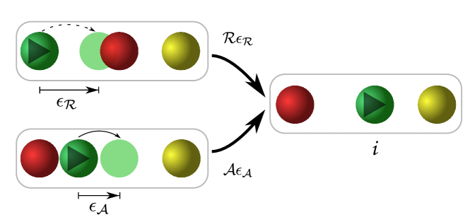
Figure 2: Flow of the forward swap Metropolis algorithm  into a configuration $(a,i)$ (the active sphere $i$ is shown in green). A rejected sphere move, by a displacement $\epsilon_{\mathcal{R}}$ (upper case), entails a swap and contributes $\mathcal{R}_{\epsilon_{\mathcal{R}}}$. An accepted sphere move, by a displacement $\epsilon_{\mathcal{A}}$ (lower case), contributes $\mathcal{A}_{\epsilon_{\mathcal{A}}}$. For any $\epsilon$, one of the flows equals one, and the other zero [$(\mathcal{R}_{\epsilon},\mathcal{A}_{\epsilon})\in\{(0,1),(1,0)\}$].

Irreversible Monte Carlo algorithms violate the detailed-balance condition of eq. (1) but instead satisfy the weaker global-balance condition

$$\sum_{b}\pi^{()}(b)p(b\to a)=\pi^{()}(a).$$ (2)

Together with the easily satisfiable aperiodicity and irreducibility conditions[6], the global-balance condition ensures that the steady-state solution corresponds to the probability $\pi^{()}$, but without necessarily cancelling the net flow $\pi^{()}(a)p(a\to b)-\pi^{()}(b)p(n\to a)$ between configurations $a$ and $b$ (cf eq. (1)). Here, we take up the forward Metropolis algorithm studied earlier, in a new variant that involves swaps. This allows us to arrive at an exact mixing result.

In the forward swap Metropolis algorithm, at each time step, a randomly chosen sphere $i$ attempts to move by a random displacement $\epsilon$ with a predefined sign (that for clarity, we take to be positive). If the move is rejected (that is, the displacement $\epsilon$ does not yield a valid hard-sphere configuration), the sphere swaps its label with the sphere responsible for the rejection (see the upper move in Fig. 2). Else, if the displacement $\epsilon$ is accepted, the sphere $i$ simply moves forward (see the lower move in Fig. 2). The total flow into a configuration $(a,i)$ (that is, the $N$-sphere configuration $a$ with the active sphere $i$) is:

$$\mathcal{F}(a,i)=\int_{0}^{\infty}\mathrm{d}\epsilon p(\epsilon)\underbrace{\left[\mathcal{A}_{\epsilon}(a,i)+\mathcal{R}_{\epsilon}(a,i)\right]}_{=1\ \text{(see Fig.~{}\ref{fig:MoveSwap})}}=1=\pi(a),$$ (3)

so that the algorithm satisfies global balance. The swap allows both the rejected and the accepted moves into the configuration $(a,i)$ to involve the sphere $i$ only. The forward swap Metropolis algorithm is equivalent (up to relabeling) to the forward Metropolis algorithm treated earlier if at each time step the active sphere $i$ is sampled randomly. The mixing time of this algorithm was conjectured to be $\mathcal{O}({N^{5/2}})$, based on numerical simulations[15]. This agrees with the proven mixing time scale of the totally asymmetric simple exclusion process (TASEP)[28].

Figure 3: Forward swap Metropolis algorithm, with configurations $\mathbf{x}_{t},\ldots,\mathbf{x}_{t+5}$. The active sphere is sampled randomly at each time step so that the swaps have no other action than to relabel the spheres.

The forward swap Metropolis algorithm satisfies global balance for any choice of the sphere $i$ and any step-size distribution $p(\epsilon)$. This implies that the active-sphere index $i$ need not be sampled randomly for the algorithm to remain valid. This distinguishes it from the forward Metropolis algorithm (without the swaps) treated in previous work[15]. In particular, the sphere $i$ can be active for several chains in a row. The algorithm, run with the following sequence of active spheres:

$$\dots,\underbrace{i,i,\dots,i,i}_{\text{chain $n$}},\underbrace{j,j,\dots,j,j}_{\text{chain $n+1$}},\underbrace{k,k,\dots,k,k}_{\text{chain $n+2$}},\dots,$$ (4)

is equivalent to the lifted forward Metropolis algorithm studied earlier[15], if the active spheres $i,j,k,\dots$ in eq. (4) are sampled randomly. The algorithm naturally satisfies the global balance condition, and again, each individual move attempts a displacement by a distance $\epsilon$ sampled from a given distribution $p(\epsilon)$ that vanishes for negative $\epsilon$, and the chain lengths (number of repetitions of $i,j,k,\dots$) $n,n+1,\dots$ are sampled from a distribution. Numerical simulations have lead to the conjecture that this algorithm mixes in $\mathcal{O}({N^{2}\log N})$ time steps[15].

ECMC is the continuous-time limit of the lifted forward Metropolis algorithm, with the simultaneous limits $\epsilon\to 0$ and $l\to\infty$, but $\left(\left\langle\epsilon\right\rangle l\right)\to\ell$, where the chain length $\ell$ on the scale $L_{\text{free}}$, is again sampled from a given probability distribution. In the point-particle representation of Fig. 1(b), one “event” chain of the ECMC algorithm simply moves the active particle $i$ from its initial position $x_{i}$ to $x_{i}+\ell$. It advances the time as $t\to t+\ell$, and increments the number of chains as $n\to n+1$. The number of eponymous “events” of ECMC (the number of changes of the active sphere) then grows approximately as $\sim(\ell/L_{\text{free}})N$. When $\ell\sim\text{unif}\left(0,L_{\text{free}}\right)$, this places particle $i$ at a random position on a ring. For this special uniform distribution of chain lengths, a perfect sample is clearly obtained once all particles were at least once picked as the active particle. This situation will now be analyzed in terms of the coupon-collector problem (see [33, 34]).

For the ECMC with $\ell\sim\text{unif}\left(0,L_{\text{free}}\right)$, the TVD can be expressed by the probability that at least one particle has never been picked as an active particle of a chain. Without restriction, we suppose that the initial configuration is the compact state $\mathbf{x}=\{0,0,\ldots,0\}$. We also measure time in the number of chains $n$ ($n$ translates into an MCMC time as $t(n)=\left\langle\ell\right\rangle n$ and is easily converted into the number of events). In eq. (LABEL:equ:SecondDefinitionTVD), the set $\mathcal{A}$ is

$$\mathcal{A}=\{\mathbf{x}\ |\ \exists\ i\ \text{with}\ x_{i}=0\}.$$ (5)

Also, clearly, $\pi^{(n)}(\mathcal{A})$ equals the probability that at least one particle has never been picked as an active particle of a chain, whereas $\pi^{()}(\mathcal{A})=0$, as it is a lower-dimensional subset of $\Omega$. From eqs (LABEL:equ:FirstDefinitionTVD) and (LABEL:equ:SecondDefinitionTVD), therefore (for $N\to\infty$):

$$\|\pi^{(n)}-\pi^{()}\|_{\text{TV}}\sim 1-\exp\left[-\exp\left(-\frac{n-N\log N}{N}\right)\right],$$ (6)

where we used the analytically known asymptotic tail probability for the coupon-collector problem[33] (see Fig. 4).

Rather than computing the difference between $\pi^{(n)}$ and $\pi^{()}$ at a fixed number $n$ of chains, one can simply run ECMC (with $\ell\sim\text{unif}\left(0,L_{\text{free}}\right)$) until the time at which chains with any of the $N$ particles as active ones have completed. The expected number of chains or, in the language of the coupon-collector problem, the expected value of $n_{1}$ to “collect the last coupon” is given by

$$\left\langle n_{1}\right\rangle=NH_{N}=N\log N+\gamma N+\frac{1}{2}+\mathcal{O}({1/N}),$$ (7)

where $H_{N}=\frac{1}{1}+\frac{1}{2}+\dots+\frac{1}{N}$ is the $N$th harmonic number and $\gamma=0.5772...$ is the Euler-Mascheroni constant. The distribution of this number of chains can be obtained from the tail distribution contained in eq. (6) (see Fig. 4). In both ways, we see that mixing takes place after $\mathcal{O}({N\log N})$ chains (corresponding to $\mathcal{O}({N^{2}\log N})$ events), confirming, for a special distribution of $\ell$, an earlier conjecture[15]. The discussed mixing behavior of ECMC can more generally be obtained for distributions $\ell\sim\text{unif}\left(c,c+L_{\text{free}}\right)$ with arbitrary (and even with negative) $c$. In our special case, choosing $c=-L_{\text{free}}/2$ would lead to the smallest number of individual events. In view of the practical applications of ECMC, it appears important to understand whether this dependence on the distribution of $\ell$ rather than on its mean value has some relevance for the simulation of discrete 1D models, and whether it survives in higher dimensions, and for continuous (non-hard-sphere) potentials.

We next consider more general distributions, namely the uniform distribution $\ell\sim\text{unif}\left(0,\lambda L_{\text{free}}\right)$, as well as the Gaussian distribution $\mathcal{N}(\mu,\sigma^{2})$, where $\mu$ is the mean value and $\sigma$ the standard deviation. Again, particles are effectively independent and we conjecture the mixing time (which can now never lead to perfect sampling) to be governed by the particle which has moved the least number, $m$, of times. This is equivalent to the $m$-coupon generalization of the coupon-collector problem[33], whose tail probability is given by:

$$P(n_{m})=\exp\left(-\Upsilon/(m-1)!$$ (8)

with

$$\Upsilon=\exp\left[-\frac{n_{m}-N\log N-(m-1)N\log\log N}{N}\right]$$ (9)

(see Fig. 4). This means that the number of chains to collect each of the $N$ coupons at least $m$ times only add an $N\log\log N$ correction to the general $N\log N$ scale of chains.

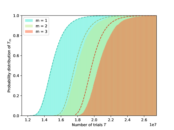
Figure 4: Cumulative probability of the coupon collector problem ($m=1$), and of the $m$-coupon collector problem for $m=2$ and $m=3$. Numerical simulations for $N=2^{20}$ particles are compared to the asymptotic tail probability of eq. (9).

To gain intuition, we now compute the TVD for the single-particle problem (for which $\ell\equiv\epsilon$). For simplicity, we set $L_{\text{free}}=1$ (measure the standard deviations in units of $L_{\text{free}}$). The TVD for chain lengths $\ell_{i}\sim\text{unif}\left(0,\lambda\right)$, as discussed, equals the one for $\ell_{i}\sim\text{unif}\left(-\lambda/2,\lambda/2\right)$. The sum of $m$ chains then follows the distribution:

$$p^{\text{unif}}_{m}(x)=\int_{-\infty}^{\infty}\mathrm{d}t\mathrm{e}^{-2\pi itx}\left[\frac{\sin\left(\pi\lambda t\right)}{\pi\lambda t}\right]^{m}$$ (10)

Using the Poisson summation formula and subtracting the equilibrium distribution $\pi^{()}=1$, we find:

$$\sum_{k=-\infty}^{\infty}p^{\text{unif}}_{m}(x+k)-1=\sum_{k\in\mathbb{N^{+}}}2\left[\frac{\sin\left(\pi k\lambda\right)}{\pi k\lambda}\right]^{m}\cos{\left(2\pi kx\right)}.$$

The total variation distance for chain lengths $\ell_{i}\sim\text{unif}\left(0,\lambda\right)$ thus satisfies:

$$\|\pi^{(m)}-\pi^{()}\|_{\text{TV}}\\ =\int_{0}^{1}dx\left|\sum_{k\in\mathbb{N^{+}}}\left[\frac{\sin\left(\pi k\lambda\right)}{\pi k\lambda}\right]^{m}\cos{\left(2\pi kx\right)}\right|\\ \sim\frac{2}{\pi}\left|\frac{\sin\left(\pi\lambda\right)}{\pi\lambda}\right|^{m}\ (\text{for}\quad m\to\infty).$$ (11)

The TVD trivially vanishes for integer $\lambda$ (see Fig. 5a). Its peaks decay as $\frac{2}{\pi}(\pi\lambda)^{-m}$.

For Gaussian-distributed chain lengths $\ell_{i}\sim\mathcal{N}(\mu,\sigma^{2})$, the sum of $m$ chains is distributed as:

$$\sum_{i=1}^{m}\ell_{i}\sim\mathcal{N}(m\mu,m\sigma^{2}).$$ (12)

With $\vartheta_{3}$ the Jacobi theta function, we now have

$$\sum_{k=-\infty}^{\infty}p^{\text{Gauss}}_{m}(x+k)-1=\vartheta_{3}\left[\pi(x+\mu),\exp\left(-2\pi^{2}m\sigma^{2}\right)\right]\\ =2\sum_{k=1}^{\infty}\exp\left(-2k^{2}\pi^{2}m\sigma^{2}\right)\cos\left[2k\pi(x+m\mu)\right].$$ (15)

The total variation distance for the distribution of eq. (12) satisfies:

$$\|\pi^{(m)}-\pi^{()}\|_{\text{TV}}\\ =\int_{0}^{1}dx\left|\sum_{k=1}^{\infty}\exp\left(-2k^{2}\pi^{2}m\sigma^{2}\right)\cos\left(2k\pi x\right)\right|\\ \sim\frac{2}{\pi}\exp\left(-2\pi^{2}m\sigma^{2}\right)\ (\text{for}\quad m\sigma^{2}\to\infty)$$ (19)

(see Fig. 5b).

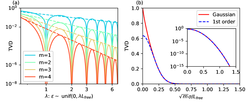
Figure 5: TVD for a single sphere on a ring with uniform and Gaussian distributions of $\ell\equiv\epsilon$. (a): TVD after $m$ displacements $\epsilon\sim\text{unif}\left(0,\lambda L_{\text{free}}\right)$. The TVD trivially vanishes for integer $\lambda$. Peaks decay as $\frac{2}{\pi}(\pi\lambda)^{-m}$ (for $m\to\infty$). (b): TVD for $m$ Gaussian displacements with standard deviation $\sigma$, compared with its first order approximation from the Jacobi $\vartheta$ function (see eq. (19)). The inset illustrates the good agreement of the approximation on a logarithmic scale.

Both for the uniform and the Gaussian distribution, the single-sphere TVD decreases exponentially with the number $m$ of displacements (which are equivalent to single-particle chains). We expect the same behavior for the $N$-sphere problem, where $m$ is now the number of chains for the $m$-coupon problem.

4 Sequential forward Metropolis, sequential ECMC

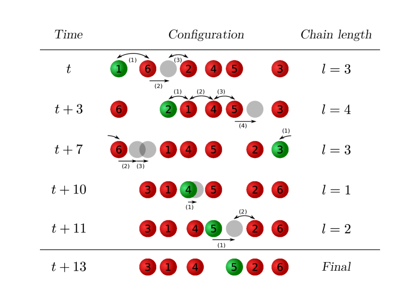
Figure 6: Sequential lifted forward Metropolis algorithm (with swaps). Configurations $\mathbf{x}_{t},\ldots,\mathbf{x}_{t+13}$ sampled through five chains with active sphere $1,2,\ldots,5$ are shown. Chain lengths are $l_{1}=3,\ldots,l_{5}=2$. Each sphere displacement $\epsilon_{t}>0$ is either accepted or, if rejected, it induces a swap, so that the same sphere remains active throughout a chain.

ECMC, with randomly sampled initial spheres and a standard deviation of the chain-length distribution $\sigma\sim L_{\text{free}}$, mixes in $\mathcal{O}({N^{2}\log N})$ events (corresponding to $\mathcal{O}({N\log N})$ chains). In the label-switching framework of ECMC, each chain consists in advancing the particle $i$ by a distance $\ell$ times, and both the ECMC and the forward-Metropolis versions are correct. Instead of sampling the active sphere for each chain, so that the coupon-collector aspect necessarily brings in the $\log N$ factor in the scaling of mixing times, we may also sequentially increment the active-sphere index for each chain (see Fig. 6):

$$\dots,\underbrace{i,\dots,i}_{\text{chain}\ i},\underbrace{i+1,\dots,i+1}_{\text{chain}\ i+1},\underbrace{i+2,\dots,i+2}_{\text{chain}\ i+2},\dots,$$ (20)

(where particle numbers are implied modulo $N$). Sequential ECMC, with a distribution $\ell_{i}\sim\text{unif}\left(0,L_{\text{free}}\right)$ produces an exact sample in $\mathcal{O}({N^{2}})$ events (corresponding to exactly $N$ chains).

Evidently, the analysis of eqs (11) and (19) can be applied to the sequential ECMC with distributions such as $\text{unif}\left(0,\lambda L_{\text{free}}\right)$ and, more generally, distributions with $\sigma\sim L_{\text{free}}$. After each “sweep” of chains, the TVD factorizes, and we expect mixing to take place after $\mathcal{O}({N})$ chains (corresponding to $\mathcal{O}({N^{2}})$ events).

ECMC is the limit of the lifted forward Metropolis algorithm, and the sequential ECMC the limit of the sequential lifted forward Metropolis algorithm for step sizes much smaller than the mean free space between spheres ($\left\langle\epsilon\right\rangle=L_{\text{free}}/(2N\alpha)$ with $\alpha\gg 1$). For a given discretization $2/\alpha$, and for small $N$, the sequential lifted forward algorithm mimics the $\mathcal{O}({N^{2}})$ mixing of the sequential ECMC, but for large $N$, it seems to cross over into $\mathcal{O}({N^{2}\log N})$ mixing (see Fig. 7a). $\mathcal{O}({N^{2}})$ mixing also emerges at fixed $N$ for large $\alpha$ (see Fig. 7b). (This is obtained using the heuristic mid-system variance $x_{i+N/2}-x_{i}$ for ordered $x_{i}$, see [15].) In contrast, the random lifted forward Metropolis algorithm shows $\mathcal{O}({N^{2}\log N})$ mixing (see Fig. 7c), as discussed earlier [15]. This scaling is little influenced by the discretization (see Fig. 7d). It thus appears that the $N\to\infty$ limit of the sequential lifted forward Metropolis algorithm does not commute with the small discretization limit $\alpha\to\infty$.

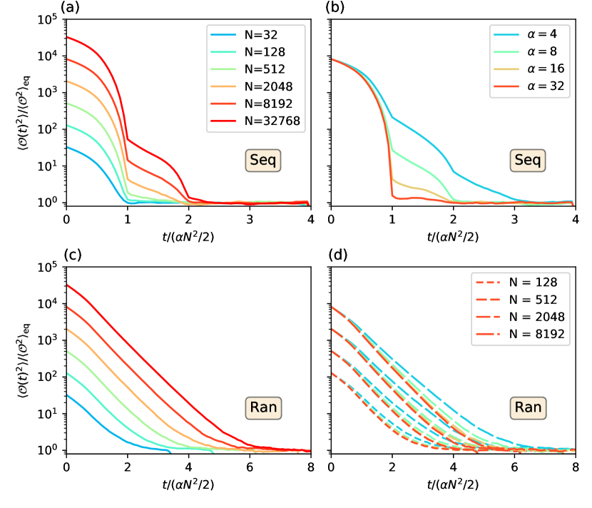
Figure 7: Crossover from the discrete lifted algorithm to ECMC, via the variance of the mid-system distance $x_{i+N/2}-x_{i}$ for ordered $x_{i}$, started from compact initial condition (see [15]). Discrete step size with $\epsilon\sim\text{unif}\left(0,L_{\text{free}}/N/\alpha\right)$, and chain length $l\sim\text{unif}\left\{\alpha,\alpha N\right\}$ (a): Sequential lifted Metropolis with constant $\alpha=10$ for different $N$: The cross-over from perfect sampling for small $N$ at a time scale $\mathcal{O}({N^{2}})$ towards $\mathcal{O}({N^{2}\log N})$ appears evident. (b): Sequential algorithm for $N=8192$, with increasing $\alpha$: $\mathcal{O}({N^{2}})$ mixing scale emerges for large $\alpha$. (c): Random lifted Metropolis with $\alpha=10$ for different $N$ (legend as in (a)): $\mathcal{O}({N^{2}\log N})$ mixing time scale (conjectured earlier[15]). (d): Random lifted forward Metropolis algorithm: Limited role of $\alpha$ (color code for $\alpha$ as in (b)).

5 Conclusions

In this paper we have proven that for 1D hard spheres, ECMC with a uniform distribution of chain length $\ell\sim[0,L_{\text{free}}]$, with $L_{\text{free}}=L-Nd$ realizes a perfect sample in $\mathcal{O}({N^{2}\log N})$ events that correspond to $\mathcal{O}({N\log N})$ chains. This confirms, in a special case, an earlier conjecture[15] for the mixing time of ECMC. For this case, we can compute the TVD but also indicate a stopping rule for a time (which depends on the particular realization of the Markov chain), after which the Markov chain is in equilibrium. We have also provided numerical evidence that the $N^{2}\log N$ mixing prevails for other distributions of $\ell$, namely for the uniform distribution $\text{unif}\left(0,\lambda L_{\text{free}}\right)$ and the Gaussian, and used the coupon-collector approximation to justify this approximation.

We have furthermore discussed a sequential ECMC which mixes in a time $\mathcal{O}({N^{2}})$. For this algorithm, “particle swaps” are essential. We have checked that the discrete version of this algorithm, namely the sequential lifted forward Metropolis algorithm crosses over, as the number $N$ of spheres is increased, to an $\mathcal{O}({N^{2}\log N})$ mixing behavior. In this formula, the origin of the logarithm is unclear, as it can no longer stem from the coupon collector. It would be of great interest for the fundamental understanding of irreversible MCMC algorithms to extend the results from ECMC to discrete versions, that is the lifted forward Metropolis algorithm and its sequential variant, as well as to the corresponding lattice models that may be easier to treat.

The lessons from our analysis of 1D hard-sphere systems are threefold. First, irreversible Markov chains can be proven to mix on shorter time scales than reversible algorithms. Second, the speed of ECMC depends on the whole distribution of the chain lengths $\ell$, but not on its mean value. Third, sequential-update algorithms (that remain valid in higher dimensions) can mix on faster time scales than random-update versions. It remains to be seen how these lessons carry over to more intricate models and to higher dimensions.

- [1] \NameMetropolis N., Rosenbluth A. W., Rosenbluth M. N., Teller A. H. Teller E. \REVIEWJ. Chem. Phys.2119531087.
- [2] \NameDevroye L. \BookNon-Uniform Random Variate Generation (Springer New York) 1986.
- [3] \NameKrauth W. \BookStatistical Mechanics: Algorithms and Computations (Oxford University Press) 2006.
- [4] \NameMartinelli F. \BookLectures on Glauber Dynamics for Discrete Spin Models in \BookLectures on Probability Theory and Statistics: Ecole d’Eté de Probabilités de Saint-Flour XXVII - 1997, edited by \NameBernard P. (Springer, Berlin, Heidelberg) 1999 pp. 93–191.
- [5] \NameLubetzky E. Sly A. \REVIEWComm. Math. Phys.3132012815.
- [6] \NameLevin D. A., Peres Y. Wilmer E. L. \BookMarkov Chains and Mixing Times (American Mathematical Society) 2008.
- [7] \NameDiaconis P. \REVIEWJ. Stat. Phys.1442011445.
- [8] \NameBerg B. A. \BookMarkov Chain Monte Carlo simulations and their statistical analysis: with web-based Fortran code (World Scientific) 2004.
- [9] \NameLandau D. Binder K. \BookA Guide to Monte Carlo Simulations in Statistical Physics (Cambridge University Press) 2013.
- [10] \NamePropp J. G. Wilson D. B. \REVIEWRandom Structures & Algorithms91996223.
- [11] \NameTuritsyn K. S., Chertkov M. Vucelja M. \REVIEWPhysica D2402011410.
- [12] \NameFernandes H. C. Weigel M. \REVIEWComput. Phys. Commun.18220111856.
- [13] \NameBernard E. P., Krauth W. Wilson D. B. \REVIEWPhys. Rev. E802009056704.
- [14] \NameMichel M., Kapfer S. C. Krauth W. \REVIEWJ. Chem. Phys.1402014054116.
- [15] \NameKapfer S. C. Krauth W. \REVIEWPhys. Rev. Lett.1192017240603.
- [16] \NameBernard E. P. Krauth W. \REVIEWPhys. Rev. Lett.1072011155704.
- [17] \NameLei Z. Krauth W. \REVIEWEPL (Europhysics Letters)121201810008.
- [18] \NameKampmann T. A., Boltz H.-H. Kierfeld J. \REVIEWJ. Chem. Phys.1432015044105.
- [19] \NameHarland J., Michel M., Kampmann T. A. Kierfeld J. \REVIEWEPL (Europhysics Letters)117201730001.
- [20] \NameFaulkner M. F., Qin L., Maggs A. C. Krauth W. \REVIEWarXiv 1804.057952018.
- [21] \NameKapfer S. C. Krauth W. \REVIEWPhys. Rev. E942016031302.
- [22] \NameDiaconis P., Holmes S. Neal R. M. \REVIEWAnnals of Applied Probability102000726.
- [23] \NameRandall D. Winkler P. \BookMixing Points on an Interval in proc. of \BookProceedings of the Seventh Workshop on Algorithm Engineering and Experiments and the Second Workshop on Analytic Algorithmics and Combinatorics, ALENEX /ANALCO 2005, Vancouver, BC, Canada, 22 January 2005 2005 pp. 218–221.
- [24] \NameRandall D. Winkler P. \BookMixing Points on a Circle Vol. 3624 of Lecture Notes in Computer Science (Springer, Berlin, Heidelberg) 2005 pp. 426–435.
- [25] \NameLacoin H. \REVIEWAnn Inst H Poincaré Probab Statist5320171402.
- [26] \NameGwa L.-H. Spohn H. \REVIEWPhys. Rev. Lett.681992725.
- [27] \NameChou T., Mallick K. Zia R. K. P. \REVIEWRep. Prog. Phys.742011116601.
- [28] \NameBaik J. Liu Z. \REVIEWJ. Stat. Phys.16520161051.
- [29] \NameHoover W. G. Ree F. H. \REVIEWJ. Chem. Phys.4919683609.
- [30] \NameAlder B. J. Wainwright T. E. \REVIEWPhys. Rev.1271962359.
- [31] \NameWilson D. B. \REVIEWRandom Structures & Algorithms16200085.
- [32] \NameKannan R., Mahoney M. W. Montenegro R. \BookRapid mixing of several Markov chains for a hard-core model in proc. of \Book14th annual ISAAC Lecture Notes in Computer Science (Springer, Berlin, Heidelberg) 2003 pp. 663–675.
- [33] \NameErdős P. Rényi A. \REVIEWMagyar Tud. Akad. Mat. Kutató Int. Közl.61961215–220.
- [34] \NameBlom G., Holst L. Sandell D. \BookProblems and Snapshots from the World of Probability (Springer New York) 1994.