Fitting flavour symmetries:
the case of two-zero neutrino mass textures

Abstract

We present a numeric method for the analysis of the fermion mass matrices predicted in flavour models. The method does not require any previous algebraic work, it offers a $\chi^{2}$ comparison test and an easy estimate of confidence intervals. It can also be used to study the stability of the results when the predictions are disturbed by small perturbations. We have applied the method to the case of two-zero neutrino mass textures using the latest available fits on neutrino oscillations, derived the available parameter space for each texture and compared them. Textures $A_{1}$ and $A_{2}$ seem favoured because they give a small $\chi^{2}$, allow for large regions in parameter space and give neutrino masses compatible with Cosmology limits. The other “allowed” textures remain allowed although with a very constrained parameter space, which, in some cases, could be in conflict with Cosmology. We have also revisited the “forbidden” textures and studied the stability of the results when the texture zeroes are not exact. Most of the forbidden textures remain forbidden, but textures $F_{1}$ and $F_{3}$ are particularly sensitive to small perturbations and could become allowed.

I Introduction

Understanding fermion masses and mixings is probably one of the most stubborn problems the particle physics community has nowadays: we have plenty of data about masses and mixings, which present clear patterns of hierarchies, yet we are unable to understand their origin and their values. The Standard Model (SM) just parametrizes them with complete generality and satisfying all requirements of renormalizable quantum field theories. The most popular theories beyond the SM (supersymmetry for instance) do not add much on the subject. The solution of this problem is probably linked to the origin of the spontaneous symmetry breaking mechanism in the SM or to the question on why there are only three generations of fermions. Until the complete solution is found one may adopt a more modest bottom-up approach and try to find patterns that relate the many parameters that characterize flavour. One of the simplest approaches in this direction has been to find texture zeroes in the mass matrices that are compatible with the data (see Wilczek:1977uh ; Fritzsch:1977za ; Ramond:1993kv for the quark/lepton sector and Frampton:2002yf for the neutrino sector). These texture zeroes are supposed to be enforced by a symmetry (see for instance Grimus:2004hf ; Dev:2011jc ) or be approximate statements dictated by the dynamics of a more complete theory (for instance in many radiative neutrino mass models Zee:1985id ; Babu:1988ki neutrino masses can be computed and are proportional to the charged lepton masses, in that case the elements proportional to $m_{e}$ are expected to be much smaller than the others, see for instance delAguila:2011gr ; delAguila:2012nu ; Alcaide:2017xoe ). Here we will discuss Majorana neutrino mass textures in the spirit of Frampton:2002yf in which one looks for zeroes of the neutrino mass matrix in a basis in which the charged lepton mass matrix is already diagonal (the analysis of the texture zeroes with arbitrary charged lepton and neutrino mass matrices is much more complicated for it can be shown that some textures are trivial in the sense that they can be obtained from general matrices just by changing the flavour basis Branco:2007nn ). In particular, two-zero textures are very interesting because they give four relations among the nine real parameters needed to describe the Majorana neutrino mass matrix, and these relations can be checked against available data. In ref. Frampton:2002yf it was shown that there are only seven two-zero textures which can accommodate data on neutrino masses and mixings (all three-zero textures were already excluded). These textures have been extensively studied in the past (see Guo:2002ei ; Dev:2006qe ; Fritzsch:2011qv ; Meloni:2012sx ; Kitabayashi:2015jdj ; Zhou:2015qua ; Singh:2016qcf for recent analyses).

In most of the works the relations among parameters have been derived analytically for the different textures. These relations have been used to scan the parameter space, letting the six parameters measured in neutrino oscillation experiments vary in their allowed $3\sigma$ regions and checking if the two-zero texture relations are satisfied. In general, correlations among oscillation parameters are neglected. This is a good approximation for most of them, but we now know the exact shape of the allowed region in the parameters $s_{23}^{2}$–$\delta$ ($s_{23}^{2}=\sin^{2}\theta_{23}$ is the $2-3$ mixing, and $\delta$ the Dirac phase in the neutrino mixing matrix) is quite asymmetric. This is in part due to the octant ambiguity in $s_{23}^{2}$ and the asymmetry in $\delta$ due to matter effects.

Here we will present an extremely simple method, completely numerical since the beginning, and will use previous results as a testbed for the method. The method, based on the minimization of a generalized $\chi^{2}$ function, which incorporates the constraints imposed by the textures, is now possible thanks to the fact that the NuFIT collaboration Esteban:2016qun ; nufitweb   has made publicly available the $\Delta\chi^{2}$ of their fits to neutrino oscillation data, and to the new Monte Carlo tools as MultiNest Feroz:2008xx ; Feroz:2013hea that will allow us a very robust and efficient scanning of the parameter space. The method incorporates naturally $s_{23}^{2}$–$\delta$ correlations, allows us to compute the available parameter space after the texture zeros have been imposed and provides a standard $\chi^{2}$ comparative test of how well the different textures can accommodate the experimental data . It also generalizes trivially to the case in which the zeroes are only approximate . All this without the need of any previous algebraic work to disentangle the relations among parameters.

Although we have concentrated in neutrino mass two-zero textures using the last oscillations data available (NuFIT 2018, release 3.2 nufitweb ), an aim of this work is to provide a general template to analyze numerically the different flavour models which give predictions for neutrino masses. Therefore, the methods developed here can be applied to other neutrino mass models and also to quark mass matrices with texture zeroes or other constraints.

Thus, in section II we fix the notation and briefly introduce the different two-zero neutrino mass matrix textures. In section III we present the method we use to analyze the textures while in section IV we study the available parameter space for all the allowed textures. In section V we discuss how the results change if the texture zeroes are only approximate and also review non-allowed textures when the zeroes are only approximate. Finally in section VI we collect the main conclusion of our analysis.

II The two-zero textures

Two-zero neutrino textures in the Frampton:2002yf approach are defined in the basis in which the charged lepton Yukawa matrices are diagonal and there are only three active neutrino characterized by a Majorana neutrino complex symmetric matrix . In this basis, the neutrino mass matrix can be reconstructed from the six neutrino oscillation parameters, $s_{12}^{2}$, $s_{23}^{2}$, $s_{13}^{2}$, $\Delta_{21}=m_{2}^{2}-m_{1}^{2}$, $\Delta_{31}=m_{3}^{2}-m_{1}^{2}$ and $\delta$, and three more parameters still unknown, the lightest neutrino mass $m_{\ell}$ (which is equal to $m_{1}$ in the normal ordering (NO) solution and $m_{3}$ in the inverted one (IO)) and two Majorana phases, $\alpha_{1}$ and $\alpha_{2}$:

$$M_{\nu}\equiv\begin{pmatrix}M_{ee}&M_{e\mu}&M_{e\tau}\\ M_{e\mu}&M_{\mu\mu}&M_{\mu\tau}\\ M_{e\tau}&M_{\mu\tau}&M_{\tau\tau}\end{pmatrix}=UD_{\nu}U^{T}\;,\quad{\rm with}\;\;D_{\nu}=\mathrm{diag}(m_{1},m_{2},m_{3})$$ (1)

where $U$ is the PMNS matrix and can be written as

$$U=\left(\begin{array}[]{ccc}c_{13}c_{12}&c_{13}s_{12}&s_{13}e^{-i\delta}\\ -c_{23}s_{12}-s_{23}s_{13}c_{12}e^{i\delta}&c_{23}c_{12}-s_{23}s_{13}s_{12}e^{i\delta}&s_{23}c_{13}\\ s_{23}s_{12}-c_{23}s_{13}c_{12}e^{i\delta}&-s_{23}c_{12}-c_{23}s_{13}s_{12}e^{i\delta}&c_{23}c_{13}\end{array}\right)\left(\begin{array}[]{ccc}e^{i\alpha_{1}/2}\\ &e^{i\alpha_{2}/2}\\ &&1\end{array}\right)\ ,$$ (8)

Two-zero textures impose that $(M_{\nu})_{ab}=0$ for two different elements. There are ${\displaystyle{\displaystyle\binom{6}{2}=15}}$ two-zero neutrino textures which were classified in ref. Frampton:2002yf in two groups; allowed

$$A_{1}:\,\begin{pmatrix}0&0&X\\ 0&X&X\\ X&X&X\end{pmatrix}\;,,\qquad A_{2}:\,\begin{pmatrix}0&X&0\\ X&X&X\\ 0&X&X\end{pmatrix}\;,$$ (9)

$$B_{1}:\,\begin{pmatrix}X&X&0\\ X&0&X\\ 0&X&X\end{pmatrix}\;,\qquad B_{2}:\,\begin{pmatrix}X&0&X\\ 0&X&X\\ X&X&0\end{pmatrix}\;,$$ (10)

$$B_{3}:\,\begin{pmatrix}X&0&X\\ 0&0&X\\ X&X&X\end{pmatrix}\;,\qquad B_{4}:\,\begin{pmatrix}X&X&0\\ X&X&X\\ 0&X&0\end{pmatrix}\;,$$ (11)

$$C:\,\begin{pmatrix}X&X&X\\ X&0&X\\ X&X&0\end{pmatrix}\;,$$ (12)

and 8 textures which were already forbidden by data at the time they were introduced:

$$D_{1}:\,\begin{pmatrix}X&X&X\\ X&0&0\\ X&0&X\end{pmatrix}\;,\qquad D_{2}:\,\begin{pmatrix}X&X&X\\ X&X&0\\ X&0&0\end{pmatrix}\;,$$ (13)

$$E_{1}:\,\begin{pmatrix}0&X&X\\ X&0&X\\ X&X&X\end{pmatrix}\;,\qquad E_{2}:\,\begin{pmatrix}0&X&X\\ X&X&X\\ X&X&0\end{pmatrix}\;,\qquad E_{3}:\,\begin{pmatrix}0&X&X\\ X&X&0\\ X&0&X\end{pmatrix}\;,$$ (14)

$$F_{1}:\,\begin{pmatrix}X&0&0\\ 0&X&X\\ 0&X&X\end{pmatrix}\;,\qquad F_{2}:\begin{pmatrix}X&0&X\\ 0&X&0\\ X&0&X\end{pmatrix}\;,\qquad F_{3}:\,\begin{pmatrix}X&X&0\\ X&X&0\\ 0&0&X\end{pmatrix}\;,$$ (15)

Following a standard notation, in eqs. (9–15) we represent the position of the two zeroes of the complex symmetric matrix in eq. (1). Two complex zeroes in the mass matrix give 4 relations among the 9 real parameters entering $M_{\nu}$. Depending on the texture, these relations will involve mainly the well known oscillation parameters or the unknown non-oscillation parameters $m_{\ell}$, $\alpha_{1}$ and $\alpha_{2}$ or a mixture of the two. For instance $A_{1}$ texture gives all the 3 unknown parameters in terms of the oscillation parameters, but in addition it gives a relation between $\delta$ and the rest of the oscillation parameters which can be tested against the experiment. On the other hand, $F_{1}$ gives several solutions, in one of them the masses are arbitrary but $s_{12}=0$ and $s_{13}=0$ and therefore it cannot accommodate neutrino oscillation data. Another solution, the only discussed usually in the literature, gives $\alpha_{1}=\alpha_{2}=-2\delta$ and arbitrary mixings, however, it requires exact degeneracy $m_{1}=m_{2}=m_{3}$, therefore $\Delta_{21}=0$ and $\Delta_{31}=0$, and it is also excluded.

It is important to remark that forbidden exact textures could become allowed if the zeroes are only approximate, we will discuss some examples in section V.

III The method

The NuFIT collaboration Esteban:2016qun ; nufitweb has fitted all neutrino data on oscillations and made available the obtained $\Delta\chi^{2}$ as a function of the six neutrino oscillations parameters $s_{12}^{2}$, $s_{23}^{2}$, $s_{13}^{2}$, $\Delta_{21}$, $\Delta_{31}$ and $\delta$ (well, they offer marginalized $\Delta\chi^{2}$ for each parameter individually and for all pairs of parameters). From their results one can conclude that, in general, the correlations are small except for the less known parameters $\delta$ and $s_{23}^{2}$ because the octant ambiguity. Therefore, from their data one can approximately reconstruct the complete $\Delta\chi^{2}$ as

$$\Delta\chi_{\nu f}^{2}\approx\Delta\chi^{2}(s_{23}^{2},\delta)+\Delta\chi^{2}(s_{13}^{2})+\Delta\chi^{2}(s_{12}^{2})+\Delta\chi^{2}(\Delta_{21})+\Delta\chi^{2}(\Delta_{31})-4\Delta\chi_{\mathrm{min}}^{2},$$ (16)

where the last term takes into account that the NuFIT collaboration normalizes each of the different projections so that $\Delta\chi_{\mathrm{min}}^{2}=4.14$ in the case of IO, therefore we have to subtract four times $\Delta\chi_{\mathrm{min}}^{2}$ to keep the same normalization. We have checked that using this $\Delta\chi_{\nu f}^{2}$ one can reproduce reasonably well all correlation plots presented in ref. Esteban:2016qun ; nufitweb .

One way to see if the constraints imposed by the textures are compatible with the data would be to vary all the oscillations parameters in their allowed range (at 1$\sigma$, $2\sigma$, …) and check if the correlation is satisfied. Then, one can predict also the non-oscillation parameters. This was done for instance in Singh:2016cbe ; Singh:2016qcf . However, by using this method one does not take into account the correlations of $\delta$ with $s_{23}^{2}$, which can be very important in some cases.

Here we will use a different method, which has some advantages. We will define a new $\chi^{2}$ that incorporates the constraints imposed by the texture zeros with Lagrange multipliers

$$\chi^{2}=\Delta\chi_{\nu f}^{2}+\frac{1}{\lambda_{1}^{2}}|(M_{\nu})_{ab}|^{2}+\frac{1}{\lambda_{2}^{2}}|(M_{\nu})_{cd}|^{2}\,.$$ (17)

For $\lambda_{1,2}\rightarrow+\infty$ one should recover the NuFIT results while for $\lambda_{1,2}\rightarrow+0$ the constraints are enforced maximally. The interpretation of $\lambda_{1}$ and $\lambda_{2}$ is also clear: the new terms only give an appreciable contribution to the $\chi^{2}$ when $|(M_{\nu})_{ab}|>\lambda_{1}$ ($|(M_{\nu})_{cd}|>\lambda_{2}$). Then, using this method we can also discuss approximate zeroes. Also, in particular for a numerical treatment, one cannot set directly $\lambda_{1,2}$ to zero. For our purposes, as the rest of the parameters in the neutrino mass matrix must be at least $1$ meV, it will be enough to take $\lambda_{1,2}\ll 1$ meV. To be definite, in our simulations we will take always $\lambda_{1}=\lambda_{2}=0.1$ meV and will check that the results do not change if we take smaller values of the $\lambda$’s. Note that eq. (17) has the standard $\chi^{2}$ interpretation of a measured Re$\{(M_{\nu})_{ab}\}$,Im$\{(M_{\nu})_{ab}\},=0\pm\lambda_{1}$ and similarly for $(M_{\nu})_{cd}$.

The method has another advantage because we can compute the $\chi^{2}$ at the minimum. This value will give us an indication of how well the different textures are able to fit the data.

IV Analysis of the allowed textures

Following the method discussed above, we will analyze the different allowed textures. Since $s_{12}^{2}$, $s_{13}^{2}$, $\Delta_{21}$, $\Delta_{31}$ are well known from oscillation data, only textures that can accommodate their values will be allowed. $\delta$ and $s_{23}^{2}$ are less known and there is more freedom to accommodate their values. Thus it makes sense to represent the constraints imposed by the different textures in the plane $s_{23}^{2}$–$\delta$. For that purpose we perform a simulation varying $s_{12}^{2}$, $s_{13}^{2}$, $\Delta_{21}$, $\Delta_{31}$ in their allowed $3\sigma$ ranges and find the region compatible with the different textures in the $s_{23}^{2}$–$\delta$ plane superposed to the NuFIT results (this is shown, for instance on the left panel of figure 1). This gives a clear idea of the expected allowed regions when the texture constraints are imposed to the NuFIT data according to eq. (17). It is important to remark that while the constraints imposed by all the textures only depend on $\cos\delta$, and therefore are symmetric with respect $\delta=180^{\circ}$, the global fit to neutrino oscillation data is not, and this strongly constraints the overlap regions.

The result of the complete fit is shown on the right panels ($s_{23}^{2}$–$\delta$ allowed region, and the predictions for the non-oscillation parameters $m_{\ell},\alpha_{1},\alpha_{2}$ against $\delta$). In all cases contours correspond to two-dimensional 68.27% 95.45% 99.73% C.L. regions computed by minimization of the $\chi^{2}$ function in eq. (17) for a fixed pair or parameters with respect to the rest of parameters and then requiring $\chi^{2}-\chi_{\mathrm{min}}^{2}<2.30,6.18,11.83$. For a more efficient sampling of the parameter space we use a nested sampling algorithm (MultiNest Feroz:2008xx ; Feroz:2013hea ) and we do an explicit $\chi^{2}$ minimization on the Markov Chain points. As discussed above, we took $\lambda_{1}=\lambda_{2}=0.1$ meV and checked that, in the case of the allowed textures, the results do not change if we take $\lambda_{1}=\lambda_{2}=0.05$ meV. For $m_{\ell}$ we take values in the range $0$–$1000$ meV.

We have repeated this procedure for all the allowed textures. In section V we will discuss, in some cases, how the constraints are relaxed if the textures are only approximate by taking $\lambda_{1}=\lambda_{2}=5$ meV and also how forbidden textures can become allowed if texture zeroes are only approximate, by taking $\lambda_{1}=\lambda_{2}=1$ meV.

IV.1 A1 and A2 textures (only NO)

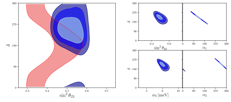
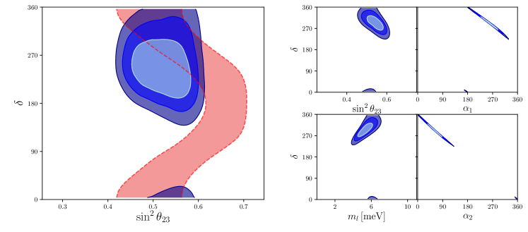
Figure 1: On the left of the panels we present the NuFIT results Esteban:2016qun ; nufitweb , in the $s_{23}^{2}$–$\delta$ plane, for the global fit to neutrino data (blue-gray coloured contours correspond to 68.27% 95.45% 99.73% C.L. regions ) as compared with the prediction of the textures, in red, obtained when the rest of the oscillation parameters are varied in 3$\sigma$. On the right we present the new fit to the data, as discussed in the text, when the constraints from the textures are imposed. The upper panel is for the $A_{1}$ texture and the lower one for the $A_{2}$ texture, which are only allowed in the NO case.

Both $A_{1}$ and $A_{2}$ textures require $(M_{\nu})_{ee}=0$ which is exactly the matrix element that controls the neutrinoless double beta decay rate, $m_{\beta\beta}=(M_{\nu})_{ee}$. It is well known the correlation between $m_{\beta\beta}$ and $m_{\ell}$ and the fact that in the IO case $m_{\beta\beta}$ is bounded from below, $m_{\beta\text{$\beta$}}\gtrsim 10\,$meV Bilenky:1999wz ; Vissani:1999tu , therefore, $A_{1}$ and $A_{2}$ textures are only allowed in the NO case.

The left panels of figure 1 show clearly that in the case of these two textures there are large regions of overlap between the NuFIT results and the constraint imposed by the textures with $A_{1}$ giving some preference for slightly smaller values of $\delta$ while $A_{2}$ prefers larger values.

On the right panels we present the constrained fit, eq. (17). The plane $s_{23}^{2}$–$\delta$ obviously gives the overlap regions shown on the left panels. In the rest of the plots we present the predictions for the non-oscillations parameters, $m_{\ell}$, $\alpha_{1}$ and $\alpha_{2}$ against $\delta$, which clearly show the strong correlation between the Majorana phases $\alpha_{1},\alpha_{2}$ and $\delta$ and the fact that in these two textures the lightest neutrino mass $m_{\ell}$ is predicted to be in a region around $5$ meV.

IV.2 B Textures

Textures of type $B$ are all very similar and, taking into account the ordering convention, we have eight of them. Basically they all predict $\delta\sim 270^{\circ}$ (or $\delta\sim 90^{\circ}$ which is strongly disfavoured by present fits), and $\alpha_{1}\sim\alpha_{2}\sim 180^{\circ}$. This is a consequence of the small value of $s_{13}^{2}$. They also give a lower bound on the lightest neutrino mass, $m_{\ell}$, of the order of $40$–$50$ meV. Thus, we present in figure 2 complete results only for texture $B_{1}$, in both NO and IO cases.

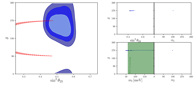
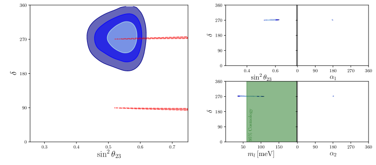
Figure 2: Same as figure 1 for the $B_{1}$ texture. Upper panels for NO and lower ones for IO . In the $\delta$–$m_{\ell}$ plot we also present, for comparison, the bound on the lightest neutrino mass obtained from Cosmology (we use $m_{\ell}<60$ meV Vagnozzi:2017ovm ).

On the left panels of figure 2 we see the constraints imposed by the $B_{1}$ texture for both the NO (above) and IO (below) superimposed to the NuFIT contour plots in the plane $\delta$-$s_{23}^{2}$. In the NO case $\delta$ is slightly below $270^{\circ}$ and $s_{23}^{2}<0.5$ while in the NO it is just the opposite ($\delta$ is slightly above $270^{\circ}$ and $s_{23}^{2}>0.5$). Since central values of NuFIT are slightly moved to higher values of $s_{23}^{2}$ in the case of IO, in this case it seems there is a larger overlap region. Notice that, as explained at the beginning of the section, to draw contours we always use contours of $\chi-\chi_{\mathrm{min}}$ and, therefore, these contours do not take into account that IO has a much larger value of $\chi^{2}$ ($4.14$ relative to NO).

On the right panels we present, as in figure 1, the results of the complete fit. The plots of $\delta$–$s_{23}^{2}$ just give the tiny overlap region for $\delta\sim 270^{\circ}$ and values of $s_{23}^{2}<0.5$ in the NO case or $s_{23}^{2}>0.5$ in the IO one. The $\alpha_{1},\alpha_{2}$ plots show they are basically fixed to $\alpha_{1}\sim\alpha_{2}=180^{\circ}$. The plot of $\delta$ versus $m_{\ell}$ is more interesting because it clearly shows that $m_{\ell}$ is bounded from below and can be rather large. For comparison we also give, in green, the band forbidden by Cosmology (we take $m_{\text{$\ell$}}\leq(m_{1}+m_{2}+m_{3})/3\lesssim$ $60\,\mathrm{meV}$, ref. Vagnozzi:2017ovm , which includes data from CMB and baryonic acoustic oscillations).

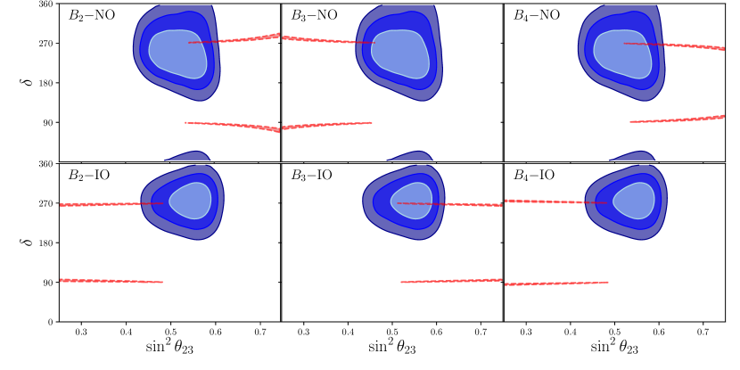
Figure 3: Same as the left panels of figure 2 for the $B_{2}$,$B_{3}$ and $B_{4}$ textures. Above for in NO and below for IO.

For the rest of $B$ textures we present in figure 3 the region allowed by the textures on top of the NuFIT results in the plane $s_{23}^{2}$–$\delta$. We can see the small differences between the different textures, $B_{1}$-NO,$B_{3}$-NO,$B_{2}$-IO,$B_{4}$-IO require $s_{23}^{2}<0.5$ while $B_{1}$-IO,$B_{3}$-IO,$B_{2}$-NO,$B_{4}$-NO require $s_{23}^{2}>0.5$. On the other hand $B_{1}$-NO,$B_{4}$-NO,$B_{2}$-IO,$B_{3}$-IO give $\delta$ values a bit below $270^{\circ}$ while $B_{1}$-IO,$B_{4}$-IO,$B_{2}$-NO,$B_{3}$-NO give $\delta$ a bit above $270^{\circ}$. The exact bands allowed at the $3\sigma$ level, together with the limits on the masses, are presented in table 1.

IV.3 C Texture

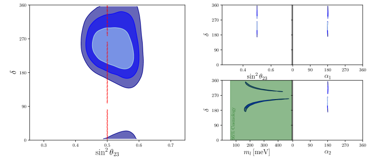
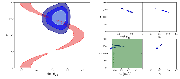
Figure 4: Same as figure 2 for the $C$ texture. In the upper panels for NO and the lower ones for IO.

Texture $C$, represented in figure 4, is probably the most peculiar of the textures since it divides the space of parameters in two disjoint regions according to the exact value of $\delta$ (this is clearly seen in the $\delta$–$m_{\ell}$ plot) .

In the case of NO it predicts $s_{23}^{2}\simeq 0.5$ with a high degree of precision (see for instance Grimus:2004az ) and forbids a small region around $\delta\sim 270^{\circ}$ (well, it requires very large values of $m_{\ell}$ to reach it). Since the last NuFIT results seem to favour values around $s_{23}^{2}=0.5$, as we will see in table 1, this texture gives one of the lowest values of the $\chi^{2}$, but this is at the cost of very large values of $m_{\ell}$, which, as shown in the $\delta$–$m_{\ell}$ plot, can be in conflict with Cosmology data. For the Majorana phases it gives $\alpha_{1}\sim\alpha_{2}\sim 180^{\circ}$ (see table 1 for the exact values).

The IO case is even more peculiar. It forbids small regions around $\delta=270^{\circ}$ and $s_{23}^{2}$ around $0.5$, and this is also translated into the possible values of $\alpha_{1}$ and $\alpha_{2}$. On the other hand, even though it also gives a lower bound on $m_{\ell}$, there is still some space to make it compatible with Cosmology.

IV.4 Best fit parameters

In table 1 we give the $3\sigma$ bands for the relevant parameters ($\Delta_{21}$, $\Delta_{31}$, $s_{12}$, $s_{13}$ are within the standard oscillation fit ranges) in the different allowed textures in both the NO and IO cases. We also present allowed bands for the lightest neutrino mass $m_{\text{$\ell$}}$, the Cosmology mass $m_{\mathrm{cos}}=m_{1}+m_{2}+m_{3}$ and the effective mass relevant for neutrinoless double beta decay $m_{\beta\beta}=|(M_{\nu})_{ee}|$. We also give the $\chi^{2}$ on the best fit parameters. Finally, to see the impact of the Cosmology bound, $m_{\ell}<60\,$meV, in the last column we also present the $\chi^{2}$ values obtained when $m_{\ell}<60\,$meV is imposed. Following the NuFIT collaboration, in the in the IO case we have included the value of the minimum, $4.14$, relative to the absolute minimum of NuFIT which happens for NO. However to compute the 3$\sigma$ bands we take, as usual, $\chi-\chi_{\mathrm{min}}=9$.

All textures considered, give $\chi^{2}$ values around 1 ($B_{2,4}$–IO which give slightly larger values). This is really interesting since, as discussed in the introduction, two-zero neutrino textures depend on only five real parameter from the six oscillation parameters.

On the other hand, looking at figs. 2–4 one can see that in the $s_{23}^{2}-\delta$ plane the constraints for $B^{\prime}s$ and $C$–NO are basically lines, so the amount of parameter space is very small. This can be measured using a Bayesian estimator, like the Bayes factor, but to compute it is technically complicated and has also its own conceptual problems because the comparison depends strongly on the volume of the priors and their parametrization, thus in this paper we decided to present only the $\chi^{2}$ values at the minimum.

	$m_{\ell}$	$m_{\mathrm{cos}}$	$m_{\beta\beta}$	$s_{23}^{2}$	$\delta$	$\alpha_{1}$	$\alpha_{2}$	$\chi^{2}$	$\chi_{m_{\ell}<60}^{2}$
$A_{1}$–NO	4.2–7.8	64-70	0–0.3	0.42–0.59	154–290	56–210	256–383	0.8	0.8
$A_{2}$–NO	3.4–7.1	62-69	0–0.3	0.45–0.62	217–369	169–334	-8–139	1.9	1.9
$B_{1}$–NO	>47	>170	50–245	0.42–0.50	267–270	180–187	177–180	0.7	4
$B_{1}$–IO	>37	>165	62–195	0.50–0.62	269–271	175-180	180–182	4.2	4.2
$B_{2}$–NO	>39	>147	41–202	0.50–0.61	270–274	170–180	180–184	0.7	1.5
$B_{2}$–IO	>48	>205	74–315	0.43–0.50	269–271	180–183	179–180	6.2	12
$B_{3}$–NO	>50	>179	53–249	0.42–0.50	270–273	176–180	180–182	0.7	5
$B_{3}$–IO	>40	>172	64–266	0.50–0.62	268–271	180–186	177-180	4.2	4.4
$B_{4}$ –NO	>41	>153	43–206	0.50–0.61	266–270	180–186	178–180	0.7	1.7
$B_{4}$–IO	>56	>212	76–334	0.43–0.50	269–271	176–180	180–182	6.2	13
$C$–NO	>159	>484	>151	0.50	175–262	178–180	178-180	0.2	>1000
	>167				278–346	180–182	180-182	1.1	>1000
$C$–IO	>35	>155	>34	0.51–0.61	231–269	186–281	151–178	4.8	5.1
	>67			0.44–0.49	273–289	120–168	185–202	6.7	13

Table 1: 99.73% C.L. results for the fits of the different textures. All masses are given in meV and all angles in degrees taken in the range $[0,360^{\circ}]$, except in some cases in which to avoid disjoint bands we have enlarged the region slightly below $0^{\circ}$ or above $360^{\circ}$. IO $\chi^{2}$ already include the $4.1$4 relative to NO obtained by the NuFIT collaboration but it is subtracted to compute the bands. We present also the $\chi^{2}$ values obtained when the Cosmology bound $m_{\ell}<60$ meV is imposed.

V Approximate texture zeroes

Above we have considered only allowed textures in the limit in which the texture zeroes are exact. In specific models the texture zeros come from symmetries which are slightly broken or are consequences of the dynamics (zeroes could arise only at some order of perturbation theory or be proportional to some small couplings). Moreover, one expects, that in some cases, radiative corrections will fill the texture zeroes with small quantities Hagedorn:2004ba . Then, it makes sense to ask how stable are the conclusions of our analysis against small perturbations. On the other hand, it is possible that textures that were considered excluded, if they are exact, become allowed if the zeroes are only approximate. The method proposed in this paper makes it trivial to discuss these problems.

To answer the first question we have considered the texture $B_{1}$–NO and studied how the parameter space changes when we move from $\lambda=0.1$ meV to $\lambda=5$ meV. This is a typical example with a very constrained parameter space ($\delta$, $\alpha_{1}$ and $\alpha_{2}$ are basically fixed). In figure 5 we compare the allowed parameter space in these two cases and see that when the texture zeroes are not exact the available parameter space increase enormously but still the main predictions of the texture remain.

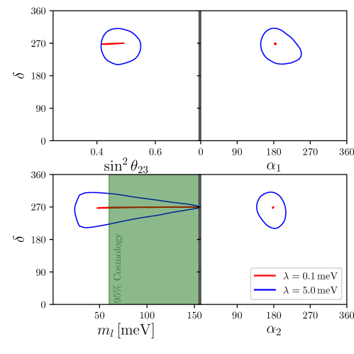
Figure 5: Allowed $3\sigma$ regions in the case of the $B_{1}$–NO texture when the texture zeroes are only approximate.

By using our method we could easily check quantitatively at which level the forbidden textures are excluded and how stable is this exclusion when the zeroes are not exact. Thus, we first minimized the $\chi^{2}$ in eq. (17) for $\lambda=0.1$ meV. We found that all textures, except $F$-type textures, give very large $\chi^{2}$ (larger than 50 for all of them and in some cases, $D$–NO, over $1000$). However, $F$-textures, give somehow lower values, and in particular $F_{1}$–$NO$ gives a fit with $\chi^{2}$ below $10$. These results are even more clear when we increase $\lambda$ from $0.1$ meV to $1$ meV, in which case $\chi^{2}$ as low as $0.5$ can be obtained ($F_{1}$–NO). while the rest of the forbidden textures still give a large $\chi^{2}$. To understand this result it is useful to see why exact $F$-textures are forbidden. Take the case of $F_{1}$ for instance, its mass matrix has two zeroes at the elements $(M_{\nu})_{12}$ and $(M_{\nu})_{13}$ and it is block-diagonal with $(M_{\nu})_{23}$ as the only non-trivial non-diagonal element. Then, one would conclude that $s_{12}=s_{13}=0$, which, of course, cannot accommodate neutrino oscillation data. However, this is not the only solution since, by taking the parametrization in eqs. (1–8), one can easily see that if $m_{1}=m_{2}=m_{3}$ there are also solutions with arbitrary mixings (see for instance Guo:2002ei ). This solution also implies that $\alpha_{1}=\alpha_{2}=-2\delta$ (or $\alpha_{1}=\alpha_{2}=2k\pi-2\delta$ $k=\pm 1,\pm 2,\cdots$). However, if masses are degenerate, $\Delta_{21}=\Delta_{31}=0$, and oscillation data cannot be accommodated either. In the method we are proposing all possible solutions are included automatically. Thus, in figure 6 we present results, in the case of $F_{1}$–NO, for $\lambda=0.1$ meV and $\lambda=1$ meV. All the oscillation parameters, including $\Delta_{31}$ and $\Delta_{21}$, can be adjusted easily in the two cases although for $\lambda=0.1$ meV $\chi^{2}$ is somehow larger but still below $9$. Moreover, to fit the data, large values of $m_{\ell}$ are required (see figure 6). If we take $\lambda=1$ meV the fit is much improved ($\chi^{2}$ below 1) and allows for much smaller values of $m_{\ell}$.

One interesting point is that the correlation between phases $\alpha_{1}=\alpha_{2}=-2\delta$, remains in spite of the non-exact texture zeros. This result can be understood by using standard degenerate perturbation theory: if the exact texture produces a degenerate spectrum and we introduce a small perturbation, it will shift the eigenvalues by a small quantity but the mixings, given by the eigenvectors which diagonalize the perturbation, will not be suppressed and can be as large as needed to fit the data. In the case of $F_{1}$–NO, for $M_{12,13}\ll m_{3}$ one typically finds

$$\Delta_{31}\propto\frac{1}{s_{13}}m_{3}|M_{12,13}|\;,\quad\Delta_{21}\propto m_{3}|M_{12,13}|$$

with coefficients which depend on $s_{12}$ and $s_{23}$. This shows a natural enhancement of $\Delta_{31}$ with respect to $\Delta_{21}$ due to the smallness of $s_{13}$. Moreover, since $\Delta_{31,21}$ are fixed by oscillations, and we are requiring $|M_{12,13}|<\lambda$, it is clear that, in general, smaller $\lambda$’s will require larger $m_{3}$ to fit the data, as clearly seen in figure 6. On the other hand, for the phases we have

$$e^{i(\alpha_{1}+2\delta)}\approx e^{i(\alpha_{2}+2\delta)}\approx 1+\mathcal{O}\left(\frac{M_{12,13}}{m_{3}}\right)$$

which explains the strong correlation of the Majorana phases with $\delta$ even when the texture is only approximate.

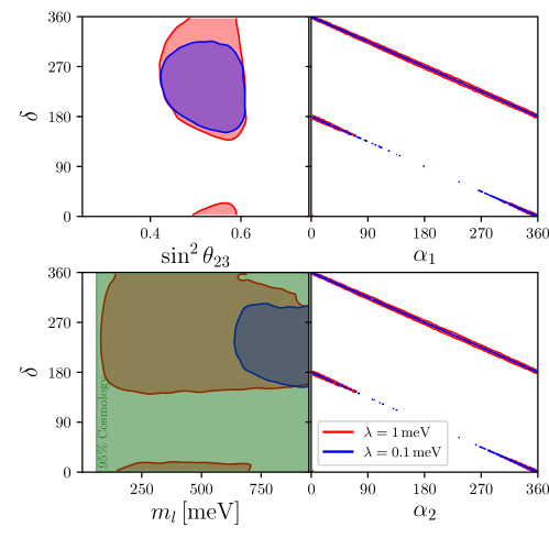
Figure 6: Allowed $3\sigma$ regions in the case of the “excluded” $F_{1}$–NO texture when the texture zeroes are only approximate.

VI Conclusions

We have introduced a new method, based on a $\chi^{2}$ analysis with constraints, to analyze numerically possible relations among the elements of the fermion mass matrices. As an example, we have applied it to the case of two-zero neutrino textures. The method has allowed us to disentangle the available parameter space, give correlation plots among parameters and confidence level bands without any algebraic work. We have also compared the different textures according the minimum $\chi^{2}$ they can give.

In the case of the known “allowed” textures, $A,B,C$ we have seen that, although in some cases $B$ and $C$ textures offer a fit with smaller values of $\chi^{2}$, $A$ textures are favoured with respect the rest of the allowed textures because:

-They have a larger parameter space: the highly restricted values of $\delta$ in the other textures, especially $B$ textures, will make it difficult to accommodate them if the oscillation data becomes more precise. In fact, already now textures $B_{2}$–IO and $B_{4}$–IO have no overlapping region at the 1$\sigma$ level with the last NuFIT results, which is manifested in a $\chi^{2}$ above $6$ (this already takes into account the IO $\chi^{2}$ minimum value of 4.14 relative to NO).

-All textures, except $A$–type textures, require large values of the lightest neutrino mass, $m_{\ell}\gtrsim 40$ meV, in particular $m_{\ell}\gtrsim 160$ meV in the $C$-NO texture. This can be in tension with Cosmology, which at present requires $m_{\ell}<60\,$meV. But, of course, there could be some, still unknown mechanism, that could make Cosmology data compatible with larger neutrino masses.

On the other hand, neutrinoless double beta decay experiments will provide another test of the textures. If it is found in the next round of experiments $A_{1}$ and $A_{2}$ textures, at least if they are exact, will be excluded since they require $m_{\beta\beta}=0$.

We have also discussed approximate texture zeros. We found that in the case of the allowed textures the general conclusions are not changed if the zero-matrix elements are below $1$ meV, although in the case of textures $B$, which have a strongly constrained parameter space, it is enlarged if the zeros are just $5$ meV. More importantly, we have also analyzed the case of forbidden textures by taking matrix elements below $1$ meV. In general, all forbidden textures remain forbidden (they give values of $\chi^{2}$ above $50$). However, textures of type $F$, could become allowed with $\chi^{2}$ which are below $1$, in particular, in the case of $F_{1}$–NO and $F_{3}$-NO.

Finally we have shown that the numeric method proposed in this paper is a good complement of the analytic studies to study the relations between Yukawa couplings/mass matrices imposed by symmetries or the flavour structure of the theory. The method incorporates naturally correlations among measured parameters, allows us to compute the available parameter space and provides a standard $\chi^{2}$ comparative test of how well the different models can accommodate the experimental data. It also generalizes trivially to the case in which the relations among parameters are only approximate.

- (1) F. Wilczek and A. Zee, Discrete Flavor Symmetries and a Formula for the Cabibbo Angle, Phys. Lett. B70 (1977) 418.
- (2) H. Fritzsch, Calculating the Cabibbo Angle, Phys. Lett. B70 (1977) 436–440.
- (3) P. Ramond, R. G. Roberts and G. G. Ross, Stitching the Yukawa quilt, Nucl. Phys. B406 (1993) 19–42, [hep-ph/9303320].
- (4) P. H. Frampton, S. L. Glashow and D. Marfatia, Zeroes of the neutrino mass matrix, Phys. Lett. B536 (2002) 79–82, [hep-ph/0201008].
- (5) W. Grimus, A. S. Joshipura, L. Lavoura and M. Tanimoto, Symmetry realization of texture zeros, Eur. Phys. J. C36 (2004) 227–232, [hep-ph/0405016].
- (6) S. Dev, S. Gupta and R. R. Gautam, Zero Textures of the Neutrino Mass Matrix from Cyclic Family Symmetry, Phys. Lett. B701 (2011) 605–608, [1106.3451].
- (7) A. Zee, Quantum Numbers of Majorana Neutrino Masses, Nucl. Phys. B264 (1986) 99–110.
- (8) K. S. Babu, Model of ’Calculable’ Majorana Neutrino Masses, Phys. Lett. B203 (1988) 132–136.
- (9) F. del Aguila, A. Aparici, S. Bhattacharya, A. Santamaria and J. Wudka, A realistic model of neutrino masses with a large neutrinoless double beta decay rate, JHEP 05 (2012) 133, [1111.6960].
- (10) F. del Aguila, A. Aparici, S. Bhattacharya, A. Santamaria and J. Wudka, Effective Lagrangian approach to neutrinoless double beta decay and neutrino masses, JHEP 06 (2012) 146, [1204.5986].
- (11) J. Alcaide, D. Das and A. Santamaria, A model of neutrino mass and dark matter with large neutrinoless double beta decay, JHEP 04 (2017) 049, [1701.01402].
- (12) G. C. Branco, D. Emmanuel-Costa, R. Gonzalez Felipe and H. Serodio, Weak Basis Transformations and Texture Zeros in the Leptonic Sector, Phys. Lett. B670 (2009) 340–349, [0711.1613].
- (13) W.-l. Guo and Z.-z. Xing, Implications of the KamLAND measurement on the lepton flavor mixing matrix and the neutrino mass matrix, Phys. Rev. D67 (2003) 053002, [hep-ph/0212142].
- (14) S. Dev, S. Kumar, S. Verma and S. Gupta, Phenomenology of two-texture zero neutrino mass matrices, Phys. Rev. D76 (2007) 013002, [hep-ph/0612102].
- (15) H. Fritzsch, Z.-z. Xing and S. Zhou, Two-zero Textures of the Majorana Neutrino Mass Matrix and Current Experimental Tests, JHEP 09 (2011) 083, [1108.4534].
- (16) D. Meloni and G. Blankenburg, Fine-tuning and naturalness issues in the two-zero neutrino mass textures, Nucl. Phys. B867 (2013) 749–762, [1204.2706].
- (17) T. Kitabayashi and M. YasuÚ, Formulas for flavor neutrino masses and their application to texture two zeros, Phys. Rev. D93 (2016) 053012, [1512.00913].
- (18) S. Zhou, Update on two-zero textures of the Majorana neutrino mass matrix in light of recent T2K, Super-Kamiokande and NOA results, Chin. Phys. C40 (2016) 033102, [1509.05300].
- (19) M. Singh, G. Ahuja and M. Gupta, Revisiting the texture zero neutrino mass matrices, PTEP 2016 (2016) 123B08, [1603.08083].
- (20) I. Esteban, M. C. Gonzalez-Garcia, M. Maltoni, I. Martinez-Soler and T. Schwetz, Updated fit to three neutrino mixing: exploring the accelerator-reactor complementarity, JHEP 01 (2017) 087, [1611.01514].
- (21) I. Esteban, M. C. Gonzalez-Garcia, M. Maltoni, I. Martinez-Soler and T. Schwetz, NuFIT 3.2 (2018), www.nu-fit.org., .
- (22) P. F. de Salas, D. V. Forero, C. A. Ternes, M. Tortola and J. W. F. Valle, Status of neutrino oscillations 2018: first hint for normal mass ordering and improved CP sensitivity, 1708.01186.
- (23) F. Capozzi, E. Lisi, A. Marrone and A. Palazzo, Current unknowns in the three neutrino framework, 1804.09678.
- (24) F. Feroz, M. P. Hobson and M. Bridges, MultiNest: an efficient and robust Bayesian inference tool for cosmology and particle physics, Mon. Not. Roy. Astron. Soc. 398 (2009) 1601–1614, [0809.3437].
- (25) F. Feroz, M. P. Hobson, E. Cameron and A. N. Pettitt, Importance Nested Sampling and the MultiNest Algorithm, 1306.2144.
- (26) C. Hagedorn, J. Kersten and M. Lindner, Stability of texture zeros under radiative corrections in see-saw models, Phys. Lett. B597 (2004) 63–72, [hep-ph/0406103].
- (27) W. Krolikowski, Fermion texture and sterile neutrinos, Acta Phys. Polon. B30 (1999) 2631–2669, [hep-ph/9903209].
- (28) Y. Zhang, Majorana neutrino mass matrices with three texture zeros and the sterile neutrino, Phys. Rev. D87 (2013) 053020, [1301.7302].
- (29) N. Nath, M. Ghosh and S. Gupta, Understanding the masses and mixings of one-zero textures in 3 + 1 scenario, Int. J. Mod. Phys. A31 (2016) 1650132, [1512.00635].
- (30) L. Lavoura, Zeros of the inverted neutrino mass matrix, Phys. Lett. B609 (2005) 317–322, [hep-ph/0411232].
- (31) G. C. Branco, R. Gonzalez Felipe, F. R. Joaquim and T. Yanagida, Removing ambiguities in the neutrino mass matrix, Phys. Lett. B562 (2003) 265–272, [hep-ph/0212341].
- (32) X.-G. He and A. Zee, Neutrino masses with ’zero sum’ condition: m(nu(1)) + m(nu(2)) + m(nu(3)) = 0, Phys. Rev. D68 (2003) 037302, [hep-ph/0302201].
- (33) S. Kaneko, H. Sawanaka and M. Tanimoto, Hybrid textures of neutrinos, JHEP 08 (2005) 073, [hep-ph/0504074].
- (34) B. C. Chauhan, J. Pulido and M. Picariello, Neutrino mass matrices with vanishing determinant, Phys. Rev. D73 (2006) 053003, [hep-ph/0602084].
- (35) E. I. Lashin and N. Chamoun, Zero minors of the neutrino mass matrix, Phys. Rev. D78 (2008) 073002, [0708.2423].
- (36) J. Han, R. Wang, W. Wang and X.-N. Wei, Neutrino mass matrices with one texture equality and one vanishing neutrino mass, Phys. Rev. D96 (2017) 075043, [1705.05725].
- (37) M. Singh and R. R. Gautam, Exploring Texture Two-Zero Majorana Neutrino Mass Matrices with the Latest Neutrino Oscillation Data, Springer Proc. Phys. 174 (2016) 323–327.
- (38) S. M. Bilenky, C. Giunti, W. Grimus, B. Kayser and S. T. Petcov, Constraints from neutrino oscillation experiments on the effective Majorana mass in neutrinoless double beta decay, Phys. Lett. B465 (1999) 193–202, [hep-ph/9907234].
- (39) F. Vissani, Signal of neutrinoless double beta decay, neutrino spectrum and oscillation scenarios, JHEP 06 (1999) 022, [hep-ph/9906525].
- (40) S. Vagnozzi, E. Giusarma, O. Mena, K. Freese, M. Gerbino, S. Ho et al., Unveiling secrets with cosmological data: neutrino masses and mass hierarchy, Phys. Rev. D96 (2017) 123503, [1701.08172].
- (41) W. Grimus and L. Lavoura, On a model with two zeros in the neutrino mass matrix, J. Phys. G31 (2005) 693–702, [hep-ph/0412283].
- (42) Z.-z. Xing, Texture zeros and Majorana phases of the neutrino mass matrix, Phys. Lett. B530 (2002) 159–166, [hep-ph/0201151].