ISA-Pol: Distributed polarizabilities and dispersion models from a basis-space implementation of the iterated stockholder atoms procedure

Abstract

Recently we have developed a robust, basis-space implementation of the iterated stockholder atoms (BS-ISA) approach for defining atoms in a molecule. This approach has been shown to yield rapidly convergent distributed multipole expansions with a well-defined basis-set limit. Here we use this method as the basis of a new approach, termed ISA-Pol, for obtaining non-local distributed frequency-dependent polarizabilities. We demonstrate how ISA-Pol can be combined with localization methods to obtain distributed dispersion models that share the many unique properties of the ISA: These models have a well-defined basis-set limit, lead to very accurate dispersion energies, and, remarkably, satisfy commonly used combination rules to a good accuracy. As these models are based on the ISA, they can be expected to respond to chemical and physical changes naturally, and thus they may serve as the basis for the next generation of polarization and dispersion models for ab initio force-field development.

I Introduction

In the last few years, the field of intermolecular interactions has seen a tangible increased level of importance. The deep level of understanding we have achieved from decades of theoretical developments has formed the basis of new models for intermolecular interactions that finally give us the promise of the long-awaited accuracy and predictive power needed in application to complex molecular aggregation processes.

These intermolecular interaction models are being developed primarily from interaction energies computed using some variant of symmetry-adapted perturbation theory (SAPT), and predominantly using the version of SAPT based on density-functional theory, SAPT(DFT). The latter choice is based both on the favourable accuracy and computational efficiency of SAPT(DFT). The general procedure for model development typically uses some mix of SAPT(DFT) calculations at specific, close-separation dimer configurations, and an analytical multipole-expanded form of the interaction energy suitable for the long range. The various implementations of this approach have been described elsewhere Misquitta and Stone (2016); Van Vleet et al. (2016); Metz et al. (2016); Vandenbrande et al. (2017); Van Vleet et al. (2018).

The advantage of using a theory like SAPT or SAPT(DFT) for the short-range energies is that the resulting interaction energy has a well-defined multipole-expanded form. Consequently, if this multipole-expanded form can be determined analytically, there can be a rigorous match between the short and long range. Indeed, this has been the basis of the above philosophy for many decades (see for example refs. Mas et al. (1997); Korona et al. (1997); Bukowski et al. (1999a); Chang et al. (2003); Misquitta et al. (2000); Murdachaew et al. (2001)). Here SAPT(DFT) has an advantage over SAPT in that the multipolar molecular properties (multipole moments, polarizabilities, dispersion coefficients) can be readily derived from the underlying density functional method, and usually at a comparatively low computational cost.

However, as is now well known Stone and Misquitta (2007); Stone (2013); Rob and Szalewicz (2013); Gagliardi et al. (2004); Harczuk et al. (2017); Misquitta and Stone (2006, 2008a); Misquitta et al. (2008a); Angyan et al. (1994); Dehez et al. (2001); Jansen et al. (1996); Angyan et al. (2003); Lillestolen and Wheatley (2007); Wheatley and Lillestolen (2008); Wheatley and Mitchell (1994); Chaudret et al. (2014); Vigné-Maeder and Claverie (1988) intermolecular properties must be distributed if we are to achieve high enough accuracies. The single-centre multipole expansion, which is a useful paradigm for diatomics or triatomics, is poorly convergent for larger molecules, for which we must use multiple expansion centres. These expansion centres have usually been taken to be the locations of the nuclei in the molecule, though this need not be the case, and indeed, for some cases Mas et al. (2000); Fang et al. (2013) multiple, off-atomic sites are chosen to obtain even faster convergence of the multipole expansion.

The problem with calculating distributed properties is that it does not seem possible to define a unique way of partitioning a molecular property into portions associated with the atoms in a molecule (AIMs). This ambiguity has led to a whole range of schemes to define the AIMs (see for example Refs. 31; 32; 33; 34), which have, in turn, resulted in some lively discussion in the published literature Parr et al. (2005); Matta and Bader (2006). Here we do not wish to address the more philosophical issues associated with the atom-in-a-molecule, but rather focus on some of the practicalities that result from the choice of AIM method. Consider the following list of features of the distributed molecular properties that we might like to see achieved:

• Uniqueness for a given choice of AIM algorithm: While the AIMs themselves are not unique, the actual atomic domains that result from a particular choice of partitioning algorithm should be unique. That is, the result should not depend on numerical parameters, and should have a well defined basis-set limit. This will usually imply that the resulting distributed molecular properties are also unique.

• Rapid convergence with rank: As the distributed properties will typically be used in a model for the molecular interactions, for computational reasons it is usually desirable that these models be rapidly convergent with rank. This condition implies that the atomic domains from the AIM are as close to being spherical as is possible.

• Agreement with reference energies: The distributed properties should result in energies in good agreement with those from the reference electronic structure method. In our case this will be taken to be appropriate interaction energies from SAPT(DFT).

• Insensitivity to molecular conformation: We fully expect distributed properties to vary with molecular conformation, but, particularly for soft deformations, that is those with a small change in the electronic distribution, we may expect the AIM domains and resulting molecular properties also to change only slightly.

• Agreement with physical/chemical expectations: This condition is qualitative as we cannot define what the physically meaningful properties of an atom in a molecule should be. We can however hope that the resulting properties be in broad agreement with chemical/physical intuition.

• Computational efficiency: This is important if we are to apply the distribution techniques to large systems. Ideally we would like the algorithm to scale linearly with the size of the system.

Not all of these requirements need to be met to develop an interaction model for a specific system: after all, the long-range parameters can be treated as fitting parameters chosen to result in the best fit to the reference energies. However the parameters resulting from such a mathematical fit rarely have any link to the physical properties of the system, and consequently cannot be used for the development of more general interaction models. Instead we must turn to methods that are somehow linked to the underlying properties of the atom in a molecule.

Some of the methods used to define the properties of the atoms in a molecule can be regarded as being more mathematical or numerical, though physical properties like the van der Waals radii may be used. In these methods, the molecular properties may be partitioned in a basis-space or real-space manner, though hybrids of the two are also used. Some of the more successful of these methods include the distributed multipole analysis (DMA) of Stone Stone (1981, 2005), the LoProp and MpProp approaches Gagliardi et al. (2004); Söderhjelm et al. (2007), and methods based on constrained density fitting for the multipole moments Piquemal et al. (2006) and for the polarizabilities Misquitta and Stone (2006); Rob and Szalewicz (2013). We will refer to the original constrained density-fitting method of Misquitta & Stone Misquitta and Stone (2006) as the cDF method, and the related ‘self-repulsion plus local orthogonality’ method of Rob & Szalewicz Rob and Szalewicz (2013) as the SRLO method.

Both the cDF and SRLO distribution techniques use constraints in the density fitting to allow the molecular polarizabilities to be partitioned into non-local, site-site polarizabilities. These are not the local polarizabilities that one might conventionally think of, but include terms that allow for non-local, or through-space polarization in the molecule.(Stone, 2013, §9.2) The methods differ in the constraints applied, with the SRLO algorithm using a constraint to reduce the charge-flow terms, that is, the polarizabilities that allow for charge movement in the molecule, to nearly zero. Using appropriate localization techniques Misquitta and Stone (2008a); Misquitta et al. (2008a) both the cDF and SRLO models can be made to yield effective local polarizability models. In the case of the former, we have referred to the combined method as the Williams–Stone–Misquitta, or WSM model. This model has formed the basis of much of our work so far, and indeed has been used to develop intermolecular interaction models by other groups either directly Sebetci and Beran (2010) or by extension McDaniel and Schmidt (2013); Van Vleet et al. (2016); Van Vleet et al. (2018). As the localization schemes in the WSM model can be applied to any of the non-local polarizability models, we will refer to the localized models by appending ‘-L’, for example the SRLO-L model would be the SRLO non-local model localized using the WSM approach.

While these methods have been successful in developing useful models for both the polarization and the dispersion energies, the AIM properties resulting from either the SRLO-L or cDF-L algorithms do not have a well-defined basis-set limit and can result in unexpected, and perhaps unphysical AIM properties. Consider the cDF-L localized, isotropic polarizabilities for the thiophene molecule shown in Table 1. While the dipole-dipole polarizabilities for all sites appear to be reasonably stable with basis with variations of 5% or so, the same cannot be said for the higher ranking polarizabilities: there are significant variations with basis set in the quadrupole-quadrupole polarizabilities, with negative values for the two hydrogen AIMs in the triple-$\zeta$ basis, and the octopole-octopole AIM polarizabilities are negative for most of the data in the table. We note that even though these individual polarizabilities appear unphysical, the whole description yields the correct total molecular polarizability. The SRLO-L polarizability models yield much the same picture and are not shown. These problems can be partially reduced by constraining the localization or by including more data during the refinement steps of the WSM method as indeed has been done by McDaniel and Schmidt McDaniel and Schmidt (2013), but an alternative is needed.

Site	$l$	aDZ	aTZ	aQZ
C1	1	$7.28$	$7.20$	$6.94$
	2	$28.52$	$32.77$	$21.33$
	3	$-355.10$	$141.68$	$920.37$
C2	1	$10.60$	$10.79$	$11.19$
	2	$36.47$	$57.05$	$44.03$
	3	$-345.20$	$-341.59$	$580.76$
S	1	$16.67$	$16.90$	$16.86$
	2	$90.78$	$95.12$	$107.16$
	3	$-206.73$	$-617.48$	$-315.64$
H1	1	$2.24$	$2.26$	$2.36$
	2	$1.51$	$-3.42$	$6.14$
	3	$-69.59$	$-38.73$	$-155.99$
H2	1	$1.55$	$1.48$	$1.33$
	2	$2.88$	$-3.66$	$10.09$
	3	$-49.55$	$-45.20$	$-157.65$

Table 1: Localized, isotropic polarizabilities for the symmetry-distinct sites in the thiophene molecule computed with the cDF-L model, that is using cDF non-local polarizabilities localized using the WSM algorithm. The basis sets used are aug-cc-pVDZ (aDZ), aug-cc-pVTZ (aTZ), and aug-cc-pVQZ (aQZ). Atom C1 is the carbon atom attached to the sulfur atom and H1 is the hydrogen atom attached to C1. Atomic units used for all polarizabilities.

Consider the more physically motivated schemes to define the AIMs. These include Bader’s topological analysis (the so-called quantum theory of atoms-in-a-molecule, or QTAIM) Bader (1990), maximum probability domain (MPD) analysis Menendez et al. (2015), and the various methods based on the Hirshfeld stockholder partitioning Hirshfeld (1977); Lillestolen and Wheatley (2008); Bultinck et al. (2009). The method of Bader is perhaps the most well known of the AIM techniques and has been used for defining both distributed multipole moments and polarizabilities Jansen et al. (1996); Angyan et al. (2003); Kosov and Popelier (2000); Popelier and Rafat (2003) and has also been used to construct distributed dispersion models Hattig et al. (1997). However while this technique satisfies a number of the properties listed above, it results in unusual AIM domains that lead to a somewhat slower convergence with rank of the expansion. The MPD approach is relatively new and has not yet been used as a means of obtaining distributed properties, but like the QTAIM method it is well defined. The Hirshfeld-like methods are appealing in their simplicity: If we define reference, usually spherically-symmetrical atomic densities $w^{a}({\mathbf{r}})$ for atom $a$ — we shall term these the shape functions (though in other papers Ayers (2006) this term is used for these functions normalized to unity) — then the density allocated to atom $a$ in the molecule with total electronic density $\rho({\mathbf{r}})$ is given by

$$\rho^{a}({\mathbf{r}}) =\rho({\mathbf{r}})\times\frac{w^{a}({\mathbf{r}})}{\sum_{b}w^{b}({\mathbf{r}})}.$$ (1)

Notice that even if the shape functions are spherically symmetrical, the AIM density $\rho^{a}$ will normally be anisotropic. This scheme for partitioning the molecular density is not only elegant, but results in smooth, nearly spherical AIM densities which satisfy many of the requirements we have listed above. However there are problems with the original Hirshfeld scheme in which the reference atomic densities were chosen to be the densities of the isolated, neutral atoms. This has been recognised Bultinck et al. (2007, 2009) to be a poor choice as it causes the AIM densities to be as similar as possible to the neutral free atoms with the consequence that charge movement in the molecule was sometimes severely underestimated. Bultinck et al. Bultinck et al. (2007, 2009) provided an elegant solution to this problem by allowing the reference state to be a linear combination of free ionic states, with the occupancy probabilities being determined self-consistently in what is known as the Hirshfeld-I scheme.

An even more elegant solution to the problem of the original Hirshfeld scheme was proposed by Lillestolen & Wheatley Lillestolen and Wheatley (2008) who proposed that the reference atomic densities be determined self-consistently by defining them as the spherical average of the AIM densities:

$$w^{a}({\mathbf{r}}) =<\rho^{a}({\mathbf{r}})>_{\rm sph}.$$ (2)

This method, termed the iterated stockholder atoms (ISA) algorithm requires no a priori reference states. Instead, once a guess to the states is made, eq. (1) and eq. (2) are iterated to self-consistency to achieve the desired solution. Early attempts at finding the ISA solution often needed as many as a thousand iterations to reach convergence, and sometimes failed to converge at all, but more robust algorithms have recently been developed that generally achieve convergence in a few dozen iterations.Verstraelen et al. (2012); Misquitta et al. (2014a) These new methods work by restricting the variational freedom given to the ISA reference functions by defining them via a basis expansion rather than in real space as was formerly done.

One of these methods is the basis-space ISA, or BS-ISA algorithm that we have developed and implemented in the CamCASP Misquitta and Stone (2018) program. We have used the BS-ISA algorithm to define distributed multipole models and have demonstrated that these multipoles exhibit all of the properties we have listed above. In fact, the BS-ISA distributed multipoles — or ISA-DMA models for short — surpass those from the well-established distributed multipole analysis (DMA) algorithm by Stone Stone (1985, 2005) in the rapidity of convergence with rank and in the stability with respect to basis set. Further, we have demonstrated how the BS-ISA density partitioning can be used, via the distributed overlap model, to achieve robust fits to the short-range part of the interaction energy and thereby to easily develop detailed analytic models for the intermolecular interaction Misquitta and Stone (2016). Finally, in collaboration with Van Vleet and Schmidt Van Vleet et al. (2016); Van Vleet et al. (2018) data from the BS-ISA algorithm has been used to develop the short-range repulsion and dispersion damping models for two general force fields: the Slater-FF and MASTIFF models.

In this paper we extend the applicability of the BS-ISA algorithm to the second-order energies and we demonstrate how we can use this method to obtain distributed frequency-dependent polarization models, and from these, distributed dispersion models for any closed-shell molecular system. We first describe this new algorithm, termed ISA-Pol. Next we describe a new, simplified and more flexible version of the BS-ISA algorithm, one that allows more accurate ISA solutions as well as additional sites and coarse-graining. The ISA-Pol method results in what are known as non-local polarizabilities which describe through-space polarization and charge movement in the system. While this is an important subject and leads to unexpected van der Waals interactions Misquitta et al. (2010); Liu et al. (2011); Misquitta et al. (2014b) in low-dimensional systems, we will instead focus here on the localized distributed models that lead to the conventional polarization and dispersion interactions. We describe the localization procedures in brief along with some of the important features of the methods. Then we present a wide range of results that compare the polarizabilities from ISA-Pol with those from cDF and SRLO, and demonstrate that the new models are superior in many ways. Finally we compare the dispersion energies from localized ISA-Pol models with those from SAPT(DFT). We end with an outlook on the scope and power of this method.

II Theory

The frequency-dependent polarizability tensors can be defined from the frequency-dependent density susceptibility (FDDS) function and the multipole moment operators (or any one-electron operatorsMisquitta and Stone (2006)) as follows

$$\alpha_{tu}(\omega) =\iint\hat{Q}_{t}({\mathbf{r}})\alpha({\mathbf{r}},{\mathbf{r}^{\prime}}|\omega)\hat{Q}_{u}({\mathbf{r}^{\prime}}){\mathrm{d}}^{3}{\mathbf{r}}{\mathrm{d}}^{3}{\mathbf{r}^{\prime}}.$$ (3)

where $\hat{Q}_{t}$ is the (real) multipole moment operator of index $t$ where the index (rank and component) is expressed in the compact notation of Stone Stone (2013): $t=00,10,11c,11s,\cdots$. The FDDS describes the linear response of the electron density to a frequency-dependent perturbation and can be written in sum-over-states form as

$$\alpha({\mathbf{r}},{\mathbf{r}^{\prime}}|\omega)=\sum_{n\neq 0}\frac{2\omega_{n}}{\hslash(\omega_{n}^{2}-\omega^{2})}\langle 0|\hat{\rho}({\mathbf{r}})|n\rangle\langle n|\hat{\rho}({\mathbf{r}^{\prime}})|0\rangle,$$ (4)

where $\hat{\rho}({\mathbf{r}})=\sum_{k}\delta({\mathbf{r}}-{\mathbf{r}}_{k})$ is the electron density operator and $k$ runs over the electrons in the system.

To achieve a partitioning of the total molecular polarizability, eq. (3), into contributions from the AIM domains we define a unit function:

$$\mathbf{I}({\mathbf{r}}) =\sum_{a}\left(\frac{w^{a}({\mathbf{r}})}{\sum_{c}w^{c}({\mathbf{r}})}\right)$$

$$=\sum_{a}p^{a}({\mathbf{r}}),$$ (5)

where $p^{a}({\mathbf{r}})$ is the probability of a quantity being associated with AIM $a$ at point ${\mathbf{r}}$. With two such unit functions we can define the distributed form of the FDDS as follows:

$$\alpha({\mathbf{r}},{\mathbf{r}^{\prime}}|\omega) =\mathbf{I}({\mathbf{r}})\ \alpha({\mathbf{r}},{\mathbf{r}^{\prime}}|\omega)\ \mathbf{I}({\mathbf{r}^{\prime}})$$

$$=\sum_{a}\sum_{b}\left(p^{a}({\mathbf{r}})\ \alpha({\mathbf{r}},{\mathbf{r}^{\prime}}|\omega)\ p^{b}({\mathbf{r}^{\prime}})\right)$$

$$=\sum_{a}\sum_{b}\alpha^{ab}({\mathbf{r}},{\mathbf{r}^{\prime}}|\omega).$$ (6)

Notice that the FDDS, being a two point function, is partitioned into contributions from pairs of sites. Having thus partitioned the FDDS, we can now define the distributed, non-local polarizabilities as

$$\alpha^{ab}_{tu}(\omega) =\iint\hat{Q}_{t}({\mathbf{r}}-{\mathbf{R}}_{a})\ \alpha^{ab}({\mathbf{r}},{\mathbf{r}^{\prime}}|\omega)\ \hat{Q}_{u}({\mathbf{r}^{\prime}}-{\mathbf{R}}_{b}){\mathrm{d}}^{3}{\mathbf{r}}{\mathrm{d}}^{3}{\mathbf{r}^{\prime}},$$ (7)

where the multipole moment operators are now defined using the centres of sites $a$ and $b$. These are the distributed multipole operators, for which we will also use the notation $\hat{Q}^{a}_{t}({\mathbf{r}})\equiv\hat{Q}_{t}({\mathbf{r}}-{\mathbf{R}}_{a})$.

II.1 A simplified and flexible BS-ISA algorithm

In the BS-ISA algorithm Misquitta et al. (2014a) we represent the ISA atomic density for site $a$, $\rho^{a}$, in terms of an appropriate local, atomic basis set:

$$\rho^{a}({\mathbf{r}})=\sum_{k}c_{k}^{a}\ \xi_{k}^{a}({\mathbf{r}}),$$ (8)

where the $\xi_{k}^{a}$ are basis functions associated with site $a$ and the coefficients $c_{k}^{a}$ are determined by minimizing an appropriate ISA functional (see below). The piece-wise continuous shape function $\tilde{w}^{a}$ is defined as

$$\tilde{w}^{a}({\mathbf{r}})=\begin{cases}w^{a}({\mathbf{r}})&\text{if}\ |{\mathbf{r}}|\leq r^{a}_{0}\\ w_{\rm L}^{a}({\mathbf{r}})&\text{otherwise}.\end{cases}$$ (9)

where the transition radius $r^{a}_{0}$ is defined appropriately Misquitta et al. (2014a). The short-range form $w^{a}$ is given by a basis expansion:

$$w^{a}({\mathbf{r}}) =\sum_{k\in\text{s-func}}c_{k}^{a}\;\xi_{k,{\rm s}}^{a}({\mathbf{r}}),$$ (10)

where the basis set consists of s-type functions taken from the basis used for the atomic expansion given in eq. (8). The long-range form of the shape function is given by

$$w_{\rm L}^{a}({\mathbf{r}})=A_{a}\exp{(-\alpha_{a}|{\mathbf{r}}-{\mathbf{R}}_{a}|)},$$ (11)

where the constants $A_{a}$ and $\alpha_{a}$ are obtained self-consistently Misquitta et al. (2014a). As we have previously explained, the purpose of this piece-wise definition of the shape function is to enforce the exponential decay of the ISA atomic densities, which is difficult to obtain with Gaussian basis sets as the very diffuse basis functions needed to model the long-range density tails tend to lead to numerical instabilities. Using $w_{\rm L}^{a}$ allows us to obtain an exponential decay without needing to use very diffuse basis functions.

The ISA solutions are then be obtained from an iterative process, where, at each step of the iterations a suitable functional is minimized. One of these is the $\Delta_{\rm stock(A)}$ functional which is the default in the CamCASP program. A computationally important feature of the $\Delta_{\rm stock(A)}$ functional is that it can be minimized with $\mathcal{O}(N)$ computational cost, where $N$ is the number of ISA sites in the system. This is possible as the $\Delta_{\rm stock(A)}$ functional can be written as the sum of sub-functionals:

$$\Delta_{\rm stock(A)} =\sum_{a}\left\|\biggl{(}\rho^{a}-\rho\frac{\tilde{w}^{a}}{\sum_{b}\tilde{w}^{b}}\biggr{)}^{2}\right\|,$$

$$=\sum_{a}\Delta_{\rm stock(A)}^{a},$$ (12)

where each of the sub-functionals, $\Delta_{\rm stock(A)}^{a}$ can be minimized independently of the others. Importantly, the total density $\rho$ used in this functional is obtained via density fitting Misquitta et al. (2014a); this is needed to reduce the computational scaling to $\mathcal{O}(N)$, and it also simplifies the integrals needed.

However in the original implementation, minimizing the $\Delta_{\rm stock(A)}$ functional tended to lead to unacceptable inaccuracies in the ISA AIM densities; in particular the total charge of the system was often not conserved, with differences of $0.01$e often encountered. Also, higher ranking molecular multipoles would not be well reproduced. Consequently we combined the $\Delta_{\rm stock(A)}$ functional with the density-fitting functional to result in a hybrid DF-ISA algorithm. This algorithm involved a single parameter that controlled the relative weights given to each scheme, with a $90$% weighting of the DF functional being recommended. While the results were better, there were two problems: (1) the new method had a computational scaling of $\mathcal{O}(N^{3})$, and, (2) despite the mixture of the density-fitting and ISA functionals, there was still an overall loss in accuracy which resulted in small residual errors in the electrostatic energies computed from the DF-ISA algorithm compared with reference energies from SAPT(DFT).

The primary reason for the inaccuracy of the original algorithm was that the ISA atomic basis sets were constructed from the auxiliary basis used in the density fitting, and this inextricably linked the two basis sets. This placed limits on both basis sets, and therefore resulted in inaccuracies both in the fitted density and in the ISA solutions. This restriction in the basis sets was required for technical reasons associated with the implementation of the BS-ISA algorithm in version 5.9 of the CamCASP program. It was because of these inaccuracies that we needed to use the more computationally demanding DF-ISA algorithm.

In the present algorithm implemented in CamCASP 6.0 we have removed these restrictions by introducing a third, independent, atomic basis set in the CamCASP p rogram which now contains the following bases:

• The main basis: used for the molecular orbitals.

• The auxiliary basis: used for the density fitting. This basis may use either Cartesian or spherical GTOs.

• The atomic basis sets: used for the ISA atomic expansions. This basis set must use spherical GTOs, but is otherwise independent from the above basis sets. The atomic basis sets can therefore be increased in size if needed and placed on arbitrary sites, or removed from some sites.

With this change, we are now able to control the variational flexibility of the ISA solution independently of that of the density fitting. As the ISA expansions are known to require an increased variational flexibility compared with the density fitting, we can now use larger basis for the ISA expansions, thereby leading to overall higher accuracies with functional $\Delta_{\rm stock(A)}$; there is no longer a need to use the DF-ISA algorithm. This not only restores the $\mathcal{O}(N)$ computational scaling of the algorithm, but also allows us to use Cartesian GTOs in the density-fitting step, thereby significantly reducing the errors in the fitted density.

In addition, we have made improvements to the way in which distributed molecular properties are extracted using the ISA solutions. Previously, distributed molecular properties such as the multipole moments were defined in terms of the ISA atomic expansions $\rho^{a}$:

$$Q^{a}_{t} =\int\hat{Q}^{a}_{t}({\mathbf{r}})\rho^{a}({\mathbf{r}}){\mathrm{d}}^{3}{\mathbf{r}},$$ (13)

where $Q^{a}_{t}$ is the (real) distributed multipole moment of index $t$ for site $a$. In the new scheme we instead use the expression

$$Q^{a}_{t} =\int\hat{Q}^{a}_{t}({\mathbf{r}})\rho({\mathbf{r}})\frac{\tilde{w}^{a}({\mathbf{r}})}{\sum_{b}\tilde{w}^{b}({\mathbf{r}})}{\mathrm{d}}^{3}{\mathbf{r}}$$

$$=\int\hat{Q}^{a}_{t}({\mathbf{r}})\rho({\mathbf{r}})p^{a}({\mathbf{r}}){\mathrm{d}}^{3}{\mathbf{r}}.$$ (14)

This expression is formally identical to eq. (13), but as eq. (1) is never an identity, the latter expression is usually more accurate. We refer to multipole moments computed with eq. (14) as the ISA-GRID moments.

III Numerical implementation

For single-reference wavefunctions, such as those from Hartree–Fock (HF) and Kohn–Sham density functional theory (DFT), the FDDS can be evaluated using coupled linear-response theory and is expressed as a sum over occupied and virtual single-particle orbitals and eigenvalues as

$$\alpha({\mathbf{r}},{\mathbf{r}^{\prime}}|\omega)=\sum_{iv,i^{\prime}v^{\prime}}C_{iv,i^{\prime}v^{\prime}}(\omega)\phi_{i}({\mathbf{r}})\phi_{v}({\mathbf{r}})\phi_{i^{\prime}}({\mathbf{r}^{\prime}})\phi_{v^{\prime}}({\mathbf{r}^{\prime}}),$$ (15)

where the subscripts $i$ and $i^{\prime}$ ($v$ and $v^{\prime}$) denote occupied (virtual) molecular orbitals, $\phi$ are the single-particle orbitals, and the frequency-dependent coefficients $C_{iv,i^{\prime}v^{\prime}}(\omega)$ are defined in terms of the electric and magnetic Hessians Casida (1995); Colwell et al. (1995); Misquitta and Stone (2006). Using density fitting Dunlap et al. (1979); Dunlap (2000); Jamorski et al. (1995) we express the transition densities in terms of an auxiliary basis $\chi_{k}$:

$$\phi_{i}({\mathbf{r}})\phi_{v}({\mathbf{r}}) =\sum_{k}D_{iv,k}\,\chi_{k}({\mathbf{r}}),$$ (16)

and this allows us to write the FDDS as Misquitta et al. (2003); Hesselmann et al. (2005); Misquitta and Stone (2006)

$$\alpha({\mathbf{r}},{\mathbf{r}^{\prime}}|\omega)\approx\sum_{k,l}\tilde{C}_{kl}(\omega)\ \chi_{k}({\mathbf{r}})\ \chi_{l}({\mathbf{r}^{\prime}}),$$ (17)

where the $\tilde{C}_{kl}(\omega)$ are the transformed coefficients which are defined as

$$\tilde{C}_{kl}(\omega) =\sum_{iv,i^{\prime}v^{\prime}}D_{iv,k}C_{iv,i^{\prime}v^{\prime}}(\omega)D_{i^{\prime}v^{\prime},l}.$$ (18)

Using the density-fitted form of the FDDS in eq. (7) we get

$$\alpha^{ab}_{tu}(\omega) =\sum_{k,l}\tilde{C}_{k,l}(\omega)\iint\hat{Q}^{a}_{t}({\mathbf{r}})\ p^{a}({\mathbf{r}})\ \chi_{k}({\mathbf{r}})\chi_{l}({\mathbf{r}^{\prime}})p^{b}({\mathbf{r}^{\prime}})\ \hat{Q}^{b}_{u}({\mathbf{r}^{\prime}}){\mathrm{d}}^{3}{\mathbf{r}}{\mathrm{d}}^{3}{\mathbf{r}^{\prime}}$$

$$=\sum_{k,l}\tilde{C}_{k,l}(\omega)\left(\int\hat{Q}^{a}_{t}({\mathbf{r}})\ p^{a}({\mathbf{r}})\ \chi_{k}({\mathbf{r}}){\mathrm{d}}^{3}{\mathbf{r}}\right)$$

$$~{}~{}~{}~{}~{}~{}~{}~{}~{}~{}~{}~{}~{}~{}~{}~{}~{}~{}\times\left(\int\hat{Q}^{b}_{u}({\mathbf{r}^{\prime}})\ p^{b}({\mathbf{r}^{\prime}})\ \chi_{l}({\mathbf{r}^{\prime}}){\mathrm{d}}^{3}{\mathbf{r}^{\prime}}\right)$$

$$=\sum_{k,l}Q^{a}_{t,k}\ \tilde{C}_{k,l}(\omega)\ Q^{b}_{u,l},$$ (19)

where in the last step we have defined the distributed multipole moment integrals for sites $a$/$b$ and auxiliary basis functions $k$/$l$:

$$Q^{a}_{t,k} =\int\hat{Q}^{a}_{t}({\mathbf{r}})\ p^{a}({\mathbf{r}})\ \chi_{k}({\mathbf{r}}){\mathrm{d}}^{3}{\mathbf{r}}$$

$$=\int\hat{Q}^{a}_{t}({\mathbf{r}})\ \frac{\tilde{w}^{a}({\mathbf{r}})}{\sum_{b}\tilde{w}^{b}({\mathbf{r}})}\ \chi_{k}({\mathbf{r}}){\mathrm{d}}^{3}{\mathbf{r}}.$$ (20)

Notice that these multipole integrals are analogous with those used to define the ISA-GRID multipole moments shown in eq. (14). This is the ISA-Pol model for distributed frequency-dependent non-local polarizabilities.

In the cDF and SRLO methods the distribution is achieved via the auxiliary basis functions themselves Misquitta and Stone (2006); Rob and Szalewicz (2013). These methods are linked to the ISA-Pol algorithm by setting the probability functions $p^{a}({\mathbf{r}})=1$ and limiting the sum over $k$/$l$ in eq. (19) to include only those auxiliary functions on sites $a$/$b$. This has the advantage of simplicity, but disadvantage that the results are dependent on the auxiliary basis set Misquitta and Stone (2006). In the ISA-Pol approach the distributed polarizabilities are uniquely defined for a given set of probability functions $p^{a}$, and as we know that the ISA solutions are unique Lillestolen and Wheatley (2009); Bultinck et al. (2009), we should expect that the ISA-Pol algorithm leads to unique distributed polarizabilities. We shall demonstrate this below.

III.0.1 Linearising the algorithm: Issues

Once the frequency-dependent coefficients $\tilde{C}_{kl}(\omega)$ have been calculated, the evaluation of $\alpha^{ab}_{tu}(\omega)$ using eq. (19) for a given pair of sites $a,b$ and angular momenta $t,u$ scales as $\mathcal{O}(M^{2})$ where there are $M$ auxiliary basis functions in the system. If $l$ is the maximum angular momentum for which distributed polarizabilities to be computed and $N$ is the number of sites in the system, then there are $\mathcal{O}(N^{2}\,l^{4})$ non-local polarizabilities, so the total scaling of the calculation is $\mathcal{O}(l^{4}\,N^{2}\,M^{2})$. If we assume on the average $m$ auxiliary basis functions per site, then $M=mN$, so the computational scaling is $\mathcal{O}(l^{4}\,m^{2}\,N^{4})$, that is, it scales as the fourth power as the number of sites. While the scaling is not necessarily unfavourable, the pre-factor, $l^{4}\,m^{2}$, can easily be of the order $10^{6}$, thereby making this calculation computationally burdensome, though it can be trivially parallelized over the pairs of sites $a,b$.

The distributed multipole integral in the auxiliary basis defined in eq. (20) must be evaluated numerically, on a grid due to the ISA probability function $p^{a}$. This function is defined as the ratio of the ISA shape functions which makes analytic evaluation unfeasible, but these are themselves piece-wise continuous, so numerical evaluation is mandatory. As the numerical integration grid size scales with the number of atoms in the system, the evaluation of the $Q^{a}_{t,k}$ integrals using eq. (20) would incur a computational cost scaling as $\mathcal{O}(l^{2}\,m\,n_{g}\,N^{3})$, where $n_{g}$ is the average number of grid points per atom, that is, the scaling is $\mathcal{O}(N^{3})$ with number of atoms. As we need fairly dense grids, particularly in the angular coordinates, to converge the higher ranking multipole moment integrals, the pre-factor $l^{2}\,m\,n_{g}$ can be as large as $10^{7}$. This can make the evaluation of these integrals a significant computational cost, and even though this evaluation needs to be done only once in a calculation, it would be advantageous if the scaling could be reduced.

Fortunately both of these computational costs can be reduced using locality enforced by defining neighbourhoods for each site in the system Misquitta et al. (2014a). We define the neighbourhood $\mathcal{N}_{a}$ of site $a$ as site $a$ itself and all other sites whose auxiliary basis functions overlap with those of site $a$ within a specified threshold. Now consider how the neighbourhood $\mathcal{N}_{a}$ can be used to reduce the computational cost of the multipole moment integrals $Q^{a}_{t,k}$ for site $a$:

• Integration grids: Rather than spanning all atoms in the system, the grids are based on sites in $\mathcal{N}_{a}$.

• Probability function evaluation: $p^{a}$ includes a sum over all sites in the system, but this sum can be restricted to go over only sites in $\mathcal{N}_{a}$.

• Auxiliary basis function $k$: $Q^{a}_{t,k}$ is evaluated only for those $k$ that belong to sites in $\mathcal{N}_{a}$ and is set to zero otherwise.

With these three changes, the computational cost of evaluating the multipole integrals is reduced to $\mathcal{O}(N)$.

In a similar manner the cost of evaluating eq. (19) is reduced to $\mathcal{O}(N^{2})$ by restricting the sum over auxiliary basis function indices $k$ and $l$ to include only those functions from sites in the neighbourhood of sites $a$ and $b$, respectively:

$$\alpha^{ab}_{tu}(\omega) =\sum_{a^{\prime}\in\mathcal{N}_{a}}\sum_{k\in a^{\prime}}\sum_{b^{\prime}\in\mathcal{N}_{b}}\sum_{l\in b^{\prime}}Q^{a}_{t,k}\ \tilde{C}_{k,l}(\omega)\ Q^{b}_{u,l}.$$ (21)

At present we use the same neighbourhood definition for the integration grids, ISA probability functions, and auxiliary basis functions. This may not be ideal as it is quite possible that efficiency gains may be obtained by using different definitions for the three. We have yet to explore such a possibility.

There are limitations to the use of neighbourhoods to achieve linearity in computational scaling: for heavily delocalized systems such as the $\pi$-conjugated molecules the neighbourhoods may need to be increased in order to achieve sufficient accuracy in the polarizabilities. In this case, using neighbourhoods that are too small leads to increased charge-conservation errors in the BS-ISA solution, and to sum-rule violations in the charge-flow Stone (2013) contributions to the non-local polarizabilities.

III.1 Localization of the non-local polarizabilities

The main focus of this paper is not the non-local polarizabilities defined in eq. (19), but rather the localized distributed polarizability models that can be derived from these using techniques described in detail in some of our previous publications Misquitta and Stone (2008a); Misquitta et al. (2008a). This is not to diminish the importance of the non-local polarizability models, indeed these models are essential for heavily delocalized systems, and in low dimensional systems leads to van der Waals interactions that cannot be replicated by any local model Misquitta et al. (2010); Liu et al. (2011); Misquitta et al. (2014b). However it is the local models that are commonly used, so for very pragmatic reasons we will focus on these here.

Local polarizability models are an approximation, but one that often turns out to be reasonable, particularly for insulators for which electron correlations are largely local. In the WSM algorithm Misquitta and Stone (2008a); Misquitta et al. (2008a) we have defined a means for converting any non-local polarizablity model into an effective local one using two transformation steps:

• Multipolar localization: In the two-step localization scheme that forms part of the WSM model we first transform away the non-local contributions using a multipole expansion (Stone, 2013, §9.3.3). We have explored two schemes for this purpose: the method of LeSueur & Stone Le Sueur and Stone (1994) and that of Wheatley & Lillestolen Wheatley and Lillestolen (2008). Of these, the latter has the advantage that the non-local terms are localized along the molecular bonds and should result in better convergence of the resulting model. However either of these localization procedures lead to a degradation in the convergence of the resulting polarizability expansion.

• Constrained refinement: In this step the multipolar localized polarizability models are refined to reproduce the point-to-point polarizabilities Williams and Stone (2003)^,(Stone, 2013, §9.3.2) computed on a pseudo-random set of points surrounding the molecule. The idea here is to use the local polarizabilities from the first step as prior values, and allow them to relax using constraints to keep them close to their original values.

These steps can be performed for polarizabilities at any frequency. One of the features of this approach is that at the refinement stage symmetries can be imposed, and if needed, models may be simplified. The WSM procedure ensures that the best resulting model is obtained.

In the original WSM model we relied on non-local polarizabilities from the cDF algorithm as the starting point. This did not always work out well as the multipolar localized models often contained terms with unphysical values which would change by a considerable amount in the refinement stage. For this reason the constraints we recommended Misquitta et al. (2008a) were weak for the dipole-dipole polarizabilities, and completely absent for the higher ranking terms. The lack of constraints for the higher ranking terms was simply a recognition that our prior values were simply too unreliable. Looked at another way, the final polarizability models depended quite strongly on the kinds of constraints used.

Here we use the ISA-Pol non-local polarizabilities as input to the WSM algorithm. From empirical observation we know that the multipolar localized models are already good and only relatively small changes occur on refinement. However the refinement step does still improve the localized models, so we continue to use it, but this time with much stricter constraints. Referring to eq.(36) in Ref. 18 (see also eq. 9.3.13 in Ref. 13), we now define the constraint matrix to be

$$g_{kk^{\prime}} =\delta_{kk^{\prime}}\frac{w_{0}}{1+(p^{0}_{k})^{2}},$$ (22)

where $k$/$k^{\prime}$ is a model parameter index (these label the polarizabilities), $\delta_{kk^{\prime}}$ is the Kroneker-delta function, $w_{0}$ is a constant, and $p^{0}_{k}$ is the reference value of the parameter (that is, the local polarizability) obtained from the multipolar step. We use $w_{0}=10^{-3}$ for calculations on the larger systems, but for smaller systems, where there is sufficient data in the point-to-point polarizabilities to yield a meaningful refinement of even the higher-ranking polarizabilities, the constraints may be relaxed using $w_{0}=10^{-5}$.

It may seem paradoxical to use constraints of any kind if the refinement step does not alter the multipolar localized ISA-Pol model by much. The reason for the use of constraints is that in a mathematical optimization it is possible for parameters to alter without a meaningful change in the cost-function. The constraints prevent this kind of mathematical wandering of parameters, particularly for large systems for which we rarely have enough data in the point-to-point polarizabilities to act as natural constraints to the parameters.

IV Numerical details

All SAPT(DFT) calculations have been performed using the CamCASP 5.9 program Misquitta and Stone (2018) with orbitals and energies computed using the DALTON 2.0 program Helgaker et al. (2005) with a patch installed from the Sapt2008 code. The Kohn–Sham orbitals and orbital energies were computed using an asymptotically corrected PBE0 Adamo and Barone (1999) functional with Fermi–Amaldi (FA) long-range exchange potential Fermi and Amaldi (1934) and the Tozer & Handy splicing scheme. Linear-response calculations and ISA-Pol polarizabilities were performed using the same functional but with a developer’s version of CamCASP 6.0. The kernel used in the linear-response calculations is the hybrid ALDA+CHF kernel Misquitta et al. (2005); Misquitta and Stone (2006) which contains 25% CHF (coupled Hartree–Fock) and 75% ALDA (adiabatic local-density approximation). This kernel is constructed within the CamCASP code. The PW91 correlation functional Perdew and Wang (1992) is used in the ALDA kernel.

The shift needed in the asymptotic correction has been computed self-consistently using the following ionization potentials: thiophene: 0.326 a.u. Lias ; pyridine: 0.3488 a.u. Misquitta and Stone (2016); water: 0.4638 a.u. Lias ; methane: 0.4634 a.u. Lias . The vibrationally averaged molecular geometry was used for water Mas and Szalewicz (1996) and methane Nakata and Kuchitsu (1986); Akin-Ojo and Szalewicz (2005) molecules, the pyridine geometry has been taken from Ref. 1, and the thiophene geometry has been obtained by geometry optimization using the PBE0 functional and the cc-pVTZ basis Kendall et al. (1992) with the NWChem 6.x program Valiev et al. (2010).

The SAPT(DFT) calculations use two kinds of basis sets: the main basis, used in the density-functional calculations, is in the MC⁺ basis format, that is, with mid-bond and far-bond functions, and the auxiliary basis used for the density fitting is in the DC⁺ format. The following main/auxiliary basis sets were used for the systems studies in this paper:

• Methane dimer, water dimer, methane..water complex: main basis: aug-cc-pVTZ with 3s2p1d mid-bond set, and auxiliary basis: aug-cc-pVTZ-RI basis with 3s2p1d-RI basis.

• Pyridine dimer: main basis: Sadlej-pVTZ Sadlej (1988) with a 3s2p1d mid-bond set Bukowski et al. (1999b), and auxiliary basis: aug-cc-pVTZ-RI basis Weigend et al. (2002) with 3s2p1d-RI basis.

The ISA-Pol calculation is preceded by a BS-ISA calculation which is subsequently fed into the distributed polarizability module in CamCASP . As described in Ref. 50, the ISA expansions use basis sets created from a special set of s-type functions with higher angular momentum functions taken from a standard resolution of the identity (RI) fitting basis. We have used the following combinations of basis sets for the calculations reported in this paper:

• The methane and water molecules: main basis: d-aug-cc-pVTZ (spherical); auxiliary basis: aug-cc-pVQZ-RI (Cartesian) with ISA-set2 with s-functions on the hydrogen atoms limited to a smallest exponent of $0.25$ a.u.  atomic basis: like the auxiliary basis, but with spherical GTOs.

• The pyridine molecule: main basis: d-aug-cc-pVTZ (spherical); auxiliary basis: aug-cc-pVQZ-RI (Cartesian); atomic basis: aug-cc-pVQZ-RI (spherical) with ISA-set2.

For these three molecules we used the $\Delta_{\rm stock(A)}$ functional for the ISA calculations, but for the thiophene molecule we used the older ‘A+DF’ algorithm in which we first converge the ISA solution using the $\Delta_{\rm stock(A)}$ functional, and subsequently use the DF+ISA algorithm with $\zeta=0.1$, that is, with a weighting of 10% given to $\Delta_{\rm stock(A)}$ and 90% to the density-fitting functional. As we have discussed in  §II.1, the DF+ISA algorithm places restrictions on the auxiliary basis set, so the basis sets used for the thiophene molecule are different, with the auxiliary and atomic basis sets being the same. For thiophene we have reported results using three kinds of main basis sets: for the aug-cc-pVDZ and aug-cc-pVTZ main basis sets, we have used an auxiliary basis consisting of ISA-set2 s-type functions with higher angular functions taken from the aug-cc-pVTZ-RI basis with spherical GTOs, and for the aug-cc-pVQZ main basis we have used an auxiliary basis consisting of s-functions from the ISA-set2 basis with higher angular terms from the aug-cc-pVQZ-RI basis also using spherical GTOs. We have not used the aug-cc-pVDZ-RI basis as it is not large enough for an ISA calculation.

V Results

Although the non-local polarizability models are fundamental, these are also, at present, of high complexity and are not suitable for most applications. So while we assess some features of the ISA-Pol non-local polarizability models, we will here be primarily concerned with the localized models.

V.1 Convergence with rank

The assessment of the polarizability models is complicated by the fact that there is no pure polarization energy defined in SAPT or SAPT(DFT): the second-order induction energy in these methods contains both a polarization and a charge-transfer contribution. While it is possible to separate these, for example using regularized SAPT(DFT) Misquitta (2013), we inevitably then encounter the problem of damping Misquitta and Stone (2008a, 2016). An elegant solution to the first problem is to compute the polarization energy of the molecule interacting with a point charge probe. This has the advantage that the energies can be easily displayed on a surface around the molecule, and as reference energies can be easily computed using the CamCASP program, it is relatively straightforward to make comparisons of the model and reference energies and visualise the differences on the molecular surface.

There is however still the issue of the damping, and we have chosen to use a simple proposal: a single parameter Tang–Toennies Tang and Toennies (1984) damping model is used, and the damping parameter is determined by requiring that the mean signed error (MSE) of the damped model energies against the reference SAPT(DFT) energies is as small as possible. We have studied three series of polarization models for each of the ISA-Pol and cDF distribution algorithms: the non-local, and localized isotropic and anisotropic models. We have determined a polarization damping parameter for each of the six series of models from the highest ranking model in the series; this parameter is then fixed for all lower ranking models in the series. For the ISA-Pol models the damping parameters are $1.57$, $1.50$ and $1.51$ a.u. for the non-local, local (anisotropic), and local (isotropic) models, respectively, while the corresponding damping parameters for the cDF models are $1.32$, $1.49$ and $1.61$ a.u.

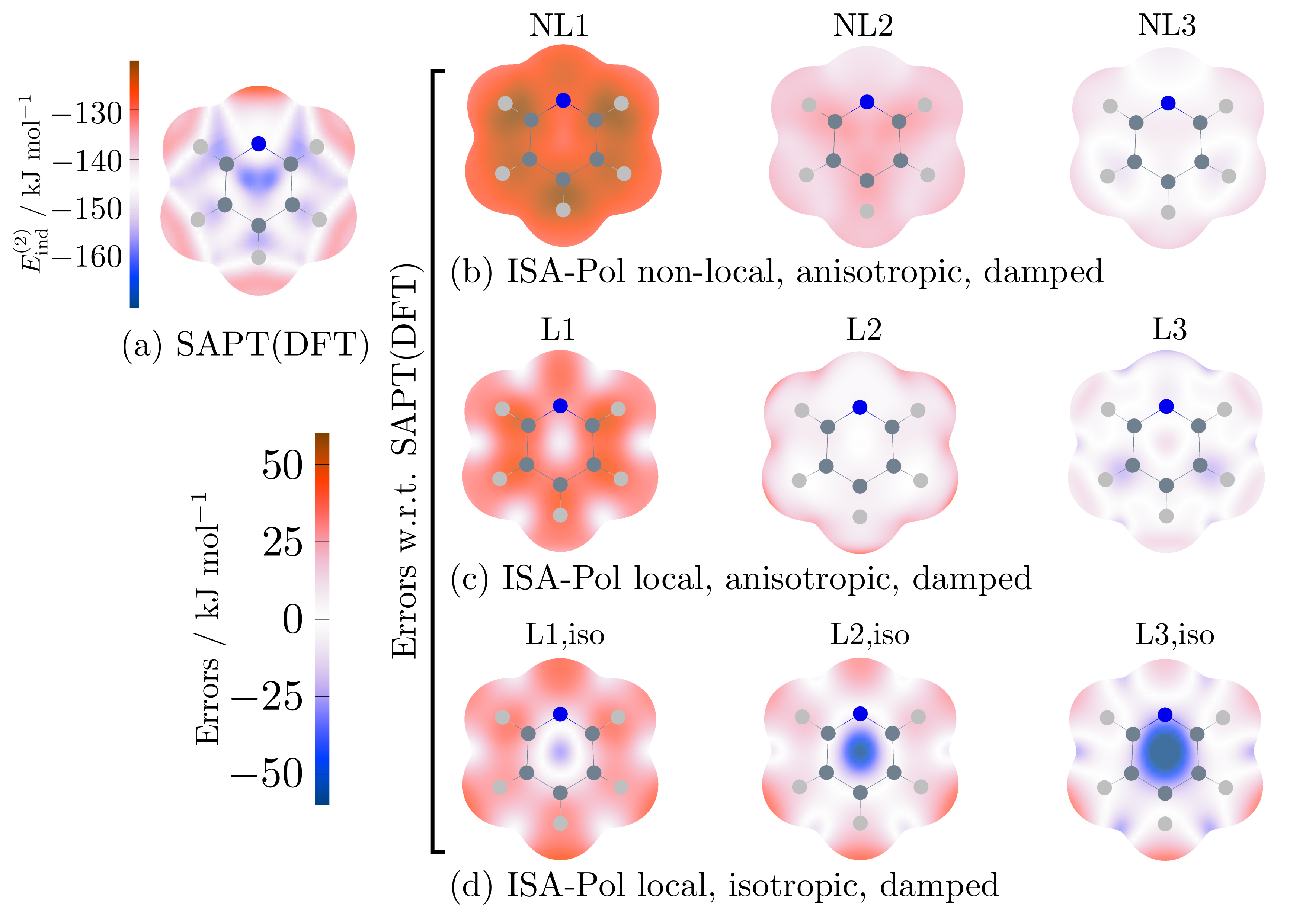
Figure 1: Comparison of the polarization energies for pyridine interacting with a $+1$e point charge on the $0.001$e isodensity surface of pyridine. In panel (a) we visualise the reference SAPT(DFT) second-order induction energies. In the other panels we visualise the errors made by various damped polarization models from the ISA-Pol algorithm: (b) non-local models, (c) localized, anisotropic models, and (d) localized, isotropic models. The maximum rank of the polarizability model is indicated.

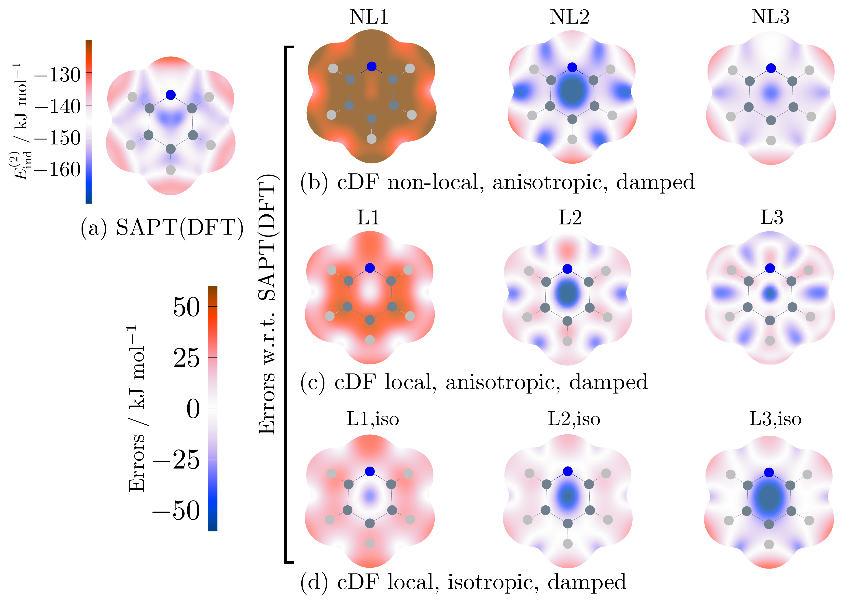
Figure 2: Comparison of the polarization energies for pyridine interacting with a $+1$e point charge on the $0.001$e isodensity surface of pyridine. In panel (a) we visualise the reference SAPT(DFT) second-order induction energies. In the other panels we visualise the errors made by various damped polarization models from the cDF algorithm: (b) non-local models, (c) localized, anisotropic models, and (d) localized, isotropic models. The maximum rank of the polarizability model is indicated.

In Figure 1 we have displayed the reference SAPT(DFT) polarization energies for the pyridine molecule interacting with a $+1$e point charge probe. The energies are displayed on a $10^{-3}$ isodensity surface computed using the CamCASP program. The resulting polarization energies are uncharacteristically large, due both to this choice of surface (which corresponds approximately to the van der Waals surface) and to the large size of the charge: typical local charges in atomic systems will usually be half as much. Also shown in Figure 1 are the errors made by the damped polarization models against the reference energies. Consider first the non-local models: the positive errors made by the NL1 model indicate an underestimation of the polarization energy. The agreement with the reference energies gets progressively and systematically better as the maximum rank increases through 2 to 3. Results for the NL4 model (the maximum rank of the non-local models, and also the most accurate for the choice of damping) are not shown. The localized, anisotropic models exhibit similar errors, but the localized, isotropic models show larger variations in the errors made. In particular, these models shown an underestimation of the polarization near the hydrogen and nitrogen atoms, and a large overestimation of the polarization in the centre of the ring. This is due to the simplicity of the isotropic models: the polarizability of an anisotropic system like pyridine cannot be correctly modelled everywhere using isotropic AIM polarizabilities. As with the distributed multipole moments Misquitta et al. (2014a), the ISA AIMs lead to polarization models with better convergence with increasing rank and fewer artifacts in both the non-local and local models.

In Figure 2 are shown similar results, this time for the models from the cDF algorithm. These differ from the ISA-Pol models in important ways: first of all the errors are larger, even for the non-local models, but perhaps more importantly, the variations in the errors are much larger for all models. It is the latter that is the bigger concern for model building, as variations in errors arise from to position and angle dependent variations in the quality of the model, leading to unreliable predictions.

VI Convergence with basis of the localized models

The next question we need to address is the basis set convergence of the ISA-Pol models. We will not discuss the performance of the non-local or local anisotropic models here as it is difficult to display the data contained in these models in a meaningful and concise manner. Instead we will focus on the local, isotropic models.

The construction of a local, isotropic (frequency-dependent) polarizability model begins with the multipolar localization (see  §III.1) of the ISA-Pol non-local model. This results in an anisotropic, local model which has not yet been refined against the point-to-point polarizabilities. The isotropic model may now be obtained in one of three ways:

• Directly from the unrefined anisotropic model by retaining only the isotropic part of the polarizabilities.

• By refining this isotropic model using the point-to-point polarizabilities.

• By refining the anisotropic model as described in  §III.1 and subsequently retaining only the isotropic part of the polarizabilities.

The second and third options should, in principle, lead to more accurate models. These two approaches lead to similar, but not identical local, isotropic polarizability models. By refining the isotropic models (the second option) we ensure that the resulting isotropic models are the most accurate possible given the limitations imposed. But while this approach may be applicable to small systems for which the isotropic approximation may be valid, it will fail for strongly anisotropic systems for which the third approach may be more appropriate. We have used the second method to obtain the isotropic polarizability models discussed in this paper.

Site	$l$	aDZ	aTZ	aQZ
C1	1	$7.39$	$7.40$	$7.36$
	2	$23.48$	$27.40$	$28.21$
	3	$458.12$	$553.61$	$579.94$
C2	1	$10.53$	$10.62$	$10.64$
	2	$32.58$	$37.75$	$38.85$
	3	$654.79$	$766.85$	$806.50$
S	1	$16.74$	$17.05$	$17.17$
	2	$97.09$	$109.74$	$115.85$
	3	$1449.90$	$1859.26$	$2232.79$
H1	1	$2.18$	$2.17$	$2.18$
	2	$4.41$	$4.44$	$4.74$
	3	$-17.88$	$-6.67$	$-0.36$
H2	1	$1.53$	$1.47$	$1.46$
	2	$4.00$	$4.07$	$4.16$
	3	$-11.64$	$-2.93$	$5.42$

Table 2: Localized, isotropic polarizabilities for the symmetry-distinct sites in the thiophene molecule computed with the WSM algorithm starting from ISA-Pol non-local polarizabilities. The basis sets used are aug-cc-pVDZ (aDZ), aug-cc-pVTZ (aTZ), and aug-cc-pVQZ (aQZ). Atom C1 is the carbon atom attached to the sulfur atom and H1 is the hydrogen atom attached to C1. Atomic units used for all polarizabilities.

In Table 2 we present ISA-Pol localized, isotropic polarizabilities for the symmetry-distinct atoms in the thiophene molecule computed in three basis sets. The dipole–dipole polarizabilities (i.e. rank 1) are already reasonably well converged in the aug-cc-pVDZ basis, with the exception of the sulfur atom which needs the larger aug-cc-pVTZ basis. The quadrupole–quadrupole (rank 2) polarizabilities on the carbon and hydrogen atoms are converged in the aug-cc-pVTZ basis but the aug-cc-pVQZ basis is needed for the sulfur atom. At rank 3, the octopole–octopole polarizabilities on the carbon atoms seem to be approaching convergence in the aug-cc-pVQZ basis, but the sulfur atom is far from convergence. The negative octopole–octopole terms on the hydrogen atoms seem to be a result of the lack of sufficient higher angular terms on these atoms, and of the absence of dipole–quadrupole and quadrupole–octopole polarizabilities in this rather drastic approximation. In the aug-cc-pVQZ basis there is only one negative term present on the H1 atom. Compare these results to those from the cDF approach shown in Table 1. The ISA-Pol algorithm is clearly the more systematic of the two with the AIM local polarizabilities converged or approaching convergence at all ranks.

Dispersion models are obtained from the ISA-Pol-L polarization models computed at imaginary frequency and recombined using methodsWilliams and Stone (2003)^,(Stone, 2013, §4.3.4) implemented in the Casimir module that forms part of the CamCASP suite of programs. While we can compute both anisotropic and isotropic dispersion models, the isotropic models are easier to analyse and use, so we will focus on these only.

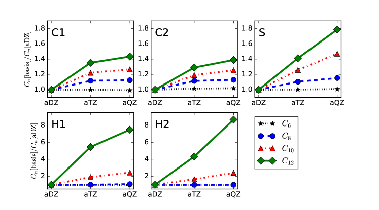
Figure 3: Relative dispersion coefficients for the symmetry-distinct sites in thiophene computed using the localized, isotropic ISA-Pol polarizabilities using the aug-cc-pVDZ (aDZ), aug-cc-pVTZ (aTZ) and aug-cc-pVQZ (aQZ) basis sets. The dispersion coefficients are relative to the values computed in the aug-cc-pVDZ basis.

In Figure 3 we examine the convergence of the distributed dispersion models with basis set. As the dispersion coefficients span many orders of magnitude, we have instead plotted the ratio $C^{aa}_{n}[\text{basis}]/C^{aa}_{n}[\text{aDZ}]$ as a function of basis set used. This allows us to readily determine how the dispersion coefficients vary with increasing basis size. In the case of the two carbon atoms, the $C_{6}$ and $C_{8}$ terms have converged in the aug-cc-pVTZ basis, and the $C_{10}$ and $C_{12}$ terms nearly so in the aug-cc-pVQZ basis. For the two hydrogen atoms the $C_{6}$ and $C_{8}$ terms are converged in the aug-cc-pVDZ basis, but the $C_{10}$ and $C_{12}$ terms are less settled with basis set. This is probably the result of deficiencies in the higher angular part of the hydrogen basis sets, but this needs to be verified. In any case, the higher ranking dispersion terms do not make a significant contribution to the dispersion energy, and have even been fully omitted in some of our earlier models Misquitta and Stone (2008b); Misquitta et al. (2008b). However the same cannot be said for the sulfur atom which is expected to make an important contribution to the dispersion energy due to its large polarizability: here while the $C_{6}$ term is well converged even in the aug-cc-pVDZ basis, the $C_{8}$ term is only just stabilizing in the aug-cc-pVQZ basis, and neither $C_{10}$ nor $C_{12}$ is even close to stabilizing in the largest basis set used. This may be either an artifact of the ISA-Pol algorithm, or a genuine shortcoming of the standard basis sets. Further and more systematic tests on a wider range of systems will be needed to determine the cause of this apparent non-convergence.

Site..Site	$C_{6}$	$C_{8}$	$C_{10}$	$C_{12}$
Pyridine
C1..C1	$1.249(1)$	$3.141(2)$	$1.529(4)$	$4.258(5)$
C2..C2	$3.643(1)$	$6.525(2)$	$3.711(4)$	$8.643(5)$
C3..C3	$2.246(1)$	$5.555(2)$	$2.097(4)$	$5.496(5)$
N..N	$3.206(1)$	$6.735(2)$	$2.609(4)$	$6.196(5)$
H1..H1	$3.533(0)$	$3.407(1)$	$4.384(2)$	$4.795(3)$
H2..H2	$1.802(0)$	$1.758(1)$	$1.921(2)$	$1.880(3)$
H3..H3	$1.689(0)$	$2.306(1)$	$3.392(2)$	$4.173(3)$
Water
O..O	$2.434(1)$	$4.899(2)$	$1.252(4)$	$2.384(5)$
H..H	$0.783(0)$	$4.357(0)$	$9.061(1)$	$7.714(2)$
Methane
C..C	$3.184(1)$	$9.161(2)$	$3.771(4)$	$1.092(6)$
H..H	$2.105(0)$	$2.132(1)$	$3.938(2)$	$4.638(3)$
Thiophene
C1..C1	$2.259(1)$	$5.414(2)$	$2.465(4)$	$6.726(5)$
C2..C2	$3.759(1)$	$8.759(2)$	$4.254(4)$	$1.194(6)$
S..S	$1.082(2)$	$3.895(3)$	$2.096(5)$	$7.904(6)$
H1..H1	$2.096(0)$	$2.453(1)$	$2.864(2)$	$3.021(2)$
H2..H2	$1.268(0)$	$1.630(1)$	$2.518(2)$	$3.207(3)$

Table 3: Localized, isotropic diagonal dispersion coefficients for the symmetry-distinct sites in the pyridine, water, methane, and thiophene dimers computed with the ISA-Pol-L model. The off-diagonal terms, including those between water and methane are provided in the S.I. These results were computed using the d-aug-cc-pVTZ basis with the exception of the thiophine molecule for which we report results computed in the aug-cc-pVQZ basis. Due to the large range of numbers involved, the data are provided in a compact exponential notation with the power of $10$ indicated in parenthesis. That is $x.y(n)=x.y\times 10^{n}$. Atomic units used for all dispersion coefficients.

In Table 3 we report the ISA-Pol-L isotropic dispersion coefficients for the symmetry-distinct sites in the water, methane, pyridine and thiophene molecules. Only the diagonal, that is same-site, terms are reported: the complete dispersion models for these molecules and also those for the methane..water complex are given in the S.I. Notice that while the dispersion coefficients for the carbon atoms in these molecules are of similar magnitude, they nevertheless vary considerably in accordance with what might be expected from the variations in the local chemical environment. For example, the C1 atom in pyridine and the C1 atom in thiophene both have smaller dispersion coefficients than the other carbon atoms in the molecules, which should be expected as these atoms are bonded directly to the more electronegative N and S atoms in the respective molecules. Likewise, while the dispersion terms on the hydrogen atoms are similar, those on the hydrogen atom in water are substantially smaller due to the large electronegativity of the oxygen atom in the water molecule. The ability of the ISA-Pol-L models to provide dispersion terms from $C_{6}$ to $C_{12}$ which respond to the chemical environment of the atoms in the molecule could be used to develop more detailed and comprehensive models for the dispersion energy, but more extensive data sets will be needed for a full analysis.

VI.1 Assessing the models using SAPT(DFT)

The ultimate test of any dispersion model is how well it is able to match the reference dispersion energies. Here, as with the polarization models, there is the issue of damping, without which meaningful comparisons can only be made at large intermolecular separations where the damping is negligible. However such a comparison is not useful from the practical point of view as we are usually interested in the performance of the models at energetically important configuration, that is, in the region of the energy minimum. Consequently we do need to address the issue of damping, but as this is not the focus of this paper, we will limit the present discussion to the familiar Tang–Toennies Tang and Toennies (1984) damping functions:

$$f_{n}(x) =1-e^{-x}\sum_{k=0}^{n}\frac{x^{k}}{k!},$$ (23)

where the order $n$ corresponds with the rank in the dispersion expansion Stone (2013) and $x$ is a function of the site–site distance and the damping coefficient. The damping models we have used differ in the definition of $x$ as follows:

• Ionization potential (IP) damping Misquitta and Stone (2008b):

  $$x_{ab} =\left(\sqrt{2I_{A}}+\sqrt{2I_{B}}\right)r_{ab}=\beta_{AB}r_{ab},$$ (24)

  where $I_{A}$ and $I_{B}$ are the vertical ionization energies, in a.u., of the two interacting molecules. This is the simplest of the damping models with one damping parameter for all pairs of sites $(a,b)$ between the interacting molecules $A$ and $B$.

• The Slater damping from Van Vleet et al. Van Vleet et al. (2016). Here the damping parameter is dependent on the pairs of interacting atoms and is given by

  $$x_{ab} =\beta_{ab}r_{ab}-\frac{\beta_{ab}(2\beta_{ab}r_{ab}+3)}{\beta_{ab}^{2}r_{ab}^{2}+3\beta_{ab}r_{ab}+3},$$ (25)

  where the parameter $\beta_{ab}$ is now dependent on the sites and is defined as $\beta_{ab}=\sqrt{\beta_{a}\beta_{b}}$, where the parameter $\beta_{a}$ is extracted from the ISA shape function $w^{a}$ by fitting it to an exponential of the form $K\exp{(-\beta_{a}r)}$, and $\beta_{b}$ likewise. Misquitta et al. (2014a); Van Vleet et al. (2016). This damping function is motivated by the form of the overlap of two such Slater exponentialsVan Vleet et al. (2016).

• The scaled ISA damping model is a simplification of the Slater damping model. Here we define a scaled parameter $\tilde{\beta}_{a}$ for each site in molecule $A$ as follows:

  $$\tilde{\beta}_{a} =s_{A}\beta_{a},$$ (26)

  where $\beta_{a}$ is defined above and $s_{A}$ is the molecule-specific empirical scaling parameter. Next we define $\beta_{ab}$ from the combination rule

  $$\beta_{ab} =\sqrt{\tilde{\beta}_{a}\tilde{\beta}_{b}},$$ (27)

  and $x_{ab}=\beta_{ab}r_{ab}$. In Ref. 2 the scaling parameter is taken to be a constant $s=0.84$ independent of the type of molecule, but here we allow the parameter to vary according to the molecule and determine it empirically by fitting the model energies to the reference dispersion energies.

In the comparisons of the ISA-Pol-L dispersion models that we now discuss, the reference dispersion energies used in the comparisons have been computed using SAPT(DFT) and are defined as

$$E^{(2)}_{\rm DISP} =E^{(2)}_{\rm disp,pol}+E^{(2)}_{\rm disp,exch}.$$ (28)

All dispersion models are computed from isotropic ISA-Pol-L polarizabilities, consequently we should expect errors for systems with a strong anisotropy. In all cases the isotropic ISA-Pol-L dispersion models contain even terms from $C_{6}$ to $C_{12}$ on all atoms.

In Figure 4 we display dispersion energies for the methane dimer in more than 2600 dimer configurations. Because the methane molecule has high symmetry and indeed is nearly spherical, we should expect the dispersion energy of this system to be well approximated by an isotropic dispersion model. This is indeed the case, and we see nearly perfect correlation of the ISA-Pol-L dispersion energies with the scaled damping model with the reference energies. In this case a scaling parameter of $0.76$ was determined. On the other hand, the IP damping model which we have recommended in the past does not provide sufficient damping, and nor does the Slater model, though it is better.

Figure 5 shows data for the water dimer in more than 2000 dimer configurations. Water is a more anisotropic system than methane, and we cannot expect the isotropic models to behave as well for water dimer as for methane dimer. Once again both the IP and Slater damping models result in underdamping, though not as severely as for methane dimer. The scaled damping model with a scaling factor of $0.76$ fares far better, resulting in dispersion energies for most of the dimers within $\pm 5$% from the reference energies. In Figure 6 we have displayed dispersion energies for the mixed methane$\cdot\!\cdot\!\cdot$water system. The picture is the same, with the scaled damping model correlating very well with the reference energies.

In Figure 7 we display dispersion energies for the pyridine dimer in over 700 configurations taken from data sets 1 and 2 from Ref. 1. The pyridine molecule is the most anisotropic one we have considered in this paper and we may therefore expect to see a relatively large scatter in the model dispersion energies. This is indeed the case: while the scaled damping dispersion model still results in the best dispersion energies, these now deviate from the reference energies by slightly more than $5$%. The scaling parameter has been determined to be $0.71$ which is smaller than the values obtained for the water and methane systems, and considerably smaller than the value of $0.84$ recommended by Van Vleet et al. Van Vleet et al. (2016) Part of the reason for this is that the AIM densities for the pyridine molecule are themselves strongly anisotropic due to the $\pi$-electron density of the molecule, but the parameters $\beta_{a}$ used in eq. (26) are obtained from the isotropic shape functions and therefore the correct AIM density decay is not obtained. Instead the anisotropic AIM densities $\rho^{a}$ should be used, and we are currently investigating this possibility. Curiously, for this system the IP damping model is quite similar to the scaled damping, but the Slater damping model once again under-damps.

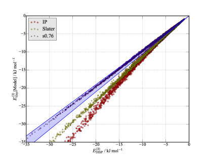
Figure 4: Dispersion energies for the methane dimer in a variety of configurations. Reference energies are computed using SAPT(DFT) as described in the text. The ISA-Pol dispersion models are all isotropic and are damped with various damping models: ‘IP’ refers to the Tang–Toennies damping with a single damping parameter determined using the molecular ionization potentials, ‘Slater’ refers to the damping model from the Slater-FF model with exponents determined using the ISA, and ‘s0.76’ refers to the Tang–Toennies damping with atom-pair-dependent damping parameters determined using the ISA and scaled by $0.76$ as described in the text. The light blue bar represents $\pm 5$% errors compared with the reference dispersion energies.

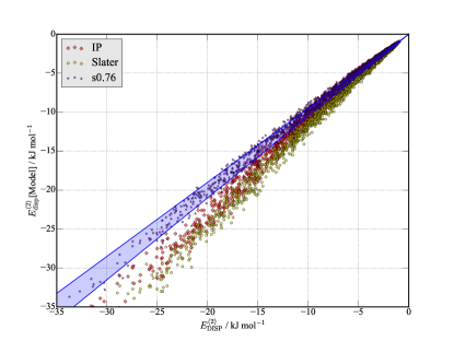
Figure 5: Dispersion energies for the water dimer in a variety of configurations. Reference energies are computed using SAPT(DFT) as described in the text. The ISA-Pol dispersion models are all isotropic and are damped with various damping models which are described in the caption to Figure 4.

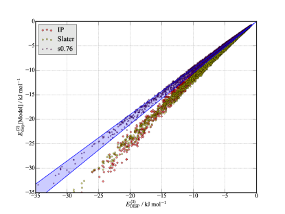
Figure 6: Dispersion energies for the methane..water dimer in a variety of configurations. Reference energies are computed using SAPT(DFT) as described in the text. The ISA-Pol dispersion models are all isotropic and are damped with various damping models which are described in the caption to Figure 4.

Figure 7: Dispersion energies for the pyridine dimer in a variety of configurations. Reference energies are computed using SAPT(DFT) as described in the text. The ISA-Pol dispersion models are all isotropic and are damped with various damping models which are described in the caption to Figure 4.

VI.2 Convergence with rank

Although it is reasonably well known that the dispersion expansion should include terms beyond $C_{6}$, it is perhaps not as well appreciated just how many terms are required for this expansion to converge (when appropriately damped). We have explored this issue in a previous paper Misquitta and Stone (2008b), where we concluded that models including terms to at least $C_{10}$ were needed to achieve sufficiently good agreement with SAPT(DFT). In Figure 8 we present even more extensive data for the methane dimer which clearly demonstrates that the $C_{6}$-only models commonly used in simple force-fields, and indeed in many dispersion corrections to density-functional theory, severely underestimate the dispersion energy from SAPT(DFT). For this dimer, we need to include terms to $C_{10}$ before we begin to agree with the reference energies to within 5%.

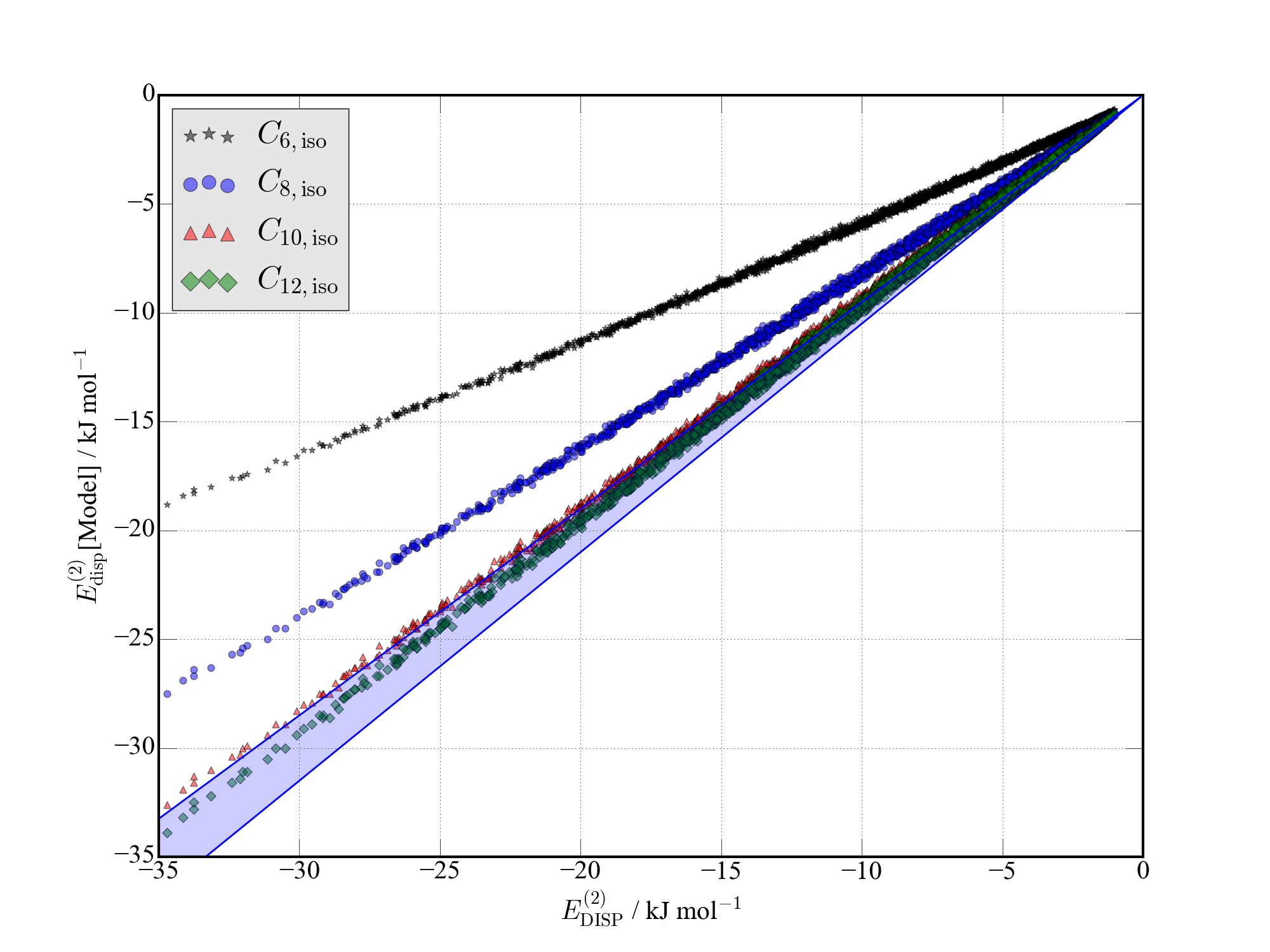
Figure 8: Dispersion energies for the methane dimer from ISA-Pol isotropic dispersion models at various maximum ranks. All models are damped using the scaled Tang–Toennies damping with scaling $0.76$.

VI.3 Combination rules

Dispersion models in common intermolecular interaction models are usually constructed to satisfy combination rules, usually through a constrained fitting process (see for example Ref. 42). This has the advantage of greatly reducing the number of parameters in the model, and the most commonly used geometric mean combination rule has good justification from theory, although the actual dispersion coefficients may not satisfy a combination rule accurately.

The geometric mean combination rule defines the mixed site $C^{ab}_{n}$ dispersion coefficients as follows:

$$C^{ab}_{n}=\sqrt{C^{aa}_{n}\,C^{bb}_{n}},$$ (29)

where $C^{aa}_{n}$ and $C^{bb}_{n}$ are the same-site coefficients. This combination rule may be derived for the $n=6$ terms Mavroyannis and Stephen (1962) from the exact expression for the isotropic $C^{ab}_{6}$ coefficient:

$$C^{ab}_{6} =\frac{3}{\pi}\int_{0}^{\infty}\bar{\alpha}^{a}(iv)\bar{\alpha}^{b}(iv)dv,$$ (30)

by using the single-pole approximation to the isotropic frequency-dependent polarizabilities

$$\bar{\alpha}(iv) =\bar{\alpha}(0)\frac{v_{0}^{2}}{v^{2}+v_{0}^{2}},$$ (31)

where $v_{0}$ is the pole. We additionally have to assume that the poles for the two sites $a$ and $b$ are similar, that is, $v_{0}^{a}\approx v_{0}^{b}$. This is identical to the Unsöld average energy approximation Stone (2013). The advantages of this combination rule are apparent: for a system of $N$ interacting sites, only $\mathcal{O}(N)$ dispersion coefficients would be needed, rather than the $\mathcal{O}(N^{2})$ needed without such a rule.

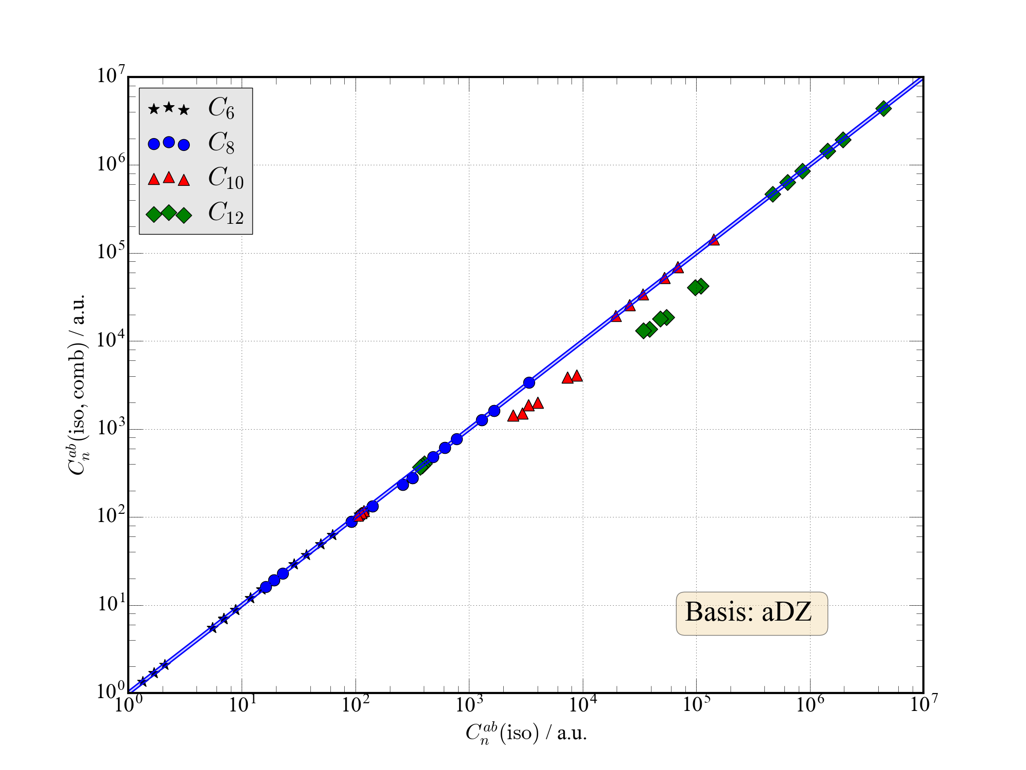
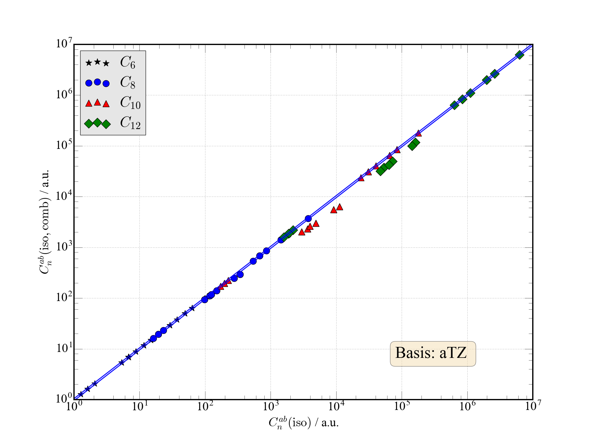
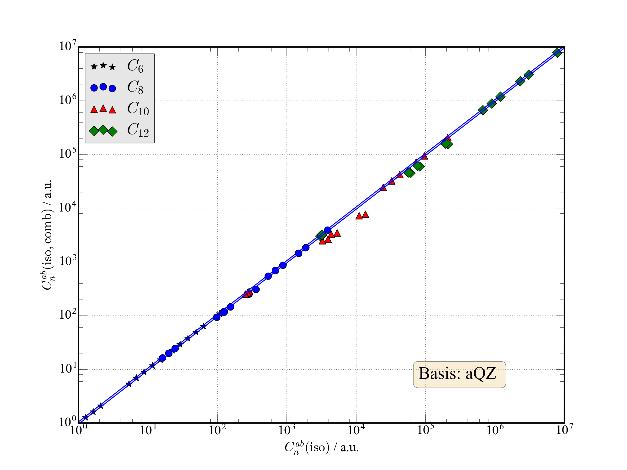
Figure 9: Comparison of ISA-Pol dispersion coefficients for thiophene against those obtained using the geometric mean combination rule. The three panels show how the combination rules are satisfied as a function of the basis set used to obtain the ISA-Pol isotropic dispersion models. In all cases the points off the diagonal line are associated with the hydrogen atoms in thiophene.

Do the ISA-Pol dispersion models satisfy the geometric mean combination rule? Once again this question is a complex one if we account for the angular variation of the dispersion parameters, so here we will restrict this discussion to the isotropic dispersion models only. In Figure 9 we plot the dispersion coefficients for the thiophene molecule computed using the geometric mean combination rule against reference ISA-Pol-L isotropic dispersion coefficients. This is done for the aug-cc-pV$n$Z, $n=\text{D,T,Q}$ basis sets. It can be seen that the ISA-Pol-L models satisfy the combination rule very well for $n=6,8,10,12$, that is for all ranks of the dispersion coefficients considered in this paper. In all cases, the terms that are most in error are those involving at least one of the hydrogen atoms, but these errors are reduced as the basis set gets larger, echoing the trend to more well-defined polarizabilities seen in Table 2.

This property of the dispersion models derived from ISA-Pol-L polarizabilities seems to hold for a variety of systems, though less well for those containing a larger fraction of hydrogen atoms. This is remarkable given that the combination rules are never imposed, and there is no reason to expect the single-pole approximation to hold, or indeed for the poles on different atoms to be similar. Further work is needed to analyse exactly why this is the case, and if and when it breaks down, but this property of the ISA-Pol-L models, if generally applicable, will be a very useful feature for the development of models of more diverse interactions.

VII Analysis & Outlook

We have described and implemented the ISA-Pol algorithm for computing distributed frequency-dependent polarizabilities and dispersion coefficients for molecular systems. This algorithm is based on a basis-space implementation Misquitta et al. (2014a) of the iterated stockholder atoms (ISA) algorithm of Lillestolen and Wheatley Lillestolen and Wheatley (2008). We have described a simpler and more versatile implementation of the BS-ISA algorithm and have implemented this algorithm in a developer’s version of CamCASP 6.0. This new algorithm allows for higher accuracies in the ISA solution and in the resulting distributed properties. Additionally the algorithm has a computational cost that scales linearly with the system size.

The ISA-Pol algorithm results in non-local distributed polarizabilities which can be localized to result in approximate atomic polarizabilities using schemes we have discussed and demonstrated. The resulting models have many of the desired properties discussed in the Introduction. The most important of these are:

• Systematic convergence of the ISA-Pol non-local polarizabilities as a function of rank. This model has been demonstrated to converge more systematically than the constrained density fitting, cDF, model we have previously proposed Misquitta and Stone (2006), and also the related SRLO algorithm from Rob & Szalewicz Rob and Szalewicz (2013).

• The localized ISA-Pol polarizabilities (ISA-Pol-L) are well defined and are usually positive definite where local models can give a good account of what are inherently non-local effects. In other words, for systems with relatively short electron correlation lengths, the ISA-Pol-L models are appropriate and systematic and lead to reasonably accurate polarization energies.

• We have demonstrated that the ISA-Pol-L polarizabilities converge systematically with basis set and appear to have a well-defined basis set limit. The systematic behaviour of these distributed polarizabilities should make it possible to extrapolate the polarizabilities of the atoms-in-the-molecule (AIMs) to the complete basis set limit. This was not possible with the WSM models Misquitta and Stone (2008a); Misquitta et al. (2008a) built from cDF non-local polarizabilities as has been illustrated in the Introduction.

• Dispersion models constructed from the ISA-Pol-L frequency-dependent polarizabilities are well defined and, when suitably damped, show exceptionally good reproduction of theSAPT(DFT) dispersion energies for a variety of anisotropic systems.

• Damping of the dispersion models is achieved using the Tang–Toennies functions with atom-specific damping parameters derived using the BS-ISA algorithm. A single scaling parameter is used as described by Van Vleet et al. Van Vleet et al. (2016), though we have allowed the scaling parameter to vary with the molecule.

• The isotropic dispersion coefficients from the ISA-Pol-L algorithm have been shown to satisfy the geometric mean combination rule that is used in many empirical models for the dispersion energy, but is not imposed at any stage in developing the localized ISA-Pol polarizabilities. This is the case for terms from $C_{6}$ to $C_{12}$ and the accuracy of the combination rule improves with increase in the basis set used for the ISA-Pol calculation.

These properties alone make the ISA-Pol and associated localized ISA-Pol-L models promising candidates for developing detailed and accurate polarization and dispersion models for intermolecular interactions. At present, these methods are limited to closed-shell molecules, but this is to a large extent a limitation of the implementation in the CamCASP 6.0 program.

Amongst the issues that we have not yet resolved adequately are the determination of the damping of the polarization and dispersion models, and the problem of the anisotropy of the dispersion models. The polarization damping question has been raised by one of us elsewhere Misquitta (2013) but it needs to be re-visited in context of the ISA-Pol models for which the damping needed is clearly different from models derived from the cDF polarizabilities (see  §V.1). The damping models introduced by Van Vleet et al. Van Vleet et al. (2016) are definitely promising. In particular, we have shown that the scaled ISA damping model can result in dispersion energies that agree with the reference SAPT(DFT) total dispersion energy, $E^{(2)}_{\rm DISP}$, to 5% or better. In fact, for the methane dimer the agreement is much better than 5%, and also substantially better than that achieved by a recently proposed anisotropic LoProp-based dispersion model Harczuk et al. (2017). However there remains the question of how this can be improved and it seems like there are a few issues that need to be investigated:

• Anisotropy in the damping: Perhaps the damping coefficients need to be extracted from the ISA AIM densities $\rho^{a}$ rather than from the ISA shape functions $w^{a}$ as we do currently. This would have the consequence of making the damping parameters anisotropic and these may be more appropriate at modelling interactions involving sites that are themselves strongly anisotropic. This would be the case for the oxygen atom in water and for the carbon atoms in a $\pi$-conjugated system.

• Anisotropy in the dispersion coefficients: The dispersion models derived from the ISA-Pol-L polarizabilities include anisotropy, but we have, as yet, focused only on the isotropic parts of these models. This has been done mainly for computational reasons: most simulation codes accept only isotropic dispersion models, and the anisotropic models tend to be very complex. Recently, Van Vleet et al. Van Vleet et al. (2018) have demonstrated how the inclusion of atomic anisotropy can result in a rather significant improvement in the model energies, but this approach is empirical in the sense that the anisotropy parameters are determined by fitting to reference SAPT(DFT) dispersion energies. We need a way to develop practical models in a non-empirical manner.

We have not investigated the transferability of the ISA-Pol polarizabilities as these are not the fundamental AIM polarizabilities, but are effective atomic polarizabilities after through-space polarization in the Applequist sense Applequist et al. (1972); Stone (2013) has been taken into account. It should however be possible to derive the ‘bare’ AIM polarizabilities from those computed from ISA-Pol and this is something we are currently exploring. Finally, the fundamental relation of the ISA-Pol models with the underlying ISA decomposition may eventually lead to the development of approximations that allow the models to be mapped onto the properties of the ISA AIM densities. If possible, this would significantly increase our ability to easily construct polarization models for complex molecular system, especially those too large for routine linear-response calculations in a large enough basis set. This too is something we are currently exploring.

VIII Acknowledgements

We dedicate this article to the memory of Dr János Ángyán for a friendship and for many scientific discussions, one of which led to the ISA-Pol method. AJM thanks Queen Mary University of London for support and the Thomas Young Centre for a stimulating environment, and also the Université de Lorraine for a visiting professorship during which part of this work was completed. We also thank Dr Rory A. J. Gilmore for assistance in calculating the SAPT(DFT) reference energies for the water..water, methane..methane, and water..methane complexes. We thank Dr Toon Verstraelen for helpful comments on the manuscript.

IX Additional information

All developments have been implemented in a developer’s version of the CamCASP 6.0 Misquitta and Stone (2018) program which may be obtained from the authors on request. CamCASP has been interfaced to the DALTON 2.0 (2006 through to 2015), NWChem 6.x, GAMESS(US) , and Psi4 1.1 programs. The supplementary information (SI) contains additional data from the systems we have investigated but not included in this paper.

References

- Misquitta and Stone (2016) A. J. Misquitta and A. J. Stone, Journal of Chemical Theory and Computation 12, 4184 (2016), pMID: 27467814, https://doi.org/10.1021/acs.jctc.5b01241 .
- Van Vleet et al. (2016) M. J. Van Vleet, A. J. Misquitta, A. J. Stone, and J. R. Schmidt, J. Chem. Theory Comput. 12, 3851 (2016), pMID: 27337546, https://doi.org/10.1021/acs.jctc.6b00209 .
- Metz et al. (2016) M. P. Metz, K. Piszczatowski, and K. Szalewicz, J. Chem. Theory Comput. 12, 5895 (2016).
- Vandenbrande et al. (2017) S. Vandenbrande, M. Waroquier, V. V. Speybroeck, and T. Verstraelen, Journal of Chemical Theory and Computation 13, 161 (2017).
- Van Vleet et al. (2018) M. J. Van Vleet, A. J. Misquitta, and J. R. Schmidt, J. Chem. Theory Comput. 14, 739 (2018).
- Mas et al. (1997) E. M. Mas, K. Szalewicz, R. Bukowski, and B. Jeziorski, J. Chem. Phys. 107, 4207 (1997).
- Korona et al. (1997) T. Korona, H. L. Williams, R. Bukowski, B. Jeziorski, and K. Szalewicz, J. Chem. Phys. 106, 5109 (1997).
- Bukowski et al. (1999a) R. Bukowski, K. Szalewicz, and C. Chabalowski, J. Phys. Chem. A 103, 7322 (1999a).
- Chang et al. (2003) B. Chang, O. Akin-Ojo, R. Bukowski, and K. Szalewicz, J. Chem. Phys. 119, 11654 (2003).
- Misquitta et al. (2000) A. J. Misquitta, R. Bukowski, and K. Szalewicz, J. Chem. Phys. 112, 5308 (2000).
- Murdachaew et al. (2001) G. Murdachaew, A. J. Misquitta, R. Bukowski, and K. Szalewicz, J. Chem. Phys. 114, 764 (2001).
- Stone and Misquitta (2007) A. J. Stone and A. J. Misquitta, Int. Revs. Phys. Chem. 26, 193 (2007).
- Stone (2013) A. J. Stone, The Theory of Intermolecular Forces, 2nd ed. (Oxford University Press, Oxford, 2013).
- Rob and Szalewicz (2013) F. Rob and K. Szalewicz, Chem. Phys. Lett. 572, 146 (2013).
- Gagliardi et al. (2004) L. Gagliardi, R. Lindh, and G. Karlstrom, J. Chem. Phys. 121, 4494 (2004).
- Harczuk et al. (2017) I. Harczuk, B. Nagy, F. Jensen, O. Vahtras, and H. Ågren, Physical Chemistry Chemical Physics (2017), 10.1039/C7CP02399E.
- Misquitta and Stone (2006) A. J. Misquitta and A. J. Stone, J. Chem. Phys. 124, 024111 (2006).
- Misquitta and Stone (2008a) A. J. Misquitta and A. J. Stone, J. Chem. Theory Comput. 4, 7 (2008a).
- Misquitta et al. (2008a) A. J. Misquitta, A. J. Stone, and S. L. Price, J. Chem. Theory Comput. 4, 19 (2008a).
- Angyan et al. (1994) J. G. Angyan, G. Jansen, M. Loos, C. Hattig, and B. A. Hess, Chem. Phys. Lett. 219, 267 (1994).
- Dehez et al. (2001) F. Dehez, C. Chipot, C. Millot, and J. G. Angyan, Chem. Phys. Lett. 338, 180 (2001).
- Jansen et al. (1996) G. Jansen, C. Hattig, B. A. Hess, and J. G. Angyan, Mol. Phys. 88, 69 (1996).
- Angyan et al. (2003) J. G. Angyan, C. Chipot, F. Dehez, C. Hattig, G. Jansen, and C. Millot, J. Comp. Chem. 24, 997 (2003).
- Lillestolen and Wheatley (2007) T. C. Lillestolen and R. J. Wheatley, J. Phys. Chem. A 111, 11141 (2007).
- Wheatley and Lillestolen (2008) R. J. Wheatley and T. C. Lillestolen, Mol. Phys. 106, 1545 (2008).
- Wheatley and Mitchell (1994) R. J. Wheatley and J. B. O. Mitchell, J. Comp. Chem. 15, 1187 (1994).
- Chaudret et al. (2014) R. Chaudret, N. Gresh, C. Narth, L. Lagardère, T. A. Darden, G. A. Cisneros, and J.-P. Piquemal, The Journal of Physical Chemistry A 118, 7598 (2014).
- Vigné-Maeder and Claverie (1988) F. Vigné-Maeder and P. Claverie, J. Chem. Phys. 88, 4934 (1988).
- Mas et al. (2000) E. M. Mas, R. Bukowski, K. Szalewicz, G. C. Groenenboom, P. E. S. Wormer, and A. van der Avoird, J. Chem. Phys. 113, 6687 (2000).
- Fang et al. (2013) H. Fang, M. T. Dove, L. H. N. Rimmer, and A. J. Misquitta, Phys. Rev. B 88, 104306 (2013).
- Bader (1990) R. Bader, Atoms in Molecules (Clarendon Press, Oxford, 1990).
- Hirshfeld (1977) F. L. Hirshfeld, Theoretica chimica acta 44, 129 (1977).
- Lillestolen and Wheatley (2008) T. C. Lillestolen and R. J. Wheatley, Chem. Commun. 2008, 5909 (2008).
- Bultinck et al. (2009) P. Bultinck, D. L. Cooper, and D. V. Neck, Phys. Chem. Chem. Phys. 11, 3424 (2009).
- Parr et al. (2005) R. G. Parr, P. W. Ayers, and R. F. Nalewajski, J. Phys. Chem. A 109, 3957 (2005).
- Matta and Bader (2006) C. F. Matta and R. F. W. Bader, J. Phys. Chem. A 110, 6365 (2006).
- Stone (1981) A. J. Stone, Chem. Phys. Lett. 83, 233 (1981).
- Stone (2005) A. J. Stone, J. Chem. Theory Comput. 1, 1128 (2005).
- Söderhjelm et al. (2007) P. Söderhjelm, J. W. Krogh, G. Karlström, U. Ryde, and R. Lindh, Journal of Computational Chemistry 28, 1083 (2007).
- Piquemal et al. (2006) J.-P. Piquemal, G. A. Cisneros, P. Reinhardt, and N. Gresh, J. Chem. Phys. 124, 104101 (2006).
- Sebetci and Beran (2010) A. Sebetci and G. J. O. Beran, J. Chem. Theory Comput. 6, 155 (2010).
- McDaniel and Schmidt (2013) J. G. McDaniel and J. Schmidt, J. Phys. Chem. A 117, 2053 (2013).
- Menendez et al. (2015) M. Menendez, A. Martín Pendas, B. Braida, and A. Savin, Computational and Theoretical Chemistry Special Issue: Understanding structure and reactivity from topology and beyond, 1053, 142 (2015).
- Kosov and Popelier (2000) D. S. Kosov and P. L. A. Popelier, 104, 7339 (2000).
- Popelier and Rafat (2003) P. L. A. Popelier and M. Rafat, Chem. Phys. Lett. 376, 148 (2003).
- Hattig et al. (1997) C. Hattig, G. Jansen, B. A. Hess, and J. G. Angyan, Mol. Phys. 91, 145 (1997).
- Ayers (2006) P. W. Ayers, Theor. Chim. Acta 115, 370 (2006).
- Bultinck et al. (2007) P. Bultinck, C. Van Alsenoy, P. W. Ayers, and R. Carbó-Dorca, J. Chem. Phys. 126, 144111 (2007).
- Verstraelen et al. (2012) T. Verstraelen, P. Ayers, V. V. Speybroeck, and M. Waroquier, Chem. Phys. Lett. 545, 138 (2012).
- Misquitta et al. (2014a) A. J. Misquitta, A. J. Stone, and F. Fazeli, J. Chem. Theory Comput. 10, 5405 (2014a).
- Misquitta and Stone (2018) A. J. Misquitta and A. J. Stone, “CamCASP: a program for studying intermolecular interactions and for the calculation of molecular properties in distributed form,” University of Cambridge (2018), accessed: May 2018.
- Stone (1985) A. J. Stone, Mol. Phys. 56, 1065 (1985).
- Misquitta et al. (2010) A. J. Misquitta, J. Spencer, A. J. Stone, and A. Alavi, Phys. Rev. B 82, 075312 (2010).
- Liu et al. (2011) R.-F. Liu, J. G. Angyan, and J. F. Dobson, J. Chem. Phys. 134, 114106 (2011).
- Misquitta et al. (2014b) A. J. Misquitta, R. Maezono, N. D. Drummond, A. J. Stone, and R. J. Needs, Physical Review B 89, 045140 (2014b).
- Casida (1995) M. E. Casida, in Recent Advances in Density-Functional Theory, edited by D. P. Chong (World Scientific, 1995) p. 155.
- Colwell et al. (1995) S. M. Colwell, N. C. Handy, and A. M. Lee, Phys. Rev. A 53, 1316 (1995).
- Dunlap et al. (1979) B. I. Dunlap, J. W. D. Connolly, and J. R. Sabin, J. Chem. Phys. 71, 4993 (1979).
- Dunlap (2000) B. I. Dunlap, Phys. Chem. Chem. Phys. 2, 2113 (2000).
- Jamorski et al. (1995) C. Jamorski, M. E. Casida, and D. R. Salahub, J. Chem. Phys. 104, 5134 (1995).
- Misquitta et al. (2003) A. J. Misquitta, B. Jeziorski, and K. Szalewicz, Phys. Rev. Lett. 91, 33201 (2003).
- Hesselmann et al. (2005) A. Hesselmann, G. Jansen, and M. Schütz, J. Chem. Phys. 122, 014103 (2005).
- Lillestolen and Wheatley (2009) T. C. Lillestolen and R. J. Wheatley, J. Chem. Phys. 131, 144101 (2009).
- Le Sueur and Stone (1994) C. R. Le Sueur and A. J. Stone, Mol. Phys. 83, 293 (1994).
- Williams and Stone (2003) G. J. Williams and A. J. Stone, J. Chem. Phys. 119, 4620 (2003).
- Helgaker et al. (2005) T. Helgaker, H. J. A. Jensen, P. Joergensen, J. Olsen, K. Ruud, H. Aagren, A. Auer, K. Bak, V. Bakken, O. Christiansen, S. Coriani, P. Dahle, E. K. Dalskov, T. Enevoldsen, B. Fernandez, C. Haettig, K. Hald, A. Halkier, H. Heiberg, H. Hettema, D. Jonsson, S. Kirpekar, R. Kobayashi, H. Koch, K. V. Mikkelsen, P. Norman, M. J. Packer, T. B. Pedersen, T. A. Ruden, A. Sanchez, T. Saue, S. P. A. Sauer, B. Schimmelpfennig, K. O. Sylvester-Hvid, P. R. Taylor, and O. Vahtras, “Dalton, a molecular electronic structure program, release 2.0,” (2005), see http://www.kjemi.uio.no/software/dalton/dalton.html.
- Adamo and Barone (1999) C. Adamo and V. Barone, J. Chem. Phys. 110, 6158 (1999).
- Fermi and Amaldi (1934) E. Fermi and E. Amaldi, “Le orbite s delgi elementi,” in Memorie della Classe di scienze fisiche della Reale Accademia d’Italia, Vol. 6(1) (Reale Accademia d’Italia, 1934) pp. 119–149.
- Misquitta et al. (2005) A. J. Misquitta, R. Podeszwa, B. Jeziorski, and K. Szalewicz, J. Chem. Phys. 123, 214103 (2005).
- Perdew and Wang (1992) J. P. Perdew and Y. Wang, Phys. Rev. B 45, 13244 (1992).
- (71) S. G. Lias, “Ionization energy evaluation in nist chemistry webbook, nist standard reference database number 69, eds. w. g. mallard and p. j. linstrom, gaithersburg, 2000 (http://webbook.nist.gov),” Accessed: Oct 2013.
- Mas and Szalewicz (1996) E. M. Mas and K. Szalewicz, J. Chem. Phys. 104, 7606 (1996).
- Nakata and Kuchitsu (1986) M. Nakata and K. Kuchitsu, J. Chem. Soc. Jpn. , 1446 (1986).
- Akin-Ojo and Szalewicz (2005) O. Akin-Ojo and K. Szalewicz, J. Chem. Phys. 123, 134311 (2005).
- Kendall et al. (1992) R. A. Kendall, T. H. Dunning, Jr., and R. J. Harrison, J. Chem. Phys. 96, 6796 (1992).
- Valiev et al. (2010) M. Valiev, E. J. Bylaska, N. Govind, K. Kowalski, T. P. Straatsma, H. J. J. Van Dam, D. Wang, J. Nieplocha, E. Apra, T. L. Windus, and W. A. de Jong, Computer Physics Communications 181, 1477 (2010).
- Sadlej (1988) A. J. Sadlej, Coll. Czech Chem. Commun. 53, 1995 (1988).
- Bukowski et al. (1999b) R. Bukowski, J. Sadlej, B. Jeziorski, P. Jankowski, K. Szalewicz, S. A. Kucharski, H. L. Williams, and B. M. Rice, J. Chem. Phys. 110, 3785 (1999b).
- Weigend et al. (2002) F. Weigend, A. Kohn, and C. Hattig, J. Chem. Phys. 116, 3175 (2002).
- Misquitta (2013) A. J. Misquitta, J. Chem. Theory Comput. 9, 5313 (2013).
- Tang and Toennies (1984) K. T. Tang and J. P. Toennies, J. Chem. Phys. 80, 3726 (1984).
- Misquitta and Stone (2008b) A. J. Misquitta and A. J. Stone, Mol. Phys. 106, 1631 (2008b).
- Misquitta et al. (2008b) A. J. Misquitta, G. W. A. Welch, A. J. Stone, and S. L. Price, Chem. Phys. Lett. 456, 105 (2008b).
- Mavroyannis and Stephen (1962) C. Mavroyannis and M. J. Stephen, Mol. Phys. 5, 629 (1962).
- Applequist et al. (1972) J. Applequist, J. R. Carl, and K.-K. Fung, J. Am. Chem. Soc. 94, 2952 (1972).