Study of the superconducting order parameter in the negative-$U$ 2D-Hubbard model by grand-canonical twist-averaged boundary conditions

Abstract

By using variational Monte Carlo and auxiliary-field quantum Monte Carlo methods, we perform an accurate finite-size scaling of the $s$-wave superconducting order parameter and the pairing correlations for the negative-$U$ Hubbard model at zero temperature in the square lattice. We show that the twist-averaged boundary conditions (TABCs) are extremely important to control finite-size effects and to achieve smooth and accurate extrapolations to the thermodynamic limit. We also show that TABCs is much more efficient in the grand-canonical ensemble rather than in the standard canonical ensemble with fixed number of electrons. The superconducting order parameter as a function of the doping is presented for several values of $|U|/t$ and is found to be significantly smaller than the mean-field BCS estimate already for moderate couplings. This reduction is understood by a variational ansatz able to describe the low-energy behaviour of the superconducting phase, by means of a suitably chosen Jastrow factor including long-range density-density correlations.

I Introduction

In recent years the numerical simulations has achieved a constantly increasing impact in theoretical and experimental condensed matter physics, because, on one hand it allows reliable solutions of correlated models which cannot be solved analytically LeBlanc et al. (2015) and, on the other hand, the quest of accurate benchmark results is now becoming of fundamental importance. Indeed the emergent collective properties of quantum many-body systems, such as Bose-Einstein condensation (BEC) and superconductivity, can be now probed directly by clean and realistic representations of Hubbard-like lattice models with ultracold atoms trapped in optical lattices Inouye et al. (1998); Courteille et al. (1998); Greiner et al. (2003); Bloch et al. (2008).

The negative $U$ two-dimensional (2D) Hubbard model is a very simple model of electrons subject to an attractive interaction on a lattice. It is clearly relevant for studying the standard mechanism of superconductivity within the Bardeen-Cooper-Schrieffer (BCS) theory Bardeen et al. (1957); Leggett (1980); Micnas et al. (1990); Nozières and Schmitt-Rink (1985). At finite temperatures, the phase diagram of the model has been investigated by quantum Monte Carlo (QMC)  Scalettar et al. (1989a); Moreo and Scalapino (1991); Singer et al. (1996, 1998); Moreo et al. (1992) as well as by dynamical-mean-field theory calculations Toschi et al. (2005a, b). Normal (non-superconducting) state properties have been studied via finite-temperature Monte Carlo calculations Randeria et al. (1992), by focusing mainly on the BCS-BEC crossover, and recently Otsuka et al. the zero temperature quantum critical point between a metal and a superconductor was also satisfactorily described, thanks to large scale simulations, nowadays possible with modern supercomputers and the excellent algorithmic performances of QMC. At zero temperature, ground-state properties of the model have been also studied by variational Monte Carlo (VMC) calculations as a function of the interaction strength for several electron fillings Tamura and Yokoyama (2012); Yokoyama (2002).

As well known, the main purpose in the numerical simulation is to reach a controlled and accurate thermodynamic limit of a model system with a sequence of calculations with increasing number of electrons. This task may be particularly difficult especially in the weak-coupling ($|U|/t\ll 8$) regime, because in this limit the location of the Fermi surface plays a crucial role. Indeed, the results obtained with conventional periodic-boundary conditions (PBC) may significantly depend on the particular location of the allowed finite-size momenta, resulting in very difficult, if not impossible, extrapolations to the thermodynamic limit. The drawback of PBC is well known and represents an important limitation of most numerical techniques dealing with fermions. Indeed, an early projector Monte Carlo study has shown strong finite-size effects on superconducting pairing correlations Bormann et al. (1991). Obviously, when the Fermi surface is particularly simple such as the 2D-half-filled Hubbard model with its perfectly nested Fermi surface, this problem is less severe but, at weak coupling, even this particular simple case may deserve some attention.

In order to control the finite size effects discussed above, twist-averaged boundary conditions (TABCs) have been introduced for Monte Carlo simulations on lattice model Gros (1992, 1996); Koretsune et al. (2007); Karakuzu et al. (2017); Dagrada et al. (2016); Qin et al. (2016) and in continuum systems Lin et al. (2001); Chiesa et al. (2006). Within TABCs, physical quantities are estimated by averaging them over several twisted-boundary conditions Poilblanc (1991), rather than limiting the calculation to a single twist, such as PBC. In this way, TABCs can substantially reduce finite-size effects Lin et al. (2001); Koretsune et al. (2007); Karakuzu et al. (2017); Dagrada et al. (2016); Qin et al. (2016), at the expense of performing several independent calculations with several twists. In QMC this overhead is not even relevant because, at given computational resources, the statistical errors of the twisted-averaged quantities do not grow with the number $N_{\rm TABC}$ of twists. Thus this method is particularly appealing within QMC and, quite recently, is becoming widely used for the study of strongly correlated systems. On the other hand, in a recent work Wang et al. (2017), by using finite-temperature determinant quantum Monte Carlo without TABCs, the convergence of physical quantities to the thermodynamic limit have been examined for the canonical ensemble (CE) and the grand-canonical ensemble (GCE). It has been shown that GCE provides a convergence faster than CE. There are several reasons why this should happen. The simplest one is that only by allowing the fluctuations of the particle number one can ensure that the $U=0$ Gibbs-free energy coincides with the one in the thermodynamic limit Gros (1992). On the other hand, at zero temperature this technique is equivalent to occupy only the electronic states within the given Fermi surface, and this may explain why it is so important for fermionic systems, at least in the weakly correlated regime.

Since the size effects are certainly more pronounced at zero temperature and weak coupling, it is important to explore and benchmark systematically more efficient ways to reduce the finite-size error, in order to assess with some confidence the behavior of the superconducting order parameter – non zero in 2D only at zero temperature – in the BCS regime.

In this paper, we examine finite-size effects on the $s$-wave superconducting order parameter and pairing correlations in the 2D negative-$U$ Hubbard model by using VMC and AFQMC methods at zero temperature. We introduce a combination of TABCs with GCE sampling technique at zero temperature and show that the finite-size effects are more efficiently reduced in GCE than in CE.

The rest of this paper is organized as follows. In Sec. II, we describe the negative-$U$ Hubbard model, VMC and AFQMC methods, and TABCs on a 2D square lattice. In Sec. III, we present numerical results of the $s$-wave order parameter and the pairing correlation functions for the entire doping range at several values of the interaction strength. In Sec. IV, we draw our conclusions and discuss the implications of the present method for future works.

II Model and Method

II.1 Negative-$U$ Hubbard model

The Hamiltonian of the negative-$U$ Hubbard model is given as Hubbard (1963)

$${\cal H}={\cal H}_{\cal K}+{\cal H}_{\cal V}$$ (1)

with

$${\cal H}_{\cal K}=-t\sum_{\langle i,j\rangle,\sigma}\left(c^{\dagger}_{i\sigma}c^{\phantom{\dagger}}_{j\sigma}+{\rm H.c.}\right)-\mu\sum_{i\sigma}n_{i\sigma},$$ (2)

$${\cal H}_{\cal V}=U\sum_{i}n_{i\uparrow}n_{i\downarrow},$$ (3)

where $t$ is the hopping integral and $\langle i,j\rangle$ indicate nearest-neighbors on a square lattice with $N$ sites, $c^{\dagger}_{i\sigma}$ ($c_{i\sigma}$) creates (destroys) an electron with spin $\sigma(=\uparrow,\downarrow)$ on the site $i$, and $n_{i\sigma}=c^{\dagger}_{i\sigma}c^{\phantom{\dagger}}_{i\sigma}$. $U<0$ is the Hubbard interaction term which, in this paper, is considered to be negative and $\mu$ is the chemical potential. Hereafter we set $t$ and the lattice constant, both equal to one.

II.2 Variational Monte Carlo

In order to study the negative-$U$ Hubbard Model defined in Eq. (1), we employ the VMC method. As a variational many-body wavefunction for VMC, we use a Jastrow-Slater wavefunction of the form

$$|\Psi\rangle={\cal J}|\Psi_{\rm T}\rangle,$$ (4)

where $\cal J$ is the density-density Jastrow correlator defined by

$${\cal J}=\exp\left(-\frac{1}{2}\sum_{i,j}v_{i,j}n_{i}n_{j}\right),$$ (5)

with $n_{i}=\sum_{\sigma}n_{i\sigma}$ and $v_{i,j}$ being the variational parameters which are assumed to depend only on the distance between the sites $i$ and $j$. It is particularly important to consider in this study a Jastrow factor where the pseudopotential $v_{i,j}$ is non zero even when the two lattice points are at very large distance $d$, because in a superconductor the pseudopotential should decay as $\simeq 1/d$ Capello et al. (2005), in order to define a physical wavefunction with correct charge fluctuations at small momenta. Moreover, when the fluctuations of the number of particles is considered, a fugacity term $\exp(-f\sum\limits_{i}n_{i})$ has to be added to Eq. (5). At half filling the fugacity is determined by the condition that Eq. (5) remains unchanged (up to a constant) for the particle-hole symmetry:

$$c_{i\sigma}\to(-1)^{x_{i}+y_{i}}c^{{\dagger}}_{i-\sigma}$$ (6)

where $x_{i},y_{i}$ are the lattice coordinates of the site $i$. This implies that $f={1\over N}\sum_{i,j}v_{i,j}$ after a straightforward calculation.

The antisymmetric part of the wavefunction, $|\Psi_{\rm T}\rangle$, is obtained from the ground state of a mean-field (MF) Hamiltonian ${\cal H}_{\rm MF}$ that contains the electron hopping, chemical potential and singlet $s$-wave pairing terms;

$${\cal H}_{\rm MF} = -t\sum_{\langle i,j\rangle,\sigma}\left(c^{\dagger}_{i\sigma}c^{\phantom{\dagger}}_{j\sigma}+{\rm H.c.}\right)-\mu_{\rm BCS}\sum_{i\sigma}n_{i\sigma}$$ (7)

$$+ \Delta_{\rm 0}\sum_{i}\left(c^{\dagger}_{i\uparrow}c^{\dagger}_{i\downarrow}+{\rm H.c.}\right),$$

where $\mu_{\rm BCS}$, and $\Delta_{0}$ are variational parameters. All the variational parameters $v_{i,j}$, $\mu_{\rm BCS}$, and $\Delta_{0}$ are optimized via stochastic-reconfiguration technique by minimizing the variational expectation value of the energy Sorella (2005).

In order to do the Monte Carlo integration, configurations, where electrons have a definite position and spin quantization axis $S^{z}_{i}=\pm 1/2$, are sampled through Markov chains and proposed moves are accepted or rejected with the Metropolis algorithm. In particular it is possible to consider the moves (hoppings) defined by the Hamiltonian of the system of interest. With this limitation the VMC conserves the total number of particles and the total projection $S^{z}_{\rm tot}=\sum\limits_{i}S^{z}_{i}=0$ of the spin in the chosen quantization axis. Thus, these kind of projections are implicitly assumed in Eq. (4). In this work we have considered also moves that change the number of particles (remaining in the $S^{z}_{\rm tot}=0$ subspace). With this in mind, one can extend the sampling from CE to GCE by enlarging the Hilbert space, where the former consists of local moves conserving the particle number while the latter includes moves allowing fluctuations of the particle number.

II.3 Auxiliary-field quantum Monte Carlo

In order to test the relevance of the correlated Ansatz in Eq. (1) for VMC, we also employ the AFQMC method. AFQMC is based on the idea that the imaginary-time propagation of a trial wavefunction $|\Psi_{\rm T}\rangle$ with a long-enough projection time can project out the exact ground-state wavefunction $|\Psi_{0}\rangle$, provided that the trial wavefunction is not orthogonal to the exact ground-state wavefunction, i.e., $\langle\Psi_{\rm T}|\Psi_{0}\rangle\not=0$ Sorella et al. (1989). AFQMC suffers from the negative-sign problem for $U>0$ if the particle-hole symmetry is broken. However, for the case of the negative-$U$ Hubbard model, there is no sign problem whenever the number of up-spin particles equals the one of down-spin particles Becca and Sorella (2017).

We define a pseudo-partition function by Becca and Sorella (2017)

$$\mathcal{Z}=\langle\Psi_{\rm T}|e^{-\beta\cal H}|\Psi_{\rm T}\rangle=\langle\Psi_{\rm T}|(e^{-\Delta\tau\cal H})^{2T}|\Psi_{\rm T}\rangle,$$ (8)

where $\beta$ is the projection time and is discretized into $2T$ time slices, i.e. $\Delta\tau={\beta\over 2T}$ in the RHS of the above equation. Then the ground-state expectation value of an operator $\cal O$ can be written as

$$\frac{\langle\Psi_{0}|{\cal O}|\Psi_{0}\rangle}{\langle\Psi_{0}|\Psi_{0}\rangle}=\lim_{T\to\infty}\frac{\langle\Psi_{\rm T}|(e^{-\Delta\tau\cal H})^{T}{\cal O}(e^{-\Delta\tau\cal H})^{T}|\Psi_{\rm T}\rangle}{\mathcal{Z}}.$$ (9)

Since the interaction part of the Hamiltonian $\cal H_{V}$ consists of a two-body term and does not commute with the kinetic part $\cal H_{K}$, the imaginary-time propagator $e^{-\Delta\tau{\cal H}}$ requires the following manipulation. First, in order to factorise the Hamiltonian into the interaction and kinetic parts in the exponential, we use the symmetric Trotter-Suzuki decomposition Trotter (1959); Suzuki (1976)

$$e^{-\Delta\tau\cal H}=e^{-\frac{\Delta\tau}{2}{\cal H}_{\cal K}}e^{-\Delta\tau{\cal H}_{\cal V}}e^{-\frac{\Delta\tau}{2}{\cal H}_{\cal K}}+O(\Delta\tau^{3}),$$ (10)

where $O(\Delta\tau^{3})$ is the systematic error due to the time discretization. Since there are $2T$ number of slices, the errors are accumulated and the resulting systematic error is $O(\Delta\tau^{2})$. We set the projection time to be $\beta=3L$ with a fixed imaginary-time discretization $\Delta\tau=0.1$. It has been shown that $\Delta\tau=0.1$ is small enough to accurately determine the ground-state phase diagram of the honeycomb-lattice Hubbard model in the weak-coupling regime Sorella et al. (2012). Then, we write the interaction term as a superposition of one-body propagators by means of the well established Hubbard-Stratonovich transformation Hubbard (1959); Stratonovich (1957). Hirsch pointed out that since the occupation numbers are only 0 or 1 for fermions, one can introduce Ising-like discrete fields, $s_{i}=\pm 1$ Hirsch (1985), such that

$$\prod_{i}e^{\Delta\tau|U|n_{i,\uparrow}n_{i,\downarrow}}$$ (11)

$$= \prod_{i}\frac{1}{2}e^{\frac{\Delta\tau|U|}{2}(n_{i\uparrow}+n_{i\downarrow}-1)}\sum_{s_{i}=\pm 1}e^{s_{i}\gamma(n_{i\uparrow}+n_{i\downarrow}-1)},$$

where $\cosh{\gamma}=e^{\frac{\Delta\tau|U|}{2}}$. The summation over the auxiliary fields $\{s_{i}\}$ is performed by the Monte Carlo sampling. For AFQMC, the sampling is done via Markov chains based on local field-flip sequential updates.

When $\Delta_{0}=0$, the trial wavefunction $|\Psi_{\rm T}\rangle$ is constructed by filling the lowest-lying orbitals for a fixed particle number and therefore the sampling is done in CE. When $\Delta_{0}\not=0$, the sampling is automatically done in GCE, and the desired particle number is obtained by tuning the chemical potential $\mu$. To determine the chemical potential for a desired particle number, we use the Newton-Raphson method, where the derivative of the particle number with respect to the chemical potential ($\propto$ fluctuation of the particle number) is calculated directly by AFQMC simulations. In AFQMC, when using a single twist (and no TABCs), the trial wavefunction $|\Psi_{\rm T}\rangle$ is the free electron ground state of ${\cal H}_{\cal K}$, satisfying the closed-shell condition in order to preserve all the symmetries of the Hamiltonian. On the other hand, for the GCE calculations at finite doping we have used trial wavefunctions obtained by VMC optimization of the bare chemical potential $\mu_{\rm BCS}$ and a small $s$-wave pairing [$\sim O(10^{-2}t)$], which allows particle fluctuations within CGE.

II.4 Twist-averaged boundary conditions

In the case of weakly correlated systems, size effects are most pronounced and calculations of observables with a single boundary condition such as PBC or anti-periodic-boundary condition (APBC) may have serious difficulties in determining the correct thermodynamic limit. In order to mimic the Brillouin zone of the thermodynamic limit, TABCs have been proposed and indeed it has been shown that TABCs eliminate one-body error very successfully Karakuzu et al. (2017); Lin et al. (2001); Dagrada et al. (2016).

On a lattice, by explicitly indicating the coordinates of the site in the creation operators, i.e., $c^{\dagger}_{i\sigma}\to c^{\dagger}_{{\bf R}_{i}\sigma}$, where ${\bf R}_{i}=(x_{i},y_{i})$ denotes the coordinates of the site $i$ in the lattice, twisted-boundary conditions correspond to impose Poilblanc (1991):

$$\begin{split}c^{\dagger}_{{\bf R}_{i}+{\bf L_{x}}\sigma}=e^{i\theta^{\sigma}_{x}}c^{\dagger}_{{\bf R}_{i}\sigma},\\ c^{\dagger}_{{\bf R}_{i}+{\bf L_{y}}\sigma}=e^{i\theta^{\sigma}_{y}}c^{\dagger}_{{\bf R}_{i}\sigma},\end{split}$$ (12)

where ${\bf L_{x}}=(L,0)$ and ${\bf L_{y}}=(0,L)$ are the vectors that define the periodicity of the cluster; $\theta^{\sigma}_{x}$ and $\theta^{\sigma}_{y}$ are two phases in the interval $(-\pi,\pi)$ determining the twists along $x$ and $y$ directions, respectively. The number of sites is given by $N=L^{2}$. In order to preserve time-reversal invariance of the singlet pairs, we imposed that $\theta^{\uparrow}=-\theta^{\downarrow}$ in both directions.

The expectation value of the operator ${\cal O}$ in TABCs is defined by

$$\langle{\cal O}\rangle=\frac{1}{N_{\rm TABC}}\sum_{\theta}\frac{\langle\Psi_{\theta}|{\cal O}_{\theta}|\Psi_{\theta}\rangle}{\langle\Psi_{\theta}|\Psi_{\theta}\rangle}.$$ (13)

where $\theta=(\theta_{x}^{\sigma},\theta_{y}^{\sigma})$, ${\cal O}_{\theta}$ is the operator corresponding to ${\cal O}$ under the boundary condition Eq. (12), $N_{\rm TABC}$ is the number of twist angles in the whole Brillouin zone, and $|\Psi_{\theta}\rangle$ is the wavefunction $|\Psi\rangle$ for VMC or $|\Psi_{0}\rangle$ for AFQMC, constructed by imposing the twisted-boundary conditions defined in Eq. (12) to the trial wavefunction $|\Psi_{\rm T}\rangle$ as well as to the one-body part of the Hamiltonian. Note however that all the wavefunctions with different $\theta$ share the same variational parameters. In order to perform TABCs, we typically take $N_{\rm TABC}=1088$ points in the Brillouin zone.

III Results

III.1 Size effects in mean-field approximation

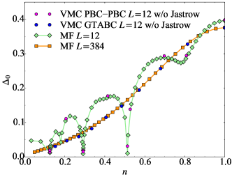
Figure 1: $s$-wave variational parameter $\Delta_{0}$ as a function of $n$ at $U=-2$. Mean-field calculations are performed on $L=12$ and $L=384$ clusters, and VMC calculations are done in GCE without Jastrow correlator on $L=12$ with PBC and TABCs. The error bars in the VMC results are smaller than the symbol sizes.

Before investigating the finite-size effects in correlated systems, it is instructive to study the finite-size effects within the single-particle theory. For this purpose, we treat the negative-$U$ Hubbard model in Eq. (1) within the self-consistent mean-field approximation by decoupling the interaction term into the $s$-wave pairing terms.

Figure 1 shows the $s$-wave superconducting order parameter $\Delta_{0}$ as a function of electron density $n$ ($n=1$ corresponds to the half filling) within the mean-field approximation at $U=-2$ for $L=12$ and $L=384$. We have confirmed that the order parameter does not depend on the system size for $L\geqslant 384$, implying that the results for $L=384$ can be considered very close to the thermodynamic limit. On the other hand, significant size effects, namely the oscillatory dependence on $n$, are observed for $L=12$.

In order to test the accuracy of our VMC calculation, we have reproduced the above results by setting the Jastrow correlator $\mathcal{J}$ in Eq. (4) to be unity, i.e., $v_{i,j}=0$. The VMC calculations are performed for $L=12$, using a single twist or $32\times 32$ twist angles in the whole Brillouin zone. Notice that, the latter case, corresponds, within a mean-field approach, to a single calculation with $L=384$ and PBC. The results obtained by VMC in GCE without Jastrow part are indeed in perfect agreement with those obtained independently by the mean-field calculation.

III.2 $s$-wave variational parameter

The mean-field results do not take into account the correlations between the electrons. The accuracy for treating the electron correlations can be improved by including the Jastrow factor in Eq. (4). Figure 2 shows the superconducting variational parameter $\Delta_{0}$ as a function of electron density $n$ within VMC for $L=12$ and $L=16$ with different boundary conditions and different ensembles. For a fixed system size of $L=12$, the results with a single boundary condition show oscillatory dependencies on $n$, similarly to the ones obtained within the mean-field approximation for $L=12$. With TABCs in both ensembles, the oscillatory dependencies are significantly reduced. By further increasing the system size to $L=16$, a sizable decrease of $\Delta_{0}$ is observed in CE especially for the low-density regime, while the change in GCE is almost negligible, indicating that the GCE shows much smaller size effects.

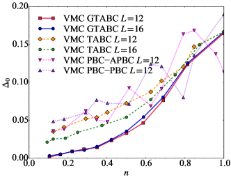
Figure 2: $s$-wave variational parameter $\Delta_{0}$ as a function of $n$ at $U=-2$ calculated by VMC. The system size and boundary conditions used are indicated in the figure. Here, GTABC represents the grand-canonical twist-averaged boundary conditions, TABC the canonical twist-averaged boundary conditions, PBC-APBC stands for PBC in one direction and APBC in the other one, whereas PBC-PBC indicates PBC in both directions. The error bars are smaller than the symbol sizes.

Having confirmed the significant reduction of the finite-size effects, we show in Fig. 3 how the Jastrow correlator affects the magnitude of the optimal variational parameter. By using the same system size of $L=12$ with the same number of twist angles, the Jastrow correlator reduces the magnitude of the $s$-wave variational parameter by more than a factor two for $n=1$. Even when the electron density $n$ is small, the reduction of the variational parameter is not negligible, showing the importance of the inclusion of the electron correlations. Note that, this systematic comparison of the variational wavefunction with and without Jastrow correlator for the entire doping range has been made possible only with GTABCs, because the results with a single boundary condition exhibit oscillatory behaviors both in the mean-field approximation and VMC.

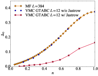
Figure 3: $s$-wave variational parameter $\Delta_{0}$ as a function of $n$ at $U=-2$. The results for mean-field calculations on $L=384$ and VMC on $L=12$ with and without Jastrow correlator in GCE with TABCs are shown. The error bars in the VMC results are smaller than the symbol sizes.

III.3 pairing correlation function

The finite order or variational parameters observed in the mean-field approximation or the VMC for finite-size systems are due to the wavefunction Ansatz that explicitly breaks the U(1) symmetry. In order to compare the VMC results with the ones of the numerically exact AFQMC, it is necessary to study the off-diagonal long-range order by computing superconducting correlation functions. To this purpose we consider the $s$-wave pairing correlation function

$$\phi^{2}(L)=\frac{1}{2N}\sum_{i}\left\langle\Delta_{i}^{\dagger}\Delta_{i+j}+{\rm H.c.}\right\rangle,$$ (14)

where $\Delta_{i}^{\dagger}=c_{i\uparrow}^{{\dagger}}c_{i\downarrow}^{{\dagger}}$ and, $i$ and $i+j$ are sites at the maximum distance allowed by the boundary conditions of the cluster.

Figure 4 shows the calculated pairing correlation functions with VMC for various boundary conditions. As in the case of the variational parameter discussed in the previous section, strong finite-size effects are observed for $L=12$ with a single boundary condition. By increasing the system size to $L=16$, TABCs with CE reduce the oscillatory dependence as a function of $n$, but only with GCE the size effects become almost negligible within the available cluster sizes.

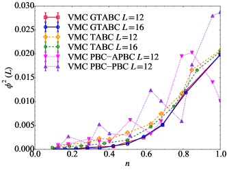
Figure 4: Pairing correlations $\phi^{2}$ as a function of $n$ at $U=-2$ calculated by VMC. The system size and boundary conditions used are indicated in the figure. The notations are the same as those in Fig. 2.

Careful finite-size-scaling analyses for the pairing correlation functions are done for $U=-2,-3,$ and $-4$ at half filling and at quarter filling in Figs. 5 and  6, respectively. We observe that, even at half filling, it is almost impossible to extrapolate the pairing correlations with a single twist since this approximation changes behavior as the system size increases, especially when the value of the $|U|$ is small. Instead, it is clearly evident that the TABCs with GCE represents the best method to deal with finite size effects, also much better than TABCs within CE. In particular, at quarter filling, severe system-size dependencies of the correlation functions are observed, implying that the finite-size scaling with a single twist is almost impossible.

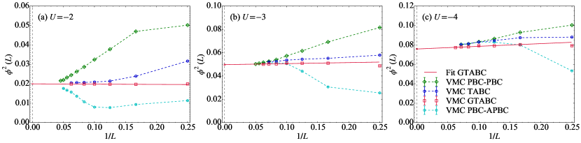
Figure 5: Finite-size-scaling analyses of the pairing correlation $\phi^{2}(L)$ for (a) $U=-2$, (b) $U=-3$, and (c) $U=-4$ by VMC at half filling with different boundary conditions. The solid lines are fits to the GTABC data. The extrapolated values to the thermodynamic limit $\lim_{L\to\infty}\phi^{2}(L)$ are indicated at $1/L=0$ for each panel and correspond to 0.01994(4) for $U=-2$, 0.0497(4) for $U=-3$, and 0.0758(5) for $U=-4$. The notations are the same as in Fig. 2.

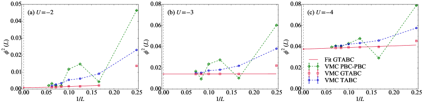
Figure 6: Finite-size-scaling analyses of the pairing correlation $\phi^{2}(L)$ for (a) $U=-2$, (b) $U=-3$, and (c) $U=-4$ by VMC at quarter filling with different boundary conditions. The solid lines are fits to the GTABC data. The extrapolated values to the thermodynamic limit $\lim_{L\to\infty}\phi^{2}(L)$ are indicated at $1/L=0$ for each panel and correspond to 0.00095(25) for $U=-2$, 0.0143(1) for $U=-3$, and 0.0378(4) for $U=-4$. The notations are the same as those in Fig. 2.

Figure 7 shows the pairing correlations obtained with AFQMC for $L=8$ and $L=12$ as well as VMC in GCE on $L=12$. As in the case of VMC, the PBC results show significant size effects, that are reduced significantly by GTABCs also for AFQMC. Close to half filling, within AFQMC, the value of $\phi^{2}$ becomes larger than the corresponding one at half filling, a behavior qualitatively different from the one observed within VMC. This effect has been reported in the early QMC study of the negative-$U$ Hubbard model Scalettar et al. (1989b), and can be attributed to the spin-flop transition in the strong-coupling limit, where the model, at small doping, can be mapped to the Heisenberg model in presence of a small magnetic field (see also Sec. III.4). In this case as soon a non zero magnetic field is present the order parameter “flops” in the xy-plane.

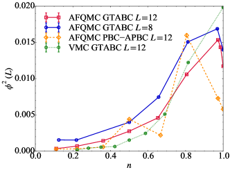
Figure 7: Pairing correlation $\phi^{2}$ as a function of $n$ at $U=-2$ by AFQMC and VMC. The system size and boundary conditions are indicated in the figure. The notations are the same as in Fig. 2.

Despite GTABCs, visible size effects remain in Fig. 7 for the AFQMC case, and we have therefore focused on a few filling values, that we have systematically studied as a function of the system size. We show the finite-size scaling of the pairing correlations at half filling and at quarter filling calculated by AFQMC in Figs. 8 and 9, respectively. As expected from the previous VMC study, also in the case of AFQMC calculations, the TABCs with GCE allows a finite size scaling much better than the one with a single boundary condition. At half filling, the values of $\phi^{2}$ extrapolated to the thermodynamic limit are therefore computed with high accuracy, as shown in Fig. 8.

At quarter filling, the situation is even worse for the single twist approach, and severe system-size dependencies of the correlation functions prevent a systematic extrapolation to the thermodynamic limit. Fortunately this remains possible within TABC approach and controlled extrapolations can be done also for AFQMC calculations. The thermodynamic values of superconducting correlations are therefore computed with high accuracy, as shown in Fig. 9.

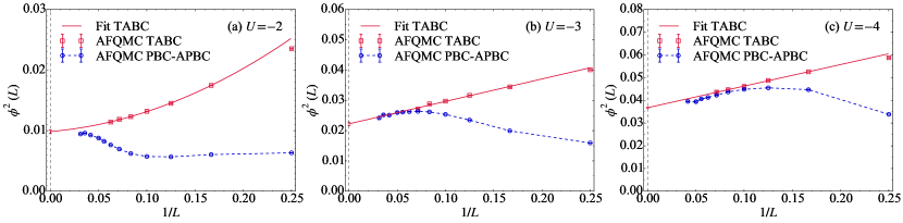
Figure 8: Finite-size-scaling analyses of the pairing correlation $\phi^{2}(L)$ for (a) $U=-2$, (b) $U=-3$, and (c) $U=-4$ by AFQMC at half filling with different boundary conditions. The solid lines are the fit to the TABC data. The TABC extrapolated values to the thermodynamic limit $\lim_{L\to\infty}\phi^{2}(L)$ are indicated at $1/L=0$ for each panel and correspond to 0.0098(3) for $U=-2$, 0.0222(6) for $U=-3$, and 0.0368(2) for $U=-4$. The notations are the same as those in Fig. 2.

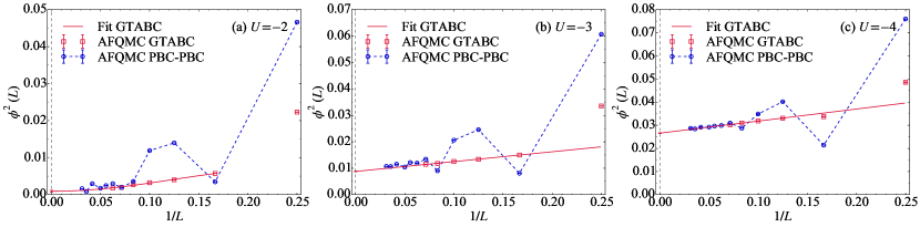
Figure 9: Finite-size-scaling analyses of the pairing correlation $\phi^{2}(L)$ for (a) $U=-2$, (b) $U=-3$, and (c) $U=-4$ by AFQMC at quarter filling with different boundary conditions. The solid lines are the fit to the GTABC data. The GTABC extrapolated values to the thermodynamic limit $\lim_{L\to\infty}\phi^{2}(L)$ are indicated at $1/L=0$ for each panel and correspond to 0.0009(3) for $U=-2$, 0.0088(1) for $U=-3$, and 0.0266(2) for $U=-4$. The notations are the same as those in Fig. 2.

III.4 Attractive-repulsive mapping and order parameters

The negative-$U$ Hubbard model can be mapped to the positive-$U$ Hubbard model with the particle-hole transformation Shiba (1972)

$$\tilde{c}_{i\uparrow} :=c_{i\uparrow},$$ (15)

$$\tilde{c}_{i\downarrow} :=(-1)^{x_{i}+y_{i}}c_{i\downarrow}^{\dagger}.$$ (16)

This mapping allows us to compare the results of the pairing correlation function $\phi^{2}(L)$ with those of the transverse spin-spin correlation function in the positive-$U$ Hubbard model. Indeed, in terms of the newly defined operators $\tilde{c}_{i\sigma}$, $\tilde{c}_{i\sigma}^{\dagger}$ and $\tilde{n}_{i\sigma}=\tilde{c}_{i\sigma}^{\dagger}\tilde{c}_{i\sigma}$, the Hamiltonian changes, up to a constant, to:

$$H = -t\sum_{\langle i,j\rangle,\sigma}\left(\tilde{c}^{\dagger}_{i\sigma}\tilde{c}^{\phantom{\dagger}}_{j\sigma}+{\rm H.c.}\right)+|U|\sum_{i}\tilde{n}_{i\uparrow}\tilde{n}_{i\downarrow}$$ (17)

$$- \sum_{i}\left[(\mu-U)\tilde{n}_{i\uparrow}-\mu\tilde{n}_{i\downarrow}\right],$$

whereas $\phi^{2}(L)$ can be written as the transverse spin-spin correlation function

$$M^{2}_{xy}(L) = \frac{1}{2N}\sum_{i}(-1)^{x_{j}+y_{j}}\left\langle S_{i}^{+}S_{i+j}^{-}+{\rm H.c.}\right\rangle$$ (18)

$$= \frac{1}{N}\sum_{i}(-1)^{x_{j}+y_{j}}\left\langle S_{i}^{x}S_{i+j}^{x}+S_{i}^{y}S_{i+j}^{y}\right\rangle,$$

where $S_{i}^{+}=\tilde{c}_{i\uparrow}^{\dagger}\tilde{c}_{i\downarrow}$, $S_{i}^{-}={(S_{i}^{+})}^{\dagger}$, $S_{i}^{x}=(S_{i}^{+}+S_{i}^{-})/2$, and $S_{i}^{y}=(S_{i}^{+}-S_{i}^{-})/2{\rm i}$. Similarly, the charge-charge correlations in the negative-$U$ Hubbard model can be mapped to the longitudinal spin-spin correlations in the positive-$U$ Hubbard model. In the present study, however, the charge-charge correlations are not considered as they will not dominate over the pairing correlations for large distances away from the half filling.

Since the negative-$U$ Hubbard model with $\mu=U/2$ (the half-filled case) corresponds to the positive-$U$ Hubbard model with zero magnetic field, the SU(2) symmetric staggered magnetization $M_{0}$ in the thermodynamic limit can be estimated from $M_{xy}(L)$ through the relation

$$M_{0}=\sqrt{\frac{3}{2}\lim_{L\to\infty}M^{2}_{xy}(L)},$$ (19)

where the factor $3/2$ within the square root is included to take into account the contribution from the longitudinal spin-spin correlation which is not present in $M_{xy}^{2}(L)$. The estimated values of $M_{0}$ are reported in Table 1. For $|U|=2$ and $4$, these values are in agreement with a recent study Qin et al. (2016) and, for $|U|=2$, also with a previous work Sorella (2015) by one of us. On the other hand an earlier work LeBlanc et al. (2015) reported a too small value of $M_{0}$ for $|U|=2t$, that was however affected by an error in the extrapolation to the thermodynamic limit Qin et al. (2016).

At quarter filling, the CDW order disappears and we are left to study only the $s$-wave order parameter defined as

$$\Phi_{s}=\sqrt{\lim_{L\to\infty}\phi^{2}(L)}.$$ (20)

The estimated values of $\Phi_{s}$ from the extrapolated values of $\phi^{2}(L)$ are reported in Table 2.

In order to test the accuracy of the variational wave function in the thermodynamic limit, we have also compared the VMC estimates of the ground state energies with the AFQMC ones in Table 3 and Table 4 at half filling and at quarter filling, respectively. The energies obtained via AFQMC in the present study are in agreement with the exact energies of previous works. It is worth mentioning that VMC energies are providing quite good upper bounds to the exact energies, especially in the weak-coupling regime.

Table 1: Comparison of the $s$-wave superconducting (antiferromagnetic) order parameter $M_{0}$ defined in Eq. (19) for the negative (positive)-$U$ Hubbard model at half filling ($n=1$). For the VMC case we have not included the factor $\sqrt{3\over 2}$, see discussion in the conclusions. The number in each parenthesis in this work indicates the uncertainty due to the extrapolation to the thermodynamic limit. The AFQMC simulations in Ref. Sorella (2015) are performed with the modified-boundary conditions, while in Refs Qin et al. (2016) and LeBlanc et al. (2015) with the TABCs method. DMET stands for density-matrix-embedding theory, and MF for the standard BCS mean-field theory.

$n=1$
$|U|/t$	2	3	4
MF	0.1881	0.2830	0.3453
VMC (this work)	0.1412(1)	0.2230(6)	0.2752(6)
AFQMC (this work)	0.122(1)	0.183(2)	0.2347(4)
AFQMC Sorella (2015)	0.120(5)	–	–
AFQMC Qin et al. (2016)	0.119(4)	–	0.236(1)
AFQMC LeBlanc et al. (2015)	0.094(4)	–	0.236(1)
DMET LeBlanc et al. (2015)	0.133(5)	–	0.252(9)

Table 2: Comparison of the $s$-wave superconducting order parameter $\Phi_{s}$ defined in Eq. (20) for the negative-$U$ Hubbard model at quarter filling ($n=0.5$). The number in each parenthesis in this work indicates the uncertainty due to the extrapolation to the thermodynamic limit.

$n=0.5$
$|U|/t$	2	3	4
VMC (this work)	0.031(4)	0.1196(6)	0.194(1)
AFQMC (this work)	0.030(4)	0.094(1)	0.163(1)

Table 3: Comparison of the ground state energies for the negative (positive)-$U$ Hubbard model at half filling ($n=1$). The number in each parenthesis in this work indicates the uncertainty due to the extrapolation to the thermodynamic limit.

$n=1$
$|U|/t$	2	3	4
VMC (this work)	-2.16848(1)	-2.49007(1)	-2.84769(5)
AFQMC (this work)	-2.1755(3)	-2.5014(3)	-2.86016(9)
AFQMC Sorella (2015)	-2.175469(92)	-2.501412(52)	–
AFQMC Qin et al. (2016)	-2.1760(2)	–	-2.8603(2)
AFQMC LeBlanc et al. (2015)	-2.1763(2)	–	-2.8603(2)
DMET LeBlanc et al. (2015)	-2.1764(3)	–	-2.8604(3)

Table 4: Comparison of the ground state energies for the negative-$U$ Hubbard model at quarter filling ($n=0.5$). The number in each parenthesis in this work indicates the uncertainty due to the extrapolation to the thermodynamic limit.

$n=0.5$
$|U|/t$	2	3	4
VMC (this work)	-1.4615(2)	-1.55820(6)	-1.68016(4)
AFQMC (this work)	-1.4652(5)	-1.5669(5)	-1.6920(2)

IV Conclusions and discussions

To conclude, finite-size effects on the $s$-wave order parameter and pairing correlation functions have been studied in details for the negative-$U$ Hubbard model with VMC and AFQMC methods. GTABCs reduce systematically the finite size effects and provide smooth extrapolation to the thermodynamic limit. This has enabled us to obtain well converged results on energy and order parameter for several values of $U/t$ and doping, and to study very efficiently the physical properties in the thermodynamic limits of our Jastrow correlated wavefunction as a function of doping. Indeed, we have shown that the Jastrow correlator in VMC significantly reduces the magnitude of the $s$-wave variational parameter in the entire doping range, already at $U=-2$.

We have also presented the comparison of the pairing correlation functions obtained by VMC and by the numerically exact AFQMC. In this case VMC is in good agreement with AFQMC for finite doping. At half filling, there exists a pseudo-SU(2) symmetry defined by the SU(2) rotations in spin space applied to the Hamiltonian after the particle-hole transformation in Eq. (15), that remains therefore invariant and commuting with the pseudo spin operators [the spin operators after the particle-hole transformation of Eq. (15)]. This symmetry is clearly accidental, as is no longer satisfied by the inclusion of a tiny next-nearest-neighbor hopping $t^{\prime}$ Otsuka et al. . Since our variational wavefunction breaks this accidental pseudo-SU(2) symmetry the agreement between the VMC and the necessarily symmetrical (as the exact ground state in any finite lattice is a singlet after particle-hole transformation Lieb (1989)) AFQMC in this case is not very good just because in the VMC the order is only in one of the possible directions of a three-component order parameter. For this reason, when comparing VMC and AFQMC in Table 1, we have not included in the VMC entries the factor $\sqrt{3/2}$ implied by the definition of $M_{0}$ in Eq. (19), as we have verified that, within VMC, the order is in the $xy$ plane, because the CDW order, corresponding, in the positive-$U$ language, to the $z$ component of the antiferromagnetic order-parameter, is always negligible. This consideration explains also why the spin-flop transition observed in AFQMC – $M_{xy}$ jumps to a larger value as soon as we depart from half-filling – is not present in VMC, because, as shown in Fig. 7, $M_{xy}$ appears a smooth and monotonically decreasing function of the doping.

Apart for symmetry considerations, that can be restored by standard symmetry projection techniquesTahara and Imada (2008); Rodríguez-Guzmán et al. (2012), our wavefunction can be also improved, for example, by taking into account the backflow correlations Holzmann et al. (2003), as it was done in the positive-$U$ Hubbard model Tocchio et al. (2008, 2011).

The method for reducing finite-size effects, developed in this paper, is applicable for any correlated lattice model. The calculation in GCE will be particularly useful for investigating the doping dependence of the $d$-wave superconductivity in the positive-$U$ Hubbard model with parameters relevant for cuprates. Furthermore, the reduction of the order parameter in the entire doping range due to the Jastrow factor suggests that the electron-correlation are not be negligible even for weakly attracting fermions in the low-electron-density regime. This implies that the method will be also promising for studying the ground-state properties of dilute electron systems. Such systems may include TiSe₂ in the series of transition metal dichalcogenides Monney et al. (2010); Rossnagel (2011); Watanabe et al. (2015); Kaneko et al. (2018), where its electronic state is in vicinity of the semimetal-semiconductor transition and considered to be a candidate of excitonic insulators, in which coherent electron-hole pairs are formed and condensate spontaneously Jérome et al. (1967); Halperin and Rice (1968).