A time-delay model for molecular gas flow into vacuum

Abstract

Flow of molecular gas into a complex vacuum system is investigated by a lumped parameter model to estimate the time evolution of gas pressure $p_{g}$, which for the first time takes into account the realistic effect of time-delay arising due to multiple reasons such as valve response, pumping and transport of gas, conductance of the pipe network, etc. The net effect of all such delays taken together into a single (constant) delay term gives rise to a scalar delay differential equation (DDE). Analytical solutions of a linear DDE in presence of external forcing due to the (pulsed) injection of gas and outgassing from a stainless steel (SS) wall are then derived using the Laplace transform method, where the transcendental characteristic equation is approximated by means of rational transfer functions such as diagonal Padé approximation. A good agreement is obtained with the numerical results and it is shown from these solutions that a reasonably good match with experimental results is obtained only in the presence of a nonzero time-delay. An attempt is also made to simplify the DDE into an ordinary differential equation (ODE) by using a low-order Taylor series expansion of the time-delay term. A singular perturbation method is used to solve the resultant initial value problem (IVP) type second-order ODE. It is found that unlike the Laplace transform method, the ODE closely approximates the DDE only if the delay is small. Emergence of stable periodic oscillations in $p_{g}$, as a generic supercritical Hopf bifurcation, if time-delay exceeds a critical value is then established by numerical and Poincaré-Lindstedt method.

I Introduction and motivation

It is now widely agreed that there exist a number of gas flow and pressure measurements that are useful for an efficient operation of many complex systems such as, airflows in ventilation systems, helium transport in cryogenic devices, gas pipelines, fabrication processes in microelectronics, magnetic confinement devices such as tokamaks and stellarators, etc. It is instructive to note that the parameter of pressure is also used as an indicator of the quality of vacuum present in some of these systems. However, the nature of gas flow changes with the gas pressure and so its description is decided by the value of the Knudsen number ${\rm{Kn}}=\lambda/d$ ($\lambda$ is the mean free path and $d$ is characteristic size of the cross section through which the gas is flowing), dividing the flow regions into three main categories, viscous, intermediate, and molecular. Although a detailed dynamic model based on fluid or kinetic modeling, taking into account several (actual) flow interconnections in a complex geometry would be ideally desirable, it may not turn out to be easy and fast enough for any real-time objectives. For example, eventhough molecular flow is theoretically the best understood of any flow type,J.F. O’Hanlon (2003) an accurate estimation of conductances would require to take into account beaming and exit/entrance corrections, preferably by the Monte Carlo method. Instead, one could utilise space-averaged models that substantially reduce the computational load needed to describe these extensively interconnected gas flow networks. This paper presents one such model for transient pressure behaviour, and since the experimental results needed for its justification have been obtained on a device with a largely molecular flow (${\rm{Kn}}>1$), our theoretical model likewise assumes that the flow is molecular throughout the network. This implies that the flow is predominantly determined by gas-wall collisions, with diffuse reflection at most wall surfaces.J.F. O’Hanlon (2003) A model encompassing the entire range of flow, from viscous to molecular, is beyond the scope of this paper.

Many analytical and numerical models exist for molecular flow conditions. B.R.F. Kendall and R.E. Pulfrey (1969); K.M. Welch (1973); Kanazawa (1988); Ohta, Yoshimura, and Hirano (1983); S.R. Wilson (1987) Most of these studies utilise the close correspondence between a molecular flow and an electrical circuit. Vacuum conductances are constant and not a function of pressure in this flow regime, and thus analogous to electric conductances. It is further assumed that conductance through each segment of the network is the same as a stand-alone component, and hence a lumped-sum value can be used to calculate the network conductance.J.A. Theil (1994) However, in order to make these simple lumped parameter models more realistic, we have included the important yet neglected role played by time-delay, which appears to be an inherent and non-negligible factor in a large complex system. This time lag arising mainly out of the conductances of pipes of assorted shapes and sizes connected in series and parallel, is analogous to that of having many serial resistors and parallel capacitors in an electrical circuit.Poschenrieder, Venus, and the ASDEX-Team (1982) Thus, these simpler zero-dimensional (0D) DDE models could then provide a promising alternative to the sophisticated yet cumbersome partial differential equation (PDE) based fluid/kinetic models, especially to quickly estimate some global system parameters such as pumping speeds, overall conductance of the pipe network, magnitude of outgassing/wall pumping, etc.

As opposed to ODEs, DDEs belong to a class of functional differential equations (FDEs) which are infinite-dimensional, since the function that specifies the initial value requires an infinite number of points to specify it. Consequently, DDEs can have oscillatory and chaotic dynamical behaviours. Beuter et al. (2003) In general, these DDEs arise when modelling processes whose rate of change of state at any moment of time $t$ is determined not only by the present state, but also by past states. Kolmanovskii and Myshkis (1999) The use of delay equations to take into account the transport phenomena in a network of pipes can be advantageous, since there is no need to analyze the complex spatial details of the transmission and transport. However, the results obtained on the basis of this model are only qualitative, because of the approximate nature of the hypothesis as well as the low reliability of the empirical constants used when deriving these equations. A few questions concerning the influence of delays can also be raised, such as (i) can they destabilize an otherwise stable linear system, (ii) can they stabilize an otherwise unstable system, or (iii) is switching from stability to instablility and back to stability possible, etc.K.L. Cooke and Grossman (1982); Gopalsamy (1992) Nevertheless, DDEs have now gained a wide usage in modelling diverse fields ranging from population biology, epidemiology, nonlinear optics, economics, control of mechanical systems, etc. Erneux (2009)

The paper is organized as follows: A detailed outline of our simple and fast global 0D model is presented in Sec. II. To validate our theoretical model with an experimental result, we have chosen to apply it to a magnetic confinement device called tokamak.Wesson (2011) The standard method to initiate plasma in these machines is to first evacuate the confinement vessel to a background (base) pressure of $\lesssim 10^{-7}$ Torr and then open a gas reservoir valve, usually at a single toroidal location, for a short duration to flow in the working gas (hydrogen or deuterium) so that a typical (maximum) pre-fill neutral gas pressure $p_{g}$ of $\sim 10^{-4}$ Torr is established in the chamber, which is then ionized by applying a toroidal electric field $E$ via transformer action from a central solenoid. Note that the vessel remains under continuous pumping throughout. Our theoretical model includes for the first time the effect of time-delay to help describe the observed time variation of $p_{g}$. In Section III we first present an analytical solution of our DDE model using the Laplace transform method wherein the time-delay term leads to a transcendental characteristic equation, which is solved by using the diagonal Padé approximation. We then attempt to simplify the infinite-dimensional DDE into a finite-dimensional equation by using a low-order Taylor series expansion to approximate the delay term. A singular perturbation methodP.V. Kokotović, R.E. O’Malley, Jr., and Sannuti (1976); P.V. Kokotović (1984) is to used solve the resultant IVP type second-order ODE. Next, we examine the possibility of a Hopf type bifurcation which can occur in phase spaces of any nonlinear system with dimension $n\geq 2$.S.H. Strogatz (1994) Apart from a numerical solution, the Poincaré-Lindstedt method is used to analytically figure out whether the limit cycle oscillations are stable (supercritical) or unstable (subcritical). Section IV contains the quantitative validation of our model derived pre-fill pressure. To do so we first solve the DDE numerically using ADITYA tokamak parameters and then compare these solutions with the above mentioned analytical and experimentally obtained results. Section V is devoted to discussion, and conclusions are summarized.

II Model

Usually a detailed treatment of gas flow in tubes has been carried out either with Clausing-type integral equations or by statistical computations based on Monte Carlo methods which are particularly well suited for complex shapes and systems of baffles, traps, etc. Steckelmacher (1986) In the present paper we have however analyzed the response of an evacuated vessel, SS type $304$ in particular, to sources and sinks by the following 0D equation for the flow of hydrogen gas. Assuming that the velocities are randomized and the concept of scalar pressure is valid,

$$\frac{d}{dt}\left(p_{g}V\right)=Q-Sp_{g}$$ (1)

where $p_{g}$ is the neutral gas pressure, $V$ is volume of the vessel being pumped out, throughput $Q$ includes all significant sources of gas, and $S$ is the effective pumping speed delivered by all significant sinks. Now, it is known that there exist several other types of sources such as normal outgassing, permeation, leaks, etc, as well as sinks in addition to the system pumps, such as wall pumping and gauge pumping, etc. The process of co-deposition, hydrogen trapping, as well as standard surface cleaning techniques such as glow discharge cleaning (GDC) facilitate hydrogen loading. Typically, an outgassing model involves diffusion of dissolved hydrogen atoms through the bulk material to be adsorbed at surface sites and recombination of two adsorbed particles which then desorb as hydrogen molecule from the surface.P.A. Redhead, J.P. Hobson, and E.V. Kornelson (1993) However, these models do not consider the influence of hydrogen traps which may comprise less than $0.1\%$ of all lattice sites, but can hold almost all of the hydrogen.R.F. Berg (2014) It is thus amply clear that a precise quantitative modelling of the wall sources and sinks is nontrivial. However, to qualitatively account for the generic outgassing/wall pumping of an SS surface in high vacuum, we simply introduce an additional feedback term proportional to the instantaneous gas pressure in Eq. (1). In addition we have also considered gas input through a piezoelectric valve of a known throughput and whose voltage waveforms are feedforward programmed to fill the tokamak to a preset (desired) pressure.

On the other hand, the effects of extensive pipe network and interconnections such as traps, baffles, and ducts which impede the flow of gas and reduce the pumping effect of the system have been lumped and approximated through the overall value of the conductance parameter $C$. Interestingly, the conductance $C$ of a pipe depends on whether the gas flow is molecular, intermediate, or viscous. Thus the effective pumping speed $S$ obtained in a chamber, connected by the effective conductance $C$ to a pump having a pumping speed $S_{\rm{p}}$ as,Roth (1989)

$$S=\frac{CS_{\rm{p}}}{C+S_{\rm{p}}}$$ (2)

Note that a solution of Eq. (1) will depend on the location where $p_{g}$ is measured. We have assumed that heat transfer effects are negligible and the gas quickly adjusts to the temperature of the vessel or pumping ducts, and is therefore taken as constant. Fortuitously, it also helps in direct comparision with the experimental values since the Bayard-Alpert type hot cathode ionization gauge (BA-IG) typically deployed under such vacuum conditions in principle measure densities and not pressure.

Note that Eq. (1) is valid if we assume a continuous, instantaneous and perfect mixing throughout the vacuum vessel. But, a realistic consideration would yield that the pressure of the gas being registered in a gauge at time $t$ will equal the average pressure in the vessel at some earlier instant, say $t-\tau$. Here for simplicity we have assumed that the time-delay parameter $\tau$ represents a sum of all delays present in the system and is therefore taken to be a single positive constant.

Combining all of these with the equation of state $p_{g}V=NkT$, where $N=nV$, $n$ and $T$ are gas density and (constant) gas temperature, respectively, we can now reformulate Eq. (1) as the following DDE,

$$\begin{split}\frac{dN(t)}{dt}=Q_{0}\exp\left[-\left(\frac{t-t_{0}}{\delta}\right)^{2}\right]+aN(t)-\alpha N(t-\tau)\end{split}$$ (3)

where, $Q_{0}=Q/kT$ and $\alpha=S/V$. Eq. (1) now describes the time variation of the number of molecules $N(t)$ (of the working gas) contained in the vacuum vessel at time $t$. Here, for analytical tractability as well as closeness to actual physical system, we have used a Gaussian function to describe the piezoelectric valve behaviour and $t_{0}\gg\delta>0$ is assumed here. The parameters $Q_{0}$, $a$, and $\alpha$ are related to the maximum throughput of the valve, outgassing ($a>0$) or wall pumping ($a<0$) rate, and pumping speed, respectively, and for simplicity are taken to be constants. Interestingly, the presence of a delayed negative feedback term in Eq. (3) stabilizes an otherwise asymptotically unstable system provided, Gopalsamy (1992)

$$\alpha>\left(a^{2}+\alpha^{2}\tau+a\alpha\tau\right)$$ (4)

In order to obtain a unique solution of Eq. (3), we have to now specify an initial condition in the form of a function $\theta$ for a period of time equal to the duration of the time-delay and then seek a function $N$ such that $N(t)=\theta(t)$ for $-\tau\leq t\leq 0$, and $N$ satisfies Eq. (3) for $t\geq 0$. In the present case we shall take $\theta(t)\equiv N_{0}$, a positive constant associated with the base pressure values.

Incidentally, Eq. (3) can also be derived as the linearized form of a generalized delay-logistic equation of the typeGopalsamy (1992)

$$\frac{dN(t)}{dt}=N(t)\left[a_{1}-a_{2}N(t-\tau)+a_{3}N(t)\right]$$ (5)

and have the asymptotic behaviour

$$\lim_{t\to\infty}N(t)=N_{0},\hskip 7.22743ptN_{0}=\frac{a_{1}}{a_{2}-a_{3}}$$

Now, letting $N(t)=N_{0}+x(t)$ yields the following variational equation

$$\frac{dx(t)}{dt}=ax(t)-\alpha x(t-\tau)+f\left(x(t),x(t-\tau)\right)$$ (6)

where

$$a=a_{3}N_{0},\hskip 10.84006pt\alpha=a_{2}N_{0}$$

$$f\left(x(t),x(t-\tau)\right)=\frac{1}{N_{0}}\left[ax^{2}(t)-\alpha x(t)x(t-\tau)\right]$$

Linear approximation of Eq. (6) thus nicely approximates our DDE model given by Eq. (3) sans the external gas input through a valve. Further, it will be shown that these equations admit Hopf-type bifurcation to a periodic solution and a constant steady state becomes unstable for a critical value of $\tau$.Gopalsamy (1992) Note that in absence of external forcing, for autonomous monotone feedback systems with delay, a Poincaré-Bendixson type theorem implies that bound solutions converge either to an equilibrium or to a periodic orbit, and thus, chaotic trajectories are not possible.J. Mallet-Paret and Sell (1996)

III Analytical Results

Although Eq. (3) can be solved analytically by the ‘method of steps’, Driver (1977) the calculations become unwieldy if the delay $\tau$ is small relative to the interval on which it is desired to determine the solution. L.E. El’sgol’ts and S.B. Norkin (1973) Hence, we present two different analytical methods for obtaining the solution of the DDE, which are later compared with numerical and experimental results. For studying the possibility of Hopf bifurcation we have resorted to the standard Poincaré-Lindstedt perturbation method, which is then verified by numerical computation.

III.1 Laplace transform

In this subsection we shall present another analytical method to solve a nonhomogeneous DDE like Eq. (3) i.e., by means of the Laplace transform. Thus Eq. (1) takes the form

$$\begin{split}\left(s-a+\alpha e^{-s\tau}\right)\int_{0}^{\infty}e^{-st}N(t)dt=\frac{N_{0}}{s}\left(s-\alpha+\alpha e^{-s\tau}\right)\\ +Q_{0}\int_{0}^{\infty}\exp\left[-st-\left(\frac{t-t_{0}}{\delta}\right)^{2}\right]dt\end{split}$$ (7)

Now assuming that an inversion can be performed, the solution of Eq. (1) can be expressed by means of a contour integral taken along the vertical line joining the points $b-iT$ and $b+iT$ in the complex plane, Bellman and K.L. Cooke (1963) so

$$\begin{split}N(t)=\lim_{T\to\infty}\frac{1}{2\pi i}\int_{b-iT}^{b+iT}e^{st}\Biggl{\{}\frac{N_{0}}{s}\Bigl{[}1-h^{-1}(s)\left(\alpha-a\right)\Bigr{]}\\ +Q_{0}h^{-1}(s)\int_{0}^{T}\exp\left[-st_{1}-\left(\frac{t_{1}-t_{0}}{\delta}\right)^{2}\right]dt_{1}\Biggr{\}}ds\end{split}$$ (8)

where the (transcendental) function $h(s)=s-a+\alpha e^{-s\tau}$ is called the characteristic function, and the roots of the characteristic equation $h(s)=0$ are called the characteristic roots. Now to evaluate the integral on right side of Eq. (8), one needs to know all the zeros of this exponential polynomial in order to calculate the residues contribution. However, although there are, in general, infinitely many characteristic roots of a transcendental equation, according to complex variables theory, since $h(s)$ is an entire function, the characteristic equation cannot have an infinite number of zeros within any compact set $|s|\leq R$, for any finite $R>0$. Therefore, most of the system’s poles go to infinity. Gu, V.L. Kharitonov, and Chen (2003)

Nevertheless, to further reduce the complexity of locating the zeros of the characteristic functions in the complex plane, model order reduction by treating an infinite-dimensional system like a finite-dimensional one have been proposed. Here the main motivation is to approximate delays by means of rational transfer functions and generally involves the truncation of some infinite series, which can be achieved via the following approximation: J.-P. Richard (2003)

$$e^{-\tau s}\approx\frac{p(-\tau s)}{p(\tau s)}$$

where $p\in\mathbb{R}[\tau s]$ is an appropriate polynomial without any zero in the right half-plane Re $s\geq 0$, such as the diagonal Padé approximation,M.F. Reusch et al. (1988) Laguerre-Fourier and Kautz series, P.M. Mäkilä and J.R. Partington (1999) etc. In this paper we shall use a diagonal Padé approximant of order $n\geq 3$, as they are known to have optimal accuracy and the odd-order method also preserves positivity. M.F. Reusch et al. (1988) Thus we replace the exponential in the characteristic equation by

$$e^{z}=\frac{P_{n}(z)}{P_{n}(-z)},\hskip 9.39545ptP_{n}(z)=\sum_{m=0}^{n}\frac{n!\,(2n-m)!}{(2n)!\,m!\,(n-m)!}z^{m}$$ (9)

We then use Eq. (9) to obtain the dominant roots of the characteristic equation, as those closest to the imaginary axis correspond to slowly decaying components which generate the long term response, whereas, far away poles correspond to components that decay rapidly. To gain qualitative insights into the response characteristics of the time-delay system, we shall plot the location of the poles and zeros of the transfer function $H(s)\equiv h^{-1}(s)$ in the complex $s$-plane, since it is well known that the transfer function poles are the roots of the characteristic equation.

III.2 Singular perturbation

Since DDEs, as demonstrated above, are particularly difficult to study analytically,Bellman and K.L. Cooke (1963) attempts have also been made to approximate them by using a low-order Taylor series expansion of the time-delay term and ignoring high order derivatives.Mazanov and K.P. Tognetti (1974) Here, assuming the (constant) delay $\tau$ to be small, we replace $N(t-\tau)$ with the first few terms of a Taylor series such that Eq. (3) becomes,

$$\begin{split}\varepsilon^{2}\frac{d^{2}N(t)}{dt^{2}}+\frac{\alpha}{2}\left(1-2\varepsilon\right)\frac{dN(t)}{dt}+\frac{\alpha}{2}\left(\alpha-a\right)N(t)=\\ \left(\frac{\alpha}{2}\right)Q_{0}\exp\left[-\left(\frac{t-t_{0}}{\delta}\right)^{2}\right]\end{split}$$ (10)

where $\varepsilon=\alpha\tau/2$ and subject to the initial conditions $N(0)=N_{0}$ and $dN(0)/dt=0$.

Since the highest derivative of our differential equation (10) is multiplied by a small parameter $\varepsilon^{2}$ which lowers the order of the ODE when $\varepsilon=0$, it represents a singular perturbation problem. Such problems are typically characterized by a boundary-layer which is a narrow region where the solution of a differential equation changes rapidly. Although the method of matched asymptotic expansions has been successfully applied to numerous problems which involve singular perturbations, they are usually of the boundary value type Bender and Orszag (1999); A.H. Nayfeh (2004), whereas here we shall use a slightly different perturbative concept to obtain the solution $N(t)$ of the IVP given by Eq. (10). Such concepts have been very helpful in control and systems theory and optimization of dynamic systems. P.V. Kokotović, R.E. O’Malley, Jr., and Sannuti (1976); P.V. Kokotović (1984)

It is known that in response to an external stimuli, singular perturbations cause a multi-time-scale behaviour of dynamic systems characterized by the presence of both slow and fast transients. Note that this decomposition coincides with the asymptotic expansions into reduced (‘outer’) and boundary-layer (‘inner’) regions. Typically, the reduced model represents the slowest (average) phenomena which are usually dominant, while the boundary-layer models evolve in faster time scales and represent deviations from the predicted slow behaviour. P.V. Kokotović (1984) This separation of time scales also eliminates stiffness difficulties. We shall assume that the solution of Eq. (10) is slowly varying except in an isolated section closer to $t=t_{0}$, and away from this only boundary-layer the behaviour of $N(t)$ is characterized by the absence of rapid variation.

As a step towards a ‘reduced-order model’, we rewrite Eq. (10) as a linear system,

$$\frac{dN}{dt}=z$$ (11a)

$$\varepsilon^{2}\frac{dz}{dt}=-\frac{\alpha}{2}\left(1-2\varepsilon\right)z-\frac{\alpha}{2}\left(\alpha-a\right)N$$

$$+\left(\frac{\alpha}{2}\right)Q_{0}\exp\left[-\left(\frac{t-t_{0}}{\delta}\right)^{2}\right]$$ (11b)

subject to the initial values $N(0)=N_{0}$ and $z(0)=0$. On setting $\varepsilon=0$, Eq. (11b) degenerates into an algebraic equation whose root $\bar{z}$ (bar is used to indicate the variables for whom $\varepsilon=0$) is then substituted into Eq. (11a). Its solution $\bar{N}(t)$ is then evaluated, while constrained to the prescribed initial condition $\bar{N}(0)=N_{0}$, thus yielding the ‘reduced model’. We then input $\bar{N}(t)$ back into the root equation to get $\bar{z}(t)$. Now, to understand when these reduced solution $\bar{N}$, $\bar{z}$ approximate the original solution $N$, $z$, respectively, we first estimate the error $z-\bar{z}$ by defining a boundary-layer correction P.V. Kokotović, R.E. O’Malley, Jr., and Sannuti (1976)

$$\eta=z+\beta_{1}N$$ (12)

where $\beta_{1}=\left(\alpha-a\right)/\left(1-2\varepsilon\right)+m_{1}\varepsilon^{2}$ and $m_{1}$ is chosen such that substitution of Eq. (12) into Eqs. (11a)-(11b) separates out the $\eta$-subsystem as

$$\frac{dN}{dt}=-\beta_{1}N+\eta$$ (13a)

$$\frac{d\eta}{d\tau}+\beta_{2}\eta=\left(\frac{\alpha}{2}\right)Q_{0}\exp\left[-\varepsilon^{4}\left(\frac{\tau-\tau_{0}}{\delta}\right)^{2}\right]$$ (13b)

where $\beta_{2}=\alpha\left(1-2\varepsilon\right)/2-\beta_{1}\varepsilon^{2}$. Eq. (13b) is the ‘fast’ part of Eqs. (11a)-(11b), and $\tau=t/\varepsilon^{2}$ is the ‘stretched time scale’ defined for all $\varepsilon\geq 0$. The solution of the ‘fast’ subsystem Eq. (13b) with the initial condition $\eta(0)$ obtained from Eq. (12) is then input to the ‘slow’ subsystem given by Eq. (13a). Integration of the resultant ODE then gives,

$$N(t)=\left[\frac{N_{0}}{\beta_{1}-\beta_{2}/\varepsilon^{2}}\right]\times$$

$$\left[\beta_{1}\exp\left(-\beta_{2}t/\varepsilon^{2}\right)-\frac{\beta_{2}}{\varepsilon^{2}}\exp\left(-\beta_{1}t\right)\right]+$$

$$\left(\frac{\alpha Q_{0}\sqrt{\pi}\delta}{4\varepsilon^{2}}\right)\left(\frac{1}{\beta_{1}-\beta_{2}/\varepsilon^{2}}\right)\left\{\exp\left[\frac{\beta_{2}^{2}\delta^{2}}{4\varepsilon^{4}}+\frac{\beta_{2}\left(t_{0}-t\right)}{\varepsilon^{2}}\right]\times\right.$$

$$\left.\left[\operatorname{erf}\left(\frac{\beta_{2}\delta^{2}/\varepsilon^{2}+2t_{0}}{2\delta}\right)-\operatorname{erf}\left(\frac{\beta_{2}\delta^{2}/\varepsilon^{2}+2t_{0}-2t}{2\delta}\right)\right]+\right.$$

$$\left.\exp\left[\frac{\beta_{1}^{2}\delta^{2}}{4}+\beta_{1}\left(t_{0}-t\right)\right]\times\right.$$

$$\left.\left[\operatorname{erf}\left(\frac{\beta_{1}\delta^{2}+2t_{0}-2t}{2\delta}\right)-\operatorname{erf}\left(\frac{\beta_{1}\delta^{2}+2t_{0}}{2\delta}\right)\right]\right\}$$ (14)

where the condition $N(0)=N_{0}$ is used to evaluate the constant of integration. It is easily verified that for $\tau=0$ the solution given by Eq. (14) reduces to that obtained from Eq. (3) in case of zero time delay.

III.3 Hopf bifurcation

It is well known that if all the poles of a characteristic equation turn out to have negative real parts, then from the stability standpoint the system is asymptotically stable as all solutions decay to zero under an arbitrary initial condition. In case of ODEs, a stability analysis based on the characteristic equation is almost trivial due to the availability of the Routh-Hurwitz criterion.Gopalsamy (1992) In our case if we let $z=s\tau$, $p=a\tau$, $q=-\alpha\tau$, then the characteristic equation $h(s)=0$ (refer III.1) is equivalent to

$$pe^{z}+q-ze^{z}=0$$ (15)

A necessary and sufficient condition in order that all roots of Eq. (15) have negative real parts is that K.L. Cooke and Grossman (1982)

1. $p<1$ and

2. $p<-q<\left(\theta^{2}+p^{2}\right)^{1/2}$

where $\theta$ is the unique root of $\theta=p\tan\theta$, $0<\theta<\pi$. Now, if $\alpha>0$, these stability conditions reduce to K.L. Cooke and Grossman (1982)

$$a\tau<1,\hskip 9.39545pta<|\alpha|<|a^{2}+\left(\theta/\tau\right)^{2}|^{1/2}$$ (16)

Thus, if Eq. (3) is stable for $\tau=0$ i.e, $\alpha-a>0$, then either it is stable for all $\tau\geq 0$, or else there exists a value $\tau_{0}$ such that it is stable for $\tau<\tau_{0}$ and unstable for $\tau>\tau_{0}$.K.L. Cooke and Grossman (1982) From Eq. (16) it is easy to deduce that the value of $\tau_{0}$ at which the trivial solution of Eq. (3) loses its asymptotic stability is given by

$$\tau_{0}=\frac{\cos^{-1}(a/\alpha)}{\omega_{0}}$$ (17)

where, $\omega_{0}=\sqrt{\alpha^{2}-a^{2}}$. This means that at $\tau_{0}$, the stability transition must correspond to one pair of conjugate simple roots $\pm i\omega_{0}$, $\omega_{0}>0$ on the imaginary axis, while all the other roots lie in the open left-half complex plane. Thus, as the delay parameter $\tau$ crosses the critical value $\tau_{0}$, a Hopf bifurcation emerges which leads to the appearance, from the equilibrium state, of small amplitude periodic oscillations. Note that in addition to Eq. (17), a transversality condition also has to be simultaneously satisfied for the existence of Hopf bifurcation. It dictates that as the control (delay) parameter varies uniformly, the characteristic roots must cross the imaginary axis with nonzero speed i.e., $\frac{d}{d\tau}\Bigl{[}\rm{Re}(s(\tau))\Bigr{]}_{\tau=\tau_{0}}\neq 0$. Implicit differentiation of the characteristic equation then yields

$$\frac{d}{d\tau}\Bigl{[}\rm{Re}(s(\tau))\Bigr{]}_{\tau=\tau_{0}}=\frac{\omega_{0}^{2}}{\left(1-a\tau_{0}\right)^{2}+\omega_{0}^{2}\tau_{0}^{2}}$$ (18)

We now aim to study these periodic solutions in the vicinity of a Hopf bifurcation of a time-delay system, and ascertain whether the bifurcation is supercritical or subcritical in nature. Here in the present work, as opposed to the quite tedious center manifold reduction technique, we shall use the classical Poincaré-Lindstedt method to deduce the stability of the limit cycle which is generically born in a Hopf bifurcation.Casal and Freedman (1980) However, we utilise the center manifold theorem which states that the stability of the equilibrium point in the full nonlinear equation is the same as its stability when restricted to the flow on the center manifold, and any additional equilibrium points or limit cycles which occur in a neighbourhood of the given equilibrium point on the center manifold are guaranteed to exist in the full nonlinear equations.Carr (1982) As this method is applicable to equations which, upon linearization around an equilibrium point have eigenvalues with negative or zero real part, we can use the theorem to begin with the variational given by Eq. (6).

In the neighbourhood of $(x,\tau)=(x_{0},\tau_{0})$, there exists a one-parameter family $x(t,\epsilon)$, $\tau(\epsilon)$ of periodic solutions, with $x(t,\epsilon)\to x_{0}$ ; $\tau\to\tau_{0}$ as $\epsilon\to 0$. Defining $y=x/N_{0}$ and the scaled time variable $T=\omega t$, we now seek a periodic solution of Eq. (6) of the form

$$\begin{split}y(T)=1+\epsilon y_{1}(T)+\epsilon^{2}y_{2}(T)+\ldots\\ \tau=\tau_{0}+\epsilon^{2}\tau_{2}+\ldots\\ \omega=\omega_{0}+\epsilon^{2}\omega_{2}+\ldots\end{split}$$ (19)

It turns out that $\tau_{2}\neq 0$, which is the generic situation, then for small $\epsilon$, the periodic solution exists either supercritically, when $\tau_{2}{\rm{Re}(s^{\prime}(\tau_{0}))}>0$, or else subcritically when $\tau_{2}{\rm{Re}(s^{\prime}(\tau_{0}))}<0$. Erneux (2009) Thus, the determination of $\tau_{2}$ is of particular interest as the right hand side of Eq. (18) is always $>0$. Using Eq. (19) in Eq. (6), we get the following first three orders:

$$\omega_{0}y_{1}^{\prime}=ay_{1}(T)-\alpha y_{1}(T-\omega_{0}\tau_{0})$$ (20a)

$$\omega_{0}y_{2}^{\prime}=ay_{2}(T)-\alpha y_{2}(T-\omega_{0}\tau_{0})+ay_{1}^{2}(T)$$

$$-\alpha y_{1}(T)y_{1}(T-\omega_{0}\tau_{0})$$ (20b)

$$\omega_{0}y_{3}^{\prime}=ay_{3}(T)-\alpha y_{3}(T-\omega_{0}\tau_{0})+F(T,\tau_{2},\omega_{2})$$ (20c)

where, prime denotes $d/dT$ and

$$F(T,\tau_{2},\omega_{2})=2ay_{1}(T)y_{2}(T)-\omega_{2}y_{1}^{\prime}(T)$$

$$-\alpha\Bigl{[}y_{1}(T)y_{2}(T-\omega_{0}\tau_{0})+y_{2}(T)y_{1}(T-\omega_{0}\tau_{0})\Bigr{]}$$

$$+\alpha\left(\omega_{2}\tau_{0}+\omega_{0}\tau_{2}\right)y_{1}^{\prime}(T-\omega_{0}\tau_{0})$$

It can be easily verified that Eq. (20a) admits the periodic solutions $\cos(T)$ and $\sin(T)$, but for definiteness we choose

$$y_{1}(T)=\cos(T)$$ (21)

Next, the solution of Eq. (20b) is given by

$$y_{2}(T)=m_{1}\sin(2T)+m_{2}\cos(2T)$$ (22)

where the coefficients $m_{1}$ and $m_{2}$ are found using the method of undetermined coefficients to be

$$m_{1}=\frac{\left(\alpha+2a\right)\omega_{0}}{2\left(\alpha-a\right)\left(5\alpha+4a\right)}$$ (23a)

$$m_{2}=\left(\frac{2\omega_{0}}{\alpha+2a}\right)m_{1}$$ (23b)

Using Eqs. (21)-(22), we can now readily find $\tau_{2}$ and $\omega_{2}$ from the two algebraic equations that arise from employing the following solvability conditions,

$$\int_{0}^{2\pi}F(T,\tau_{2},\omega_{2})\cos(T)dT=0$$

$$\int_{0}^{2\pi}F(T,\tau_{2},\omega_{2})\sin(T)dT=0$$

Thus,

$$\tau_{2}=-\left(\frac{m_{1}}{2\omega_{0}}\right)\left[\frac{\alpha+2a-3\alpha^{2}\tau_{0}}{\alpha+2a}\right]$$ (25a)

$$\omega_{2}=-\left(\frac{3\alpha^{2}}{4\omega_{0}}\right)m_{2}$$ (25b)

IV Results

The ADITYA tokamak is a medium size air-core device having major radius $R=0.75$ m and minor radius $a=0.25$ m, with a stainless steel wall and a fully circular graphite limiter at one toroidal location. The plasma is generated in a stainless steel vessel, normally evacuated to a base pressure of about $(0.3-1)\times 10^{-7}$ Torr. To achieve better wall conditioning, apart from regular hydrogen glow discharge cleaning (GDC) the vacuum vessel and limiter are baked to $\gtrsim 100\degree$C. Hydrogen is used as the working gas and filled from a large reservoir of $H_{2}$ at $\sim 1.1\times 10^{3}$ Torr through a piezoelectric valve (MaxTek MV-112) of (maximum) $500$ sccm (air) throughput to achieve a pre-fill pressure of $(0.8-1.0)\times 10^{-4}$ Torr. To get a standard plasma discharge, the pre-fill gas is typically input as a square pulse through a pulse generator a few hundred milliseconds prior to the application of the loop voltage.

The external gas exhaust system on ADITYA tokamak primarily consists of four ultra high vacuum (UHV) pumping lines with two turbomolecular pumps (Pfeiffer Hipace 2300) of $\sim 1900$ l/s N₂ and two cryopumps (CVI Torr TM 250) of $\sim 4000$ l/s N₂ pumping capacities. This system is used to pump down the torus initially and between shots (as well as to remove the gas load during the shots). Although the influx rate of the fueling gas can also be estimated from the pressure drop in a calibrated volume in the supply lines of the injection valves, in this paper we have used the maximum specified throughput, asssuming that the piezoelectrically-controlled valve opens fully for a given pulse.

The neutral gas pressure is measured by a Bayard-Alpert type Ionization gauge which is located on one of the pumping lines. We now calculate the three main system parameters used in solving Eq. (3) i.e., $Q_{0}$, $\delta$, and $\alpha$. To do so, we first take the maximum allowed throughput $Q$ as $\sim 1900$ sccm for H₂ to calculate the input amount of pre-fill gas particles. We further assume that the gas molecules are at room temperature ($T=300\degree$K) and hence $Q_{0}=Q/kT$ corresponds to $\sim 7.73\times 10^{20}$ particles. The parameter $\delta$ relates to the time for which the piezoelectric valve remains open to allow input of the pre-fill gas. In this paper we have benchmarked our calculations with two different valve opening times $\Delta t_{v}$ of $16$ ms and $13$ ms. In both cases the pulse for opening the valve is applied at same instant of time i.e., $256$ ms. Here we have used $\delta=9.027$ ms and $\delta=7.334$ ms so that our Gaussian approximation yields $\int_{0}^{\infty}\exp[-((t-t_{0})/\delta)^{2}]dt\approx 16$ ms and $13$ ms, respectively. An additional positive offset of few milliseconds (from the center of the applied step function like profile) is introduced to estimate the value of parameter $t_{0}$, such that the rise of the Gaussian function coincides closely with the sudden switching on of the experimental pulse. Hence, $t_{0}\simeq 275$ ms is used here. The value of $\alpha$ is estimated from Eq. (2) using the overall conductance of the vacuum vessel and pumping lines connected to the respective pumps with above mentioned pumping speeds. The effective pumping speed $S$ is thus found to be $\sim 5400$ l/s, and so $\alpha$ is $\sim 2.7$ for a total volume $V\sim 2.0$ m³. Lastly and importantly, to eliminate any undesirable influence of plasma as well as the magnetic fields on the IG readings, in this paper we have only considered data from experimental shots without the presence of these effects.

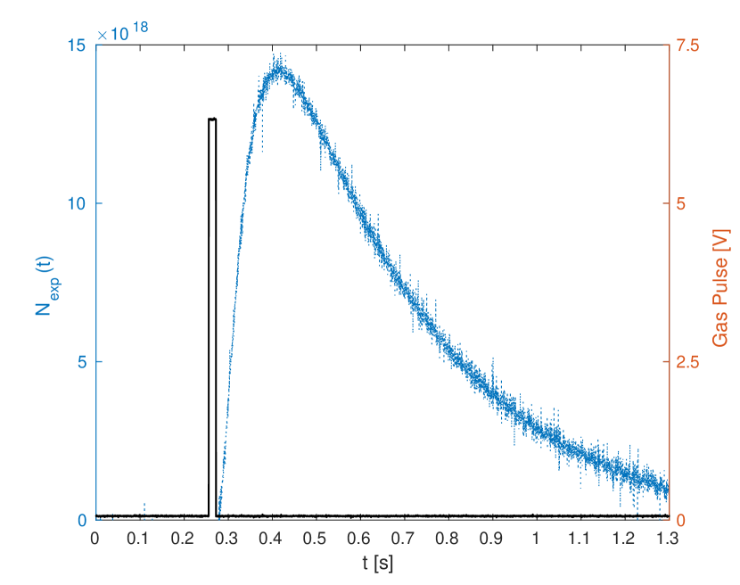
Figure 1: Figure showing time variation of the experimentally measured gas pressure $p_{g}$ (converted into number of particles $N$) on y1-axis, with the applied gas pulse voltage on y2-axis for shot t1111 on ADITYA tokamak. Here, the pulse duration is 16 ms and is switched on in a step function mode at $t\approx 0.256$ s. The BA-IG starts to register the pressure after a gap of $\sim 23$ ms at $t\approx 0.28$ s.

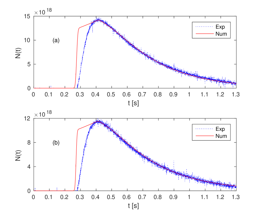
Figure 2: Subplots (a) and (b) represent different piezoelectric valve opening duration of 16 ms and 13 ms, respectively. The red/solid line represents the numerical solution of Eq. (3) obtained by using the DDE23 solver of MATLAB, MATLAB (2015) and it is clear that the simple linear DDE model is able to reproduce the main features of the respective experimental data shown by blue/dotted line. The parameters used for generating the numerical solution are $\tau=142.5$ ms, $\alpha=2.72$, $a=1.0$, $Q_{0}=7.728\times 10^{20}$, while $\delta=9.027$ ms, $t_{0}=275$ ms for subplot (a), and $\delta=7.334$ ms, $t_{0}=272$ ms for subplot (b), respectively.

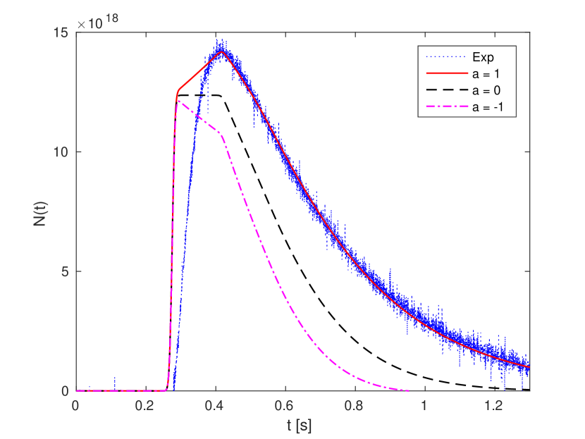
Figure 3: To simulate the effect of wall loading/outgassing in Eq. (3), change of parameter $a$ while keeping all else as in Fig. 2. Here, $a=1$ (red/solid line) and $a=-1$ (magenta/dash-dot) correspond to the wall being a net source and sink of the pre-fill gas, respectively. In case of $a=0$ (black/dash line), the wall plays no role.

In Fig. (1) the y1-axis shows the typical time variation of the total number of gas molecules registered by the BA-IG after they had been administered few tens of ms before by the piezoelectric valve whose voltage pulse is shown on the y2-axis for the same abscissa. For this plot the valve remained open for $16$ ms. The two subplots in Fig. (2) show the comparision of the experimental results (blue/dotted line) with the numerical solution (red/solid line) of Eq. (3) obtained by using the DDE23 solver of MATLAB.MATLAB (2015) Figs. 2(a) and 2(b) correspond to the valve opening time of 16 ms and 13 ms, respectively. It is evident that our simple first-order linear DDE model with external forcing is able to capture the main features of both the experimental profiles. The role of vessel wall acting as a source or sink of hydrogen gas, decided by the sign of parameter $a$ in Eq. (3), is shown in Fig. (3). For typical experimental parameters, it is deduced from a close match of model solution with $a>0$ (red/solid line) and the experimental data (blue/dotted line), for these experiments in particular, that there is a net outgassing.

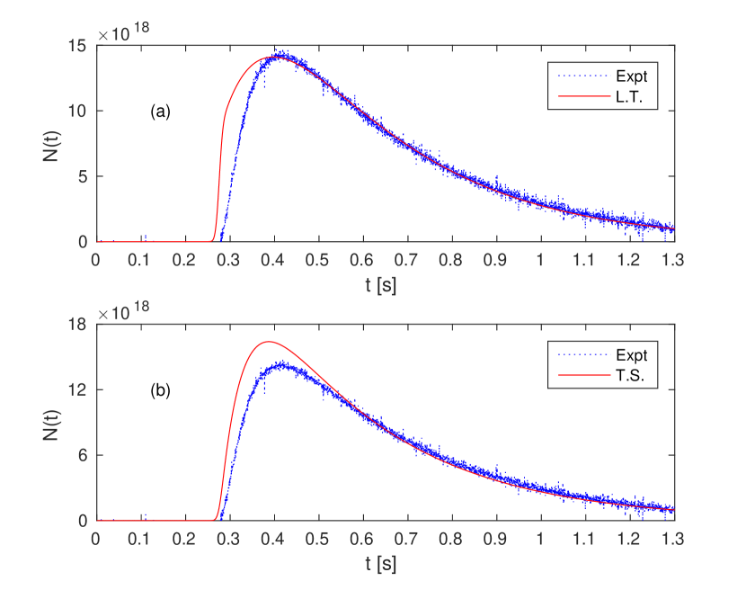
Figure 4: Comparision of the analytical solutions (red/solid line) with experimental result (blue/dotted line), keeping all the parameters same as in Fig. 2(a). Subplot (a) shows the solution obtained using the Laplace transform (L.T.) method (Eq. 8), and subplot (b) shows the solution (Eq. 14) obtained on solving the Taylor series (T.S.) expansion by singular perturbation technique for an IVP type problem.

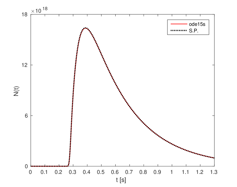
Figure 5: Comparision of singular perturbation derived solution given by Eq. (14) (dot/black) line with that obtained from Eq. (10) using MATLAB’s ode15s solver (solid/red line). An exact match between the two solutions establishes the veracity of the analytical technique.

In Figs. 4(a) and 4(b), we have plotted the comparisions of an experimental data ($\Delta t_{v}=16$ ms) with the solutions obtained by the analytical techniques of Laplace transform and singular perturbation described in sections III.1 and III.2, respectively. It is amply clear that while the Laplace transform solution much closely approximates the experimental data, lending further credence to our model, the singular perturbation solution deviates much more. This is because of the conversion of a DDE into an ODE by using a low-order Taylor series expansion to approximate the time-delay term. It shows that such an approximation is prone to errors. However, to check the veracity of the singular perturbation solution obtained, we have also solved Eq. (10) using the ode15s solver of MATLAB, MATLAB (2015) and the resultant (complete) match with Eq. (14) shown in Fig. (5) validates this analytical technique for application to IVP type singular ODEs.

To finally establish the importance of the delayed negative feedback term in Eq. (3) and main argument of this paper, we have solved it in the limit of a nonexistent delay term ($\tau\approx 0$) with all other parameters being the same as in Fig. 2(a). The results (numerical and analytical) are shown in Fig. (6) and it is immediately clear that there is hardly any match between the model solutions and the experimental result. This major discrepancy shows the necessity of including time-delay in a lumped parameter model of the type given by Eq. (1). Interestingly, it is also seen that all the three solutions viz., numerical, Laplace transform, and singular perturbation converge exactly with each other. Apart from the robustness of the Laplace transform method, this additionally implies that a Taylor series expansion of the delay term is suitable to use only if the delay is sufficiently small.

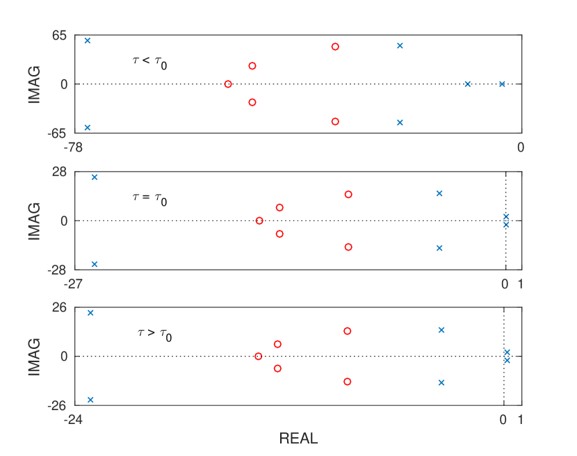
Figure 7: Pole-zero plots for three different time-delay values $\tau=142.5$ ms, $\tau=\tau_{0}\simeq 472$ ms, and $\tau=530$ ms, respectively, in the complex $s$-plane. The pole locations are marked with a cross ($\times$) and the zero locations by a circle ($\circ$).

To better understand the Hopf bifurcation described in section III.3, we first plot the so-called ‘pole-zero’ plots, whose axes represent the real and imaginary part of the complex variable $s$. It will provide the location of the poles and zeros of the transfer function $H(s)$, which will then define the system response depending on whether the poles are real, imaginary, or complex, occur as single or a conjugate pair, and lie in the left-half or right-half of the $s$-plane. For the (fixed) parameters $a$ and $\alpha$ used in this paper, the critical value $\tau_{0}$ is $\sim 472$ ms. It can be seen from Fig. 7(a) that for values of $\tau(<\tau_{0})$, all the poles lie on the left side of the imaginary axis signifying the asymptotic stability of the solutions, while for $\tau=\tau_{0}$ Fig. 7(b) shows, as predicted by the Hopf bifurcation theorem,J.K. Hale (1977) a pair of purely imaginary roots, whereas Fig. 7(c) additionally confirms the presence of Hopf bifurcation, as a complex-conjugate pair of eigenvalues cross, at nonzero speed, from left to the right half-plane i.e., acquire positive real parts, while the remainder of the spectrum stays on the left-hand side of the complex $s$-plane.

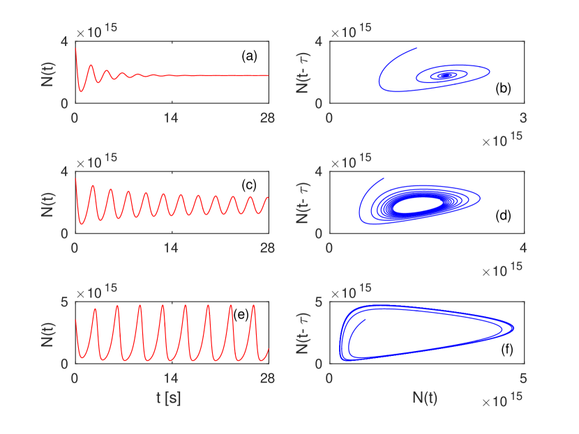
Figure 8: Time variation of number density $N(t)$ and phase portraits for three different time-delays close to the critical value $\tau_{0}$; $\tau=0.41$ for subplots (a) and (b), $\tau=\tau_{0}\simeq 0.472$ for subplots (c) and (d), and $\tau=0.534$ for subplots (e) and (f), respectively, while keeping all other parameters same and as in Figure 2. A supercritical Hopf bifurcation with stable periodic orbits is shown to occur for $\tau>\tau_{0}$.

We now numerically examine the stability of solutions in the neighbourhood of a Hopf bifurcation characterized by the parameter $\tau_{0}$ in absence of external forcing as given by the nonlinear Eq. (6). The presence of a non T-periodic forcing as represented by the Gaussian will not have an impact on the solutions as the problem will remain invariant to arbitrary translations of the origin of time. For $\tau<\tau_{0}$, Fig. 8(a) shows an exponentially damped oscillatory behaviour leading to steady-state values, with the orbits spiraling in to a limit point as seen from the phase portrait in Fig. 8(b). For $\tau=\tau_{0}$, the phase portrait in Fig. 8(d) shows that the limit point bifurcates into a periodic orbit (limit cycle), and Fig. 8(c) displays that the equilibrium state loses stability and results in small amplitude oscillations about the steady state. Lastly, for $\tau>\tau_{0}$, Fig. 8(f) shows that the stable spiral for $\tau=\tau_{0}$ changes into an unstable spiral surrounded by a small, nearly elliptical limit cycle which becomes distorted as $\tau$ moves away from the bifurcation point.S.H. Strogatz (1994) Fig. 8(e) finally establishes the supercritical Hopf bifurcation with stable periodic orbits. In addition, evaluating the analytical condition for our parameters ($a=1,\alpha=2.72$) yields that $\tau_{2}{\rm{Re}}(s^{\prime}(\tau_{0}))\sim 0.18$, which is $>0$. This establishes the bifurcation to be supercritical, thus confirming the numerical solution as well.

V Discussion and Conclusions

In summary, the new and salient features of our model are that it combines the two key mechanisms of delayed negative feedback and external forcing to yield a lumped parameter model in the form of a linear DDE, which is found to reproduce much more accurately the main features of the tokamak pre-fill pressure measurements than a reduced model in the form of a delay free system. This simple, extremely fast, and reasonably accurate model can thus help validate not only the experimental findings of the time variation of the pre-fill pressure, but also that of the main parameters related to the vacuum system such as valve throughput, overall conductance of the pipe network, experimental calibration parameters, requisite pumping speeds, outgassing or pumping by the wall, etc. For example, a detailed calculation of all the distributed pumping and conductances of ADITYA tokamak, incorporating exit/entrance and beaming corrections for molecular gas flow, will be compared with those used in this simple DDE model and published later. Note that in tokamak type fusion devices, accurate measurement of pressure has been found to be necessary for better estimation of particle balance and ion temperature, optimization of discharge cleaning, design and testing of vacuum systems, accountability of tritium, etc.H.F. Dylla (1982)

The model DDE has been solved numerically using a standard solver from MATLAB, MATLAB (2015) and analytically using two different techniques. It is found that a singular perturbation technique can be used to solve a second-order IVP type ODE that results from approximating the delay term by a low-order Taylor series expansion. However, it is also found that such approximations work well only if the delay is small. The Laplace transform method on the other hand, is highly robust and is able to reproduce the main features of the experimental result, but the use of residue theorem during inversion requires the solution of an exponential polynomial type characteristic equation which can have infinite roots. We have therefore used the diagonal Padé approximants to solve for the most dominant poles, and the results are quite satisfactory when compared with the numerical solution.

Since the DDEs are infinite dimensional, they readily admit the problem of bifurcation of steady flow into time-periodic flow, as it is not possible for a time-periodic solution to bifurcate from a steady one in one dimension. Iooss and D.D. Joseph (1980) A Hopf bifurcation is shown to occur at a critical value of time-delay for which the characteristic equation has exactly one pair of conjugate roots on the imaginary axis, and a supercritical bifurcation, where the limit cycle is stable above the bifurcation point is found, numerically as well as by the Poincaré-Lindstedt method. Thus the time-delay needs to be minimized so as to avoid periodic oscillations in $p_{g}$ which occur if $\tau\gtrsim\tau_{0}$, or else, better wall conditioning can control outgassing and lower the value of $a$, which for the same effective pumping speed $\alpha$ increases the critical value $\tau_{0}$.

Although our simple model is unexpectedly accurate in simulating the pre-fill pressure profile, further improvement of the model are necessary to help understand the mismatch between our model solutions and the experimental data, especially during the initial rise of pressure. A possible step in that direction could be the use of neutral type functional differential equation which often arise in the study of two or more simple oscillatory systems with some interconnections between them,J.K. Hale (1977) instead of the retarded type used here.

Figure 6: Effect of nonexistent time-delay ($\tau=10^{-9}$), with all other parameters being same as in Fig. 2(a). Comparision of solutions derived using Matlab’s DDE23 (red/solid) line, singular perturbation (dash-dot/black) line, and Laplace transform with Padé approximants (green/dash) line is shown. An exact match between the singular perturbation and the other two solutions is obtained only in this limit of small $\tau$, thus limiting the use of Taylor series expansion for simplifying DDEs. More importantly, this plot establishes the crucial role played by a finite time-delay.

References

- J.F. O’Hanlon (2003) J.F. O’Hanlon, A User’s Guide to Vacuum Technology, 3rd ed. (John Wiley & Sons, Inc., New Jersey, 2003).
- B.R.F. Kendall and R.E. Pulfrey (1969) B.R.F. Kendall and R.E. Pulfrey, J. Vac. Sci. Technol. 6, 326 (1969).
- K.M. Welch (1973) K.M. Welch, Vacuum 23, 271 (1973).
- Kanazawa (1988) K. Kanazawa, J. Vac. Sci. Technol. A 6, 3002 (1988).
- Ohta, Yoshimura, and Hirano (1983) S. Ohta, N. Yoshimura, and H. Hirano, J. Vac. Sci. Technol. A 1, 84 (1983).
- S.R. Wilson (1987) S.R. Wilson, J. Vac. Sci. Technol. A 5, 2479 (1987).
- J.A. Theil (1994) J.A. Theil, J. Vac. Sci. Technol. A 13, 442 (1994).
- Poschenrieder, Venus, and the ASDEX-Team (1982) W. Poschenrieder, G. Venus, and the ASDEX-Team, J. Nucl. Mater. 111-112, 29 (1982).
- Beuter et al. (2003) A. Beuter, L. Glass, M.C. Mackey, and M.S. Titcombe, eds., in Nonlinear Dynamics in Physiology and Medicine, Interdisciplinary Applied Mathematics, Vol. 25 (Springer-Verlag New York, 2003).
- Kolmanovskii and Myshkis (1999) V. Kolmanovskii and A. Myshkis, Introduction to the Theory and Applications of Functional Differential Equations (Springer-Science+Business Media, B.V., Dordrecht, 1999).
- K.L. Cooke and Grossman (1982) K.L. Cooke and Z. Grossman, J. Math. Anal. Appl. 86, 592 (1982).
- Gopalsamy (1992) K. Gopalsamy, Stability and Oscillations in Delay Differential Equations of Population Dynamics (Springer Science+Business Media, B.V., Dordrecht, 1992).
- Erneux (2009) T. Erneux, Applied Delay Differential Equations (Springer-Verlag, New York, 2009).
- Wesson (2011) J. Wesson, Tokamaks, 4th ed. (Oxford University Press, Oxford, 2011).
- P.V. Kokotović, R.E. O’Malley, Jr., and Sannuti (1976) P.V. Kokotović, R.E. O’Malley, Jr., and P. Sannuti, Automatica 12, 123 (1976).
- P.V. Kokotović (1984) P.V. Kokotović, SIAM Rev. 26, 501 (1984).
- S.H. Strogatz (1994) S.H. Strogatz, Nonlinear Dynamics and Chaos: With Applications to Physics, Biology, Chemistry, and Engineering (Westview Press, Cambridge, MA, 1994).
- Steckelmacher (1986) W. Steckelmacher, Rep. Prog. Phys. 49, 1083 (1986).
- P.A. Redhead, J.P. Hobson, and E.V. Kornelson (1993) P.A. Redhead, J.P. Hobson, and E.V. Kornelson, The Physical Basis of Ultrahigh Vacuum (American Institute of Physics, New York, 1993).
- R.F. Berg (2014) R.F. Berg, J. Vac. Sci. Technol. A 32, 031604 (2014).
- Roth (1989) A. Roth, Vacuum Technology, 2nd ed. (Elsevier Science Publishers B.V., Amsterdam, 1989).
- J. Mallet-Paret and Sell (1996) J. Mallet-Paret and G. Sell, J. Differ. Equations 125, 441 (1996).
- Driver (1977) R. D. Driver, Ordinary and Delay Differential Equations (Springer-Verlag New York Inc., New York, 1977).
- L.E. El’sgol’ts and S.B. Norkin (1973) L.E. El’sgol’ts and S.B. Norkin, Introduction to the Theory and Application of Differential Equations with Deviating Arguments (Academic Press, New York, 1973).
- Bellman and K.L. Cooke (1963) R. Bellman and K.L. Cooke, Differential-Difference Equations (Academic Press, New York, 1963).
- Gu, V.L. Kharitonov, and Chen (2003) K. Gu, V.L. Kharitonov, and J. Chen, Stability of Time-Delay Systems (Springer Science+Business Media, LLC, New York, 2003).
- J.-P. Richard (2003) J.-P. Richard, Automatica 39, 1667 (2003).
- M.F. Reusch et al. (1988) M.F. Reusch, L. Ratzan, N. Pomphrey, and W. Park, SIAM J. Sci. Stat. Comput. 9, 829 (1988).
- P.M. Mäkilä and J.R. Partington (1999) P.M. Mäkilä and J.R. Partington, Int. J. Control 72, 932 (1999).
- Mazanov and K.P. Tognetti (1974) A. Mazanov and K.P. Tognetti, J. Theor. Biol. 46, 271 (1974).
- Bender and Orszag (1999) C. M. Bender and S. A. Orszag, Advanced Mathematical Methods for Scientists and Engineers I (Springer-Verlag New York Inc., New York, 1999).
- A.H. Nayfeh (2004) A.H. Nayfeh, Perturbation Methods (Wiley-VCH Verlag GmbH & Co. KGaA, Weinheim, Germany, 2004).
- Casal and Freedman (1980) A. Casal and M. Freedman, IEEE Trans. Autom. Control 25, 967 (1980).
- Carr (1982) J. Carr, Applications of Centre Manifold Theory (Springer-Verlag New York Inc., New York, 1982).
- MATLAB (2015) MATLAB, Version 8.6 (R2015b) (The MathWorks Inc., Natick, Massachusetts, 2015).
- J.K. Hale (1977) J.K. Hale, Theory of Functional Differential Equations (Springer-Verlag, New York, 1977).
- H.F. Dylla (1982) H.F. Dylla, J. Vac. Sci. Technol. 20, 119 (1982).
- Iooss and D.D. Joseph (1980) G. Iooss and D.D. Joseph, Elementary Stability and Bifurcation Theory (Springer-Verlag, New York, 1980).
- N. van de Wouw, Michiels, and Besselink (2015) N. van de Wouw, W. Michiels, and B. Besselink, Automatica 55, 132 (2015).