On a flow of substance in a channel of network that contains a main arm and two branches

Abstract

We study the motion of a substance in a channel that is part of a network. The channel has 3 arms and consists of nodes of the network and edges that connect the nodes and form ways for motion of the substance. Stationary regime of the flow of the substance in the channel is discussed and statistical distributions for the amount of substance in the nodes of the channel are obtained. These distributions for each of the three arms of the channel contain as particular case famous long-tail distributions such as Waring distribution, Yule-Simon distribution and Zipf distribution. The obtained results are discussed from the point of view of technological applications of the model (e.g., the motion of the substance is considered to happen in a complex technological system and the obtained analytical relationships for the distribution of the substance in the nodes of the channel represents the distribution of the substance in the corresponding cells of the technological chains). A possible application of the obtained results for description of human migration in migration channels is discussed too.

1 Introduction

The studies on the dynamics of complex systems are very intensive in the last decade especially in the area of nonlinear dynamics [3], [4], [11]-[17], [19],[24], [35],[37],[42] - [47] and in the areas of social dynamics and population dynamics [1], [2], [5],[31],[33],[34],[48] - [56]. Networks and the flows in networks are important part of the structure and processes of many complex systems [18, 21, 30]. Research on network flows has roots in the studies on transportation problems [21] and in the studies on migration flows [20, 25, 57]. Today one uses the methodology from the theory of network flows [9] to solve problems connected to e.g., minimal cost of the flow, just in time scheduling or electronic route guidance in urban traffic networks [22].

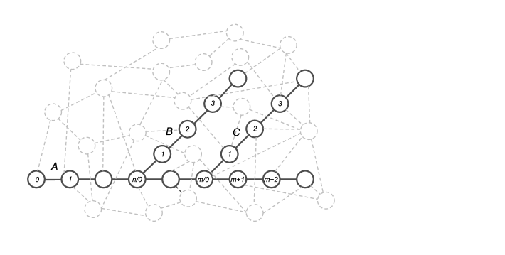
Figure 1: Part of a network and a channel consisting of three arms - $A,B$ and $C$. The nodes of the channel are represented by circles and the edges that connect the nodes are represented by solid lines. The main arm ($A$) splits into two arms at two of the nodes. These nodes are labeled $n/0$ and $m/0$ respectively ($m>n$). The entry nodes of the channels $A,B$ and $C$ are labeled by $0$. The nodes of the network that are not a part of the studied channel are connected by edges that are represented by dashed lines. The assumption below is that the lengths of the arms of the channel are infinite.

A specific feature of the study below is that we consider a channel of a network and this channel consists of three arms. Several types of channels are possible depending on the mutual arrangement of the arms. In this study we shall consider the situation where the channel consists a main arm ($A$, Fig. 1) and two other arms connected to the main one in two different nodes ($n/0$ and $m/0,\ m>n$). In this way the channel has a single arm up to the node $n/0$ where the channel splits to two arms ($A$ and $B$). The first arm $A$ continues up to the node $m/0$ where it also splits to two arms - $A$ and $C$. Thus the studied channel has three arms: $A$, $B$, and $C$.

There are three special nodes in this channel. The first node of the channel arm $A$ (called also the entry node and labeled by the number $0$) is the only node of the channel where the substance may enter the channel from the outside world. After that the substance flows along the channel $A$ up to the node labeled by $n/0$. This is the second special node where the channel splits for the first time and this node (node $n/0$) is the entry node for the second arm $B$ of the channel. The third special node of the network is the node where the channel splits in two arms for the second time (node $m/0$). This node is the entry node for the third arm $C$ of the channel. We assume that the substance moves only in one direction along the channel (from nodes labeled by smaller numbers to nodes labeled by larger numbers). In addition we assume that the substance may quit the channel and may move to the environment. This process will be denoted below as ”leakage”. As the substance can enter the network only through the entry node of the channel arm $A$ then the ”leakage” is possible only in the direction from the channel to the network (and not in the opposite direction).

2 Mathematical formulation of the problem

As we have mentioned above the studied channel consists of three arms. The nodes on each arm are connected by edges and each node is connected only to the two neighboring nodes of the arm exclusive for the first node of the channel arm $A$ that is connected only to the neighboring node and the two other special nodes that are connected to three nodes each. We consider each node as a cell (box), i.e., we consider an array of infinite number of cells indexed in succession by non-negative integers. We assume that an amount $x^{q}$ of some substance is distributed among the cells of the arm $q$ ($q$ can be $A$, $B$ or $C$) and this substance can move from one cell to the neighboring cell.

Let $x_{i}^{q}$ be the amount of the substance in the $i$-th cell on the $q$-th arm. We shall consider channel containing infinite number of nodes in each of its three arms. Then the substance in the $q$-th arm of the channel is

$$x^{q}=\sum\limits_{i=0}^{\infty}x_{i}^{q},\ \ q=\{A,B,C\}.$$ (1)

The fractions $y_{i}^{q}=x_{i}^{q}/x^{q}$ can be considered as probability values of distribution of a discrete random variable $\zeta$ in the corresponding arm of the channel

$$y_{i}^{q}=p^{q}(\zeta=i),\ i=0,1,\dots$$ (2)

The content $x_{i}^{q}$ of any cell may change due to the following 4 processes:

1. Some amount $s^{A}$ of the substance $x^{A}$ enters the main arm $A$ from the external environment through the $0$-th cell;

2. Some amount $s^{q}$ of the substance $x^{q}$ enters the $q$-th arm from the main one through the $n/0$-th or $m/0$-th cell, respectively ($q\in\{B,C\}$);

3. Rate $f_{i}^{q}$ from $x_{i}^{q}$ is transferred from the $i$-th cell into the $i+1$-th cell of the $q$-th arm;

4. Rate $g_{i}^{q}$ from $x_{i}^{q}$ leaks out the $i$-th cell of the $q$-th arm into the environment;

We assume that the process of the motion of the substance is continuous in the time. Then the process can be modeled mathematically by the system of ordinary differential equations:

$$\frac{dx_{0}^{q}}{dt} = s^{q}-f_{0}^{q}-g_{0}^{q};$$

$$\frac{dx_{i}^{q}}{dt} = f_{i-1}^{q}-f_{i}^{q}-g_{i}^{q},\ i=1,2,\dots,;q=\{A,B,C\}$$ (3)

There are two regimes of functioning of the channel: stationary regime and non-stationary regime. What we shall discuss below is the stationary regime of functioning of the channel. In the stationary regime of the functioning of the channel $dx_{i}^{q}/dt=0$, $i=0,1,\dots$. Let us mark the quantities for the stationary case with ^∗. Then from Eqs.(2) one obtains

$$f_{0}^{*q}=s^{*q}-g_{0}^{*q};\ \ f_{i}^{*q}=f_{i-1}^{*q}-g_{i}^{*q}.$$ (4)

This result can be written also as

$$f_{i}^{*q}=s^{*q}-\sum\limits_{j=0}^{i}g_{j}^{*q}$$ (5)

Hence for the stationary case the situation in the each arm is determined by the quantities $s^{*q}$ and $g_{j}^{*q}$, $j=0,1,\dots$. In this chapter we shall assume the following forms of rules for the motion of substance in Eqs.(2) ($\alpha_{i},\beta_{i},\gamma_{i},\sigma$ are constants)

$$s^{A} = \sigma x_{0}^{A}>0$$

$$s^{B} = \delta_{n}^{A}x_{n}^{A};\ \ s^{C}=\delta_{m}^{A}x_{m}^{A};\ \ 1\geq\delta^{A}_{m,n}\geq 0$$

$$f_{i}^{q} = (\alpha_{i}^{q}+\beta_{i}^{q}i)x_{i}^{q};\ \ \ 1>\alpha_{i}^{q}>0,\ 1\geq\beta_{i}^{q}\geq 0$$

$$g_{i}^{q} = \gamma^{*q}_{i}x_{i}^{q};\ \ \ 1\geq\gamma_{i}^{*q}\geq 0\to\textrm{non-uniform leakage in the nodes}$$ (6)

$\gamma^{*}_{i}$ is a quantity specific for the present study. ${\gamma_{i}^{*}}^{A}=\gamma_{i}^{A}+\delta_{i}$ describes the situation with the leakages in the cells on the main arm $A$. We shall assume that $\delta_{i}^{B}=0$, $\delta_{i}^{C}=0$ for all $i$ and $\delta_{i}^{A}=0$ for all $i$ except for $i=n$ and $i=m$. This means that in the $n$-th node in addition to the usual leakage $\gamma_{n}^{A}$ there is additional leakage of substance given by the term $\delta_{n}^{A}x_{n}^{A}$ and this additional leakage supplies the substance that then begins its motion along the second arm of the channel. Furthermore in the $m$-th node (where the main arm of the channel splits for the second time) in addition to the usual leakage $\gamma_{m}^{A}$ there is additional leakage of substance given by the term $\delta_{m}^{A}x_{m}^{A}$ and this additional leakage supplies the substance that then begins its motion along the third arm of the channel.

On the basis of all above the model system of differential equations for each arm of the channel becomes

$$\frac{dx_{0}^{q}}{dt} = s^{q}-\alpha_{0}^{q}x_{0}^{q}-\gamma_{0}^{*q}x_{0}^{q};$$

$$\frac{dx_{i}^{q}}{dt} = [\alpha_{i-1}^{q}+(i-1)\beta_{i-1}^{q}]x_{i-1}^{q}-(\alpha_{i}^{q}+i\beta_{i}^{q}+\gamma_{i}^{*q})x_{i}^{q};\ \ i=1,2,\dots$$ (7)

Below we shall discuss the situation in which the stationary state is established in the entire channel. Then $dx_{0}^{q}/dt=0$ from the first of the Eqs.(2). Hence

$$x_{0}^{q}=\frac{s^{q}}{\alpha_{0}^{q}+{\gamma_{0}^{*}}^{q}}\ \ .$$ (8)

For the main arm $A$ it follows that $\sigma=\alpha_{0}^{A}+\gamma_{0}^{A}$. This means that $x_{0}^{A}$ (the amount of the substance in the $0$-th cell of the arm $A$) is free parameter. For the arm $B$ and $C$, $dx_{0}^{k}/dt=0$ follows that

$$x_{0}^{*B}=\frac{\delta_{n}^{A}x_{n}^{*A}}{\alpha_{0}^{B}+\gamma_{0}^{B}};\ \ x_{0}^{*C}=\frac{\delta_{m}^{A}x_{m}^{*A}}{\alpha_{0}^{C}+\gamma_{0}^{C}}.$$ (9)

The solution of Eqs.(2) is (see Appendix A)

$$x_{i}^{A}=x_{i}^{*A} + \sum\limits_{j=0}^{i}b_{ij}^{A}\exp[-(\alpha_{j}^{A}+j\beta_{j}^{A}+\gamma_{j}^{*A})t];\ \ i=1,2,\dots$$

$$x_{i}^{q}=x^{*q}_{i} + \sum_{j=0}^{i}b^{q}_{ij}\exp[-(\alpha_{j}^{q}+j\beta_{j}^{q}+\gamma_{j}^{*q})t],i=1,2,\dots;q=\{B,C\}$$

where $x_{i}^{*q}$ is the stationary part of the solution. For $x_{i}^{*q}$ one obtains the relationship (just set $dx^{q}/dt=0$ in the second of Eqs.(2))

$$x_{i}^{*q}=\frac{\alpha_{i-1}^{q}+(i-1)\beta_{i-1}^{q}}{\alpha_{i}^{q}+i\beta_{i}^{q}+\gamma_{i}^{*q}}x_{i-1}^{*q},\ i=1,2,\dots;q=\{A,B,C\}$$ (11)

The corresponding relationships for the coefficients $b_{ij}^{q}$ are ($i=1,\dots,q=\{A,B,C\}$):

$$b_{ij}^{q}=\frac{\alpha_{i-1}^{q}+(i-1)\beta_{i-1}^{q}}{(\alpha_{i}^{q}-\alpha_{j}^{q})+(i\beta_{i}^{q}-j\beta_{j}^{q})+(\gamma_{i}^{*q}-\gamma_{j}^{*q})}b_{i-1,j}^{q},\ j=0,1,\dots,i-1,$$ (12)

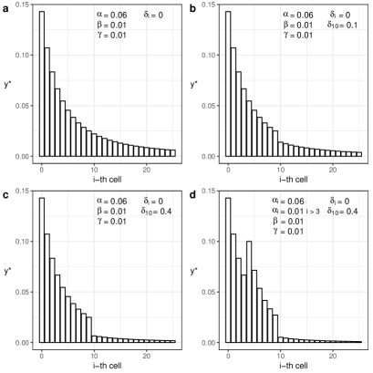
Figure 2: The distribution of the substance in the main arm of the channel described by the Eq.(14) for various values of the parameters $\gamma_{i}^{*}$. Values of the parameters $\alpha_{i}=0.08,\ \beta_{i}=0.01$ and $\gamma_{i}=0.01$ are fixed. The figures show the influence of different choices of the parameter $\gamma_{i}^{*}(\delta_{i})$ on the shape of the distribution. Figure (3a): $\delta_{i}^{A}=0$. There is a flow of substance only in the main arm $A$ of the channel. Figure (3b): $\delta_{i}^{A}=0,\ \delta_{5}^{A}=0.01$. In addition to the main arm, there is a flow of substance in the second arm $B$ of the channel too. Figure (3c): $\delta_{i}^{A}=0,\ \delta_{5}^{A}=0.1,\ \delta_{10}^{A}=0.1$. In this case the substance flows in all three arms of the channel. In addition to the main channel, the second and third channels are also present. Figure (3d): $\delta_{i}=0,\ \delta_{5}=0.1,\ \delta_{10}=0.4$.

From Eq.(11) one obtains

$${x_{i}^{q}}^{*}=\frac{\prod\limits_{j=0}^{i-1}[\alpha_{i-j-1}^{q}+(i-j-1)\beta_{i-j-1}^{q}]}{\prod\limits_{j=0}^{i-1}\alpha_{i-j}^{q}+(i-j)\beta_{i-j}^{q}+{\gamma^{q}}^{*}_{i-j}}{x_{0}^{q}}^{*}$$ (13)

The form of the corresponding stationary distribution ${y_{i}^{q}}^{*}={x_{i}^{q}}^{*}/{x^{q}}^{*}$ (where ${x^{q}}^{*}$ is the amount of the substance in all of the cells of the arm of the channel) is

$${y_{i}^{q}}^{*}=\frac{\prod\limits_{j=0}^{i-1}[\alpha_{i-j-1}^{q}+(i-j-1)\beta_{i-j-1}^{q}]}{\prod\limits_{j=0}^{i-1}[\alpha_{i-j}^{q}+(i-j)\beta_{i-j}^{q}+{\gamma^{q}}^{*}_{i-j}]}{y_{0}^{q}}^{*}$$ (14)

To the best of our knowledge the distribution presented by Eq.(14) was not discussed up to now outside our research group, i.e. this is a new statistical distribution. Let us write the values of this distribution for the first 5 nodes of the main arm of the channel. We assume that the arm $B$ splits at the 3rd node of the arm $A$ and the arm $C$ splits at the 5th node of the arm $A$. Thus the values of the distribution for the first 5 nodes of the channel $A$ are

$$y_{1}^{A^{*}} = y_{0}^{A^{*}}\frac{\alpha_{0}^{A}}{\alpha_{1}^{A}+\beta_{1}^{A}+\gamma_{1}^{A}}$$

$$y_{2}^{A^{*}} = y_{0}^{A^{*}}\frac{\alpha_{0}^{A}}{\alpha_{1}^{A}+\beta_{1}^{A}+\gamma_{1}^{A}}\frac{\alpha_{1}^{A}+\beta_{1}^{A}}{\alpha_{2}^{A}+2\beta_{2}^{A}+\gamma_{2}^{A}}$$

$$y_{3}^{A^{*}} = y_{0}^{A^{*}}\frac{\alpha_{0}^{A}}{\alpha_{1}^{A}+\beta_{1}^{A}+\gamma_{1}^{A}}\frac{\alpha_{1}^{A}+\beta_{1}^{A}}{\alpha_{2}^{A}+2\beta_{2}^{A}+\gamma_{2}^{A}}\frac{\alpha_{2}^{A}+2\beta_{2}^{A}}{\alpha_{3}^{A}+3\beta_{3}^{A}+\gamma_{3}^{A}+\delta_{3}}$$

$$y_{4}^{A^{*}} = y_{0}^{A^{*}}\frac{\alpha_{0}^{A}}{\alpha_{1}^{A}+\beta_{1}^{A}+\gamma_{1}^{A}}\frac{\alpha_{1}^{A}+\beta_{1}^{A}}{\alpha_{2}^{A}+2\beta_{2}^{A}+\gamma_{2}^{A}}\frac{\alpha_{2}^{A}+2\beta_{2}^{A}}{\alpha_{3}^{A}+3\beta_{3}^{A}+\gamma_{3}^{A}+\delta_{3}}\frac{\alpha_{3}^{A}+3\beta_{3}^{A}}{\alpha_{4}^{A}+4\beta_{4}^{A}+\gamma_{4}^{A}}$$

$$y_{5}^{A^{*}} = y_{0}^{A^{*}}\frac{\alpha_{0}^{A}}{\alpha_{1}^{A}+\beta_{1}^{A}+\gamma_{1}^{A}}\frac{\alpha_{1}^{A}+\beta_{1}^{A}}{\alpha_{2}^{A}+2\beta_{2}^{A}+\gamma_{2}^{A}}\frac{\alpha_{2}^{A}+2\beta_{2}^{A}}{\alpha_{3}^{A}+3\beta_{3}^{A}+\gamma_{3}^{A}+\delta_{3}}\frac{\alpha_{3}^{A}+3\beta_{3}^{A}}{\alpha_{4}^{A}+4\beta_{4}^{A}+\gamma_{4}^{A}}\times$$

$$\frac{\alpha_{4}^{A}+4\beta_{3}^{A}}{\alpha_{5}^{A}+5\beta_{4}^{A}+\gamma_{5}^{A}+\delta_{5}}$$

Let us show that the distribution described by Eq.(14) contains as particular cases several famous distributions, e.g., Waring distribution, Zipf distribution, and Yule-Simon distribution. In order to do this we consider the particular case when $\beta_{i}^{q}\neq 0$ and write $x_{i}^{q}$ from Eq.(13) by means of the new notations $k_{i}^{q}=\alpha_{i}^{q}/\beta_{i}^{q}$; $a_{i}^{q}={\gamma^{q}}^{*}_{i}/\beta_{i}^{q}$; $b_{i}^{q}=\beta_{i-1}^{q}/\beta_{i}^{q}$. Let us now consider the particular case where $\alpha_{i}^{q}=\alpha^{q}$ and $\beta_{i}^{q}=\beta^{q}$ for $i=0,1,2,\dots$, $q=\{A,B,C\}$. Then from Eq.(14) one obtains

$${x_{i}^{q}}^{*}=\frac{[k^{q}+(i-1)]!}{(k^{q}-1)!\prod\limits_{j=1}^{i}(k^{q}+j+a_{j})}{x_{0}^{q}}^{*}$$ (16)

where $k^{q}=\alpha^{q}/\beta^{q}$ and $a_{j}^{q}={\gamma^{q}}^{*}_{j}/\beta^{q}$. Let us now consider the particular case where $a_{0}^{q}=\dots=a_{N}^{q}$. In this case the distribution for $P^{q}(\zeta=i)$ for ${y_{i}^{q}}^{*}={x_{i}^{q}}^{*}/{x^{q}}^{*}$ is:

$$P^{q}(\zeta=i) = P^{q}(\zeta=0)\frac{(k^{q}-1)^{[i]}}{(a^{q}+k^{q})^{[i]}};\ \ {k^{q}}^{[i]}=\frac{(k^{q}+i)!}{k^{q}!};\ i=1,2,\dots$$ (17)

$P^{q}(\zeta=0)={y_{0}^{q}}^{*}={x_{0}^{q}}^{*}/{x^{q}}^{*}$ is the percentage of substance that is located in the first cell of the channel. Let this percentage be ${y_{0}^{q}}^{*}=\frac{a^{q}}{a^{q}+k^{q}}$ This case corresponds to the situation where the amount of substance in the first cell is proportional of the amount of substance in the entire channel. In this case Eq.(17) is reduced to:

$$P^{q}(\zeta=i) = \frac{a^{q}}{a^{q}+k^{q}}\frac{(k^{q}-1)^{[i]}}{(a^{q}+k^{q})^{[i]}};\ \ {k^{q}}^{[i]}=\frac{(k^{q}+i)!}{k^{q}!};\ i=1,2,\dots;q=\{A,B,C\}$$

For all $q$ the distribution (2) is exactly the Waring distribution (probability distribution of non-negative integers named after Edward Waring - the 6th Lucasian professor of Mathematics in Cambridge from the 18th century) [27, 28]. Waring distribution has the form

$$p_{l}=\rho\frac{\alpha_{(l)}}{(\rho+\alpha)_{(l+1)}};\ \alpha_{(l)}=\alpha(\alpha+1)\dots(\alpha+l-1)$$ (19)

$\rho$ is called the tail parameter as it controls the tail of the Waring distribution. Waring distribution contains various distributions as particular cases. Let $l\to\infty$ Then the Waring distribution is reduced to the frequency form of the Zipf distribution [10] $p_{l}\approx\frac{1}{l^{(1+\rho)}}$. If $\alpha\to 0$ the Waring distribution is reduced to the Yule-Simon distribution [40] $p(\zeta=l\mid\zeta>0)=\rho B(\rho+1,l)$, where $B$ is the beta-function.

3 Discussion

On the basis of the obtained analytical relationships for the distribution of the substance in three arms of the channel we can make numerous conclusions. Let us consider the distribution in the main channel $A$ described by Eq. (14) from the last section (we have to set $q=A$). Below we shall omit the index $A$ keeping in the mind that we are discussing the main arm of the channel. Let us denote as $y_{i}^{*(1)}$ the distribution of the substance in the cells of the main arm of the channel for the case of lack of second and third arms. Let $y_{i}^{*(2)}$ be the distribution of the substance in the cells of the main arm of the channel in the case of the presence of second and the absence of the third arm of the channel. Finally, let $y_{i}^{*(3)}$ be the distribution of the substance in the cells of the main arm of the channel in the case of the presence of both the second and third arms. From the theory in the previous section one easily obtains the relationship

$$\frac{y_{i}^{*(1)}}{y_{i}^{*(r)}}=\prod\limits_{j=0}^{i-1}\frac{\alpha_{i-j}+(i-j)\beta_{i-j}+\gamma^{*}_{i-j}}{\alpha_{i-j}+(i-j)\beta_{i-j}+\gamma_{i-j}}=\prod\limits_{j=0}^{i-1}\left[1+\frac{\delta_{i-j}}{\alpha_{i-j}+(i-j)\beta_{i-j}+\gamma_{i-j}}\right],$$

where $r$ can be $2$ or $3$. If there are no second and third arms of the channel then the distribution of the substance in the arm $A$ has a standard form of a long-tail distribution like the distribution shown in Fig. 2a. In the case of presence of additional arms $B$ and $C$ and if $i<n$ then $\delta_{i}=0$ and there is no difference between the distribution of the substances in the channel with single arm and in the channel with two arms. The difference arises at the splitting cell $n/0$. As it can be easily calculated for $i\geq n$ and $i<m$ Eq.(3) reduces to

$$\frac{y_{i}^{*(2)}}{y_{i}^{*(1)}}=\frac{1}{1+\frac{\delta_{n}}{\alpha_{n}+n\beta_{n}+\gamma_{n}}},\ \ m>i\geq n$$ (21)

Eq.(21) shows clearly that the presence of the second arm of the channel changes the distribution of the substance in the main arm of the channel. The ”leakage” of the substance to second arm of the channel may reduce much the tail of the distribution of substance in the main arm of the channel. This can appear as a kink in the distribution similar to the kink that can be seen at Fig. 2b.

When $i\geq m$ Eq.(3) reduces to

$$\frac{y_{i}^{*(3)}}{y_{i}^{*(1)}}=\left[\frac{1}{1+\frac{\delta_{n}}{\alpha_{n}+n\beta_{n}+\gamma_{n}}}\right]\left[\frac{1}{1+\frac{\delta_{m}}{\alpha_{m}+m\beta_{m}+\gamma_{m}}}\right],\ \ i\geq m$$ (22)

Eq.(22) shows that the ”leakage” of the substance through both the second and the third arms may reduce even more the tail of the distribution of substance in the main arm than only through the second arm. This reduction becomes extremely strong for large values of $\delta_{n}$ and $\delta_{m}$ (Figs. 2c and 2d). Furthermore, it is easily seen that the presence of the third arm of the channel does not change the distribution of the substance in the second arm. We note that the form of the distribution (14) can be different for different values of the parameters of the distribution. One interesting form of the distribution can be observed in Fig. 2d and this form is different than the conventional form of a long-tail discrete distribution shown in Fig. 2a. Thus at Fig. 2 one can obtain visually a further impression that the distribution (14) is more general than the Waring distribution.

4 Concluding remarks

In this text we have discussed one possible case of motion of substance through a network. Namely our attention was concentrated on the directed motion of substance in a channel of network. Specific feature of the study is that the channel consists of three arms: main arm and two other arms that split from the main arm. We propose a mathematical model of the motion of the substance through the channel and our interest in this study was concentrated on the stationary regime of the motion of the substance through the arms of the channel. The main outcome of the study is the obtained distributions of substance along the cells of the channel. These distributions have a very long tail in the form of the distributions depends on the numerous parameters that regulate the motion of the substance through the channel. Nevertheless we have shown that all of the distributions (i.e. the distributions of the substance along the three arms of the channel) contain as particular case the long-tail discrete Waring distribution which is famous because of the fact that it contains as particular cases the Zipf distribution and the Yule-Simon distribution that are much used in the modeling of complex natural, biological, and social systems.

The model discussed above can be used for study of motion of substance through cells of technological systems. The model can be applied also for study of other system such as channels of human migration or flows in logistic channels. Initial version of the model (for the case of channel containing one arm) was applied for modeling dynamics of citations and publications in a group of researchers [38]. Let us make several notes on the application in the case of human migration as the study of human migration is an actual research topic [6] - [8], [26], [29], [32], [36], [39], [41], [57] - [61]. In this case of application of the theory the nodes are the countries that form the migration channel and the edges represents the ways that connect the countries of the channel. Eqs.(21,22) show that the additional arms of the channel can be used to decrease the ”pressure” of migrants in the direction of the more preferred countries that are relatively away from the initial countries of the channel. This may be done by appropriate increase of the coefficients $\delta_{n}$ and $\delta_{m}$ in Eqs.(21,22).

The research presented above is connected to the actual topic of motion of different types of substances along the nodes and the edges of various kinds of networks. We intend to continue this research by study of more complicated kinds of channels and by use more sophisticated model that accounts for more kinds of processes that may happen in connection with the studied network flows.

A Proof that Eq.(2) is a solution of Eqs.(2) for main arm of the channel

Let us consider the first equation from Eqs.(2) for main arm. In this case $i=0$ and Eqs.(2) becomes $x_{0}^{A}=x_{0}^{*A}+b_{00}^{A}\exp[-(\alpha_{0}^{A}+~{}\gamma_{0}^{A})t]$. The substitution of the last relationship in the first of the Eqs.(2) leads to the relationship

$$0=(\sigma_{0}-\alpha_{0}^{A}-\gamma_{0}^{*A})x_{0}^{*}+b_{00}^{A}\sigma_{0}\exp[-(\alpha_{0}^{A}+\gamma_{0}^{*A})t].$$ (23)

Let us assume $\sigma_{0}=\alpha_{0}^{A}+\gamma_{0}^{*A}$ and $b_{00}^{A}=0$. Then Eqs.(2) describes the solution of the first of Eqs.(2).

Let us now consider Eqs.(2) for the main arm of the channel for $i=1,2,\dots$ Let us fix $i$ and substitute the first of Eqs.(2) in the corresponding equation from Eqs.(2). The result is

$$\sum\limits_{j=0}^{i-1}\exp[-(\alpha_{j}^{A}+j\beta_{j}^{A}+\gamma_{j}^{*A})t]\big{\{}-b_{ij}^{A}(\alpha_{j}^{A}+j\beta_{j}^{A}+\gamma_{j}^{*A})-$$ (24)

$$-b_{i-1,j}^{A}[\alpha_{i-1}^{A}+(i-1)\beta_{i-1}^{A}]+b_{ij}^{A}(\alpha_{i}^{A}+i\beta_{i}^{A}+\gamma_{i}^{*A})\big{\}}=0$$

As it can be seen from Eq.(12), Eq.(24) is satisfied.

References

- [1] Albert, R., Barabasi, A.-L. Statistical mechanics of complex networks. Rev. Mod. Phys. 74, 47 – 97 (2002).
- [2] Amaral, L. A. N., Ottino, J. M. Complex networks. Augmenting and framework for the study of complex systems. Eur. Phys. J. B 38, 147 – 162 (2004).
- [3] Ausloos, M., Gadomski, A., Vitanov, N. K. (2014). Primacy and ranking of UEFA soccer teams from biasing organization rules. Physica Scripta, 89, 108002 (2014).
- [4] Ausloos, M., Cloots, R., Gadomski, A., Vitanov, N. K. Ranking structures and rank–rank correlations of countries: The FIFA and UEFA cases. International Journal of Modern Physics C, 25, 1450060 (2014).
- [5] Boccaletti S., Latora V., Moreno Y., Chavez M., Hwang D. U. Complex networks: Structure and dynamics. Physics Reports, 424, 175 – 308 (2006).
- [6] Borjas G. J. Economic theory and international migration. International Migration Review 23, 457 - 485 (1989).
- [7] Bracken I., Bates J. J. Analysis of gross migration profiles in England and Wales: some developments in classification. Environment and Planning A 15, 343-355 (1983).
- [8] Champion A. G., Bramley G., Fotheringham A. S., Macgill J., Rees P. H. A migration modelling system to support government decision-making. In Stillwell J., Geertman S. (Eds.) Planning support systems in practice. p.p. 257 - 278 Springer Verlag, Berlin (2002).
- [9] Chan W.-K. Theory of nets: Flows in networks. Wiley, New York, 1990.
- [10] Chen W.-C.. On the weak form of the Zipf’s law. Journal of Applied Probability 17, 611 - 622 (1980).
- [11] Dimitrova, Z. On traveling waves in lattices: The case of Riccati lattices. Journal of Theoretical and Applied Mechanics, 42 , 3 - 22 (2012).
- [12] Dimitrova, Z. I., Vitanov, K. N. Integrability of differential equations with fluid mechanics application: from Painleve property to the method of simplest equation. Journal of Theoretical and Applied Mechanics, 43, 31 - 42 (2013).
- [13] Dimitrova, Z. I. Numerical investigation Of nonlinear Waves connected To blood flow in an elastic tube with variable radius. Journal of Theoretical and Applied Mechanics, 45, 79 - 92 (2015).
- [14] Dimitrova, Z. I., Vitanov, N. K. Influence of adaptation on the nonlinear dynamics of a system of competing populations. Physics Letters A, 272, 368 - 380 (2000).
- [15] Dimitrova, Z. I., Vitanov, N. K. Dynamical consequences of adaptation of the growth rates in a system of three competing populations. Journal of Physics A: Mathematical and General, 34, 7459 - 7473 (2001).
- [16] Dimitrova, Z. I., Vitanov, N. K. Adaptation and its impact on the dynamics of a system of three competing populations. Physica A: Statistical Mechanics and its Applications, 300, 91 - 115 (2001).
- [17] Dimitrova, Z. I., Vitanov, N. K. Chaotic pairwise competition. Theoretical Population Biology, 66, 1 - 12 (2004).
- [18] Dorogovtsev, S. N., Mendes, J. F. F. Evolution of networks. Advances in Physics, 51, 1079 – 1187 (2002).
- [19] Nikolova, E. V., Jordanov, I. P., Dimitrova, Z. I., Vitanov, N. K. Nonlinear evolution equation for propagation of waves in an artery with an aneurysm: An exact solution obtained by the modified method of simplest equation. pp. 131 - 144 in K. Georgiev, M. Todorov, I. Georgiev (Eds.) Advanced Computing in Industrial Mathematics. Springer, Cham, 2018.
- [20] Fawcet, J. T.. Networks, linkages, and migration systems. International Migration Review, 23 (1989), 671 - 680 (1989).
- [21] Ford Jr., L. D., Fulkerson, D. R. Flows in Networks. Princeton University Press, Princeton, NJ, 1962.
- [22] Gartner, N. H., Importa G. (Eds.) Urban traffic networks. Dynamic flow modeling and control. Springer, Berlin, 1995.
- [23] Gurak D. T., Caces F.. Migration networks and the shaping of migration systems. In: Kitz M.M., Lim L. L., Zlotnik H. (Eds.) International migration systems: A global approach.p.p. 150-176 Clarendon Press, Oxford, (1992).
- [24] Kantz, H., Holstein, D., Ragwitz, M., Vitanov, N. K. . Markov chain model for turbulent wind speed data. Physica A: Statistical Mechanics and its Applications, 342, 315 - 321 (2004)
- [25] Harris, J. R.,Todaro, M. P. Migration, unemployment and development: A two-sector analysis. The American Economic Review, 60, 126 – 142 (1970).
- [26] Hotelling H. A mathematical theory of migration. Environment and Planning 10, 1223 - 1239 (1978).
- [27] Irwin J. O. The place of mathematics in medical and biological sciences. Journal of the Royal Statistical Society 126, 1 - 44 (1963).
- [28] Irwin J. O. The generalized Waring distribution applied to accident theory. Journal of the Royal Statistical Society 131, 205 - 225 (1968).
- [29] Lee E. S. A theory of migration. Demography 3, 47 - 57 (1966).
- [30] Lu, J., Yu, X., Chen, G., Yu, W. (Eds.) Complex systems and networks. Dynamics, controls and applications. Springer, Berlin (2016).
- [31] Marsan, G. A., Bellomo, N., Tosin, A. Complex systems and society: Modeling and simulation. Springer, New York (2013).
- [32] Massey D. S., Arango J., Hugo G., Kouaougi A., Pellegrino A., Edward Taylor J.. Theories of international migration: A review and appraisal. Population and Development Review 19, 431 - 466 (1993).
- [33] Pastor-Satorras, R., Vespignani, A. Epidemic dynamics and endemic states in complex networks. Physical Review E 63, 066117 (2001).
- [34] Petrov, V., Nikolova, E., Wolkenhauer, O. Reduction of nonlinear dynamic systems with an application to signal transduction pathways. IET Systems Biology, 1, 2 – 9 (2007).
- [35] Panchev, S., Spassova, T., Vitanov, N. K. Analytical and numerical investigation of two families of Lorenz-like dynamical systems. Chaos, Solitons & Fractals, 33, 1658 - 1671 (2007).
- [36] Puu T. Hotelling’s migration model revisited. Environment and Planning 23, 1209 - 1216 (1991).
- [37] Sakai, K., Managi, S., Vitanov, N. K., Demura, K. Transition of chaotic motion to a limit cycle by intervention of economic policy: an empirical analysis in agriculture. Nonlinear dynamics, psychology, and life sciences, 11, 253 - 265 (2007).
- [38] Schubert A., Glänzel W. A dynamic look at a class of skew distributions. A model with scientometric application. Scientometrics 6, 149 – 167 (1984).
- [39] Simon J. H. The economic consequences of migration. The University of Michnigan Press, Ann Arbor, MI, 1999.
- [40] Simon H. A.. On a class of skew distribution functions. Biometrica 42, 425 – 440 (1955).
- [41] Skeldon R. Migration and development: A global perspective. Routledge, London, 1992.
- [42] Vitanov, N. K., Dimitrova, Z. I. Application of the method of simplest equation for obtaining exact traveling-wave solutions for two classes of model PDEs from ecology and population dynamics. Communications in Nonlinear Science and Numerical Simulation, 15, 2836 - 2845 (2010).
- [43] Vitanov, N. K., Dimitrova, Z. I. . On waves and distributions in population dynamics. BIOMATH, 1, 1209253 (2012).
- [44] Vitanov, N. K., Hoffmann, N. P., Wernitz, B. Nonlinear time series analysis of vibration data from a friction brake: SSA, PCA, and MFDFA. Chaos, Solitons & Fractals, 69, 90 - 99 (2014).
- [45] Vitanov, N. K., Dimitrova, Z. I., Vitanov, K. N. (2015). Modified method of simplest equation for obtaining exact analytical solutions of nonlinear partial differential equations: further development of the methodology with applications. Applied Mathematics and Computation, 269, 363 - 378 (2015).
- [46] Vitanov, N. K., Ausloos, M. Test of two hypotheses explaining the size of populations in a system of cities. Journal of Applied Statistics, 42, 2686 - 2693 (2015).
- [47] Vitanov N. K., Dimitrova Z. I.,Ivanova T. I.. On solitary wave solutions of a class of nonlinear partial differential equations based on the function . Applied Mathematics and Computation 315, 372 - 380 (2017).
- [48] Vitanov N. K. Science dynamics and research production: Indicators, indexes, statistical laws and mathematical models. Springer, Cham, 2016.
- [49] Vitanov N. K., Jordanov I. P., Dimitrova Z. I.. On nonlinear dynamics of interacting populations: Coupled kink waves in a system of two populations. Communications in Nonlinear Science and Numerical Simulation 14, 2379 - 2388 (2009)
- [50] Vitanov N. K., Jordanov I. P., Dimitrova Z. I.. On nonlinear population waves. Applied Mathematics and Computation 215, 2950 - 2964 (2009).
- [51] Vitanov N. K., Dimitrova Z. I., Ausloos M. Verhulst-Lotka-Volterra model of ideological struggle. Physica A 389, 4970 - 4980 (2010).
- [52] Vitanov N. K., Ausloos M., Rotundo G. Discrete model of ideological struggle accounting for migration. Advances in Complex Systems 15, Supplement 1, Article number 1250049 (2012).
- [53] Vitanov, N.K., Ausloos, M. Knowledge epidemics and population dynamics models for describing idea diffusion. pp. 69 - 125 in Scharnhorst, A., Börner, K., van den Besselaar, P. (Eds.) Knowledge Epidemics and Population Dynamics Models for Describing Idea Diffusion, berlin, Springer, 2012.
- [54] Vitanov N. K., Dimitrova Z. I., Vitanov K. N. Traveling waves and statistical distributions connected to systems of interacting populations. Computers & Mathematics with Applications 66, 1666 - 1684 (2013).
- [55] Vitanov N.K., Vitanov K. N. Population dynamics in presence of state dependent fluctuations. Computers & Mathematics with Applications 68, 962 - 971. (2013).
- [56] Vitanov, N.K., Ausloos, M. Test of two hypotheses explaining the size of populations in a system of cities. Journal of Applied Statistics, 42, 2686 – 2693 (2015).
- [57] Vitanov N. K., Vitanov K. N. Box model of migration channels. Mathematical Social Sciences 80, 108 - 114 (2016).
- [58] Vitanov, N. K., Vitanov, K.N., Ivanova, T. Box model of migration in channels of migration networks. pp. 203 - 215 in: Georgiev K., Todorov M., Georgiev I. (eds) Advanced Computing in Industrial Mathematics. Studies in Computational Intelligence, vol 728. Springer, Cham ,2018.
- [59] Vitanov, N. K., Vitanov, K.N. On the motion of substance in a channel of network and human migration. Physica A 490 , 1277 - 1290 (2018)
- [60] Weidlich W., Haag G. (Eds.). Interregional migration. Dynamic theory and comparative analysis. Springer, Berlin (1988).
- [61] Willekens F. J. Probability models of migration: Complete and incomplete data. SA Journal of Demography 7, 31 - 43 (1999).