An FFT-based Solution Method for the Poisson Equation on 3D Spherical Polar Grids

Abstract

The solution of the Poisson equation is a ubiquitous problem in computational astrophysics. Most notably, the treatment of self-gravitating flows involves the Poisson equation for the gravitational field. In hydrodynamics codes using spherical polar grids, one often resorts to a truncated spherical harmonics expansion for an approximate solution. Here we present a non-iterative method that is similar in spirit, but uses the full set of eigenfunctions of the discretized Laplacian to obtain an exact solution of the discretized Poisson equation. This allows the solver to handle density distributions for which the truncated multipole expansion fails, such as off-center point masses. In three dimensions, the operation count of the new method is competitive with a naive implementation of the truncated spherical harmonics expansion with $N_{\ell}\approx 15$ multipoles. We also discuss the parallel implementation of the algorithm. The serial code and a template for the parallel solver are made publicly available.

1. Introduction

The numerical solution of the Poisson equation is one of the standard problems in astrophysical fluid dynamics. The Poisson equation is probably encountered most frequently as the equation governing the gravitational field in the Newtonian approximation, but its applications also include constrained formulations of general relativity (e.g. Cordero-Carrión et al., 2009), projection methods for magnetohydrodynamics (Brackbill & Barnes, 1980; LeVeque, 1998), anelastic/low-Mach number flow (Batchelor, 1953; Ogura & Phillips, 1962; Jacobson, 1999), and radiation transport problems (Liebendörfer et al., 2009).

Various methods for the exact or approximate solution of the Poisson equation are commonly used in astrophysical codes. The applicability and usefulness of these methods is typically dictated by the geometry of the physical problem at hand and the discretization technique used for the equations of hydrodynamics. In stellar hydrodynamics approximate spherical symmetry obtains, so that spherical polar grids (including overset grids, Wongwathanarat et al., 2010) are often the method of choice. For such grids, fast algorithms such as the direct use of the three-dimensional Fast Fourier Transform (FFT) (Hockney, 1965; Eastwood & Brownrigg, 1979), multi-grid algorithms (Brandt, 1977), or tree algorithms (Barnes & Hut, 1986) are either not directly applicable, more difficult to implement, or do not offer a good trade-off between computational efficiency and accuracy. One of the most frequently used methods for “star-in-a-box” simulations has long been based on a spherical harmonics expansion of the Green’s function as described by Müller & Steinmetz (1995). Since the gravitational field typically deviates only modestly from spherical symmetry for such problems, the spherical harmonics expansion can be truncated at a low multipole number $N_{\mathrm{\ell}}=10\ldots 20$ for better computational efficiency. The overall operation count of the algorithm is only $\mathcal{O}(N_{r}N_{\theta}N_{\ell})$ for a spherical polar grid with $N_{r}\times N_{\theta}$ zones in the $r$- and $\theta$-direction in the case of axisymmetry (2D), and $\mathcal{O}(N_{r}N_{\theta}N_{\varphi}N_{\ell}^{2})$ in three dimensions (3D) with $N_{\varphi}$ zones in the $\varphi$-direction. The high efficiency of the algorithm has made it the method of choice for several supernova codes employing spherical polar grids such as the the Chimera code (Bruenn et al., 2013), the Aenus code (Obergaulinger et al., 2006), the Fornax code (Burrows et al., 2018), and various offshoots of the Prometheus code (Marek & Janka, 2009; Wongwathanarat et al., 2010). The method has also been adapted (Couch et al., 2013) for simulations of stellar hydrodynamics problems using the Flash code (Fryxell et al., 2000).

Despite its efficiency, this algorithm still has some drawbacks. Above all, it only offers an approximate solution to the Poisson equation. Although the error is usually acceptable when the algorithm is used to obtain the gravitational field, this precludes its use, e.g., for divergence cleaning in the MHD projection method, which requires an exact solution of the discretized Poisson equation. An exact solution is also desirable if one seeks to implement gravitational forces in a momentum-conserving form (Shu, 1992; Livne et al., 2004) and can be exploited to achieve total energy conservation to machine precision (Müller et al., 2010). The truncation of the spherical harmonics expansion is especially problematic when the location of the central density peak of the source does not coincide with the origin of the coordinate system. Although this can be fixed by a judicious choice of the center of the multipole expansion (Couch et al., 2013), such a fix destroys much of the simplicity of the algorithm in spherical polar coordinates. Finally, there are subtle problems with the convergence of the multipole expansion. Couch et al. (2013) noted that a naive implementation of the algorithm can include a spurious self-interaction term that manifestly leads to divergence for large $N_{\ell}$. This can again be fixed – either by the original method of Müller & Steinmetz (1995) or that of Couch et al. (2013) – but more subtle problems still lurk when one projects the source density onto spherical harmonics: Analytically, one has the orthogonality relation

$$\int Y^{*}_{\ell m}Y_{\ell^{\prime}m^{\prime}}\,\mathrm{d}\Omega=\delta_{\ell\ell^{\prime}}\delta_{mm^{\prime}},$$ (1)

which implies that the gravitational field $\Phi$ only contains exactly the same multipole components as the source. This is generally not the case for the discretized integrals. Though the orthogonality relation is easily maintained if either $\ell=0$ or $\ell^{\prime}=0$, and for multipoles of opposite parity, multipoles with $\ell\geq 1$ in the density field will generally give rise to spurious multipoles of arbitrarily high $\ell$. This spurious overlap between spherical harmonics of different $\ell$ and $m$ only vanishes in the limit of infinite spatial resolution. This problem is illustrated further in the Appendix.

In this article, we point out that all of these problems can be avoided by solving the discretized Poisson equation exactly using the discrete analogue of the spherical harmonics expansion in conjunction with the FFT in the $\varphi$-direction. The approach of combining the FFT with Legendre and Chebyshev transforms to exactly invert the Poisson equation is well established in the field of pseudospectral methods (e.g. Fornberg, 1995; Chen et al., 2000; Lai & Wang, 2002; Weatherford et al., 2005). Such pseudospectral approaches can only be combined with finite-volume methods at a cost, however. Since the collocation points of the pseudospectral grid generally differ from the finite-volume grid, mapping is required, which can impact performance and impede parallelization. Moreover, the superior accuracy of pseudospectral methods for the elliptical part of the problem is typically of little advantage when the error is mainly determined by the hyperbolic finite-volume solver; in those cases consistency between the elliptic and hyperbolic solver and the enforcement of physical conservation laws is often a higher priority than the nominal accuracy of the elliptic solver. For these reasons, we here construct an exact algorithm in the flavor of pseudospectral codes that works on the finite-volume grid itself.

The operation count of our algorithm remains competitive with the method of Müller & Steinmetz (1995) in 3D; for an angular resolution of $N_{\theta}\times N_{\varphi}=128\times 256$, the break-even point of the serial algorithm is at $\ell_{\mathrm{max}}\approx 15$. Although the mathematics behind the algorithm is simple and merely based on standard methods from the theory of partial differential equations and linear algebra, it is not currently used in astrophysical fluid dynamics codes and no off-the-shelf implementation is available. Along with the paper, we therefore provide the code of the serial implementation, which uses the Lapack (Anderson et al., 1999) and FFTW (Frigo & Johnson, 2005) libraries, and a template for the parallel version with domain decomposition in $\theta$ and $\varphi$.

Our paper is structured as follows: As a preparation for the solution of the discretized Poisson equation, we recapitulate how the multipole expansion of Müller & Steinmetz (1995) can be obtained directly by separation of variables. We then formulate the discrete analogue of the multipole expansion in Section 3 and also discuss its parallelization. In Section 4 we discuss the efficiency of the serial and parallel version of the algorithm, then proceed to code verification in Section 5, and end with a brief summary in Section 6

2. Multipole Expansion by Separation of Variables

The algorithm of Müller & Steinmetz (1995) for the solution of the Poisson equation for the gravitational potential $\Phi$ and the source density $\rho$,

$$\Delta\Phi=4\pi G\rho,$$ (2)

is usually derived by writing the solution in terms of the Green’s function $\mathcal{G}$, as

$$\Phi(\mathbf{r})=-G\int\mathcal{G}(\mathbf{r}-\mathbf{r^{\prime}})\rho(\mathbf{r^{\prime}})\,\mathrm{d}^{3}\mathbf{r}^{\prime}.$$ (3)

The Green’s function is given by $\mathcal{G}(\mathbf{r}-\mathbf{r^{\prime}})=|\mathbf{r}-\mathbf{r^{\prime}}|^{-1}$, and can be expanded in terms of spherical harmonics $Y_{\ell m}$ as

$$\mathcal{G}(\mathbf{r},\mathbf{r^{\prime}}) = \frac{1}{|\mathbf{r}-\mathbf{r^{\prime}}|}$$

$$= \sum_{\ell=0}^{\infty}\sum_{m=-\ell}^{\ell}\frac{4\pi}{2\ell+1}Y_{\ell m}(\theta,\varphi)Y^{*}_{\ell m}(\theta^{\prime},\varphi^{\prime})\frac{\min(r,r^{\prime})^{\ell}}{\max(r,r^{\prime})^{\ell+1}}.$$

After inserting this expansion into Equation (3) and projecting out the individual multipole components, one can obtain individual multipoles $f_{\ell,m}$ of the solution by integration along the radial direction,

$$f_{\ell,m}(r) = -\frac{4\pi}{2\ell+1}\left[\frac{1}{r^{\ell+1}}\int_{0}^{r}\bar{\rho}_{\ell,m}(r^{\prime})r^{\prime\ell+2}\,\mathrm{d}r^{\prime}\right.$$

$$\left.+r^{\ell}\int_{r}^{\infty}\bar{\rho}_{\ell,m}(r^{\prime})r^{\prime\ell+2}\,\mathrm{d}r^{\prime}\right],$$

and then reconstruct the full solution as

$$\Phi=G\sum_{\ell=0}^{\infty}\sum_{m=-\ell}^{\ell}f_{\ell,m}(r)Y_{\ell m}(\theta,\varphi).$$ (6)

Here $\bar{\rho}_{\ell,m}(r)$ are the multipoles of the source density.

In fact, there is no need to ever invoke the explicit form $\mathcal{G}(\mathbf{r}-\mathbf{r^{\prime}})=|\mathbf{r}-\mathbf{r^{\prime}}|^{-1}$ of the Green’s function and the specific expansion in Equation (2) to derive this solution: Instead, one can directly obtain decoupled ordinary differential equations for $f_{\ell,m}$ by noting that the spherical harmonics are eigenfunctions of the angular part $\Delta_{\Omega}$ of the Laplacian in spherical polar coordinates,

$$\Delta_{\Omega}=\frac{\partial}{\partial\theta}\left(\sin\theta\frac{\partial}{\partial\theta}\right)+\frac{1}{\sin^{2}\theta}\frac{\partial^{2}}{\partial\varphi^{2}}.$$ (7)

Using $\Delta_{\Omega}Y_{\ell m}(\theta,\varphi)=-\ell(\ell+1)Y_{\ell m}(\theta,\varphi)$ after inserting the expansion $\Phi=\sum_{\ell,m}f_{\ell,m}(r)Y_{\ell m}(\theta,\varphi)$ into the Poisson equation then immediately yields decoupled equations for the $f_{\ell,m}$,

$$\frac{1}{r^{2}}\frac{\partial}{\partial r}\left(r^{2}\frac{\partial f_{\ell,m}}{\partial r}\right)-\frac{\ell(\ell+1)}{r^{2}}f_{\ell,m}=4\pi G\int Y_{\ell,m}^{\star}\rho(r,\theta,\varphi)\mathrm{d}\Omega,$$ (8)

which can be solved according to Equation (2). The spherical harmonics themselves are obtained in an analogous manner by first solving the eigenvalue problem for the azimuthal part $\Delta_{\varphi}=\partial^{2}/\partial\varphi^{2}$ of the Laplacian and then solving another set of eigenvalue problems for $\Delta_{\Omega}$.

3. Solution of the Discrete Poisson Equation

For the discretized Poisson equation, one can apply a completely analogous procedure to first obtain the eigenvectors of the $\varphi$-derivative terms in the discrete Laplacian, then the eigenfunctions for $\Delta_{\Omega}$, and finally decoupled equations for the radial dependence of the individual multipole components.

3.1. Discretisation

We discretize the Poisson equation as

$$(\Delta\Phi)_{i,j,k}=(\Delta_{r}\Phi)_{i,j,k}+(\Delta_{\theta}\Phi)_{i,j,k}+(\Delta_{\varphi}\Phi)_{i,j,k}=s_{i,j,k}$$ (9)

where the source is $s_{i,j,k}=4\pi G\rho_{i,j,k}$ and $i$, $j$, and $k$ are the grid indices in the $r$-, $\theta$-, and $\varphi$-direction. Values offset by $1/2$ will be used for quantities at cell interfaces. The discretized operators $\Delta_{r}$, $\Delta_{\theta}$, and $\Delta_{\varphi}$ for the $r$-, $\theta$, and $\varphi$-derivatives are

$$(\Delta_{r}\Phi)_{i,j,k} = \frac{1}{\delta V_{i,j,k}}\left(\frac{\Phi_{i+1,j,k}-\Phi_{i,j,k}}{r_{i+1}-r_{i}}\delta A_{i+1/2,j,k}\right.$$ (10)

$$\left.-\frac{\Phi_{i,j,k}-\Phi_{i-1,j,k}}{r_{i}-r_{i-1}}\delta A_{i-1/2,j,k}\right),$$

$$(\Delta_{\theta}\Phi)_{i,j,k} = \frac{1}{\delta V_{i,j,k}}\left(\frac{\Phi_{i,j+1,k}-\Phi_{i,j,k}}{r_{i}\left(\theta_{j+1}-\theta_{j}\right)}\delta A_{i,j+1/2,k}\right.$$ (11)

$$\left.-\frac{\Phi_{i,j,k}-\Phi_{i,j-1,k}}{r_{i}\left(\theta_{j}-\theta_{j-1}\right)}\delta A_{i,j-1/2,k}\right),$$

$$(\Delta_{\varphi}\Phi)_{i,j,k} = \frac{1}{\delta V_{i,j,k}}\left(\frac{\Phi_{i,j,k+1}-\Phi_{i,j,k}}{r_{i}\sin\theta_{j}\left(\varphi_{k+1}-\varphi_{k}\right)}\delta A_{i,j,k+1/2}\right.$$ (12)

$$\left.-\frac{\Phi_{i,j,k}-\Phi_{i,j,k-1}}{r_{i}\sin\theta_{j}\left(\varphi_{k+1}-\varphi_{k}\right)}\delta A_{i,j,k-1/2}\right).$$

Here, $\delta V$ and $\delta A$ denote cell volumes and interface areas, respectively. We note that this is a second-order accurate (for uniform grids in $r$, $\theta$, and $\varphi$) finite-volume discretisation of the integral form $\oint\nabla\Phi\cdot\mathbf{dA}=4\pi G\int\rho\,\mathrm{d}V$ of the Poisson equation, which allows us to write the energy source term in the Newtonian equations of hydrodynamics such that total energy is conserved to machine precision (Müller et al., 2010).

In order to utilize the FFT in the solution algorithm, we require a uniform grid in $\varphi$ with spacing $\delta\varphi$. For the sake of simplicity, we also use uniform grid spacing in the $\theta$-direction, although this is not required for a solution by separation of variables. In this case, one obtains the following interface surfaces and cell volumes by analytic integration,

$$\delta A_{i+1/2,j,k} = r_{i+1/2}^{2}(\cos\theta_{i,j-1/2,k}-\cos\theta_{i,j+1/2,k})\,\delta\varphi,$$ (13)

$$\delta A_{i,j+1/2,k} = \frac{r_{i+1/2}^{2}-r_{i+1/2}^{2}}{2}\sin\theta_{j+1/2}\,\delta\varphi,$$ (14)

$$\delta A_{i,j,k+1/2} = \frac{r_{i+1/2}^{2}-r_{i+1/2}^{2}}{2}\,\delta\theta,$$ (15)

$$\delta V_{i,j,k} = \frac{r_{i+1/2}^{3}-r_{i-1/2}^{3}}{3}$$

$$\times(\cos\theta_{i,j-1/2,k}-\cos\theta_{i,j+1/2,k})\,\delta\varphi.$$

Before proceeding further, it is convenient to factor out terms that depend on $r$ in $\Delta_{\theta}$ and on $r$ and $\theta$ in $\Delta_{\varphi}$. We therefore define new operators $\hat{\Delta}_{\theta}$ and $\hat{\Delta}_{\varphi}$ such that

$$(\Delta_{\theta}\Phi)_{i,j,k} = \mathcal{R}_{i}\left(\frac{\Phi_{i,j+1,k}-\Phi_{i,j,k}}{\delta\theta}\sin\theta_{j+1/2}\right.$$

$$\left.-\frac{\Phi_{i,j,k}-\Phi_{i,j-1,k}}{\delta\theta}\sin\theta_{j-1/2}\right),$$

$$= \mathcal{R}_{i}(\hat{\Delta}_{\theta}\Phi)_{i,j,k}$$

$$(\Delta_{\varphi}\Phi)_{i,j,k} = \mathcal{R}_{i}\mathcal{S}_{j}\left(\frac{\Phi_{i,j,k+1}-\Phi_{i,j,k}}{\delta\varphi}-\frac{\Phi_{i,j,k}-\Phi_{i,j,k-1}}{\delta\varphi}\right)$$ (18)

$$= \mathcal{R}_{i}\mathcal{S}_{j}(\hat{\Delta}_{\varphi}\Phi)_{i,j,k},$$

where

$$\mathcal{R}_{i} = \frac{3(r_{i+1/2}^{2}-r_{i-1/2}^{2})}{2r_{i}(r_{i+1/2}^{3}-r_{i-1/2}^{3})},$$ (19)

$$\mathcal{S}_{j} = \frac{\delta\theta}{\sin\theta_{j}(\cos\theta_{i,j-1/2,k}-\cos\theta_{i,j+1/2,k})}.$$ (20)

3.2. Description of the Serial Algorithm

To solve the discretized Poisson equation, we first expand the solution in terms of the eigenvectors of $\hat{\Delta}_{\varphi}$ The eigenvectors $h_{m}(k)$ and eigenvalues $\lambda_{\varphi,m}$ are given by

$$h_{m}(k)=e^{2\pi imk/N_{\varphi}},\quad\lambda_{\varphi,m}=\left(\frac{\sin m\,\delta\varphi/2}{\delta\varphi/2}\right)^{2},$$ (21)

where $m$ can take on values between $0$ and $N_{\varphi}-1$. Expressing both $\Phi$ and the source $s$ in terms of the eigenfunctions and Fourier components $g_{i,j,m}$ and $\tilde{s}_{i,j,m}$,

$$\Phi_{i,j,k}=\sum_{m}^{N_{\varphi}-1}g_{i,j,m}h_{m}(k),$$ (22)

$$s_{i,j,k}=\sum_{m=0}^{N_{\varphi}-1}\tilde{s}_{i,j,m}h_{m}(k),$$ (23)

yields

$$\sum_{m=0}^{N_{\varphi}-1}\left[(\Delta_{r}g)_{i,j,m}+\mathcal{R}_{i}(\hat{\Delta}_{\theta}g)_{i,j,m}+\mathcal{R}_{i}\mathcal{S}_{j}\lambda_{\varphi,m}g_{i,j,m}\right]h_{m}(k)$$

$$=\sum_{m=0}^{N_{\varphi}-1}\tilde{s}_{i,j,m}h_{m}(k).$$ (24)

Projecting on the orthogonal eigenvectors yields a partially decoupled system of equations for $g_{i,j,m}$,

$$(\Delta_{r}g)_{i,j,m}+\mathcal{R}_{i}\left[(\hat{\Delta}_{\theta}g)_{i,j,m}+\mathcal{S}_{j}\lambda_{\varphi,m}g_{i,j,m}\right]=\tilde{s}_{i,j,m}.$$ (25)

Here $\tilde{s}_{i,j,m}$ can be obtained efficiently from $s_{i,j,k}$ using the FFT.

To fully decouple the system, we expand $g$ and the $\tilde{s}$ further in terms of the orthonormal eigenvectors of the operator $\hat{\Delta}_{\theta}+\mathcal{S}_{j}\lambda_{\varphi,m}$, i.e. in terms of the $N_{\theta}$ vectors $H_{\ell,m}(j)$ that fulfill

$$(\hat{\Delta}_{\theta}H_{\ell,m})(j)+\mathcal{S}_{j}\lambda_{\varphi,m}H_{\ell,m}(j)=\lambda_{\Omega,\ell,m}H_{\ell,m}(j).$$ (26)

Although the computation of the complete set of eigenvectors for each $m$ can be expensive, it only needs to be carried out once in an Eulerian code when the solver is set up.

Expanding

$$g_{i,j,m}=\sum_{\ell=0}^{N_{\theta}-1}f_{i,\ell,m}H_{\ell,m}(j),$$ (27)

and projecting onto $H_{\ell,m}$ gives

$$\Delta_{r}f_{i,\ell,m}+\mathcal{R}_{i}\lambda_{\Omega,\ell,m}=\hat{s}_{i,\ell,m}.$$ (28)

Transforming $\tilde{s}$ to $\hat{s}$ now involves a matrix-vector multiplication with the inverse of the matrix $H_{\ell,m}(j)$.

Equation (28) amounts to a set of decoupled boundary value problems. For each $\ell$ and $m$, a tridiagonal linear system needs to be solved. The outer boundary condition is best implemented at this stage to ensure compatibility with the analytic solution in an infinite domain. Analytically, $f_{\ell,m}(r)$ is found to decrease as

$$f_{\ell,m}(r)\propto r^{-\frac{1+\sqrt{1-4\lambda_{\Omega}}}{2}}$$ (29)

at large distances from the sources. This suggests that we replace the finite-difference approximation for the derivative of $f$ at the outer boundary with the extrapolated value of $\partial f_{\ell,m}/\partial r$ using the value of $f_{\ell,m}$ in the outermost zone on the grid,

$$\frac{f_{N_{r}+1,\ell,m}-f_{N_{r}+1,\ell,m}}{r_{N_{r}+1}-r_{N_{r}}} \rightarrow -\frac{1+\sqrt{1-4\lambda_{\Omega}}}{2}\frac{f_{N_{r}+1,\ell,m}}{r_{N_{r}+1/2}}$$ (30)

$$\times\left(\frac{r_{N_{r}+1/2}}{r_{N_{r}}}\right)^{-\frac{1+\sqrt{1-4\lambda_{\Omega}}}{2}}.$$

Once $f_{i,\ell,m}$ has been determined, one obtains $g_{i,j,m}$ by matrix-vector multiplication using the eigenvector matrix $H_{\ell,m}(j)$, and then $\Phi_{i,j,k}$ from $g_{i,j,m}$ by means of another FFT.

3.3. Parallel Implementation

Both the FFT and the matrix-vector multiplication can be parallelised used standard domain-decomposition techniques. In principle, libraries such as FFTW3 (Frigo & Johnson, 2005) for the FFT and Scalapack (Choi et al., 1995) for the matrix-vector multiplication can be employed. For better conformance with existing data structures, we have, however, written our own MPI-parallel version of these operations to include the exact solver in the relativistic radiation hydrodynamcis code CoCoNuT-FMT (Müller & Janka, 2015), where the solver is used for obtaining the space-time metric in the extended conformal flatness approximation of Cordero-Carrión et al. (2009). We use domain decomposition in the $\theta$- and $\varphi$-direction with a Cartesian topology, and restrict ourselves to cases where the number of domains $n_{\theta}\times n_{\varphi}$ in both directions is a power of 2. Standard Lapack (Anderson et al., 1999) and Blas (Blackford et al., 2002) routines are used for the determination of eigenvectors, the node-local part of matrix-vector multiplications, and tridiagonal solves.

The parallelization of the FFT is trivial, and merely requires point-to-point communication at the appropriate points in the butterfly diagram. Parallel matrix-vector multiplication is implemented as follows: Consider the transformation from $f_{i,\ell,m}$ to $g_{i,j,m}$ (Equation 27),

$$g_{i,j,m}=\sum_{\ell=0}^{N_{\theta}-1}H_{\ell,m}(j)f_{i,\ell,m}.$$ (31)

If we suppress the indices $i$ and $m$, we can write this in the form

$$\mathbf{y}_{J,K}=\sum_{K=1}^{n_{\theta}}\mathbf{M}_{J,K}\mathbf{x}_{K},$$ (32)

where the indices $J$ and $K$ run over $n_{\theta}$ domains in the $\theta$-direction, and the elements of the matrix $\mathbf{M}$ and the vectors $\mathbf{x}$ and $\mathbf{y}$ are blocks of size $(N_{\theta}/n_{\theta})\times(N_{\theta}/n_{\theta})$ and $N_{\theta}/n_{\theta}$.

On any MPI task $J$, all the matrix elements $\mathbf{M}_{J,K}$ are available, but only one component of the vector $\mathbf{x}$ is. We can, however, compute $\mathbf{M}_{K,J}\mathbf{x}_{J}$ for all $K$ on task $J$. Thus, all the terms appearing in the matrix-vector product are available right away, but need to be reshuffled between the different tasks to assemble the dot products between the rows of the matrix $\mathbf{M}$ and the vector $\mathbf{x}$.

To describe how the terms $\mathbf{M}_{K,J}\mathbf{x}_{J}$ are exchanged between different MPI tasks, we introduce the shorthand notation $\mathcal{P}_{J,\sigma}$ to denote the partial sum $\sum_{K\in\sigma}\mathbf{M}_{J,K}\mathbf{x}_{K}$. Initially, task $J$ has $\mathcal{P}_{J,\sigma}$ available only for $\sigma=\{J\}$, but for any $J$. In the end, we require $\mathcal{P}_{J,\sigma}$ for $\sigma=\{1,\ldots,n_{\theta}\}$, but only for one (local) value of the index $J$. This is accomplished iteratively. In step $s$ of the iteration, we

1. exchange data with task $J+2^{s-1}$ if the $s$-th digit from the right in the binary representation of $J$ is even and with task $J-2^{s-1}$ if the $s$-th digit is odd,

2. compute new partial sums $P_{K,\sigma^{\prime}_{j}}=P_{K,\sigma_{J}}+P_{K,\sigma_{J\pm 2^{s-1}}}$, which implies that the new $\sigma^{\prime}$ for task $J$ is $\sigma^{\prime}_{J}=\sigma_{J}\cup\sigma_{J\pm 2^{s-1}}$,

3. compute and retain those sums only for those $K$ that agree with $J$ in the smallest $s$ binary digits.

After the first step, task $J$ holds partial sums $\mathcal{P}_{K,\sigma}$ only for those $K$ that agree in the last binary digit with $J$. $\sigma$, on the other hand, is now larger, and contains all numbers that agree with $J$ up to and excluding the last binary digit. Subsequent steps further decimate the partial sums and build up $\sigma$. After step $s$, task $J$ holds $\mathcal{P}_{K,\sigma}$ for all $K$ that agree with $K$ in the smallest $s$ binary digits, and $\sigma$ contains all number that agree with $J$ up to and excluding the smallest $s$ binary digits. Thus, after $\log_{2}n_{\theta}$ communication steps, task $J$ only holds $\mathcal{P}_{J,\sigma}=\sum_{K=1}^{N_{\theta}}\mathbf{M}_{JK}\mathbf{x}_{K}=\mathbf{y}_{J}$, i.e. each task holds one local component of the result vector.

4. Efficiency of the Algorithm

4.1. Serial Version

It is instructive to compare the operation count for the exact solver with the algorithm of Müller & Steinmetz (1995).

In 2D, the truncated Green’s function expansion using $N_{\ell}$ multipoles as implemented by Müller & Steinmetz (1995) requires roughly $2N_{r}N_{\theta}N_{\ell}$ operations, mostly for computing the multipoles of the source and reconstructing the potential from its multipoles. In 3D, one has $2\ell+1$ spherical harmonics with different magnetic quantum number $m$ for each $\ell$, and hence $N_{\ell}^{2}$ basis functions in total. Thus the operation count increases to $2N_{r}N_{\theta}N_{\varphi}N_{\ell}^{2}$.

The exact solver requires roughly $2N_{r}N_{\theta}N_{\varphi}\log_{2}N_{\varphi}$ operations for FFTs, and $2N_{r}N_{\theta}^{2}N_{\varphi}$ for matrix-vector multiplications. Hence the total operation count is about $2N_{r}N_{\theta}^{2}$ in 2D and $2N_{r}N_{\theta}N_{\varphi}(N_{\theta}+\log_{2}N_{\varphi})$.

While the exact solver is invariably more expensive in 2D, it actually compares favourably to the method of Müller & Steinmetz (1995) if $N_{\ell}\gtrsim\sqrt{N_{\theta}}$. Since one typically needs to account for at least $N_{\ell}\gtrsim 10$ multipoles, the exact solver is competitive for typical grid resolutions of $N_{\theta}=128\ldots 256$ in core-collapse supernova simulations and outperforms the straightforward implementation of the truncated spherical harmonics expansion for $N_{\ell}\gtrsim 12\ldots 16$. The truncated moment expansion could, however, be brought down to $2N_{r}N_{\theta}N_{\varphi}\log_{2}N_{\varphi}$ operations if the projection of the density onto spherical harmonics is broken apart into a projection on Fourier modes and on associated Legendre polynomials in separate steps, and if the FFT is used for the transforming between $\varphi$-space and $m$-space.

4.2. Parallel Version

While the computational efficiency of the exact solver is roughly on par with the truncated spherical harmonics expansion in serial mode, achieving high parallel performance is more challenging. The reason for this is the large amount of data that needs to be exchanged between MPI tasks, mostly for parallel matrix-vector multiplication (although the cost of communication in the FFT is not negligible either). The total number of (complex) array elements that are sent in the first and most expensive step of the multiplication algorithm described in Section 3.3 by all tasks combined is $N_{r}N_{\theta}N_{\varphi}(N_{\theta}/n_{\theta})$. The subsequent steps of the algorithm add another factor of 2, and two multiplications per solve are needed, so that the total amount of data sent scales as $4N_{r}N_{\theta}N_{\varphi}(N_{\theta}/n_{\theta})$.

If the same domain decomposition is used for the truncated spherical harmonics expansion, the amount of data sent during during the required global reduction operation is only $\mathcal{O}(N_{r}n_{\theta}n_{\varphi}N_{\ell}^{2})$.

number	wall clock tims [s]
of cores	original	parity-split
32	0.32	0.44
64	0.22	0.17
128	0.18	0.12
256	0.13	0.083
512	0.12	0.073
1024	0.08	0.036

Table 1Wall-clock time for a single call to the exact Poisson solver for different numbers of cores for a grid of $N_{r}\times N_{\theta}\times N_{\varphi}=550\times 128\times 256$ zones for the unmodified solver (second column) and for the version that splits the solution into components of opposite parity (third column).

For representative values of $N_{\theta}=128$, $N_{\varphi}=256$ and $N_{\ell}=15$ and several hundred MPI tasks, the volume of the transmitted data is larger by about one order of magnitude than for the truncated spherical harmonics expansion. Consequently, the scaling of the exact algorithm is not optimal as can be seen from the result of strong scaling tests conducted on Magnus at the Pawsey Supercomputing Centre (Table 1). In contrast to this, Almanstötter et al. (2018) were able to obtain very good scaling beyond $\mathord{\sim}2000$ cores with the truncated multipole expansion. This is conceivably due to the smaller amount of data that needs to be exchanged in this method. Data for comparison with other methods for Cartesian grids are not readily available and difficult to interpret because the resolution requirements for spherical and Cartesian grids can differ significantly in computational stellar astrophysics. We note, however, that, without careful optimization, the 3D FFT on Cartesian grids of comparable size faces similar scalability limits (see, e.g., the case with a grid of $128^{3}$ in Eleftheriou et al. 2005), so that the scalability of our algorithm does not look excessively weak in comparison. Moreover, caution is in order in comparing scaling measurements because we cannot account for machine dependence.

For further optimization, one can project onto functions of odd and even parity in $\mu=\cos\theta$ before transforming from $\tilde{s}_{i,\ell,m}$ to $\hat{s}_{i,j,m}$ and add the odd and even components again after transforming from $f_{i,\ell,m}$ to $g_{i,j,m}$. This breaks up the multiplications with $N_{\theta}\times N_{\theta}$ matrices into two independent multiplications with $N_{\theta}/2\times N_{\theta}/2$ matrices, and roughly halves the amount of data that needs to be sent to other MPI tasks. This can help to speed up both the serial algorithm and the parallel algorithm (for a large number of tasks, as shown in the right column of Table 1) by up to a factor of two. For small parallel setups, the overhead from additional point-to-point communication can be counterproductive, however.

Especially when the solution is split into odd and even components, the execution time is sufficiently short for the algorithm to be useful for 3D simulations that are dominated by other expensive components (e.g. microphysical equation of state, nuclear burning, or neutrino transport). Even in the CoCoNuT-FMT code, where the Poisson solver needs to be called about 20 times for every update of the space-time metric, simulations on $\mathord{\sim}1024$ cores remain feasible with the linear solver consuming less than $20\%$ of the wall-clock time. More than half of the wall-clock time of the non-linear metric solver is still consumed outside by other components, most notably the recovery of the primitives.

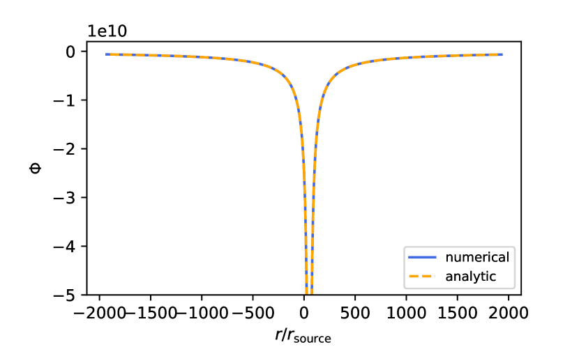
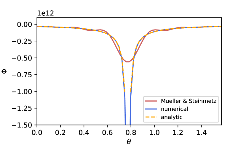
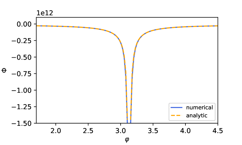
Figure 1.— Comparison of the analytic (dashed orange curves) and numerical (blue solid curves) solutions for the potential $\Phi$ of a point source at $r=5.46\times 10^{7}$, $\theta=0.246\pi$ and $\varphi=0.996\pi$ along the $r$-, $\theta$- and $\varphi$-coordinate lines through the source (top to bottom). In the middle panel, we also show the result of the algorithm of Müller & Steinmetz (1995) with a truncation point of $\ell_{\mathrm{max}}=25$ for the multipole expansion (red curve). In the top panel, the radial coordinate is measured relative to the radial coordinate $r_{\mathrm{source}}$ of the point mass.

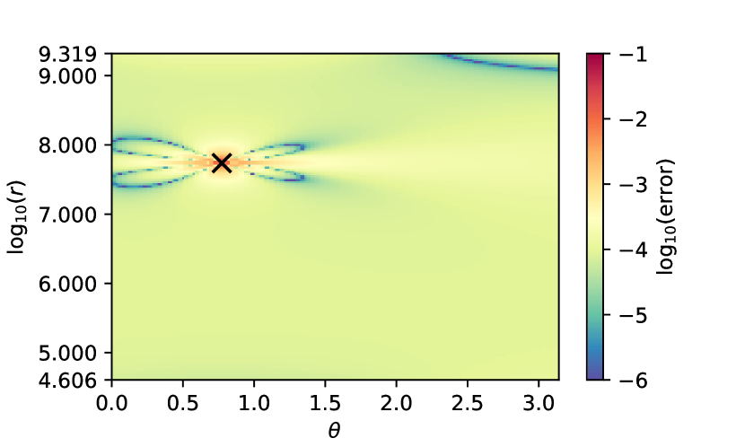
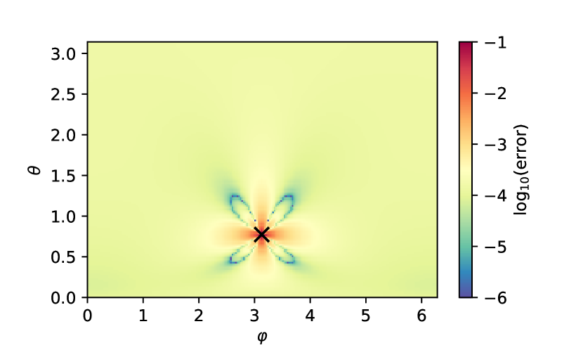
Figure 2.— Relative error of the numerical solution compared to the analytic solution on coordinate slices through the source with constant with constant $\varphi$ (left) and constant $r$ (right). The position of the point source is marked with a cross sign. Note that the numerical solution shows no visible artifacts at the grid axis ($\theta=0$ and $\theta=\pi$).

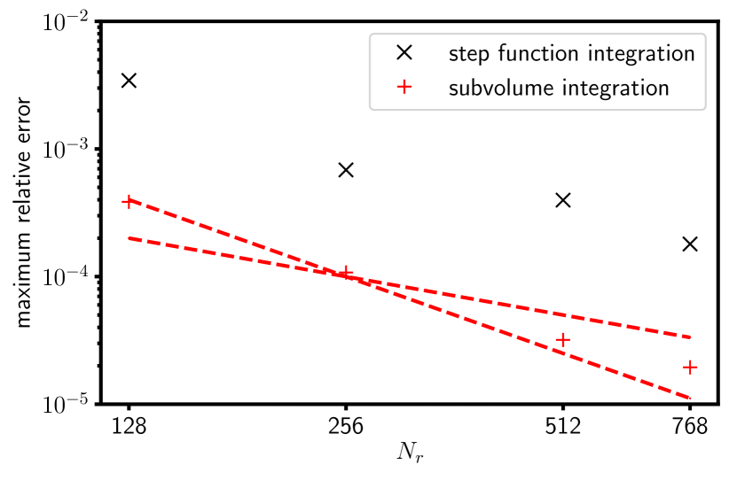
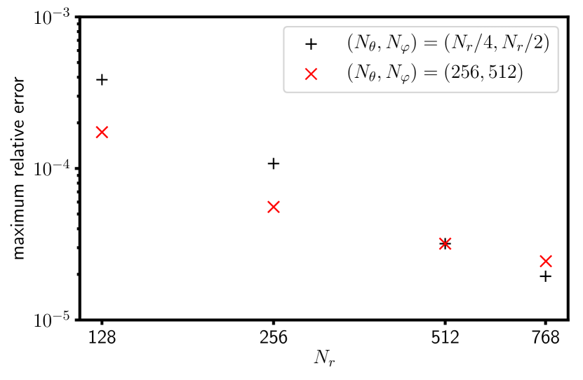
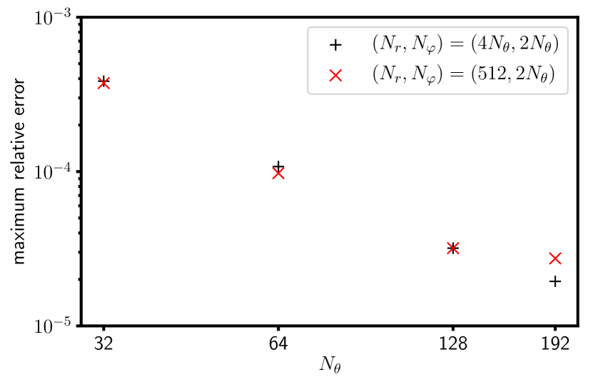
Figure 3.— Relative maximum error of the numerical solution for the case of a homogenous ellipsoid with $a=1$, $b=1.5$, and $c=2$. A uniform grid with an outer boundary of $r_{\mathrm{out}}=5$ is used in all cases. The top panel shows the error as a function of grid size using a constant ratio $N_{r}:N_{\theta}:N_{\varphi}=4:1:2$. The errors are larger if the mass per cell is evaluated using simple step function integration (black dots) and smaller by an order of magnitude if we use subvolume integration (red dots). The dashed red lines indicate power laws of $N_{r}^{-1}$ and $N_{r}^{-2}$. The middle panel compares the maximum error for varying $N_{r}$ using a constant ratio $N_{r}:N_{\theta}:N_{\varphi}=4:1:2$ (black) to solutions with varying $N_{r}$ and $N_{\theta}=128$ and $N_{\varphi}=512$ (red); subvolume integration is used in both cases. The bottom panel compares the maximum error for varying $N_{\theta}=N_{\varphi}/2$ using a constant ratio $N_{r}:N_{\theta}:N_{\varphi}=4:1:2$ (black) to a series with $N_{r}=512$ (red).

5. Verification

It is customary to gauge approximate solvers for the Poisson equation by comparing to analytic solutions for configurations with an extended density distribution, such as MacLaurin spheroids (Chandrasekhar, 1987) and various axisymmetric disk models (e.g. Kuzmin, 1956; Miyamoto & Nagai, 1975; Satoh, 1980).

5.1. Displaced Point Source

In our case, we can also consider a much more stringent test case, namely the field of a point source displaced from the origin of the grid. For code verification, we choose a grid with $550$ radial zones with constant spacing in $\log r$ from $r=10^{4}$ to $r=2.1\times 10^{9}$ (in non-dimensional units) and $128\times 256$ uniformly spaced zones zones in the $\theta$- and $\varphi$-direction. A mass of $m=1.352735\times 10^{18}$ is placed in the zone with indices $(i,j,k)=(366,32,128)$ or $r=5.46\times 10^{7}$, $\theta=0.246\pi$ and $\varphi=0.996\pi$; this choice corresponds to a density of $\rho=1$ in that zone.

Figure 1 compares the numerical solution to the analytic solution for a point source along three coordinate lines through the source, and Figure 2 shows the relative error on two surfaces with $\phi=\mathrm{const}.$ and $r=\mathrm{const}.$ that intersect the source location. Our solver tracks the analytic solution almost perfectly; even in the zones directly adjacent to the point source, the maximum relative error is only 10%. The Gibbs phenomenon that affects the truncated multipole solver of Müller & Steinmetz (1995) (middle panel of Figure 1) is completely eliminated. Although the Gibbs phenomenon is absent or much less pronounced in case of the truncated multipole expansion for smoother, more extended sources, one must bear in mind that the relative error in the potential (which is typically used for the verification of Poisson solvers; see Müller & Steinmetz, 1995; Couch et al., 2013; Almanstötter et al., 2018) can give a too favourable impression of the solution accuracy. When the solution is used to compute gravitational acceleration terms in a hydrodynamics code, it is the derivatives of the potential that matter, and these are much more severely affected by the Gibbs phenomenon of the multipole expansion than the potential itself.

5.2. Convergence – Potential of an Ellipsoid

Since the analytic solution for the potential of a point source is singular, this case is not well suited for studying the convergence of the algorithm. We therefore consider the potential of an ellipsoid (Chandrasekhar, 1987) to address the convergence properties of the scheme; i.e. we use a source density of the form

$$\rho=\left\{\begin{array}[]{ll}1,&\frac{x^{2}}{a^{2}}+\frac{y^{2}}{b^{2}}+\frac{z^{2}}{c^{2}}\leq 1\\ 0,&\mathrm{else}\end{array}\right..$$ (33)

The solution for $\Phi$ is given by (Chandrasekhar, 1987; Almanstötter et al., 2018)

$$\Phi=\pi abc\left(A(\mathbf{r})X^{2}+B(\mathbf{r})y^{2}+C(\mathbf{r})z^{2}-D(\mathbf{r})\right),$$ (34)

in terms of the integrals

$$A(\mathbf{r}) = \int\limits_{u}^{\infty}\left[(a^{2}+\lambda)^{3}(b^{2}+\lambda)(c^{2}+\lambda)\right]^{-1/2}\mathrm{d}\lambda,$$ (35)

$$B(\mathbf{r}) = \int\limits_{u}^{\infty}\left[(a^{2}+\lambda)(b^{2}+\lambda)^{3}(c^{2}+\lambda)\right]^{-1/2}\mathrm{d}\lambda,$$ (36)

$$C(\mathbf{r}) = \int\limits_{u}^{\infty}\left[(a^{2}+\lambda)(b^{2}+\lambda)(c^{2}+\lambda)^{3}\right]^{-1/2}\mathrm{d}\lambda,$$ (37)

$$D(\mathbf{r}) = \int\limits_{u}^{\infty}\left[(a^{2}+\lambda)(b^{2}+\lambda)(c^{2}+\lambda)\right]^{-1/2}\mathrm{d}\lambda.$$ (38)

Here $u$ is the real root of

$$\frac{x^{2}}{a^{2}+u}+\frac{y^{2}}{b^{2}+u}+\frac{z^{2}}{c^{2}+u}=1,$$ (39)

if $\mathbf{r}$ lies outside the spheroid, and $u=0$ otherwise. We choose an ellipsoid of the same shape as Almanstötter et al. (2018) with $a=1$, $b=1.5$, and $c=2$.

In Figure 3, we show the convergence of the solution – quantified by the maximum relative error – on a uniform grid in $r$ with an outer boundary of $r_{\mathrm{out}}=5$. When comparing the numerical and the analytic solution, we face two separate issues: We introduce errors by discretizing $\Phi$ and assuming constant source density within cells in a finite-volume approach according to Equations (9-12). Moreover, errors in the evaluation of the mass per cell and hence of the source density in Equation (9) will also degrade the solution. We deal with those two types of discretization error by computing the source in two ways. In the first approach, we use simple step-function integration and set $\rho=1$ or $\rho=0$ depending on whether the cell centre lies inside or outside the ellipsoid. In the second approach of subvolume integration, we recursively divide the original cell volume $\delta V$ into octants by halving the grid spacing in $r$, $\theta$, and $\varphi$ before applying step-function integration. The division into subvolumes is stopped if a refined cell either lies completely inside or outside the ellipsoid, or if its volumes is smaller than $10^{-6}\delta V$, where $\delta V$ is the volume of the parent cell on the original grid. In both cases, we vary the angular resolution from $N_{r}=128$ to $N_{r}=768$, keeping the ratio $N_{\varphi}/N_{r}=2N_{\theta}/N_{r}=1/2$ constant.

The top panel of Figure 3 shows that the evaluation of the source density completely dominates the error for this test problem. When the source density is evaluated accurately using subvolume integration, the error decreases slightly slower than $N_{r}^{-2}$. Since Almanstötter et al. (2018) do not specify whether they obtain the source density by step function integration or by a more accurate method, a direct comparison with their work using the truncated multipole expansion is difficult, but we note that we already obtain better accuracy for $N_{r}=512$ and $\delta_{\theta}=\delta_{\varphi}=1.4^{\circ}$ than in their high-resolution case with $N_{r}=800$ and $\delta_{\theta}=\delta_{\varphi}=1^{\circ}$.

The radial and angular resolution are not always of equal importance for the solution error. In the middle and bottom panels of Figure 3, we also show the maximum relative error for cases with varying $N_{r}$ and constant $N_{\theta}=128$ and $N_{\varphi}=256$ (middle panel) and with varying $N_{\theta}=N_{\varphi}/2$ and constant $N_{r}=512$. For this particular problem, decreasing angular resolution with respect to our baseline case of $(N_{r},N_{\theta},N_{\varphi})=(512,128,256)$ appears to be much more problematic than decreasing radial resolution.

We also investigate whether the solution accuracy is strongly sensitive to local variations in the radial grid resolution. Still using subvolume integration, we solve the Poisson equation on a grid with a resolution of $(N_{r},N_{\theta},N_{\varphi})=(512,128,256)$. We choose the radial grid to be identical to the uniform grid used before up to $r=1.5$ and maintain constant $\delta r/r$ outside, so that the outer boundary is at $r_{\mathrm{out}}=48.7$. This actually decreases the maximum relative error from $3.2\times 10^{-5}$ in the baseline model to $2.7\times 10^{-5}$. We also considered a jump in grid resolution with a sudden increase of the (otherwise uniform) grid spacing $\delta r$ by $50\%$ outside $r=1.5$, which increases the maximum error slightly to $3.6\times 10^{-5}$. This suggests that the algorithm deals well with variations in grid spacing that are not too extreme.

6. Conclusions

We have presented an exact, non-iterative solver for the Poisson equation on spherical polar grids. Compared to the truncated multipole expansion (Müller & Steinmetz, 1995) used in many astrophysical simulation codes based on spherical polar coordinates, our method has a number of attractive features. Solving the discretized Poisson equation exactly allows one to implement the gravitational momentum and energy source terms in a fully conservative manner, and ensures well-behaved convergence with increasing grid resolution. The method also adroitly handles off-centred mass distributions without the need to move the center of the spherical harmonics expansion (Couch et al., 2013), and even multiple density concentrations are not an obstacle. This comes at little extra cost, since the operation count of the algorithm is competitive with the standard multipole expansion for $N_{\ell}=10\ldots 20$ for typical 3D grid setups. The parallel performance is sufficient for the algorithm to be used in hydrodynamical simulations at least on a few hundreds of cores. Further optimization of the parallel algorithm may still be possible, e.g. by exploiting symmetries in the FFT for real input data to reduce the communication volume. We make a Fortran implementation of the serial algorithm and an easily adaptable template of an MPI parallel version available under https://doi.org/10.5281/zenodo.1442635.

Although the method presented here is both accurate and efficient, it comes with less flexibility in the choice of the grid setup than the standard multipole expansion. The parallel code currently requires the dimension of the $\theta$- and $\varphi$- grid to be a power of two. This, however, is not a fundamental restriction and could be remedied by using more general algorithms for the parallel FFT and matrix-vector multiplication. A more serious limitation is that the algorithm cannot readily be generalized to overset spherical grids (Kageyama & Sato, 2004; Wongwathanarat et al., 2010) or spherical grids with non-orthogonal patches like the cubed-sphere grid (Wongwathanarat et al., 2016). One option would be to map to an auxiliary global spherical polar grid for the Poisson solver. In a distributed-memory paradigm, the amount of data that needs to be communicated between tasks would only be $\mathcal{O}(4N_{r}N_{\theta}N_{\varphi})$ for bilinear interpolation, which would not increase MPI traffic tremendously. On the downside, the mapped solution would no longer fulfill the discretized finite-volume form of the Poisson equation exactly on the original grid, and hence a major advantage of the algorithm would be lost.

There are, however, alternative solutions for some of the problems that prompt the use of multi-patch grids or non-orthogonal spherical grids in the first place. The problem of stringent CFL time step constraints near the grid axis can also be solved or mitigated by filtering schemes (Müller, 2015) or non-uniform spacing in the $\theta$-direction, which our new method can easily accommodate. In the future, we will investigate whether further refinements of these techniques can also reduce other shortcomings of spherical polar grids such as flow artifacts near the axis.

Appendix A Non-Orthonormality of Standard Multipole Expansion

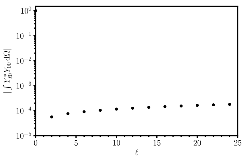
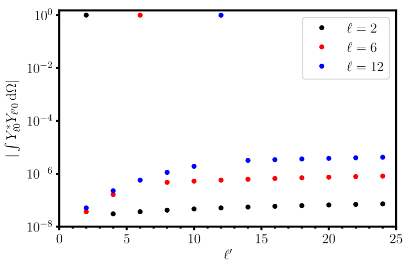
Figure 4.— Left: Overlap between $Y_{00}$ and spherical harmonics of even $\ell$ and $m=0$ for the cell-centred evaluation of spherical harmonics in the overlap integral in Equation (A2) in case of a uniform grid in $\theta$ with 128 zones. Right: Overlap between $Y_{2,0}$ (black), $Y_{6,0}$ (red), and $Y_{12,0}$ (blue) and other spherical harmonics of even $\ell^{\prime}$ and $m=0$ evaluated using the method of Müller & Steinmetz (1995), again for a uniform grid in $\theta$ with 128 zones.

The use of standard spherical harmonics in the multipole expansion of the Green’s function (Equation 2) can lead to solution artifacts and divergence problems if too many terms in the multipole expansion are retained. While some of these problems can be eliminated by using analytic integrals of spherical harmonics (Müller & Steinmetz, 1995) or by staggering the grids for the density and the potential (Couch et al., 2013), other problems are related to the failure of these methods to respect the orthogonality relation

$$\int Y^{*}_{\ell m}Y_{\ell^{\prime}m^{\prime}}\,\mathrm{d}\Omega=\delta_{\ell\ell^{\prime}}\delta_{mm^{\prime}}.$$ (A1)

Let us consider the simplest method for decomposing the source density into spherical harmonics in Equation (8). If we already write the source density as $\rho(r,\theta,\varphi)=\sum_{\ell,m}c_{\ell m}(r)Y_{\ell m}(\theta,\varphi)$, and evaluate the overlap integral using cell-centred values for the spherical harmonics as in Couch et al. (2013), we obtain terms of the form

$$D_{\ell\ell,mm^{\prime}}=\sum_{j,k}Y^{*}_{\ell m}(\theta_{j},\varphi_{k})Y_{\ell m}(\theta_{j},\varphi_{k})\Delta\Omega_{j,k},$$ (A2)

where $\Delta\Omega_{j,k}$ is the solid angle occupied by a single cell. In general, we will find $D_{\ell\ell,mm^{\prime}}\neq\delta_{\ell\ell^{\prime}}\delta_{mm^{\prime}}$, so that any multipole in the source gives rise to other spurious multipoles in the solution. It is particularly problematic that even the monopole $Y_{00}$ overlaps with all other spherical harmonics with even $\ell$ and $m=0$ as illustrated in the left panel of Figure 4. Thus, the solution does not preserve spherical symmetry. Moreover, the coefficients of the spurious multipoles tend to be correlated so that they manifest themselves as small spikes near the axis that grow and become narrower with larger $N_{\ell}$. Whether or not the solution is evaluated at cell centers or cell interfaces does not change this behavior. The straightforward cell-centred evaluation of spherical harmonics in the overlap integral is therefore inadvisable in spherical polar coordinates, although it remains the only practical approach in Cartesian coordinates.

The alternative approach of Müller & Steinmetz (1995) merely assumes constant source density within cells and then evaluates the integrals over spherical harmonics analytically. This is tantamount to replacing $Y_{\ell m}(\theta_{j},\varphi_{k})$ with its cell average $\hat{Y}_{\ell m,jk}$,

$$Y_{\ell m}(\theta_{j},\varphi_{k})\rightarrow\hat{Y}_{\ell m,jk}=\frac{1}{\Delta\Omega_{j,k}}\int\limits_{\theta_{j-1/2}}^{\theta_{j+1/2}}\int\limits_{\varphi_{k-1/2}}^{\varphi_{k+1/2}}Y_{\ell m}(\theta,\varphi)\sin\theta\,\,\mathrm{d}\varphi\,\mathrm{d}\theta$$ (A3)

in Equation (A2). This ensures that overlap integrals with $Y_{00}$ reduce to their correct analytic value so that $D_{\ell 0,m0}=\delta_{\ell 0}\delta_{m0}$ and the solution remains spherically symmetric if the source density is. However, the spurious overlap between higher multipoles is not eliminated as shown in the right panel of Figure 4. However, contrary to the naive step-function integration, the spurious multipoles do not pose serious problems for moderately large values of the maximum multipole number $N_{\ell}$ in practice.

References

- Almanstötter et al. (2018) Almanstötter, M., Melson, T., Janka, H.-T., & Müller, E. 2018, ApJ, 863, 142
- Anderson et al. (1999) Anderson, E., et al. 1999, LAPACK Users’ Guide, 3rd edn. (Philadelphia, PA: Society for Industrial and Applied Mathematics)
- Barnes & Hut (1986) Barnes, J., & Hut, P. 1986, Nature, 324, 446
- Batchelor (1953) Batchelor, G. K. 1953, Quarterly Journal of the Royal Meteorological Society, 79, 224
- Blackford et al. (2002) Blackford, S., et al. 2002, ACM Trans. Math. Softw., 28, 135
- Brackbill & Barnes (1980) Brackbill, J. U., & Barnes, D. C. 1980, Journal of Computational Physics, 35, 426
- Brandt (1977) Brandt, A. 1977, Mathematics of Computation, 31, 333
- Bruenn et al. (2013) Bruenn, S. W., et al. 2013, ApJ, 767, L6
- Burrows et al. (2018) Burrows, A., Vartanyan, D., Dolence, J. C., Skinner, M. A., & Radice, D. 2018, Space Science Reviews, 214, 33
- Chandrasekhar (1987) Chandrasekhar, S. 1987, Ellipsoidal figures of equilibrium (New York: Dover)
- Chen et al. (2000) Chen, H., Su, Y., & Shizgal, B. D. 2000, Journal of Computational Physics, 160, 453
- Choi et al. (1995) Choi, J., et al. 1995, ScaLAPACK: A Portable Linear Algebra Library for Distributed Memory Computers — Design Issues and Performance, LAPACK Working Note 95
- Cordero-Carrión et al. (2009) Cordero-Carrión, I., Cerdá-Durán, P., Dimmelmeier, H., Jaramillo, J. L., Novak, J., & Gourgoulhon, E. 2009, Phys. Rev. D, 79, 024017
- Couch et al. (2013) Couch, S. M., Graziani, C., & Flocke, N. 2013, ApJ, 778, 181
- Eastwood & Brownrigg (1979) Eastwood, J. W., & Brownrigg, D. R. K. 1979, Journal of Computational Physics, 32, 24
- Eleftheriou et al. (2005) Eleftheriou, M., Fitch, B., Rayshubskiy, A., Ward, T. J. C., & Germain, R. 2005, in Euro-Par 2005 Parallel Processing. Euro-Par 2005. Lecture Notes in Computer Science, ed. J. C. Cunha, P. D. Medeiros, & D. W. Hobill, Vol. 3648 (Berlin: Springer), 795–803
- Fornberg (1995) Fornberg, B. 1995, SIAM J. Sci. Comput., 16, 1071
- Frigo & Johnson (2005) Frigo, M., & Johnson, S. G. 2005, Proceedings of the IEEE, 93, 216, special issue on “Program Generation, Optimization, and Platform Adaptation”
- Fryxell et al. (2000) Fryxell, B. A., et al. 2000, ApJS, 131, 273
- Hockney (1965) Hockney, R. W. 1965, Journal of the ACM, 12, 95
- Jacobson (1999) Jacobson, M. Z. 1999, Fundamentals of Atmospheric Modeling, 2nd edn. (Cambridge University Press), 828
- Kageyama & Sato (2004) Kageyama, A., & Sato, T. 2004, Geochemistry, Geophysics, Geosystems, 5, n/a, q09005
- Kuzmin (1956) Kuzmin, G. G. 1956, Astronomicheskii Zhurnal, 33, 27
- Lai & Wang (2002) Lai, M.-C., & Wang, W.-C. 2002, Numerical Methods for Partial Differential Equations, 18, 56
- LeVeque (1998) LeVeque, R. J. 1998, in Saas-Fee Advanced Course 27: Computational Methods for Astrophysical Fluid Flow. (Berlin: Springer), 1–159
- Liebendörfer et al. (2009) Liebendörfer, M., Whitehouse, S. C., & Fischer, T. 2009, ApJ, 698, 1174
- Livne et al. (2004) Livne, E., Burrows, A., Walder, R., Lichtenstadt, I., & Thompson, T. A. 2004, ApJ, 609, 277
- Marek & Janka (2009) Marek, A., & Janka, H. 2009, ApJ, 694, 664
- Miyamoto & Nagai (1975) Miyamoto, M., & Nagai, R. 1975, PASJ, 27, 533
- Müller (2015) Müller, B. 2015, MNRAS, 453, 287
- Müller et al. (2010) Müller, B., Janka, H., & Dimmelmeier, H. 2010, ApJS, 189, 104
- Müller & Janka (2015) Müller, B., & Janka, H.-T. 2015, MNRAS, 448, 2141
- Müller & Steinmetz (1995) Müller, E., & Steinmetz, M. 1995, Computer Physics Communications, 89, 45
- Obergaulinger et al. (2006) Obergaulinger, M., Aloy, M. A., & Müller, E. 2006, A&A, 450, 1107
- Ogura & Phillips (1962) Ogura, Y., & Phillips, N. A. 1962, Journal of Atmospheric Sciences, 19, 173
- Satoh (1980) Satoh, C. 1980, PASJ, 32, 41
- Shu (1992) Shu, F. H. 1992, Physics of Astrophysics, Vol. II (University Science Books)
- Weatherford et al. (2005) Weatherford, C., Red, E., & Hoggan, P. 2005, Molecular Physics, 103, 2169
- Wongwathanarat et al. (2016) Wongwathanarat, A., Grimm-Strele, H., & Müller, E. 2016, A&A, 595, A41
- Wongwathanarat et al. (2010) Wongwathanarat, A., Hammer, N. J., & Müller, E. 2010, A&A, 514, A48