Spectral Functions of One-dimensional Systems with Correlated Disorder

Abstract

We investigate the spectral function of Bloch states in an one-dimensional tight-binding non-interacting chain with two different models of static correlated disorder, at zero temperature. We report numerical calculations of the single-particle spectral function based on the Kernel Polynomial Method, which has an $\mathcal{O}(N)$ computational complexity. These results are then confirmed by analytical calculations, where precise conditions were obtained for the appearance of a classical limit in a single-band lattice system. Spatial correlations in the disordered potential give rise to non-perturbative spectral functions shaped as the probability distribution of the random on-site energies, even at low disorder strengths. In the case of disordered potentials with an algebraic power-spectrum, $\propto\left|k\right|^{-\alpha}$, we show that the spectral function is not self-averaging for $\alpha\geq 1$.

1 Introduction

The one-electron spectral function is a key ingredient in the understanding of interacting and of disordered electronic systems. It can be thought of as the energy distribution of a state of momentum $\mathbf{k}$, $\rho(\mathbf{k},E)$. In a non-interacting translationally invariant system it is simply a Dirac delta function of energy, peaked at the single particle energy $E_{\mathbf{k}}$.

The spectral function has been the subject of intense study in correlated electronic systems, because it bears clear signatures of the low energy phases of interacting electron systems, whether it be a Fermi Liquid[3, 2], a marginal Fermi liquid as in high $T_{c}$ cuprates [1], or a one-dimensional Tomonaga-Luttinger liquid, with charge-spin separation [8]. It is experimentally accessible by angle-resolved photo-emission spectroscopy (ARPES) [5, 12].

Random disorder can introduce a finite width on the spectral function, averaged over disorder realizations, even in the absence of interactions. The more common approaches to its calculation rely on the Born approximation for the decay rate of a momentum state due to scattering by the disordered potential. They implicitly (or explicitly) assume that the disordered potential is a weak perturbation of the kinetic or band energy terms of the Hamiltonian, and generally lead to a lorentzian line shape for $\rho(\mathbf{k},E)$. One does not need strong disorder to ensure localization in 1D or 2D, and in weak localization this approach to the one particle spectral function is quite sufficient [16].

The concept of spectral function, however, is not confined to weak disorder. Very efficient numerical methods are able to compute $\rho(\mathbf{k},E)$ for any strength of disorder [26]. Trappe, Delande and Muller[23] studied a continuum model with correlated disorder and argued that when the root mean square of the local random potential far exceeds the kinetic energy scale, $E_{\xi}=\hbar^{2}/2m\xi^{2}$ (where $\xi$ is the spatial correlation length of the disorder), the non-commutativity of position and momentum can be ignored, and a classical limit is achieved, in which the spectral function portrays the probability distribution of the random potential. The coherent potential approximation, a well-known approximation to treat disorder problems [21, 24], which in its original formulation cannot account for spatially correlated disorder, has been generalized to treat spatially correlated disorder[27] and can also go beyond perturbation theory and reproduce the classical limit results for strong disorder.

The exquisite control that has become available in ultra cold atom experiments has renewed interest in the experimental study of disordered potentials, free of the complication of interactions, always present in electronic systems. Atomic clouds can be transferred into a random potential created by laser speckle and several experiments have been made on Anderson localization[15, 13, 10], included a measurement of the dependence of the mobility edge with the strength of the disordered potential[19].

The random potential implemented in ultra-cold atom experiments is correlated in space, in contrast with the standard Anderson model of site disorder. Disorder correlation studies of Anderson localization have been carried out for several decades now [11]. Significant results were obtained in 1D, where it was found that extended states can exist at discrete energies in short-range correlated models [7] and that a mobility edge appears in models with power-law decay of spatial correlation of the random potential [9, 6].

Quite recently, a direct measurement of the one-particle spectral function in an ultra-cold atom experiment was reported[25]. By varying the intensity of the random potential, one observes a change from a perturbative lorentzian shape, to an asymmetric line shape, that reflects the probability distribution of the random potential.

Our focus in this paper is also on the spectral function in 1D tight-binding models with correlated disorder. Unlike in the continuum case, band models have an intrinsic kinetic energy scale given by the bandwidth. It is relevant to consider whether the classical limit can be reached even when disorder is weak, in the sense that the mean free path is much larger than the lattice spacing. When the disorder correlation length is much larger than the unit cell, scattering becomes local in momentum-space and we explore this feature to show analytically how the classical limit emerges. Moreover, we also study the interesting case of disorder correlations that decay as a power-law, with a characteristic power spectrum $S\left(k\right)\sim 1/k^{\alpha}$ [6]. This type of disorder has an infinite correlation length, and would appear to be always in the classical limit. Instead, we find that this limit for the averaged spectral function requires that $\alpha>1$, when the scattering really becomes local in momentum space. Our results are confirmed by numerical calculations.

Localization properties have been studied for these power-law spectrum disorder models. While in the Anderson and other short-range correlated models, all states are localized in 1D, for these power-law spectrum models it has been claimed that a mobility edge appears for $\alpha\geq 2$[6]. This conclusion has been contested, on the grounds that in the thermodynamic limit this potential is not really disordered[17]. To investigate possible issues with the thermodynamic limit for these models, we investigated the statistical properties of the spectral function for different sized chains. We did find a transition from self-averaging to non self-averaging behavior at $\alpha=1$. The spectral function of even a very a large system will depend on the specific realization of disorder it carries. It is significant, however, that this transition occurs well below the value of $\alpha=2$. The spectral function remains non self-averaging beyond $\alpha=2$, which makes it hard to argue that the potential is not really disordered.

The rest of this paper is organized as follows. In the next section, we start by defining our basic tight-binding model. Randomness is introduced in the site energies, and is characterized by its Fourier components, which have a prescribed magnitude, but randomly distributed independent phases. We then briefly review the Kernel Polynomial Method (KPM) as a tool for the numerical calculation of the spectral function. In section III, we present our numerical results for $\rho\left(k,E\right)$, and confirm our main findings by analytical calculations done in Section IV. Additionally, some numerical results of the fluctuations of $\rho(k,E)$ and its self-averaging properties are also discussed. Finally, in Section V we sum up our conclusions.

2 The Disorder Model and The Kernel Polynomial Method

2.1 The Disorder Model

The Hamiltonian we use is an one-dimensional tight-binding model with nearest neighbor hopping and random site energies,

$$\mathcal{H}=\sum_{m=0}^{L-1}\varepsilon_{m}\left|\varphi_{m}\right\rangle\left\langle\varphi_{m}\right|-t\left[\sum_{m=0}^{L-1}\left|\varphi_{m+1}\right\rangle\left\langle\varphi_{m}\right|+\left|\varphi_{m}\right\rangle\left\langle\varphi_{m+1}\right|\right]$$ (1)

where $\left\{\left|\varphi_{m}\right\rangle;\,m=0,\dots,L-1\right\}$ are the local Wannier states. In what follows, we impose periodic boundary conditions by setting $\left|\varphi_{m}\right\rangle=\left|\varphi_{m+N}\right\rangle$, the lattice parameter $a$ is taken as $1$, and all energies are measured in units of the hopping $t$ (i.e., $t=1$).

If there were no disorder, the exact eigenstates of the previous Hamiltonian would be the Bloch states, defined as

$$\left|k\right\rangle=\frac{1}{\sqrt{L}}\sum_{m=0}^{L-1}e^{ikm}\left|\varphi_{m}\right\rangle.$$ (2)

The presence of static disorder causes scattering of $\left|k\right\rangle\to\text{$\left|k+q\right\rangle$}$, characterized by the matrix elements of the random potential $\mathcal{V}:=\sum_{m}\varepsilon_{m}\left|\varphi_{m}\right\rangle\left\langle\varphi_{m}\right|$ that connect two Bloch states, i.e.,

$$\left\langle k+q\right|\mathcal{V}\left|k\right\rangle=\frac{1}{L}\sum_{m}\varepsilon_{m}e^{-iqm},$$ (3)

seen here to depend only on the transferred momentum $q$. We easily invert Eq. 3 to express the local energies as the Fourier sum

$$\varepsilon_{m}=\sum_{q}\left\langle k+q\right|\mathcal{V}\left|k\right\rangle e^{iqm}.$$ (4)

For the purposes of this paper, we choose to model the randomness by taking these matrix elements as

$$\left\langle k+q\right|\mathcal{V}\left|k\right\rangle=V(q)e^{i\phi_{q}},$$ (5)

where $V(q):=\left|\left\langle k+q\right|\mathcal{V}\left|k\right\rangle\right|$ is a specified even function of $q$ and $\phi_{q}$ is a random phase with a uniform probability distribution in the circle $\left[0,2\pi\right[$. The different phases are independent variables except for the constraints $\phi_{q}=-\phi_{-q}$, which ensure the hermiticity of the Hamiltonian. With these definitions, the mean of the site energies is $\overline{\varepsilon_{m}}=\sum_{q}V(q)\overline{e^{i\phi_{q}}}e^{iqm}=V(0)$, since the condition $\phi_{q}=-\phi_{-q}$ fixes $\phi_{0}=0$ and the individual phase averages are zero otherwise, $\overline{e^{i\phi_{q}}}=\delta_{q,0}$. As $\overline{\varepsilon_{m}}$ merely shifts the spectrum, we will always choose $\overline{\varepsilon_{m}}=0$, meaning that $V(0)=0$.

In general, the values of the energies in different sites will be correlated in this model of disorder. The two-site covariance of the potential can be written as

$$\overline{\varepsilon_{n}\varepsilon_{m}}=\sum_{q,q^{\prime}\neq 0}V(q)V(q^{\prime})\overline{e^{i\phi_{q^{\prime}}}e^{i\phi_{q}}}e^{i\left(qm+q^{\prime}n\right)},$$ (6)

where all the phase averages factorize (unless $q=-q^{\prime}$) and the average of a single phase is zero,

$$\overline{e^{i\phi_{q}}} =0,$$ (7a)

$$\overline{e^{i\phi_{q^{\prime}}}e^{i\phi_{q}}} =\delta_{q+q^{\prime},0}.$$ (7b)

Hence (using the property $V(q)=V(-q)$)

$$\overline{\varepsilon_{n}\varepsilon_{m}}=2\sum_{q>0}V^{2}(q)\cos\left(q(n-m)\right).$$ (8)

From Eq. 8, we see that $V^{2}(q)$ can be related to the Fourier transform of the spatial correlation function $C\left(n\right)$ of the disordered potential, as follows

$$V^{2}(q):=\frac{1}{L}\sum_{n}\overline{\varepsilon_{n}\varepsilon_{0}}e^{iqn}=\frac{1}{L}\sum_{n}C\left(n\right)e^{iqn}.$$ (9)

In the case of an uncorrelated disorder, like in the usual Anderson’s model, we have

$$\overline{\varepsilon_{n}\varepsilon_{m}}=\sigma_{\varepsilon}^{2}\delta_{n,m},$$ (10)

with $\sigma_{\varepsilon}^{2}:=\overline{\varepsilon^{2}}$, or, equivalently

$$V^{2}\left(q\right)=\frac{1}{L}\sigma_{\varepsilon}^{2}.$$ (11)

Thus, for these models, the magnitude of the scattering matrix element from $k\to k+q$ is independent of the transferred momentum, $q$ .

2.1.1 Gaussian Correlated Disorder

Our first model of correlated disorder is the gaussian case. For that, we choose

$$V(q):=\frac{A(q_{c})}{\sqrt{L}}\exp\left(-q^{2}/4q_{c}^{2}\right),$$ (12)

where $A(q_{c})$ is a measure for the strength of disorder. The $L^{-\frac{1}{2}}$ factor in Eq.12 is introduced in order to have a well-defined thermodynamic limit for the local variance and correlation functions of the disordered potential.

In this model, the values of $V(q)$ are only significant inside an interval of linear size $q_{c}$, centered around $q=0$. This means that the disordered potential couples Bloch states with nearby momenta, more strongly. The statistical properties of the corresponding potential in the $L\rightarrow\infty$ limit, can be calculated through Eq. 8, yielding

$$\overline{\varepsilon^{2}}=\sigma_{\epsilon}^{2}= A^{2}(q_{c})\int_{-\pi}^{\pi}\frac{dq}{2\pi}e^{-q^{2}/2q_{c}^{2}},$$ (13a)

$$\overline{\varepsilon_{n}\varepsilon_{m}}=A^{2}(q_{c}) \int_{-\pi}^{\pi}\frac{dq}{2\pi}e^{-q^{2}/2q_{c}^{2}}e^{iq(n-m)}.$$ (13b)

From these two equations, we notice that the normalized correlation function does not depend on the parameter $A(q_{c})$, i.e.

$$\Gamma(n-m):=\frac{\overline{\varepsilon_{n}\varepsilon_{m}}}{\sigma_{\varepsilon}^{2}}=\frac{\int_{-\pi}^{\pi}\frac{dq}{2\pi}e^{-q^{2}/2q_{c}^{2}}e^{iq(n-m)}}{\int_{-\pi}^{\pi}\frac{dq}{2\pi}e^{-q^{2}/2q_{c}^{2}}}.$$ (14)

Finally, all the integrals above can be done analytically in the limit when $q_{c}\ll\pi$. In this case, the integration intervals may be extended to $k\in\left]-\infty,+\infty\right[$ and we get,

$$\Gamma(m)=\exp\left(-\frac{q_{c}^{2}m^{2}}{2}\right).$$ (15)

The correlation function of site energies is gaussian in real space with a decay length $\xi=q_{c}^{-1}$. In this same limit, we can also relate the parameter $A(q_{c})$ with the local disorder strength using Eq. 13a, i.e.

$$A^{2}(q_{c})=\sqrt{2\pi}\frac{\sigma_{\varepsilon}^{2}}{q_{c}},$$ (16)

meaning that,

$$V(q)=\left(2\pi\right)^{\frac{1}{4}}\frac{\sigma_{\varepsilon}}{\sqrt{q_{c}L}}\exp\left(-q^{2}/4q_{c}^{2}\right).$$ (17)

2.1.2 Power-Law Correlated Disorder

For our second model of disorder, we take the power-law potential defined by De Moura and Lyra[6], for a periodic chain of $L$ sites, as

$$\varepsilon_{m}=2A(\alpha)\sum_{p=1}^{L/2}\left(\frac{2\pi}{L}\right)^{\frac{1-\alpha}{2}}\frac{1}{p^{\frac{\alpha}{2}}}\cos\left(\frac{2\pi mp}{L}+\phi_{p}\right).$$ (18)

The phases $\phi_{p}$ have the same properties as before, being uniformly distributed in $\left[0,2\pi\right[$. We can reduce this definition to our formulation by writing the Bloch wave-numbers as

$$q:=\frac{2\pi}{L}p,$$ (19)

so that Eq. 18 becomes

$$\varepsilon_{m}=2A(\alpha)\left(\frac{2\pi}{L}\right)^{\frac{1}{2}}\sum_{q>0}\frac{1}{q^{\alpha/2}}\cos\left(qm+\phi_{q}\right).$$ (20)

Since this sum is carried only over the positive half of the first Brillouin zone (i.e., $q=2\pi p/L$, $p=1,\dots L/2$), it can be rewritten as

$$\varepsilon_{m} =\sum_{q\neq 0}V(q)e^{i\phi_{q}}e^{iqm},$$ (21)

with $V(q)$ defined as

$$V(q)=A(\alpha)\left(\frac{2\pi}{L}\right)^{\frac{1}{2}}\frac{1}{\left|q\right|^{\frac{\alpha}{2}}},$$ (22)

and the independent random phases obeying the constraint $\phi_{q}=-\phi_{-q}$. The $q=0$ term is excluded as before, and we have introduced a normalization factor $A(\alpha)$ that will define a finite variance for the local disorder.

To study the thermodynamic limit ($L\to\infty$) in the previous case (gaussian), we replaced all the sums over $q$ by integrals. In this case, since $q=2\pi p/L$, $p\in\mathbb{Z}\setminus\left\{0\right\},$ we could try to do the same, but this turns out to be quite tricky due to the possibility of generating low-$q$ singularities. Consider, as an example, the calculation of the disorder’s local variance,

$$\sigma_{\varepsilon}^{2}=\sum_{q\neq 0}V^{2}\left(q\right)=A^{2}(\alpha)\left(\frac{2\pi}{L}\right)\sum_{q\neq 0}\frac{1}{\left|q\right|^{\alpha}},$$ (23)

for $\alpha<1,$ the corresponding integral does not have a low-$q$ singularity and the situation is be very similar to a system with uncorrelated disorder. A more interesting case happens for $\alpha>1$, where the integrals will have low-$q$ singularities with a natural cut-off of $2\pi/L$. At the same time, in this case, the corresponding sum over $p$ in

$$\sigma_{\varepsilon}^{2}=2A^{2}(\alpha)\left(\frac{2\pi}{L}\right)^{1-\alpha}\sum_{p=1}^{L/2}\frac{1}{p^{\alpha}},$$ (24)

is found to converge as $L\to\infty$. These two facts mean that, no matter how large $L$ is, the number of terms contributing to the sum is always of $\mathcal{O}(1)$. Hence, we can never approximate it by an integral. Luckily, the infinite sum in Eq. 24 is known to define the Riemann Zeta function[22],

$$\sum_{p=1}^{\infty}\frac{1}{p^{\alpha}}:=\mathcal{\zeta}(\alpha).$$ (25)

Finally, in the same limit, the local variance of the disorder can be written as

$$\sigma_{\varepsilon}^{2}=2A^{2}(\alpha)\left(\frac{2\pi}{L}\right)^{1-\alpha}\zeta(\alpha),$$ (26)

allowing us to express $A^{2}(\alpha)$ in terms of $\sigma_{\varepsilon}$, as follows,

$$A^{2}(\alpha)=\frac{\sigma_{\varepsilon}^{2}}{2\mathcal{\zeta}(\alpha)}\left(\frac{2\pi}{L}\right)^{\alpha-1}.$$ (27)

The correlation function of this potential can also be calculated using,

$$\overline{\varepsilon_{n}\varepsilon_{m}} =\sum_{q\neq 0}V^{2}(q)e^{iq\left(n-m\right)}=\frac{4\pi A^{2}(\alpha)}{L}\sum_{q>0}\frac{1}{\left|q\right|^{\alpha}}\cos\left(q(n-m)\right).$$

Writing $q=2\pi p/L$ and taking the thermodynamic limit in the last sum, we can express the result in terms of a polylogarithm function [22, 17], $Li_{\alpha}(z):=\sum_{p=1}^{\infty}z^{p}/p^{\alpha}$, as follows,

$$\Gamma_{\alpha}(m)=\frac{\overline{\varepsilon_{0}\varepsilon_{m}}}{\sigma_{\varepsilon}^{2}}=\frac{1}{\mathcal{\zeta}(\alpha)}Re\left[Li_{\alpha}\left(e^{-\frac{2\pi im}{L}}\right)\right].$$ (28)

A plot of this space correlation function is shown in the Figure 1, for several values of the exponent $\alpha$[17].

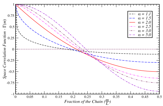
Figure 1: Plot of the space correlation for the power-law disordered potential as a function, calculated for several values of the exponent $\alpha$. The $\alpha\rightarrow+\infty$ limit yields a perfect cosine function, corresponding to an ordered system with an applied modulated potential.[17]

As a last remark, we note that to ensure a finite local variance, $\sigma_{\varepsilon}$, we had to choose $A^{2}(\alpha)\propto 1/L^{\alpha-1}$ (see Eq. 27). This weird fact implies that $A^{2}(\alpha)\to 0$, as $L\to\infty$ (for $\alpha>1$), which will have important consequences in what follows.

2.2 The Kernel Polynomial Method

The spectral function of a large disordered quantum system can be efficiently computed by a polynomial expansion-based technique — the Kernel Polynomial Method (KPM) [20, 18, 26, 14, 4]. In this approach, a function of an operator with spectrum normalized to the interval $\left]-1,1\right[$ is approximated by a truncated Chebyshev series. The expansion coefficients can be computed either by the stochastic evaluation of a trace [26, 14] or by the expectation values of Chebyshev polynomials in a given basis. Furthermore, the accuracy and numerical convergence of the KPM estimates are controlled by employing an optimized Gibbs damping factor and using sufficient number of Chebyshev polynomials [26]. The Chebyshev polynomial of the first kind, $T_{n}(x)$, is an $n^{th}$-degree polynomial in $x$, defined as

$$T_{n}(x)=\cos(n\,\arccos(x)),\quad n\in\mathbb{N}$$ (29)

where $x$ takes values in the interval $]-1,1[$. Moreover, the $T_{n}(x)$’s are generated by the following recurrence relations

$$T_{0}(x) =1,\,\,\,\,\,\,T_{1}(x)=x,$$ (30a)

$$T_{n+1}(x) =2xT_{n}(x)-T_{n-1}(x),$$ (30b)

and also satisfy the orthogonality relation

$$\int_{-1}^{1}\,T_{n}(x)T_{m}(x)(1-x^{2})^{-1/2}dx=\frac{\pi}{2}\delta_{n,m}(\delta_{n,0}+1).$$ (31)

In our case, we consider a free electron gas hopping on a finite cyclic chain of size $L$, under the influence of on-site correlated disorder. Suppose that the $L\times L$ Hamiltonian matrix $\mathcal{H}$ (Eq. 1), has eigenvalues $E_{\beta}$ with corresponding eigenstates $\left|\Psi_{\beta}\right\rangle$. Then its zero temperature spectral function has the form

$$\rho(k,E)=\sum_{\beta=0}^{L-1}\left|\left\langle k|\Psi_{\beta}\right\rangle\right|^{2}\delta(E-E_{\beta}),$$ (32)

where $\left|k\right\rangle$ is a Bloch state of one electron as defined in last section. Notice also that, in the absence of disorder $\rho(k,E)=\delta(E-E_{k})$, and by summing $\rho(k,E)$ over $k$ one obtains the density of states.

To calculate $\rho(k,E)$ we must normalize the Hamiltonian, so that its spectrum fits inside the interval $]-1,1[$. The KPM approximation to the spectral function is written as

$$\rho_{M}(k,E)=\frac{2}{\pi\sqrt{1-E^{2}}}\sum_{n=0}^{M-1}\frac{g_{n}\mu_{n}}{(1+\delta_{n,0})}T_{n}(E),$$ (33)

where the expansion coefficients $\mu_{n}$ are determined as

$$\begin{array}[]{ccc}\mu_{n}&=&\int_{-1}^{1}T_{n}(E)\rho(k,E)\,dE=\left\langle k\right|T_{n}(\mathcal{H})\left|k\right\rangle.\end{array}$$ (34)

The recursion relations obeyed by the Chebyshev polynomials carry over to these moments, and greatly simplify their calculation. The expression Eq. 33, represents the truncated sum of the Chebyshev series. It is known that the abrupt truncation of the series introduces Gibbs oscillations in the function to be approximated. This phenomenon can be filtered out by employing an optimized damping factor. The most appropriate and the one that we use here is the so-called Jackson Kernel $g_{n}$ [20] defined as follows

$$g_{n}=\frac{(M-n+1)\cos(\frac{n\pi}{M+1})}{M+1}+\frac{\sin(\frac{n\pi}{M+1})\cot(\frac{\pi}{M+1})}{M+1}.$$ (35)

The use of this kernel does not alter the series’ convergence to the intended function, as $M$ goes to infinity. Furthermore, this makes the KPM approximations always non-negative, which is particularly relevant when approximating a non-negative function, like $\rho(k,E)$.

3 Numerical Results and Discussion

We have performed numerical computations of the spectral functions for the 1D non-interacting system in the presence of on-site gaussian and power-law correlated disorder with periodic boundary conditions, at zero temperature. The computations were carried out by using the KPM. For comparison, we also include some results for the usual Anderson Model.

3.1 Gaussian Correlated Disorder

We start by presenting results for the spectral function in the uncorrelated Anderson model. For a rectangular distribution of site energies,

$$P(\varepsilon_{n})=\frac{1}{W}\Theta\left(\frac{W}{2}-\varepsilon_{n}\right),$$ (36)

and $\sigma_{\varepsilon}^{2}=\nicefrac{{W^{2}}}{{12}}$. The strength of disorder is commonly characterized by $W$, but as we are interested in other types of distributions for the site energies, in this paper we use $\sigma_{\varepsilon}$ instead.

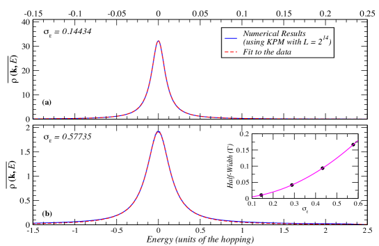
Figure 2: The disorder-averaged spectral function $\rho(k,E)$ of the Anderson model at the band center ($k=\pi/2,$ $E_{k}=0$) for different local variances of the uncorrelated disorder $\sigma_{\varepsilon}^{2}$. The spectral function is well represented by a lorentzian, as expected for low disorder. The black dots in the inset are the corresponding half-widths of the fitted curves; the magenta line is the Born approximation, Eq. 37.

In Figure 2 we show the approximated spectral function for various values of the local variance $\sigma_{\varepsilon}^{2}$, at the band center, i.e. $E_{k}=0$ $(k=\pi/2)$. The data is well fitted by a lorentzian, as expected from perturbation theory. In the inset, we show a comparison between the half-width of the lorentzian, obtained from the fits, and the value calculated from the Born approximation.

$$\hbar\Gamma=\frac{\sigma_{\varepsilon}^{2}}{2}.$$ (37)

This perturbative result seems to give a good account of the data until values $\sigma_{\varepsilon}\lesssim 1$.

The spectral function, at the band center ($E_{k}=0),$ for a gaussian correlated disorder with different values of the parameter $q_{c}$, is shown in Figure 3 for $\sigma_{\varepsilon}=1$. The magenta dashed curves are the corresponding fits. For $q_{c}=\pi$ [Figure 3(a)], the best fit of the numerical data can be found with a lorentzian of width $\Gamma\backsimeq 0.4456$.

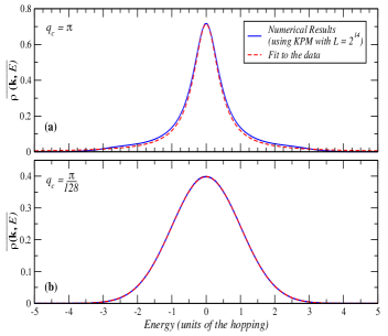
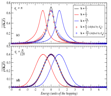
Figure 3: The disorder-averaged spectral function for gaussian correlated disorder with unit variance $\sigma_{\epsilon}^{2}=1,$ for (a) $q_{c}=\pi$, and (b) $q_{c}=\pi/128.$ The spectral functions are reasonably fitted by a lorentzian (upper panel) of half-width $\Gamma\backsimeq 0.4456$, and very well fitted a gaussian (lower panel) of variance $\sigma_{\varepsilon}^{2}=1$. The plots (c) and (d), show the spectral function for different values of $k$ and how it relates to its shape at the band’s center.

When $q_{c}=\pi/128$, the scattering becomes local in momentum space, and the spectral function is seen to be a gaussian [Figure 3(b)]. Its width is just the variance of the site energies, $\sigma_{\varepsilon}^{2},$ as can be seen in Figure 4, where the spectral functions for different values of $\sigma_{\varepsilon}$ are scaled to show that

$$\overline{\rho(k=\pm\frac{\pi}{2},E)}=\sigma_{\varepsilon}^{-1}\mathcal{N}\left(0,1,E/\sigma_{\varepsilon}\right),\quad\textrm{for }\sigma_{\varepsilon}>>\hbar v_{k}q_{c}.$$ (38)

In Eq. 38, $\mathcal{N}(\mu,\sigma,\varepsilon)$ is the normal distribution of mean $\mu$ and variance $\sigma$.

This result calls to mind the classical limit of the spectral function discussed by Trappe et. al. [23]. In that limit, the disordered potential dominates, and the spectral function merely reflects the probability distribution of local potential values. This is, in fact, what is observed here. Since

$$\varepsilon_{m}=2\sum_{q>0}V(q)\cos\left(qm+\phi_{q}\right),$$ (39)

in the thermodynamic limit (i.e. $q_{c}\gg\pi/L$), the energy at each site is a sum of a large number of random independent variables, and by the central limit theorem, it is normally distributed. But what is significant here is that this limit can be obtained even when the disorder strength is small enough to be considered a weak perturbation when compared to the bandwidth. As we will see later this will turn out to be a consequence of the local character of the scattering in momentum space.

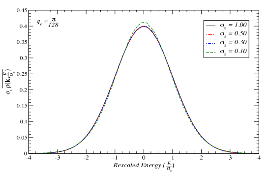
Figure 4: The normalized spectral function for the gaussian correlated disorder of the system of size $L=2^{14}$ with $8192$ Chebyshev coefficients for different values of disorder variance $\sigma_{\varepsilon}$ .

3.2 Power-Law Correlated Disorder

A power-law correlated disorder is characterized by the exponent $\alpha$ that determines how fast the Fourier transform of $\varepsilon_{n}$ decays with the wavenumber $q$,

$$V^{2}(q)\sim\frac{1}{\left|q\right|^{\alpha}}.$$ (40)

As $\alpha$ increases, scattering becomes increasingly dominated by small values of $q$ ($q\ll\pi)$. In Figure 5, we see that a transition for a lorentzian to a gaussian shape (with unit variance) of the spectral function at the band center and for $\sigma_{\varepsilon}=1$, occurs at $\alpha\approx 1.0$. This transition seems to hold for other values of $k$ as well, as can be seen from the left panels of Figure 5. On closer scrutiny, however, a perfect gaussian fit is only possible for $\alpha\to 1^{+}$, in the large $L$ limit, and deviations become increasingly obvious as $\alpha$ increases; the spectral function develops a two peaked structure as a function of energy, as shown in Figure 5(b) in orange.

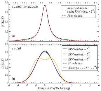
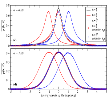
Figure 5: Mean spectral function for two values of the correlation exponent, $\alpha$, and $\sigma_{\varepsilon}=1.$ The numerical plots show a good agreement with the following conclusions: (a) and (c) a lorentzian fit of width $\Gamma\thicksim 0.433$ and a strong dependence of the shape with the value of $k$, for $\alpha<1$; (b) and (d) a gaussian fit of unit variance in the large $L$ limit and a very weak dependence of the shape with the value of $k$ for $\alpha\sim 1^{+}$. In (b) an example of numerical data for $\alpha=2.5$ illustrates the double-peak structure which emerges for higher values of the exponent.

Even though the form of the spectral function is not a gaussian, one still observes (Figure 6) a universal behavior, for different disorder strengths, similar to the one found for gaussian disorder, namely

$$\overline{\rho(k,E)}=\sigma_{\varepsilon}^{-1}\chi_{\alpha}\left(\frac{E}{\sigma_{\varepsilon}}\right)$$ (41)

with the $\chi_{\alpha}(\varepsilon$) depending on $\alpha$, but not on the disorder variance $\sigma_{\varepsilon}$.

As for the gaussian disorder case, we will show that the results of Figs. 5b and 6 reveal the emergence of the classical limit, as a consequence of the local character of scattering in momentum space.

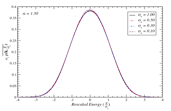
Figure 6: The rescaled mean spectral function for the power-law correlated disorder, in a system of size $L=2^{14}$ for different values of the on-site variance $\sigma_{\varepsilon}$. There were used $8192$ Chebyshev coefficients for the calculation.

3.3 Statistical properties of the spectral function in the thermodynamic limit

Thus far we have discussed the disorder-averaged spectral function. It is not however clear if this quantity represents a typical value for measurable quantity of macroscopic systems. This becomes specially concerning in the case of the power-law disorder model, which is known to have pathological properties in the thermodynamic limit[17]. To investigate this issue, we calculated the standard deviation of $\rho(k,E)$ for increasing number of sites and different values of the exponent $\alpha$. These results are shown for two examples in Figure 7.

From the numerical data, we conclude that for $\alpha<1$ the standard deviation scales as $L^{-\nicefrac{{1}}{{2}}}$, which clearly indicates a self-averaging behavior. On the other hand, for $\alpha>1$ there seems to be a finite standard deviation for $\rho(k,E)$, even in the thermodynamic limit, i.e. $\rho(k,E)$ still fluctuates from sample to sample in the macroscopic limit. This property clearly indicates that $\alpha=1$ is a special value for these models, not only because the shape of $\overline{\rho(k,E)}$ changes, but also because it becomes a non-self-averaging quantity.

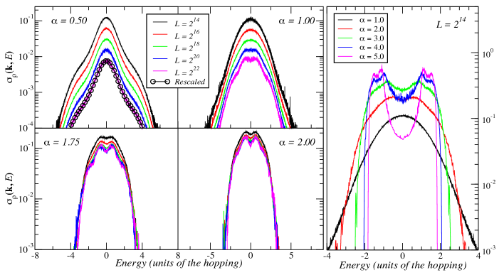
Figure 7: Plots of the standard deviation of the spectral function at $k=\pm\frac{\pi}{2}$, for $\alpha=0.5$ (upper left panel), $\alpha=1.0$ (upper right panel), $\alpha=1.75$ (lower left panel) and $\alpha=2.0$ (lower right panel). For $\alpha=0.5$ the consecutive curves are shown to collapse when rescaled by a factor of $L^{-\nicefrac{{1}}{{2}}}$ (black dots). For $\alpha>1$, the curves coalesce to a non-zero limiting profile and no qualitative change of behavior is seen across $\alpha=2$. In the extreme right panel, we show the decrease of the standard deviation for larger values of $\alpha$ (at a fixed size). All the calculations where done with $\sigma_{\varepsilon}=1$.

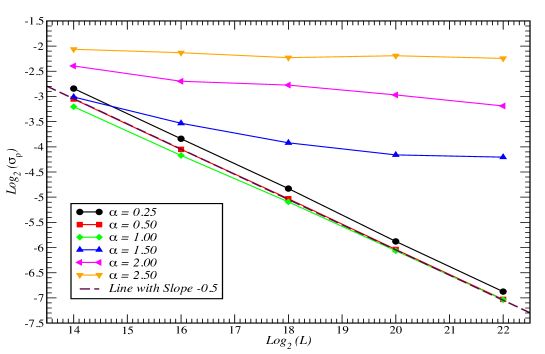
Figure 8: Scaling of the standard deviation of $\rho(k,E)$ for $k=\frac{\pi}{2}$ and $E=0$, as a function of the system’s size. The dashed line stands for the usual $L^{-\nicefrac{{1}}{{2}}}$ scaling.

In Figure 7, we can also see an example of the same calculation done for $\alpha=2$, where no qualitative changes in the scaling behavior of $\sigma_{\rho}$ can be seen. Obviously, for very large values of $\alpha$, these persistent fluctuations start to decrease, since the system is approaching an ordered limit ($\alpha\rightarrow+\infty$). To sum up these results, we present in Figure 8, a plot showing the scaling of $\sigma_{\rho}$ at the central energy, with the increase in the chain size.

4 Analytical Results and Discussion

If the state at $t=0$ is $\left|\psi(0)\right\rangle=\left|k\right\rangle$, the probability amplitude that the state at time $t$ is still the same is $\left\langle k\right|e^{-i\mathcal{H}t/\hbar}\left|k\right\rangle$. Using a complete set of energy eigenstates $\left\{\left|\psi_{\beta}\right\rangle:\text{$\beta=0,\dots,N-1$}\right\}$, we can see that this amplitude is the Fourier transform of the spectral function defined in Eq .32:

$$\left\langle k\right|e^{-i\mathcal{H}t/\hbar}\left|k\right\rangle =\sum_{\beta}e^{-iE_{\beta}t/\hbar}\left|\langle\psi_{\beta}|k\rangle\right|^{2}$$

$$=\int_{-\infty}^{+\infty}dEe^{-iEt/\hbar}\sum_{\beta}\left|\langle\psi_{\beta}|k\rangle\right|^{2}\delta\left(E-E_{\beta}\right)$$

$$=\int_{-\infty}^{+\infty}dEe^{-iEt/\hbar}\rho(k,E).$$ (42)

Expanding both sides in powers of $t$ and averaging over disorder, we get the following expression for the $n^{th}$-moment of the disorder-averaged spectral function $\overline{\rho(k,E)}$:

$$\overline{\left\langle k\right|\mathcal{H}^{n}\left|k\right\rangle}=\int_{-\infty}^{+\infty}dEE^{n}\overline{\rho\left(k,E\right)}.$$ (43)

The Hamiltonian is the one defined in Eq. 1 and can be written as $\mathcal{H}=\mathcal{H}_{0}+\mathcal{V}$ where

$$\mathcal{H}_{0}= \sum_{k}E_{k}\left|k\right\rangle\left\langle k\right|$$ (44a)

$$\mathcal{V}= \sum_{m}\varepsilon_{m}\left|\varphi_{m}\right\rangle\left\langle\varphi_{m}\right|,$$ (44b)

with the band Hamiltonian $\mathcal{H}_{0}$ being diagonal in the Bloch basis, and the disordered potential, $\mathcal{V},$ in the local Wannier basis. In the calculation of $\left\langle k\right|\mathcal{H}^{n}\left|k\right\rangle$, we will assume that $\mathcal{H}_{0}\left|k\right\rangle=E_{k}\left|k\right\rangle=0$. This is strictly true for the states in the center of the band (i.e $k=\pm\pi/2$), for which we calculated numerically the spectral function. However, this assumption implies no loss of generality, since for an arbitrary value $k$, we can add an irrelevant constant to $\mathcal{H}$,

$$\mathcal{H}_{0}\to\mathcal{H}_{0}:=\sum_{k^{\prime}}\left(E_{k^{\prime}}-E_{k}\right)\left|k^{\prime}\right\rangle\left\langle k^{\prime}\right|,$$ (45)

such that $\mathcal{H}_{0}\left|k\right\rangle=0$, remains true. The calculation will show that changing $k$ only shifts the spectral function in energy, by the value of $E_{k}$.

4.1 Gaussian case

As a justification for our numerical results, we managed to calculate the average spectral function for the infinite chain, with a gaussian model of correlated disorder. Generally, our analytical results will be valid in the limits when $2\pi/L\ll q_{c}\ll\pi$ and $q_{c}\ll\sigma_{\varepsilon}/\hbar v_{k}$.

4.1.1 Lowest Order Terms

To illustrate the gist of the argument, we begin by looking at the lowest order moments, using the Eq. 43.

It is obvious that for $n=1$ the result is zero, because $\mathcal{H}_{0}\left|k\right\rangle=0$ and $\overline{\mathcal{V}}=0$. For $n=2,$

$$\overline{\left\langle k\right|\mathcal{H}^{2}\left|k\right\rangle}= \overline{\left\langle k\right|(\mathcal{H}_{0}+\mathcal{V})(\mathcal{H}_{0}+\mathcal{V})\left|k\right\rangle}$$

$$= \overline{\left\langle k\right|\mathcal{V}^{2}\left|k\right\rangle},$$ (46)

and resolving the identity in the Bloch basis,

$$\overline{\left\langle k\right|\mathcal{H}^{2}\left|k\right\rangle}=\sum_{q}\overline{\left\langle k\right|\mathcal{V}\left|k+q\right\rangle\left\langle k+q\right|\mathcal{V}\left|k\right\rangle}.$$ (47)

Recalling Eq. 8,

$$\overline{\left\langle k\right|\mathcal{H}^{2}\left|k\right\rangle}=\sum_{q}V^{2}(q)=\sigma_{\varepsilon}^{2},$$ (48)

By the same arguments, in the third moment only one term survives:

$$\overline{\left\langle k\right|\mathcal{H}^{3}\left|k\right\rangle} =\overline{\left\langle k\right|\mathcal{V}\mathcal{H}_{0}\mathcal{V}\left|k\right\rangle}$$

$$=\sum_{q}V^{2}(q)E_{k+q};$$ (49)

In the thermodynamic limit, the sum over $q$ turns into an integral and if $q_{c}\ll\pi$, we can extend the integration range to $q\in\left]-\infty,\infty\right[$ and expand $E_{k+q}\approx\hbar v_{k}q$. In this case, the integrand is odd in $q$ and the right-hand side of Eq. 49 vanishes upon integration.

Finally, we tackle the $4^{th}$-moment (the last, before presenting the general argument), whose the only non-zero terms are

$$\overline{\left\langle k\right|\mathcal{\mathcal{H}}^{4}\left|k\right\rangle}=\overline{\left\langle k\right|\mathcal{\mathcal{V}}\mathcal{H}_{0}^{2}\mathcal{V}\left|k\right\rangle}+\overline{\left\langle k\right|\mathcal{\mathcal{V}}^{4}\left|k\right\rangle}.$$ (50)

Using the same technique as above, the first term is

$$\sum_{q}V^{2}(q)E_{k+q}^{2}=\sum_{q}V^{2}(q)\left(\hbar v_{k}q\right)^{2},$$ (51)

which is a complete gaussian integral (in the limit $q_{c}\ll\pi$), whose value is

$$\left\langle k\right|\mathcal{\mathcal{V}}\mathcal{H}_{0}^{2}\mathcal{V}\left|k\right\rangle=\sigma_{\varepsilon}^{2}\left(\hbar v_{k}q_{c}\right)^{2}.$$ (52)

On the other hand, the term containing the $4^{th}$ power of $\mathcal{V}$ is

$$\overline{\left\langle k\right|\mathcal{\mathcal{V}}^{4}\left|k\right\rangle} =\sum_{q_{1},q_{2},q_{3}}V(q_{1})V(q_{2})V(q_{3})V(-q_{1}-q_{2}-q_{3})$$

$$\times\overline{e^{i\phi_{q_{1}}}e^{i\phi_{q_{2}}}e^{i\phi_{q_{3}}}e^{i\phi_{-q_{1}-q_{2}-q_{3}}}},$$

The averages of these random phase factors are discussed in the A. In particular, we show that, in the thermodynamic limit ($L\rightarrow\infty$), the expression above reduces to

$$\overline{\left\langle k\right|\mathcal{\mathcal{V}}^{4}\left|k\right\rangle}=3\left[\sum_{q}V^{2}\left(q\right)\right]^{2}=3\sigma_{\varepsilon}^{4}.$$ (53)

Finally, by looking at the Eqs. 52 and 53, we see that, as long as $\sigma_{\varepsilon}^{2}\gg\left(\hbar v_{k}q_{c}\right)^{2}$, we can ignore terms that have insertions of $\mathcal{H}_{0}$. Then, we simply write $\overline{\left\langle k\right|\mathcal{\mathcal{H}}^{4}\left|k\right\rangle}$ as:

$$\overline{\left\langle k\right|\mathcal{\mathcal{H}}^{4}\left|k\right\rangle}\approx\overline{\left\langle k\right|\mathcal{\mathcal{V}}^{4}\left|k\right\rangle}=3\sigma_{\varepsilon}^{4}$$ (54)

4.1.2 General Expression for the Moments of $\rho(k,E)$

Inspired on the results above, we argue that the general form of the terms in Eq. 43 is:

$$\overline{\left\langle k\right|\mathcal{\mathcal{H}}^{2p}\left|k\right\rangle}\approx\overline{\left\langle k\right|\mathcal{\mathcal{V}}^{2p}\left|k\right\rangle},$$ (55)

$$\overline{\left\langle k\right|\mathcal{\mathcal{H}}^{2p+1}\left|k\right\rangle}\approx 0.$$ (56)

Furthermore, in the A we show that the averages $\overline{\left\langle k\right|\mathcal{V}^{2p}\left|k\right\rangle}$ have the following general form

$$\overline{\left\langle k\right|\mathcal{V}^{2p}\left|k\right\rangle}=(2p-1)!!\left(\sigma_{\varepsilon}^{2}\right)^{p}\left[1+\mathcal{O}\left(\frac{1}{L}\right)\right].$$ (57)

Using the Eqs. 55-57, in the thermodynamic limit ($L\rightarrow\infty$), we can rebuild the entire Taylor series for the averaged diagonal propagator, and re-sum it as follows:

$$\overline{\left\langle k\right|e^{-i\mathcal{H}t/\hbar}\left|k\right\rangle} =\sum_{p=0}^{\infty}\frac{1}{(2p)!}\left(\frac{-it}{\hbar}\right)^{2p}\overline{\left\langle k\right|\mathcal{\mathcal{V}}^{2p}\left|k\right\rangle}$$

$$=\sum_{p=0}^{\infty}\frac{(-1)^{p}(2p-1)!!}{(2p)!}\left(\frac{\sigma_{\varepsilon}^{2}t^{2}}{\hbar^{2}}\right)^{p}$$

$$=\sum_{p=0}^{\infty}\frac{1}{2^{p}p!}\left(-\frac{\sigma_{\varepsilon}^{2}t^{2}}{\hbar^{2}}\right)^{p}=e^{-\sigma_{\varepsilon}^{2}t^{2}/2\hbar^{2}}$$

The spectral function is the time-domain Fourier transform of this last expression, yielding

$$\overline{\rho(k=\pm\frac{\pi}{2},E)}=\frac{1}{\sqrt{2\pi\sigma_{\varepsilon}^{2}}}e^{-\frac{E^{2}}{2\sigma_{\varepsilon}^{2}}},$$ (58)

which agrees with the results found in our numerical calculations, using the KPM.

For the sake of completeness, we also state the result for a general value of $k$, which can be obtained from Eq. 58 simply by shifting the energy variable by the corresponding band energy $E_{k}$ of that state, i.e.

$$\overline{\rho(k,E)}=\frac{1}{\sqrt{2\pi\sigma_{\varepsilon}^{2}}}e^{-\frac{\left(E-E_{k}\right)^{2}}{2\sigma_{\varepsilon}^{2}}}.$$ (59)

In conclusion, we found that, if $q_{c}\ll\pi$ and $\left(v_{k}q_{c}\right)^{2}\ll\sigma_{\varepsilon}^{2}$, then the disorder-averaged spectral function, in the thermodynamic limit, will have a gaussian shape. This is true, even if the disorder strength (measured by $\sigma_{\varepsilon}$) is small, as long as this is matched by a decrease of $q_{c}$ and corresponding increase of the correlation length of the potential. For instance, the mean free path, estimated by $\ell=\hbar v_{k}/\sigma_{\varepsilon}$ can still be much larger that the lattice parameter, so long as $\ell<\xi$ , where $\xi$ is the disorder correlation length.

4.1.3 Emergence of the Classical Limit for the Spectral Function

We were able to establish precise conditions in which the classical limit of the spectral function, found by Trappe et. al.[23], appears. The statement of this limit is equivalent to Eq. 55, and reads ($E_{k}=0$)

$$\overline{\left\langle k\right|e^{-i\mathcal{H}t/\hbar}\left|k\right\rangle}=\overline{\left\langle k\right|e^{-i\mathcal{V}t/\hbar}\left|k\right\rangle}.$$ (60)

so that

$$\overline{\rho(k,E)}=\int dte^{iEt/\hbar}\overline{\left\langle k\right|e^{-i\mathcal{V}t/\hbar}\left|k\right\rangle}.$$ (61)

Using the Wannier basis (eigenbasis of $\mathcal{V}$) and its transformation law to the Bloch basis $\langle\varphi_{n}|k\rangle=\exp\left(ikn\right)/\sqrt{L}$, we can rewrite the above equation (with $E_{k}=0$) as

$$\overline{\left\langle k\right|e^{-i\mathcal{V}t/\hbar}\left|k\right\rangle} =\sum_{n,m}\overline{\langle k|\varphi_{n}\rangle\left\langle\varphi_{n}\right|e^{-i\mathcal{V}t/\hbar}\left|\varphi_{m}\right\rangle\langle\varphi_{m}|k\rangle}$$

$$=\frac{1}{L}\sum_{m}\overline{e^{-i\varepsilon_{m}t/\hbar}}=\int dEP(E)e^{-iEt/\hbar},$$ (62)

where $P(E)$ is the probability distribution of a site energy. Comparing the above with Eq. 42, we have

$$\overline{\rho(k,E)}=P(E).$$ (63)

Thus, the averaged spectral function is just the probability distribution of a single site energy. As it is clear for the definition of the disordered potential (Eq. 4), the distribution $P(E)$ must be a gaussian according of the Central Limit Theorem.

4.2 Power-Law Correlated Disorder

4.2.1 Validity of the Classical Limit

In the case of Power-law correlated disorder, the argument leading to the Eq. 55 still holds, as long as $\alpha>1$, but requires a slightly different formulation. To see how this comes about, let us consider Eq. 51 as an example. In this case, we have

$$\sum_{q}V^{2}(q)E_{k+q}^{2} =\frac{2\pi}{L}A^{2}(\alpha)\sum_{q\neq 0}\frac{1}{\left|q\right|^{\alpha}}\left[E_{k+q}\right]^{2}$$

$$=\frac{\sigma_{\varepsilon}^{2}}{2\mathcal{\zeta}(\alpha)}\sum_{p=1}^{L/2}\frac{1}{p^{\alpha}}E_{k+2\pi p/L}^{2}.$$ (64)

As before, if we expand $E_{k+q}$ in powers of $p$, we get terms of the form

$$\left[\frac{1}{n!}\frac{d^{n}E_{k}}{dk^{n}}\right]\frac{\sigma_{\varepsilon}^{2}}{2\mathcal{\zeta}(\alpha)}\left(\frac{2\pi}{L}\right)^{n}\sum_{p=1}^{L/2}\frac{1}{p^{\alpha-n}}$$ (65)

If $\alpha-n>1$ the sum above is convergent and the result vanishes, in the large-$L$ limit, as $L^{-n}.$ On the other hand, if $\alpha-n<1$ the sum diverges, but instead it can be written as an integral over the First Brillouin Zone, as follows

$$\left(\frac{2\pi}{L}\right)^{n}\sum_{p=1}^{L/2}\frac{1}{p^{\alpha-n}} =\left(\frac{2\pi}{L}\right)^{\alpha-1}\int_{\frac{2\pi}{L}}^{\pi}dq\frac{1}{q^{\alpha-n}}$$

$$= \frac{1}{n-\alpha+1}\left[\frac{2^{\alpha-1}\pi^{n}}{L^{\alpha-1}}-\left(\frac{2\pi}{L}\right)^{n}\right].$$ (66)

Both terms in the equation above go to zero in the thermodynamic limit, since $\alpha>1$ and $n\geq 1$. This argument is obviously true for every term in $\left\langle k\right|\mathcal{H}^{n}\left|k\right\rangle$, containing insertions of $\mathcal{H}_{0}$. Hence, in the $L\rightarrow\infty$ limit, the only finite contributions come from the all-$\mathcal{V}$ terms, and we re-obtain the classical result expressed in Eq. 63.

In this limit the spectral function can only depend on the parameters of the disordered potential, namely $\sigma_{\varepsilon}$ and $\alpha$. Since $\alpha$ is dimensionless, there is a single energy scale, $\sigma_{\varepsilon}$, in $\overline{\rho(k,E)}$. The scaling of Eq. 41, illustrated in Figure 6, follows at once. It should be noted, however, that as $\alpha$ gets closer to 1, this scaling is not observed numerically. This is due to finite size effects that we have not accounted for. An example is the very slow convergence of $\sum_{p=1}^{L/2}p^{-\alpha}$ to $\zeta(\alpha)$. For $\alpha=1.1,$ for instance, the truncation error is still of order 10% for $L\sim 10^{10}.$

4.2.2 The Limiting Cases ($\alpha\rightarrow 1$ and $\alpha\rightarrow+\infty$) And The Double-Peaked Shape

Despite the validity of the classical limit for the averaged spectral function, we have shown in the A that it is not clear how to obtain a closed form for the $n^{th}$-moment of $\overline{\rho(k,E)}$ even in this limit. Nevertheless, the limit $\alpha\rightarrow 1^{+}$ revealed itself as very special case, where the exact averaged spectral function is found to be a gaussian,

$$\overline{\rho(k,E)}=\frac{1}{\sqrt{2\pi\sigma_{\varepsilon}^{2}}}e^{-\frac{\left(E-E_{k}\right)^{2}}{2\sigma_{\varepsilon}^{2}}}.$$ (67)

This result is consistent with the numerical results obtained in the last section (see Figure 5).

For $\alpha>1$, however, the higher cumulants of the spectral function cease to be zero, and $\overline{\rho(k,E)}$ drifts away from a gaussian shape. For illustration, we have calculated the $4^{th}$-cumulant of the averaged spectral function, as a function of the exponent $\alpha$ . This has the following definition:

$$m_{4}=\int_{-\infty}^{+\infty}dEE^{4}\overline{\rho\left(k,E\right)}-3\left[\int_{-\infty}^{+\infty}dEE^{2}\overline{\rho\left(k,E\right)}\right]^{2},$$ (68)

and can be directly computed using the expressions obtained in the A, i.e.

$$m_{4}(\alpha)=-3\sigma_{\varepsilon}^{4}\frac{\zeta(2\alpha)}{2\zeta(\alpha)}.$$ (69)

Other than explaining the deviations from the gaussian shape that we found in the numerical plots of $\overline{\rho(k,E)}$, these effects have another striking consequence. According to our earlier remarks, in the classical limit, the averaged spectral function is the same as the probability distribution of the site energies. Since the value of the disordered potential in a single point is described as a sum of a large number of independent random variables (see Eq. 18), the non gaussian shape shows that these do not obey the Central Limit Theorem. To see how this comes about, we start by looking at Eq. 23, where

$$\sigma_{\varepsilon}^{2}\propto\sum_{p=1}^{L/2}\frac{1}{p^{\alpha}}.$$ (70)

When $\alpha>1$, this sum is convergent in the $L\to\infty$ limit, which means that only a number of $\mathcal{O}(1)$ of terms actually contribute to the variance of the local disorder $\varepsilon_{n}$. Furthermore, as $\alpha$ increases, this sum is dominated by less and less terms, meaning that we are never in the conditions of the central limit theorem (which assumes a large number of summed random independent variables).

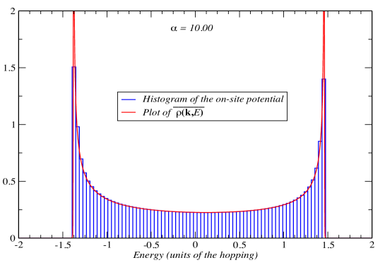
Figure 9: Comparison of the local energy distribution $P(E)$ and the disorder-averaged spectral function $\overline{\rho(k,E)}$, obtained for a system of size $L=2^{17}$ with $8192$ Chebyshev expansion coefficients and a single realization of disorder. The calculation was done for $k=\nicefrac{{\pi}}{{2}}$.

This becomes particularly clear in the extreme case $\alpha\rightarrow+\infty$. In this limit, the local value of the disordered potential is dominated by a single term, $p=1$, and the disorder is a static cosine potential with a wavelength $L$ and a random phase,

$$\varepsilon_{n}\sim\sqrt{2}\sigma_{\varepsilon}^{2}\cos(\frac{2\pi n}{L}+\phi_{2\pi/L}).$$ (71)

The corresponding probability density function can be calculated, yielding the expression:

$$P(E)=\frac{1}{\pi}\frac{1}{\sqrt{2\sigma_{\varepsilon}^{2}-E^{2}}}.$$ (72)

As an illustration, we depict in Figure 9 the KPM calculated the spectral function for $\alpha=10,$ and the normalized histogram of site energies for a single realization of disorder. As $\alpha$ increases above $1$, the spectral function smoothly approaches the limiting form of Eq. 72, by first displaying a two peaked shape as illustrated in Figure 10a.

The expression of Eq. 72 also corresponds to the one we obtain numerically for gaussian disorder case when $q_{c}\ll 2\pi/L$ (see Figure 10b). In either case, of course, a single value $q$ dominates the sum

$$\varepsilon_{n}=2\sum_{q>0}V(q)\cos\left(qn+\phi_{q}\right)$$ (73)

and the two models of disorder cannot be distinguished.

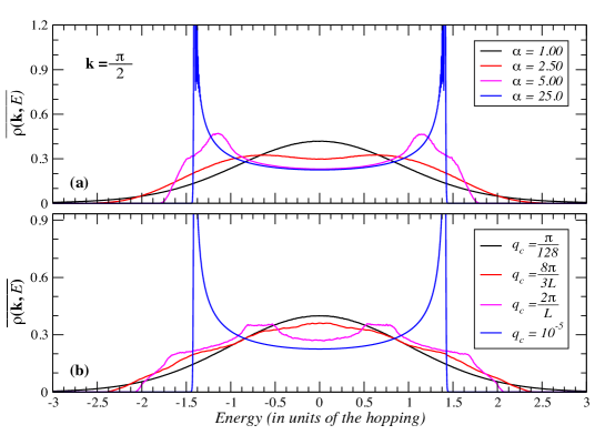
Figure 10: Spectral function $\rho(\mathbf{k},E)$ for the disordered system of size $L=2^{14}$ with $8192$ Chebyshev moments for different values of $\alpha$ (top panel) and $q_{c}$ (lower panel). The limits $\alpha\gg 1$ and $q_{c}\ll 2\pi/L$ are identical: see text .

5 Conclusions

We have studied the spectral function of Bloch states in a tight-binding chain, with two models of correlated disorder: the gaussian model (with a correlation length given by $q_{c}^{-1}$) and the power-law model (with an algebraic decay of correlations characterized by an exponent $\alpha$). For both models, we calculated numerically (with KPM), and analytically, in certain limits, the disorder-averaged single-particle spectral function $\overline{\rho(k,E)}$, at zero temperature. We also evaluated numerically the fluctuations of this quantity from sample to sample, in the power-law model, in order to study its self-averaging character.

The analytical calculations of $\overline{\rho(k,E)}$ were done in the thermodynamic limit, by resuming the short-time expansion of the diagonal propagator in momentum space. For the gaussian case, we found out that, in the regimes when $q_{c}\ll\sigma_{\varepsilon}/\hbar v_{k}$, and the correlation length of the disorder is much larger than the lattice spacing ($q_{c}a\ll 1)$ but much smaller than the system’s size, the spectral function has a gaussian shape, $\rho(k,E)$ with mean $\mu=E_{k}$ and variance $\sigma_{\varepsilon}^{2}$, the variance of the random site energy. This is consistent with the classical limit for the propagator[23] applied to our lattice system.

In the power-law model, where there is no energy scale associated with the space-correlations, we still found that the averaged spectral function is given by its classical limit, but only if the exponent $\alpha$, characterizing the algebraic decay of the power-spectrum, exceeds unity (while the delocalization of the eigenstates[6] occurs only at $\alpha=2$). The mean spectral function is a gaussian in the limit $\alpha\rightarrow 1^{+}$, but develops non-zero higher cumulants for larger values of $\alpha$, reflecting the actual distribution of on-site energies. The spectral density follows a scaling law similar to the one found for the gaussian disorder case. Although we are unable to find an exact functional form for $\overline{\rho(k,E)}$, this scaling law can be understood from the fact that there are no other energy scales in the problem besides $\sigma_{\varepsilon}$ (since $\alpha$ is a dimensionless parameter); hence, $\sigma_{\varepsilon}\overline{\rho(k,E)}$ must be a function of $E/\sigma_{\varepsilon}$. All these results are confirmed by our numerical calculations of $\overline{\rho(k,E)}$.

For the later model, we discovered that the standard deviation of the spectral function, for $\alpha\geq 1$, does not go to zero in the thermodynamic limit. This means that in the non-perturbative regime, the spectral function is not a self-averaging quantity and remains sample dependent in the infinite size system. While this may not come as a surprise in such a pathological model, it also reinforces that $\alpha=1$ is a crossover point for these potentials. More surprisingly, the results on the single-particle spectral function do not seem to give any indication that $\alpha=2$ is a special point for these models, as was argued by Petersen et al[17] in relation to the predicted delocalization transition. Granted that there is no obvious relation between the spectral function and the localization/delocalization of the eigenstates, one could still expect that a qualitative change in the disordered potential might show up at the transition point. Yet, we found no such effect.

In conclusion, we studied the spectral function in a 1D band model with correlated disorder. Through a combination of numerical and analytical work we were able to obtain results in a non-perturbative regime, and show explicitly how the classical limit of the spectral function emerges [23]. In the case of power-law disorder, this happens when the local distribution of site energies is not gaussian, due to inapplicability of the central limit theorem. The localization transition in these models occurs deep in the region where the spectral function is classical, and that raises the question of whether something may be learned on that transition from this knowledge of the spectral function.

6 Acknowledgments

For this work, N. A. Khan was supported by the grants ERASMUS MUNDUS Action 2 Strand 1 Lot 11, EACEA/42/11 Grant Agreement 2013-2538 / 001-001 EM Action 2 Partnership Asia-Europe and research scholarship UID/FIS/04650/2013 of Fundação da Ciência e Tecnologia; J. P. Santos Pires was supported by the MAP-fis PhD grant PD/BD/142774/2018 of Fundação da Ciência e Tecnologia.

The work at Centro de Física do Porto, as a whole, is supported by the grant UID/FIS/04650/2013 of Fundação da Ciência e Tecnologia.

We would also like to thank the referee for its suggestions about the pathological properties of the power-law correlated model, which drove us to extend the paper with the data shown in the Subsection 3.3.

Appendix A Random Phase Averages

In section 4, we needed to calculate terms of the form

$$\overline{\exp\left(i\phi_{q_{1}}\right)\exp\left(i\phi_{q_{2}}\right)\dots\exp\left(i\phi_{-q_{1}-q_{2}-\dots q_{n-1}}\right)}$$ (74)

where $\phi_{q}$ are independent random phases with an uniform distribution in the circle and obeying the constraint $\phi_{q}=-\phi_{q}$. These expressions appear inside sums over momenta, of the form

$$\sum_{q_{1}\neq 0}\dots\sum_{q_{n-1}\neq 0}V(q_{1})\dots V(q_{n-1})V(-q_{1}\dots-q_{n-1})$$

$$\times\overline{\exp\left(i\phi_{q_{1}}\right)\dots\exp\left(i\phi_{-q_{1}-q_{2}-\dots q_{n-1}}\right)}$$ , (75)

where $V(q)=V(-q)$.

Clearly, since these phases are uniformly distributed independent variables (except in the case $q_{2}=\pm q_{1}$), we have

$$\overline{\exp\left(i\phi_{q_{1}}\right)} =0,$$ (76a)

$$\overline{\exp\left(i\phi_{q_{1}}\right)\exp\left(i\phi_{q_{2}}\right)} =\delta_{q_{1}+q_{2},0}.$$ (76b)

Therefore, we can only obtain a non zero result if all the phase factors are paired. This means that $F(q_{1},\dots,q_{n})=\overline{\exp\left(i\phi_{q_{1}}\right)\exp\left(i\phi_{q_{2}}\right)\dots\exp\left(i\phi_{q_{n}}\right)}$ is zero unless $\sum_{i}q_{i}=0$.

General Procedure

To actually calculate the phase averages, we may start with the following illustrative case:

$$F\left(q_{1},q_{2},q_{3},q_{4}\right):=\overline{\exp\left(i\phi_{q_{1}}\right)\exp\left(i\phi_{q_{2}}\right)\exp\left(i\phi_{q_{3}}\right)\exp\left(i\phi_{q_{4}}\right)}$$ (77)

To prevent lengthy notation, we define

$$\delta_{q_{i}+q_{j},0} \to\delta_{ij}$$

$$1-\delta_{q_{i}+q_{j},0} \to\overline{\delta_{ij}}=1-\delta_{ij}$$

such that $\delta_{ij}+\overline{\delta_{ij}}=1$. Note also, that since $V(q)=V(-q)$, the contraction of two momenta is equivalent to a Kronecker delta in the momentum sums.

Hence, we can write

$$F(q_{1},\dots,q_{4}) =\delta_{12}F(q_{3},q_{4})+\overline{\delta_{12}}F(q_{1},\dots,q_{4})$$

$$=\delta_{12}\delta_{34}+\overline{\delta_{12}}F(q_{1},\dots,q_{4}),$$

and repeat the process until we exhaust all possibilities. In this case, we just need to do it once,

$$\overline{\delta_{12}}F(q_{1},\dots,q_{4}) =\overline{\delta_{12}}\left[\delta_{13}\delta_{24}+\overline{\delta_{13}}F(q_{1},\dots,q_{4})\right]$$

$$=\overline{\delta_{12}}\left[\delta_{13}\delta_{24}+\overline{\delta_{13}}\delta_{14}\delta_{23}\right]$$

so

$$F(q_{1},\dots,q_{4})=\delta_{12}\delta_{34}+\overline{\delta_{12}}\delta_{13}\delta_{24}+\overline{\delta_{12}}\overline{\delta_{13}}\delta_{14}\delta_{23}.$$

Finally, if we express everything in terms of Kronecker deltas (using $\overline{\delta_{ij}}:=1-\delta_{ij}$), we get

$$F(q_{1},\dots,q_{4})= \delta_{12}\delta_{34}+\delta_{13}\delta_{24}+\delta_{14}\delta_{23}$$

$$- \delta_{12}\delta_{13}\delta_{24}-\delta_{12}\delta_{14}\delta_{23}-\delta_{13}\delta_{14}\delta_{23}$$

$$+ \delta_{12}\delta_{13}\delta_{14}\delta_{23}.$$ (78)

The left-hand side of the above equation can be divided in three groups of terms:

1. The first three terms correspond to all the pairwise contractions of momenta, which gives a contribution of the form:

   $$3\left(\sum_{q}V^{2}(q)\right)^{2}=3\left(\overline{\epsilon^{2}}\right)^{2}=3\sigma_{\varepsilon}^{4};$$

2. The following three involve double contractions (coincidences of momenta) which imply $V(q_{1})=V(q_{2})=V(q_{3})=V(q_{4})$. This contribution is $-3\sum_{q}V^{4}(q);$

3. The last term gives no contribution, since it implies that $q_{1}=-q_{2}=-q_{3}=-q_{4}$ and $q_{2}=-q_{3}$ . This will always yield a factor of $V(0)=0$.

Consequently, the four momentum sums of Eq. 75 have the value

$$3\left(\sum_{q}V^{2}(q)\right)^{2}-3\sum_{q}V^{4}(q)$$ (79)

This procedure is trivially generalized to any number of phase factors, although the structure becomes rather complicated for higher order terms. Fortunately, we will see that in certain limits, we may ignore the contributions coming from the coincidences of momenta, and only the pairwise contractions will contribute.

Phase Averages in the Gaussian Disorder Case

In the case of the gaussian correlated disorder, the normalization of the Fourier transform implies that $V^{2}(q)\sim\mathcal{O}(1/L)$. The momentum sums give a factor of $\mathcal{O}(L)$, which means that the two terms in Eq. 79 will be of order

$$3\left(\sum_{q}V^{2}(q)\right)^{2} \sim\mathcal{O}(1),$$

$$3\left(\sum_{q}V^{4}(q)\right) \sim\mathcal{O}(L)\times\mathcal{O}(\frac{1}{L^{2}})\sim\mathcal{O}(\frac{1}{L}).$$

This means that the second term is negligible in the thermodynamic limit. This argument can actually be carried through to any order, since any term of the form $\sum_{q}V^{n}(q)$ goes to zero in the limit $L\rightarrow\infty$, which renders all the contributions coming from the coincidence of indices irrelevant in this limit.

Therefore, if we want to calculate a general $F(q_{1},\dots,q_{n})$, we may only consider the sum of all pairwise contractions of momenta. The total number of different contractions is $\left(n-1\right)!!$, and each one contributes with a term $\left(\sum_{q}V^{2}(q)\right)^{\nicefrac{{n}}{{2}}}$to the sum over momenta. Hence, we have

$$\sum_{q_{1}...q_{n-1}}V(q_{1})\;... V(-q_{1}...-q_{n-1})\overline{e^{i\phi_{q_{1}}}...e^{i\phi_{-q_{1}...-q_{n-1}}}}=$$

$$= \left(n-1\right)!!\left(\sum_{q}V^{2}(q)\right)^{\frac{n}{2}}\left[1+\mathcal{O}\left(\frac{1}{L}\right)\right]$$ (80)

Phase Averages in the Power-Law Disorder Case

For the case of Power-Law Correlated Disorder, the Eq. 79 is still valid, but one cannot generally ignore the $V^{4}$ term. Let us consider only the cases where $\alpha>1$, meaning that

$$V(q)=A(\alpha)\left(\frac{2\pi}{L}\right)^{\frac{1}{2}}\frac{1}{\left|q\right|^{\frac{\alpha}{2}}}$$ (81)

with the normalization

$$A(\alpha)=\frac{\sigma_{\varepsilon}}{\sqrt{2\mathcal{\zeta}(\alpha)}}\left(\frac{2\pi}{L}\right)^{\left(\alpha-1\right)/2}.$$ (82)

Like before, we have $\sum_{q\neq 0}V^{2}(q)=\sigma_{\varepsilon}^{2},$ but the calculation of $\sum_{q}V^{4}(q)$ is now, slightly different, i.e.

$$\sum_{q\neq 0}V^{4}(q)= A^{4}\left(\alpha\right)\left(\frac{2\pi}{L}\right)^{2}\sum_{q\neq 0}\frac{1}{\left|q\right|^{2\alpha}}$$

$$= 2A^{4}\left(\alpha\right)\left(\frac{2\pi}{L}\right)^{2\left(1-\alpha\right)}\sum_{p=1}^{L/2}\frac{1}{p^{2\alpha}}$$

In the large $N$ limit, the last sum converges if $\alpha>1/2$ and it gives $\zeta(2\alpha)$. Using Eq. 82, we finally obtain $\sum_{q\neq 0}V^{4}(q)=\frac{\mathcal{\zeta}(2\alpha)}{2\mathcal{\zeta}(\alpha)}\sigma_{\varepsilon}^{4},$ which does not scale with the system size $L$. This interesting result suggests that the argument made for the gaussian case does not work here, and any calculation of the moments of $\rho(k,E)$ must account for the coincidences of momenta. In fact, this is easily seen to be true for any term of the form $\sum_{q}V^{2n}(q)$, yielding the general form

$$\sum_{q}V^{2n}(q)=\frac{\mathcal{\zeta}(n\alpha)}{2^{n}\mathcal{\zeta}(\alpha)^{n}}\sigma_{\varepsilon}^{2n}$$ (83)

Nevertheless, a special case happens when $\alpha\to 1$. In this limit, the denominator of Eq. 83 diverges as $(\alpha-1)^{-n}$ , while the numerator remains finite near $\alpha=1$. This means that, for $\alpha\rightarrow 1$ the corrections due to the coincidence of momenta become negligible, and we have

$$\sum_{q_{1}...q_{n-1}}V(q_{1})\;... V(-q_{1}...-q_{n-1})\overline{e^{i\phi_{q_{1}}}...e^{i\phi_{-q_{1}...-q_{n-1}}}}=$$

$$= \left(n-1\right)!!\left(\sum_{q}V^{2}(q)\right)^{2n}\left[1+\mathcal{O}\left(\alpha-1\right)\right]$$ (84)

References

- [1] E. Abrahams and C. M. Varma. What angle-resolved photoemission experiments tell about the microscopic theory for high-temperature superconductors. Proceedings of The National Academy of Sciences Of The United States Of America, 97(11):5714–5716, May 2000.
- [2] A. A. Abrikosov, L. P. Gorkov, and I. E. Dzyaloshinski. Methods of Quantum Field Theory in Statistical Physics. Dover Publiations Inc, NY, 1975.
- [3] H. Bruus and K. Flensberg. Many-body quantum theory in condensed matter physics: An introduction. Oxford Graduate texts. Oxford University Press, 2004.
- [4] T. P. Cysne, T. G. Rappoport, A. Ferreira, J. M. V. P. Lopes, and N. M. R. Peres. Numerical calculation of the casimir-polder interaction between a graphene sheet with vacancies and an atom. Phys. Rev. B, 94:235405, December 2016.
- [5] A. Damascelli, Z. Hussain, and Z. X. Shen. Angle-resolved photoemission studies of the cuprate superconductors. Rev. Mod. Phys, 75(2):473–541, April 2003.
- [6] F. A. B. F. de Moura and M. L. Lyra. Delocalization in the 1D Anderson model with long-range correlated disorder. Phys. Rev. Lett., 81(17):3735–3738, October 1998.
- [7] D. H. Dunlap, H. L. Wu, and P. W. Phillips. Absence Of Localization In A Random-Dimer Model. Phys. Rev. Lett., 65(1):88–91, July 1990.
- [8] I. E. Dzyaloshinski and A. I. Larkin. Correlation-Functions For A One-Dimensional Fermi System With Long-Range Interaction (Tomonaga Model). Zhurnal Eksperimentalnoi I Teoreticheskoi Fiziki, 65(1):411–426, 1973.
- [9] F. M. Izrailev, A. A. Krokhin, and N. M. Makarov. Anomalous localization in low-dimensional systems with correlated disorder. Phys. Rep. - Rev. Sect. of Phys. Lett., 512(3):125–254, March 2012.
- [10] F. Jendrzejewski, A. Bernard, K. Mueller, P. Cheinet, V. Josse, M. Piraud, L. Pezze, L. Sanchez-Palencia, A. Aspect, and P. Bouyer. Three-dimensional localization of ultracold atoms in an optical disordered potential. Nature Physics, 8(5):398–403, May 2012.
- [11] R Johnston and B Kramer. Localization In One-Dimensional Correlated Random Potentials. Z. Physik B - Condensed Matter, 63(3):273–281, 1986.
- [12] C. Kim, A. Y. Matsuura, Z. X. Shen, N. Motoyama, H. Eisaki, S. Uchida, T. Tohyama, and S. Maekawa. Observation of spin-charge separation in one-dimensional SrCuO2. Phys. Rev. Lett., 77(19):4054–4057, November 1996.
- [13] S. S. Kondov, W. R. McGehee, J. J. Zirbel, and B. DeMarco. Three-Dimensional Anderson Localization of Ultracold Matter. Science, 334(6052):66–68, October 2011.
- [14] L. Lin, Y. Saad, and C. Yang. Approximating spectral densities of large matrices. SIAM Review, 58(1):34–65, 2016.
- [15] P. Lugan, A. Aspect, L. Sanchez-Palencia, D. Delande, B. Gremaud, C. A. Mueller, and C. Miniatura. One-dimensional Anderson localization in certain correlated random potentials. Phys. Rev. A, 80(2), August 2009.
- [16] C. A. Muller and D. Delande. Disorder and interference: localization phenomena: Ultracold Gases and Quantum Information. XCI Les Houches Summer School Session (Ed. by C. Miniatura et al) - Oxford University Press, 2010.
- [17] G. M. Petersen and N. Sandler. Anticorrelations from power-law spectral disorder and conditions for an Anderson transition. Phys. Rev. B, 87(19), May 2013.
- [18] H. Röder, R. N. Silver, D. A. Drabold, and J. J. Dong. Kernel polynomial method for a nonorthogonal electronic-structure calculation of amorphous diamond. Phys. Rev. B, 55:15382–15385, June 1997.
- [19] G. Semeghini, M. Landini, P. Castilho, S. Roy, G. Spagnolli, A. Trenkwalder, M. Fattori, M. Inguscio, and G. Modugno. Measurement of the mobility edge for 3D Anderson localization. Nature Physics, 11(7):554–559, July 2015.
- [20] R. N. Silver, H. Röder, A. F. Voter, and J. D. Kress. Kernel polynomial approximations for densities of states and spectral functions. J. Comput. Phys., 124(1):115 – 130, 1996.
- [21] P. Soven. Coherent-Potential Model Of Substitutional Disordered Alloys. Phys. Rev., 156(3):809–&, 1967.
- [22] H. M. Srivastava, M. L. Glasser, and V. S. Adamchik. Series Associated with the Zeta and Related Functions. Oxford Graduate texts. Kluwer Academic Publishers, Dordrecht, Boston, and London, 2001.
- [23] M. I. Trappe, D. Delande, and C. A. Mueller. Semiclassical spectral function for matter waves in random potentials. Jour. Phys. A - Mathematical And Theoretical, 48(24, SI), June 2015.
- [24] B. Velicky, S. Kirkpatrick, and H. Ehrenreich. Single-Site Approximations In Electronic Theory Of Simple Binary Alloys. Phys. Rev., 175(3):747+, 1968.
- [25] V. V. Volchkov, M. Pasek, V. Denechaud, M. Mukhtar, A. Aspect, D. Delande, and V. Josse. Measurement of spectral functions of ultracold atoms in disordered potentials. Phys. Rev. Lett., 120:060404, February 2018.
- [26] A. Weiße, G. Wellein, A. Alvermann, and H. Fehske. The kernel polynomial method. Rev. Mod. Phys., 78:275–306, March 2006.
- [27] R. Zimmermann and C. Schindler. Coherent potential approximation for spatially correlated disorder. Phys. Rev. B, 80(14):144202, October 2009.