Nonparametric Topic Modeling with Neural Inference

Abstract

This work focuses on combining nonparametric topic models with Auto-Encoding Variational Bayes (AEVB). Specifically, we first propose iTM-VAE, where the topics are treated as trainable parameters and the document-specific topic proportions are obtained by a stick-breaking construction. The inference of iTM-VAE is modeled by neural networks such that it can be computed in a simple feed-forward manner. We also describe how to introduce a hyper-prior into iTM-VAE so as to model the uncertainty of the prior parameter. Actually, the hyper-prior technique is quite general and we show that it can be applied to other AEVB based models to alleviate the collapse-to-prior problem elegantly. Moreover, we also propose HiTM-VAE, where the document-specific topic distributions are generated in a hierarchical manner. HiTM-VAE is even more flexible and can generate topic distributions with better variability. Experimental results on 20News and Reuters RCV1-V2 datasets show that the proposed models outperform the state-of-the-art baselines significantly. The advantages of the hyper-prior technique and the hierarchical model construction are also confirmed by experiments.

1 Introduction

Probabilistic topic models focus on discovering the abstract “topics” that occur in a collection of documents, and represent a document as a weighted mixture of the discovered topics. Classical topic models [4] have achieved success in a range of applications [40, 4, 32, 34]. A major challenge of topic models is that the inference of the distribution over topics does not have a closed-form solution and must be approximated, using either MCMC sampling or variational inference. When some small changes are made on the model, we need to re-derive the inference algorithm. In contrast, black-box inference methods [31, 26, 18, 33] require only limited model-specific analysis and can be flexibly applied to new models.

Among all the black-box inference methods, Auto-Encoding Variational Bayes (AEVB) [18, 33] is a promising one for topic models. AEVB contains an inference network that can map a document directly to a variational posterior without the need for further local variational updates on test data, and the Stochastic Gradient Variational Bayes (SGVB) estimator allows efficient approximate inference for a broad class of posteriors, which makes topic models more flexible. Hence, an increasing number of models are proposed recently to combine topic models with AEVB, such as [24, 37, 7, 25].

Although these AEVB based topic models achieve promising performance, the number of topics, which is important to the performance of these models, has to be specified manually with model selection methods. Nonparametric models, however, have the ability of adapting the topic number to data. For example, Teh et al. [38] proposed Hierarchical Dirichlet Process (HDP), which models each document with a Dirichlet Process (DP) and all DPs for the documents in a corpus share a base distribution that is itself sampled from a DP. HDP has potentially an infinite number of topics and allows the number to grow as more documents are observed. It is appealing that the nonparametric topic models can also be equipped with AEVB techniques to enjoy the benefit brought by neural black-box inference. We make progress on this problem by proposing an infinite Topic Model with Variational Auto-Encoders (iTM-VAE), which is a nonparametric topic model with AEVB.

For nonparametric topic models with stick breaking prior [35], the concentration parameter $\alpha$ plays an important role in deciding the growth of topic numbers. The larger the $\alpha$ is, the more topics the model tends to discover. Hence, people can place a hyper-prior [2] over $\alpha$ such that the model can adapt it to data [9, 38, 5]. Moreover, the AEVB framework suffers from the problem that the latent representation tends to collapse to the prior [6, 36, 8], which means, the prior parameter $\alpha$ will control the number of discovered topics tightly in our case, especially when the decoder is strong. Common heuristic tricks to alleviate this issue are 1) KL-annealing [36] and 2) decoder regularizing [6]. Introducing a hyper-prior into the AEVB framework is nontrivial and not well-done in the community. In this paper, we show that introducing a hyper-prior can increase the adaptive capability of the model, and also alleviate the collapse-to-prior issue in the training process.

To further increase the flexibility of iTM-VAE, we propose HiTM-VAE, which model the document-specific topic distribution in a hierarchical manner. This hierarchical construction can help to generate topic distributions with better variability, which is more suitable in handling heterogeneous documents.

The main contributions of the paper are:

• We propose iTM-VAE and iTM-VAE-Prod, which are two novel nonparametric topic models equipped with AEVB, and outperform the state-of-the-art models on the benchmarks.

• We propose iTM-VAE-HP, in which a hyper-prior helps the model to adapt the prior parameter to data. We also show that this technique can help other AEVB-based models to alleviate the collapse-to-prior problem elegantly.

• We propose HiTM-VAE, which is a hierarchical extension of iTM-VAE. This construction and its corresponding AEVB-based inference method can help the model to learn more topics and produce topic proportions with higher variability and sparsity.

2 Related Work

Topic models have been studied extensively in a variety of applications such as document modeling, information retrieval, computer vision and bioinformatics [3, 4, 40, 30, 32, 34]. Recently, with the impressive success of deep learning, the proposed neural topic models [11, 20, 26] achieve encouraging performance in document modeling tasks. Although these models achieve competitive performance, they do not explicitly model the generative story of documents, hence are less explainable.

Several recent work proposed to model the generative procedure explicitly, and the inference of the topic distributions in these models is computed by deep neural networks, which makes these models explainable, powerful and easily extendable. For example, Srivastava and Sutton [37] proposed AVITM, which embeds the original LDA [4] formulation with AEVB. By utilizing Laplacian approximation for the Dirichlet distribution, AVITM can be optimized by the SGVB estimator efficiently. AVITM achieves the state-of-the-art performance on the topic coherence metric [22], which indicates the topics learned match closely to human judgment.

Nonparametric topic models [38, 15, 1, 23], potentially have infinite topic capacity and can adapt the topic number to data. Nalisnick and Smyth [28] proposed Stick-Breaking VAE (SB-VAE), which is a Bayesian nonparametric version of traditional VAE with a stochastic dimensionality. iTM-VAE differs with SB-VAE in 3 aspects: 1) iTM-VAE is a kind of topic model for discrete text data. 2) A hyper-prior is introduced into the AEVB framwork to increase the adaptive capability. 3) A hierarchical extension of iTM-VAE is proposed to further increase the flexibility. Miao et al. [25] proposed GSM, GSB, RSB and RSB-TF to model documents. RSB-TF uses a heuristic indicator to guide the growth of the topic numbers, and can adapt the topic number to data.

3 The iTM-VAE Model

In this section, we describe the generative and inference procedure of iTM-VAE and iTM-VAE-Prod in Section 3.1 and Section 3.2. Then, Section 3.3 describes the hyper-prior extension iTM-VAE-HP.

3.1 The Generative Procedure of iTM-VAE

Suppose the atom weights $\bm{\pi}=\{\pi_{k}\}_{k=1}^{\infty}$ are drawn from a GEM distribution [27], i.e. $\bm{\pi}\sim\text{GEM}(\alpha)$, where the GEM distribution is defined as:

$$\nu_{k}\sim\text{Beta}(1,\alpha)\qquad\pi_{k}=\nu_{k}\prod_{l=1}^{k-1}(1-\nu_{l})=\nu_{k}(1-\sum_{l=1}^{k-1}\pi_{l}).$$ (1)

Let $\bm{\theta}_{k}=\sigma(\bm{\phi}_{k})$ denotes the $k$th topic, which is a multinomial distribution over vocabulary, $\bm{\phi}_{k}\in\mathbb{R}^{V}$ is the parameter of $\bm{\theta}_{k}$, $\sigma(\cdot)$ is the softmax function and $V$ is the vocabulary size. In iTM-VAE, there are unlimited number of topics and we denote $\Theta=\{\bm{\theta}_{k}\}_{k=1}^{\infty}$ and $\Phi=\{\bm{\phi}_{k}\}_{k=1}^{\infty}$ as the collections of these countably infinite topics and the corresponding parameters. The generation of a document $\bm{x}^{(j)}=\bm{w}^{(j)}_{1:N^{(j)}}$ by iTM-VAE can then be mathematically described as:

• Get the document-specific $G^{(j)}(\bm{\theta};\bm{\pi}^{(j)},\Theta)=\sum_{k=1}^{\infty}\pi_{k}^{(j)}\delta_{\bm{\theta}_{k}}(\bm{\theta})$, where $\bm{\pi}^{(j)}\sim\text{GEM}(\alpha)$

• For each word $w_{n}$ in $\bm{x}^{(j)}$: 1) draw a topic $\hat{\bm{\theta}}_{n}\sim G^{(j)}(\bm{\theta};\bm{\pi}^{(j)},\Theta)$;  2) $w_{n}\sim\text{Cat}(\hat{\bm{\theta}}_{n})$

where $\alpha$ is the concentration parameter, $\text{Cat}(\hat{\bm{\theta}}_{i})$ is a categorical distribution parameterized by $\hat{\bm{\theta}}_{i}$, and $\delta_{\bm{\theta}_{k}}(\bm{\theta})$ is a discrete dirac function, which equals to $1$ when $\bm{\theta}=\bm{\theta}_{k}$ and $0$ otherwise. In the following, we remove the superscript of $j$ for simplicity.

Thus, the joint probability of ${\bf w}_{1:N}=\{w_{n}\}_{n=1}^{N}$, $\hat{\bm{\theta}}_{1:N}=\{\hat{\bm{\theta}_{n}}\}_{n=1}^{N}$ and $\bm{\pi}$ can be written as:

$$p({\bf w}_{1:N},\bm{\pi},\hat{\bm{\theta}}_{1:N}|\alpha,\Theta)=p(\bm{\pi}|\alpha)\prod_{n=1}^{N}p(w_{n}|\hat{\bm{\theta}}_{n})p(\hat{\bm{\theta}}_{n}|\bm{\pi},\Theta)$$ (2)

where $p(\bm{\pi}|\alpha)=\text{GEM}(\alpha)$, $p(\bm{\theta}|\bm{\pi},\Theta)=G(\bm{\theta};\bm{\pi},\Theta)$ and $p(w|\bm{\theta})=\text{Cat}(\bm{\theta})$.

Similar to [37], we collapse the variable $\hat{\bm{\theta}}_{1:N}$ and rewrite Equation 2 as:

$$p({\bf w}_{1:N},\bm{\pi}|\alpha,\Theta)=p(\bm{\pi}|\alpha)\prod_{n=1}^{N}p(w_{n}|\bm{\pi},\Theta)$$ (3)

where $p(w_{n}|\bm{\pi},\Theta)=\text{Cat}(\bar{\bm{\theta}})$ and $\bar{\bm{\theta}}=\sum_{k=1}^{\infty}\pi_{k}\bm{\theta}_{k}$.

In Equation 3, $\bar{\bm{\theta}}$ is a mixture of multinomials. This formulation cannot make any predictions that are sharper than the distributions being mixed [11], which may result in some topics that are of poor quality. Replacing the mixture of multinomials with a weighted product of experts is one method to make sharper predictions [10, 37]. Hence, a products-of-experts version of iTM-VAE (i.e. iTM-VAE-Prod) can be obtained by simply computing $\hat{\bm{\theta}}$ for each document as $\hat{\bm{\theta}}=\sigma(\sum_{k=1}^{\infty}\pi_{k}\bm{\phi}_{k})$.

3.2 The Inference Procedure of iTM-VAE

In this section, we describe the inference procedure of iTM-VAE, i.e. how to draw ${\bm{\pi}}$ given a document ${\bf w}_{1:N}$. To elaborate, suppose $\bm{\nu}=[\nu_{1},\nu_{2},\ldots,\nu_{K-1}]$ is a $K-1$ dimensional vector, where ${\nu_{k}}$ is a random variable sampled from a Kumaraswamy distribution $\kappa(\nu;a_{k},b_{k})$ parameterized by $a_{k}$ and $b_{k}$ [19, 28], iTM-VAE models the joint distribution $q_{\psi}(\bm{\nu}|{\bf w}_{1:N})$ as:

$$[a_{1},\ldots,a_{K-1};b_{1},\ldots,b_{K-1}] = g({\bf w}_{1:N};\psi)$$ (4)

$$q_{\psi}(\bm{\nu}|{\bf w}_{1:N}) = \prod_{k=1}^{K-1}\kappa(\nu_{k};a_{k},b_{k})$$ (5)

where $g({\bf w}_{1:N};\psi)$ is a neural network with parameters $\psi$. Then, ${\bm{\pi}}=\{\pi_{k}\}_{k=1}^{K}$ can be drawn by:

$$\bm{\nu} \sim q_{\psi}(\bm{\nu}|{\bf w}_{1:N})$$ (6)

$${\bm{\pi}} = ({\pi}_{1},{\pi}_{2},\ldots,{\pi}_{K-1},{\pi}_{K})=(\nu_{1},\nu_{2}(1-\nu_{1}),\ldots,\nu_{k-1}\prod_{n=1}^{K-2}(1-\nu_{n}),\prod_{n=1}^{K-1}(1-\nu_{n}))$$ (7)

In the above procedure, we truncate the infinite sequence of mixture weights $\bm{\pi}=\{\pi_{k}\}_{k=1}^{\infty}$ by $K$ elements, and $\nu_{K}$ is always set to $1$ to ensure $\sum_{k=1}^{K}{\pi}_{k}=1$. Notably, as is discussed in [5], the truncation of variational posterior does not indicate that we are using a finite dimensional prior, since we never truncate the GEM prior. Hence, iTM-VAE still has the ability to model the uncertainty of the number of topics and adapt it to data [28].

iTM-VAE can be optimized by maximizing the Evidence Lower Bound (ELBO):

$$\mathcal{L}({\bf w}_{1:N}|\Phi,\psi)=\mathbb{E}_{q_{\psi}(\bm{\nu}|{\bf w}_{1:N})}\left[\log p({\bf w}_{1:N}|\bm{\pi},\Phi)\right]-\text{KL}\left(q_{\psi}(\bm{\nu}|{\bf w}_{1:N})||p({\bm{\nu}|\alpha})\right)$$ (8)

where $p({\bm{\nu}|\alpha})$ is the product of $K-1$ $\text{Beta}(1,\alpha)$ probabilistic density functions. The details of the optimization can be found in Appendix 1.3.

3.3 Modeling the Uncertainty of Prior Parameter

In the generative procedure, the concentration parameter $\alpha$ of $\text{GEM}(\alpha)$ can have significant impact on the growth of number of topics. The larger the $\alpha$ is, the more “breaks" it will create, and consequently, more topics will be used. Hence, it is generally reasonable to consider placing a hyper-prior on $\alpha$ to model its uncertainty.[9, 5, 38]. For example, Escobar and West [9] placed a Gamma hyper-prior on $\alpha$ for the urn-based samplers and implemented the corresponding Gibbs updates with auxiliary variable methods. Blei et al. [5] also placed a Gamma prior on $\alpha$ and derived a closed-form update for the variational parameters. Different with previous work, we introduce the hyper-prior into the AEVB framework and propose to optimize the model by stochastic gradient decent (SGD) methods.

Concretely, since the Gamma distribution is conjugate to $\text{Beta}(1,\alpha)$, we place a $\text{Gamma}(s_{1},s_{2})$ prior on $\alpha$. Then the ELBO of iTM-VAE-HP can be written as:

$$\mathcal{L}({\bf w}_{1:N}|\Phi,\psi) = \mathbb{E}_{q_{\psi}(\bm{\nu}|{\bf w}_{1:N})}\left[\log p({\bf w}_{1:N}|\bm{\pi},\Phi)\right]+\mathbb{E}_{q_{\psi}(\bm{\nu}|{\bf w}_{1:N})q(\alpha|\gamma_{1},\gamma_{2})}[\log p(\bm{\nu}|\alpha)]$$ (9)

$$-\mathbb{E}_{q_{\psi}(\bm{\nu}|{\bf w}_{1:N})}[\log q_{\psi}(\bm{\nu}|{\bf w}_{1:N})]-\text{KL}(q(\alpha|\gamma_{1},\gamma_{2})||p(\alpha|s_{1},s_{2}))$$

where $p(\alpha|s_{1},s_{2})=\text{Gamma}(s_{1},s_{2})$, $p(v_{k}|\alpha)=\text{Beta}(1,\alpha)$, $q(\alpha|\gamma_{1},\gamma_{2})$ is the corpus-level variational posterior for $\alpha$. The derivation for Equation 9 can be found in Appendix 1.4. In our experiments, we find iTM-VAE-Prod always performs better than iTM-VAE, therefore we only report the performance of iTM-VAE-Prod with hyper-prior, and refer this variant as iTM-VAE-HP. Actually, as discussed in Section 1, the hyper-prior technique can also be applied to other AEVB based models to alleviate the collapse-to-prior problem. In Appendix 1.2, we show that by introducing a hyper-prior to SB-VAE, more latent units can be activated and the model achieves better performance.

4 Hierarchical iTM-VAE

In this section, we describe the generative and inference procedures of HiTM-VAE in Section 4.1 and Section 4.2. The relationship between iTM-VAE and HiTM-VAE is discussed in Section 4.3

4.1 The Generative Procedure of HiTM-VAE

The generation of a document by HiTM-VAE is described as follows:

• Get the corpus-level base distribution $G^{(0)}$: $\bm{\beta}\sim\mbox{GEM}(\gamma);G^{(0)}(\bm{\theta};\bm{\beta},\Theta)=\sum_{i=1}^{\infty}\beta_{i}\delta_{\bm{\theta}_{i}}(\bm{\theta})$

• For each document $\bm{x}^{(j)}=\bm{w}^{(j)}_{1:N^{(j)}}$ in the corpus:

  • Draw the document-level stick breaking weights $\bm{\pi}^{(j)}\sim\mbox{GEM}(\alpha)$

  • Draw document-level atoms $\bm{\zeta}_{k}^{(j)}\sim G_{0}$, $k=1,\cdots,\infty$; Then we get a document-specific distribution $G^{(j)}(\bm{\theta};\bm{\pi}^{(j)},\{\bm{\zeta}_{k}^{(j)}\}_{k=1}^{\infty},\Theta)=\sum_{k=1}^{\infty}\pi_{k}^{(j)}\delta_{\bm{\zeta}_{k}^{(j)}}(\bm{\theta})$

  • For each word $w_{n}$ in the document: 1) draw a topic $\hat{\bm{\theta}}_{n}\sim G^{(j)}$; 2) $w_{n}\sim\mbox{Cat}(\hat{\bm{\theta}}_{n})$

To sample the document-level atoms $\bm{\zeta}^{(j)}=\{\bm{\zeta}_{k}^{(j)}\}_{k=1}^{\infty}$, a series of indicator variables ${\mathbb{c}^{(j)}}=\{c_{k}^{(j)}\}_{k=1}^{\infty}$ are drawn i.i.d: $c_{k}^{(j)}\sim\mbox{Cat}(\bm{\beta})$. Then, the document-level atoms are $\bm{\zeta}_{k}^{(j)}=\bm{\theta}_{c_{k}^{(j)}}$.

Let $D$ and $N^{(j)}$ denote the size of the dataset and the number of word in each document $\bm{x}^{(j)}$, respectively. After collapse the per-word assignment random variables $\{\{\hat{\bm{\theta}}_{n}^{(j)}\}_{n=1}^{N^{(j)}}\}_{j=1}^{D}$, the joint probability of the corpus-level atom weights $\bm{\beta}$, documents $\mathcal{X}=\{\bm{x}^{(j)}\}_{j=1}^{D}$, the stick breaking weights $\Pi=\{\bm{\pi}^{(j)}\}_{j=1}^{D}$ and the indicator variables $\mathcal{C}=\{\bm{c}^{(j)}\}_{j=1}^{D}$ can be written as:

$$p(\bm{\beta},\mathcal{X},\Pi,\mathcal{C}|\gamma,\alpha,\Theta)=p(\bm{\beta}|\gamma)\prod_{j=1}^{D}p(\bm{\pi}^{(j)}|\alpha)p(\bm{c}^{(j)}|\bm{\beta})p(\bm{x}^{(j)}|\bm{\pi}^{(j)},\bm{c}^{(j)},\Theta)$$ (10)

where $p(\bm{\beta}|\gamma)=\text{GEM}(\gamma)$, $p(\bm{\pi}^{(j)}|\alpha)=\text{GEM}(\alpha)$, $p(\bm{c}^{(j)}|\bm{\beta})=\text{Cat}(\bm{\beta})$, $p(x^{(j)}|\bm{\pi}^{(j)},\bm{c}^{(j)},\Theta)=\prod_{n=1}^{N^{(j)}}p(w_{n}^{(j)}|\bm{\pi}^{(j)},\bm{c}^{(j)},\Theta)=\prod_{n=1}^{N^{(j)}}\text{Cat}(w_{n}^{(j)}|\bar{\bm{\theta}}^{(j)})=\prod_{l=1}^{N^{(j)}}\text{Cat}(w_{n}^{(j)}|\sum_{k=1}^{\infty}\pi_{k}^{(j)}\bm{\theta}_{c_{k}^{(j)}})$.

4.2 The Inference Procedure of HiTM-VAE

Setting the truncation level of the corpus-level and document-level GEM to $T$ and $K$, HiTM-VAE models the per-document posterior $q(\bm{\nu},{\mathbb{c}}|{\bf w}_{1:N})$ for every document ${\bf w}_{1:N}$ as:

$$[a_{1},\ldots,a_{K-1};b_{1},\ldots,b_{K-1};\bm{\varphi}_{1},\ldots,\bm{\varphi}_{K}] = g({\bf w}_{1:N};\psi)$$ (11)

$$q(\bm{\nu},{\mathbb{c}}|{\bf w}_{1:N}) = q_{\psi}(\bm{\nu}|{\bf w}_{1:N})q_{\psi}(\bm{c}|{\bf w}_{1:N})$$ (12)

$$q_{\psi}(\bm{\nu}|{\bf w}_{1:N})=\prod_{k=1}^{K-1}\kappa(\nu_{k};a_{k},b_{k});\quad q_{\psi}(\bm{c}|{\bf w}_{1:N}) = \prod_{k=1}^{K}\mbox{Cat}(c_{k};\bm{\varphi}_{k})$$ (13)

where $g({\bf w}_{1:N};\psi)$ is a neural network with parameters $\psi$, and $\bm{\varphi}_{k}=\{\varphi_{ki}\}_{i=1}^{T}$ are the multinomial variational parameters for each document-level indicator variable $c_{k}$. Then, ${\bm{\pi}}=\{\pi_{k}\}_{k=1}^{K}$ can be constructed by the stick breaking process using $\bm{\nu}$.

As we shown in Section 4.1, the generation of the corpus-level atom weights $\bm{\beta}$ is as follows:

$$\beta^{\prime}_{i}\sim\text{Beta}(1,\gamma);\quad\beta_{i}=\beta^{\prime}_{i}\prod_{l=1}^{i-1}(1-\beta^{\prime}_{l})$$ (14)

The corpus-level variational posterior for $\bm{\beta^{\prime}}$ with truncation level $T$ is $q(\bm{\beta^{\prime}})=\prod_{i=1}^{T-1}\text{Beta}(\beta^{\prime}_{i}|u_{i},v_{i})$, where $\{u_{i},v_{i}\}_{i=1}^{T-1}$ are the corpus-level variational parameters.

The ELBO of the training dataset can be written as:

$$\mathcal{L}(\mathcal{D}|\Phi,\psi) = E_{q(\bm{\beta^{\prime}})}[\log\frac{P(\bm{\beta^{\prime}}|\gamma)}{q(\bm{\beta^{\prime}}|\bm{u},\bm{v})}]+\sum_{j=1}^{D}\{E_{q(\bm{\nu}^{(j)})}[\log\frac{P(\bm{\nu}^{(j)}|\alpha)}{q(\bm{\nu}^{(j)})}]+$$

$$\sum_{k=1}^{K}E_{q(\bm{\beta^{\prime}})q(c_{k}^{(j)}|\bm{\varphi}_{k}^{(j)})}[\log\frac{P(c_{k}^{(j)}|\bm{\beta})}{q(c_{k}^{(j)}|\bm{\varphi}_{k}^{(j)})}]+E_{q(\bm{\nu}^{(j)})q(\bm{c}^{(j)})}[P(x^{(j)}|\bm{\nu}^{(j)},\bm{c}^{(j)},\Phi)]\}$$

where $\bm{\beta}=\{\beta_{i}\}_{i=1}^{T}$, $\bm{\nu}^{(j)}=\{\nu_{k}^{(j)}\}_{k=1}^{K-1}$, $\bm{c}^{(j)}=\{c_{k}^{(j)}\}_{k=1}^{K}$, $\bm{\varphi}_{k}^{(j)}=\{\varphi_{ki}^{(j)}\}_{i=1}^{T}$. The details of the derivation of the ELBO can be found in Appendix 1.5.

Gumbel-Softmax estimator [14] is used for backpropagating through the categorical random variables $\bm{c}$. Instead of joint training with the NN parameters, mean-field updates are used to learn the corpus-level variational parameters $\{u_{i},v_{i}\}_{i=1}^{T-1}$:

$$u_{i}=1+\sum_{j=1}^{D}\sum_{k=1}^{K}\varphi_{ki}^{(j)};\quad v_{i}=\gamma+\sum_{j=1}^{D}\sum_{k=1}^{K}\sum_{l=i+1}^{T}\varphi_{kl}^{(j)}$$ (16)

4.3 Discussion

In iTM-VAE, we get the document-specific topic distribution $G^{(j)}$ by sampling the atom weights from a GEM. Instead of being drawn from a continuous base distribution, the atoms are modeled as trainable parameters as in [4, 37, 25]. Thus, the atoms are shared by all documents naturally without the need to use a hierarchical construction like HDP [38]. The hierarchical extension, HiTM-VAE, which models $G^{(j)}$ in a hierarchical manner, is more flexible and can generate topic distributions with better variability. A detailed comparison is illustrated in Section 5.3.

5 Experiments

In this section, we evaluate the performance of iTM-VAE and its variants on two public benchmarks: 20News and RCV1-V2, and demonstrate the advantage brought by the variants of iTM-VAE. To make a fair comparison, we use exactly the same data and vocabulary as [37].

The configuration of the experiments is as follows. We use a two-layer fully-connected neural network for $g({\bf w}_{1:N};\psi)$ of Equation 11, and the number of hidden units is set to $256$ and $512$ for 20News and RCV1-V2, respectively. The truncation level $K$ in Equation 7 is set to $200$ so that the maximum topic numbers will never exceed the ones used by baselines. The concentration parameter $\alpha$ for GEM distribution is cross-validated on validation set from $[10,20,30,50]$ for iTM-VAE and iTM-VAE-Prod. Batch-Renormalization [13] is used to stabilize the training procedure. Adam [16] is used to optimize the model and the learning rate is set to $0.01$. The code of iTM-VAE and its variants is available at http://anonymous.

5.1 Perplexity and Topic Coherence

Perplexity is widely used by topic models to measure the goodness-to-fit capability, which is defined as: $\exp(-\frac{1}{D}\sum_{j=1}^{D}\frac{1}{|{\bf x}^{(j)}|}\log p({\bf x}^{(j)}))$, where $D$ is the number of documents , and $|{\bf x}^{(j)}|$ is the number of words in the $j$-th document ${\bf x}^{(j)}$. Following previous work, the variational lower bound is used to estimate the perplexity.

Table 1: Comparison of perplexity (lower is better) and topic coherence (higher is better) between different topic models on 20News and RCV1-V2 datasets.

Methods Perplexity Coherence 20News RCV1-V2 20News RCV1-V2 #Topics $50$ $200$ $50$ $200$ $50$ $200$ $50$ $200$ LDA [12]^† $893$ $1015$ $1062$ $1058$ $0.131$ $0.112$ $-$ DocNADE $797$ $804$ $856$ $670$ $0.086$ $0.082$ $0.079$ $0.065$ HDP [39]^† $937$ $918$ $-$ $-$ NVDM^† $837$ $873$ $717$ $588$ $0.186$ $0.157$ $-$ NVLDA $1078$ $993$ $791$ $797$ $0.162$ $0.133$ $0.153$ $0.172$ ProdLDA $1009$ $989$ $780$ $788$ $0.236$ $0.217$ $0.252$ $0.179$ GSM^† $787$ $829$ $653$ $521$ $0.223$ $0.186$ $-$ GSB^† $816$ $815$ $712$ $544$ $0.217$ $0.171$ $-$ RSB^† $785$ $792$ $662$ $534$ $0.224$ $0.177$ $-$ RSB-TF^† $788$ $532$ $-$ $-$ iTM-VAE $877$ $1124$ $0.205$ $0.218$ iTM-VAE-Prod $\bf 775$ $\bf 508$ $0.278$ $0.3$ iTM-VAE-HP 876 692 $0.285$ $\bf 0.311$ HiTM-VAE 912 747 $\bf 0.29$ $0.27$ $\dagger$: We take these results from [25] directly, since we use exactly the same datasets. The symbol "$-$" indicates that [25] does not provide the corresponding values. As this paper is based on variational inference, we do not compare with LDA and HDP using Gibbs sampling, which are usually time consuming.

As the quality of the learned topics is not directly reflected by perplexity [29], topic coherence is designed to match the human judgment. We adopt NPMI [22] as the measurement of topic coherence, as is adopted by [25, 37]. We define a topic to be an Effective Topic if it becomes the top-$1$ significant topic of a sample among the training set more than $\tau\times D$ times, where $D$ is the training set size and $\tau$ is a ratio. We set $\tau$ to $0.5\%$ in our experiments. Following [25], we use an average over topic coherence computed by top-5 and top-10 words across five random runs, which is more robust [21].

Table 1 shows the perplexity and topic coherence of different topic models on 20News and RCV1-V2 datasets. We can clearly see that our models outperform the baselines, which indicates that our models have better goodness-to-fit capability and can discover topics that match more closely to human judgment. We can also see that HiTM-VAE achieves better perplexity than [39], in which a similar hierarchical construction is used. Note that comparing the ELBO-estimated perplexity of HiTM-VAE with other models directly is not suitable, as it has a lot more random variables, which usually leads to a higher ELBO. The possible reasons for the good coherence achieved by our models are 1) The “Product-of-Experts” enables the model to model sharper distributions. 2) The nonparametric characteristic means the models can adapt the number of topics to data, thus topics can be sufficiently trained and of high diversity. Table 1 in Appendix 1.1 illustrates the topics learned by iTM-VAE-Prod. Please refer to Appendix 1.1 in the supplementary for more details.

5.2 The Effect of Hyper-Prior on iTM-VAE

In this section, we provide quantitative evaluations on the effect of the hyper-prior for iTM-VAE. Specifically, a relatively non-informative hyper-prior $\text{Gamma}(1,0.05)$is imposed on $\alpha$. And we initialize the global variational parameters $\gamma_{1}$ and $\gamma_{2}$ of Equation 9 the same as the non-informative Gamma prior. Thus the expectation of $\alpha$ given the variational posterior $q(\alpha|\gamma_{1},\gamma_{2})$ is $20$ before training. A SGD optimizer with a learning rate of $0.01$ is used to optimize $\gamma_{1}$ and $\gamma_{2}$. No KL annealing and decoder regularization are used for iTM-VAE-HP.

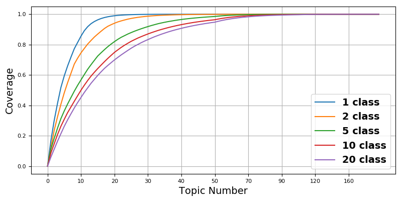
Figure 1: Topic coverage w.r.t number of used topics learned by iTM-VAE-HP.

Table 2: The posterior distribution of $\alpha$ learned by iTM-VAE-HP on subsets of 20News dataset.

#classes	$\gamma_{1}$	$\gamma_{2}$	$\mathbb{E}_{q(\alpha)}[\alpha]$
1	$16.88$	$4.58$	$3.68$
2	$23.03$	$3.68$	$6.25$
5	$31.43$	$2.88$	$10.93$
10	$39.64$	$2.69$	$14.71$
20	$48.91$	$2.98$	$16.39$

Table 2 reports the learned global variational parameter $\gamma_{1}$, $\gamma_{2}$ and the expectation of $\alpha$ given the variational poster $q(\alpha|\gamma_{1},\gamma_{2})$ on several subsets of 20News dataset, which contain $1$, $2$, $5$, $10$ and $20$ classes, respectively. We can see that, once the training is done, the variational posterior $q(\alpha|\gamma_{1},\gamma_{2})$ is very confident, and $\mathbb{E}_{q(\alpha|\gamma_{1},\gamma_{2})}[\alpha]$, the expectation of $\alpha$ given the variational posterior, is adjusted to the training set. For example, if the training set contains only $1$ class of documents, $\mathbb{E}_{q(\alpha|\gamma_{1},\gamma_{2})}[\alpha]$ after training is $3.68$, Whereas, when the training set consists of $10$ classes of documents, $\mathbb{E}_{q(\alpha|\gamma_{1},\gamma_{2})}[\alpha]$ after training is $14.71$. This indicates that iTM-VAE-HP can learn to adjust $\alpha$ to data, thus the number of discovered topics will adapt to data better. In contrast, for iTM-VAE-Prod (without the hyper-prior), when the decoder is strong, no matter how many classes the dataset contains, the number of topics will be constrained tightly due to the collapse-to-prior problem of AEVB, and KL-annealing and decoder regularizing tricks do not help much.

Figure 1 illustrates the training set coverage w.r.t the number of used topics when the training set contains $1$, $2$, $5$, $10$ and $20$ classes, respectively. Specifically, we compute the average weight of every topic on the training dataset, and sort the topics according to their average weights. The topic coverage is then defined as the cumulative sum of these weights. Figure 1 shows that, with the increasing of the number of classes, more topics are utilized by iTM-VAE-HP to reach the same level of topic coverage, which indicates that the model has the ability to adapt to data.

5.3 The Evaluation of HiTM-VAE

In this section, by comparing the topic coverage and sparsity of iTM-VAE-Prod and HiTM-VAE, we show that the hierarchical construction can help the model to learn more topics, and produce posterior topic proportions with higher sparsity.

The model configurations are the same for iTM-VAE-Prod and HiTM-VAE, except that $\alpha$ is set to $5$ and $20$ for iTM-VAE-Prod, and $\gamma=20,\alpha=5$ for HiTM-VAE. For HiTM-VAE, the corpus-level updates are done every $200$ epochs on 20News, and $20$ epochs on RCV1-V2.

As shown in Figure 2, HiTM-VAE can learn more topics than iTM-VAE-Prod ($\alpha=20$), and the sparsity of its posterior topic proportions is significantly higher. iTM-VAE-Prod ($\alpha=5$) has higher sparsity than iTM-VAE-Prod ($\alpha=20$). However, its sparsity is still lower than HiTM-VAE with the same document-level concentration parameter $\alpha$, and it can only learn a small number of topics, which means that there might exist rare topics that are not learned by the model. The comparison of HiTM-VAE and iTM-VAE-Prod ($\alpha=5$) shows that the superior sparsity not only comes from a smaller per-document concentration hyper-parameter $\alpha$, but also from the hierarchical construction itself.

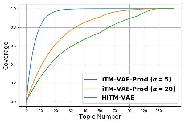
(a) Coverage

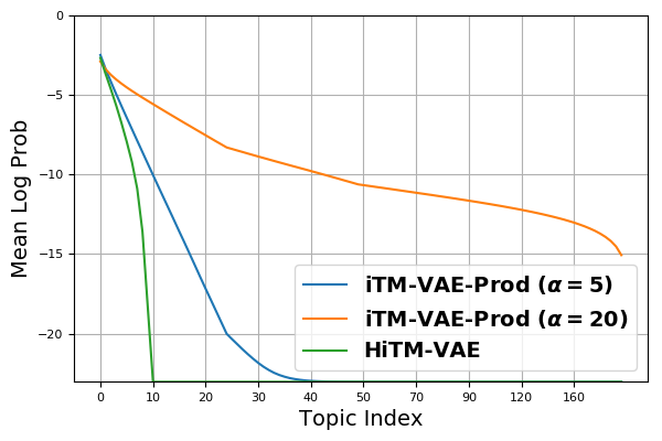
(b) Sparsity

Figure 2: Comparison of the topic coverage (a) and sparsity (b) between iTM-VAE-Prod ($\alpha=5$), iTM-VAE-Prod ($\alpha=20$) and HiTM-VAE ($\gamma=20$, $\alpha=5$). We can see that HiTM-VAE can simultaneously discover more topics and produce sparser posterior topic proportions.

6 Conclusion

In this paper, we propose iTM-VAE and iTM-VAE-Prod, which are nonparametric topic models that are modeled by Variational Auto-Encoders. Specifically, a stick-breaking prior is used to generate the atom weights of countably infinite shared topics, and the Kumaraswamy distribution is exploited such that the model can be optimized by AEVB algorithm. We also propose iTM-VAE-HP which introduces a hyper-prior into the VAE framework such that the model can adapt better to data. This technique is general and can be incorporated into other VAE-based models to alleviate the collapse-to-prior problem. To further diversify the document-specific topic distributions, we use a hierarchical construction in the generative procedure. And we show that the proposed model HiTM-VAE can learn more topics and produce sparser posterior topic proportions. The advantage of iTM-VAE and its variants over traditional nonparametric topic models is that the inference is performed by feed-forward neural networks, which is of rich representation capacity and requires only limited knowledge of the data. Hence, it is flexible to incorporate more information sources to the model, and we leave it to future work. Experimental results on two public benchmarks show that iTM-VAE and its variants outperform the state-of-the-art baselines.

References

- Archambeau et al. [2015] Cedric Archambeau, Balaji Lakshminarayanan, and Guillaume Bouchard. Latent ibp compound dirichlet allocation. IEEE transactions on pattern analysis and machine intelligence, 37(2):321–333, 2015.
- Bernardo and Smith [2001] José M Bernardo and Adrian FM Smith. Bayesian theory, 2001.
- Blei [2012] David M Blei. Probabilistic topic models. Communications of the ACM, 55(4):77–84, 2012.
- Blei et al. [2003] David M Blei, Andrew Y Ng, and Michael I Jordan. Latent dirichlet allocation. JMLR, 2003.
- Blei et al. [2006] David M Blei, Michael I Jordan, et al. Variational inference for dirichlet process mixtures. Bayesian analysis, 1(1):121–143, 2006.
- [6] Samuel R. Bowman, Luke Vilnis, Oriol Vinyals, Andrew M. Dai, Rafal Józefowicz, and Samy Bengio. Generating sentences from a continuous space. arXiv preprint arXiv:1511.06349.
- Card et al. [2017] Dallas Card, Chenhao Tan, and Noah A Smith. A neural framework for generalized topic models. arXiv preprint arXiv:1705.09296, 2017.
- Chen et al. [2017] Xi Chen, Diederik P. Kingma, Tim Salimans, Yan Duan, Prafulla Dhariwal, John Schulman, Ilya Sutskever, and Pieter Abbeel. Variational lossy autoencoder. 2017.
- Escobar and West [1995] Michael D Escobar and Mike West. Bayesian density estimation and inference using mixtures. Journal of the american statistical association, 90(430):577–588, 1995.
- Hinton [2006] Geoffrey E Hinton. Training products of experts by minimizing contrastive divergence. Neural Computation, 14(8), 2006.
- Hinton and Salakhutdinov [2009] Geoffrey E Hinton and Ruslan R Salakhutdinov. Replicated softmax: an undirected topic model. In NIPS, pages 1607–1614, 2009.
- Hoffman et al. [2010] Matthew Hoffman, Francis R. Bach, and David M. Blei. Online learning for latent dirichlet allocation. In NIPS. 2010.
- Ioffe [2017] Sergey Ioffe. Batch renormalization: Towards reducing minibatch dependence in batch-normalized models. 2017. URL http://arxiv.org/abs/1702.03275.
- Jang et al. [2017] Eric Jang, Shixiang Gu, and Ben Poole. Categorical reparameterization with gumbel-softmax. 2017. URL https://arxiv.org/abs/1611.01144.
- Kim and Sudderth [2011] Dae I Kim and Erik B Sudderth. The doubly correlated nonparametric topic model. In Advances in Neural Information Processing Systems, pages 1980–1988, 2011.
- Kingma and Ba [2015] Diederik Kingma and Jimmy Ba. Adam: A method for stochastic optimization. In ICLR, 2015.
- Kingma and Welling [2014a] Diederik Kingma and Max Welling. Efficient gradient-based inference through transformations between bayes nets and neural nets. In ICML, pages 1782–1790, 2014a.
- Kingma and Welling [2014b] Diederik P Kingma and Max Welling. Auto-encoding variational bayes. In ICLR, 2014b.
- Kumaraswamy [1980] Ponnambalam Kumaraswamy. A generalized probability density function for double-bounded random processes. Journal of Hydrology, 46(1-2):79–88, 1980.
- Larochelle and Lauly [2012] Hugo Larochelle and Stanislas Lauly. A neural autoregressive topic model. In NIPS, 2012.
- Lau and Baldwin [2016] Jey Han Lau and Timothy Baldwin. The sensitivity of topic coherence evaluation to topic cardinality. In NAACL HLT, pages 483–487, 2016.
- Lau et al. [2014] Jey Han Lau, David Newman, and Timothy Baldwin. Machine reading tea leaves: Automatically evaluating topic coherence and topic model quality. In EACL, pages 530–539, 2014.
- Lim et al. [2016] Kar Wai Lim, Wray Buntine, Changyou Chen, and Lan Du. Nonparametric bayesian topic modelling with the hierarchical pitman–yor processes. International Journal of Approximate Reasoning, 78:172–191, 2016.
- Miao et al. [2016] Yishu Miao, Lei Yu, and Phil Blunsom. Neural variational inference for text processing. In ICML, pages 1727–1736, 2016.
- Miao et al. [2017] Yishu Miao, Edward Grefenstette, and Phil Blunsom. Discovering discrete latent topics with neural variational inference. In ICML, 2017.
- Mnih and Gregor [2014] Andriy Mnih and Karol Gregor. Neural variational inference and learning in belief networks. In ICML, 2014.
- Murphy [2012] Kevin P Murphy. Machine learning: a probabilistic perspective. MIT press, 2012.
- Nalisnick and Smyth [2017] Eric Nalisnick and Padhraic Smyth. Stick-breaking variational autoencoders. In ICLR, 2017.
- Newman et al. [2010] David Newman, Jey Han Lau, Karl Grieser, and Timothy Baldwin. Automatic evaluation of topic coherence. In NAACL HLT, pages 100–108, 2010.
- Putthividhy et al. [2010] Duangmanee Putthividhy, Hagai T Attias, and Srikantan S Nagarajan. Topic regression multi-modal latent dirichlet allocation for image annotation. In CVPR, pages 3408–3415. IEEE, 2010.
- Ranganath et al. [2014] Rajesh Ranganath, Sean Gerrish, and David Blei. Black box variational inference. In AISTATS, 2014.
- Rasiwasia and Vasconcelos [2013] Nikhil Rasiwasia and Nuno Vasconcelos. Latent dirichlet allocation models for image classification. IEEE transactions on pattern analysis and machine intelligence, 35(11):2665–2679, 2013.
- Rezende et al. [2014] Danilo Jimenez Rezende, Shakir Mohamed, and Daan Wierstra. Stochastic backpropagation and variational inference in deep latent gaussian models. In ICML, 2014.
- Rogers et al. [2005] Simon Rogers, Mark Girolami, Colin Campbell, and Rainer Breitling. The latent process decomposition of cdna microarray data sets. IEEE/ACM TCBB, 2(2):143–156, 2005.
- Sethuraman [1994] Jayaram Sethuraman. A constructive definition of dirichlet priors. Statistica sinica, 1994.
- Sønderby et al. [2016] Casper Kaae Sønderby, Tapani Raiko, Lars Maaløe, Søren Kaae Sønderby, and Ole Winther. Ladder variational autoencoders. In Advances in Neural Information Processing Systems, pages 3738–3746, 2016.
- Srivastava and Sutton [2017] Akash Srivastava and Charles Sutton. Autoencoding variational inference for topic models. In ICLR, 2017.
- Teh et al. [2006] Yee Whye Teh, Michael I Jordan, Matthew J Beal, and David M Blei. Hierarchical dirichlet processes. Journal of the American Statistical Association, 101(476):1566–1581, 2006.
- Wang et al. [2011] Chong Wang, John Paisley, and David Blei. Online variational inference for the hierarchical dirichlet process. In AISTATS, pages 752–760, 2011.
- Wei and Croft [2006] Xing Wei and W Bruce Croft. Lda-based document models for ad-hoc retrieval. In SIGIR, 2006.