Modeling dynamical phonon fluctuations across the magnetically driven polaron crossover
in the manganites

Abstract

We investigate the dynamical structure factor associated with lattice fluctuations in a model that approximates the manganites. It involves electrons strongly coupled to core spins, and to lattice distortions, in a weakly disordered background. This model is solved in the adiabatic limit in two dimensions via Monte Carlo, retaining all the thermal fluctuations. In the metallic phase near the polaronic crossover this approach captures the effect of thermally induced polaron formation, and their short range correlation, on the electronic spectral functions. The dynamical fluctuations of the optical and acoustic phonon modes are computed at a ‘one loop’ level by calculating the electronic polarisability in the the thermally fluctuating backgrounds, and solving the phonon Dyson equations in real space. We present phonon lineshapes across the ferromagnet to paramagnet thermal transition and correlate them with changing electronic properties. We compare our results with inelastic neutron scattering data on the metallic manganites, and also predict what one may find in the more insulating phases.

I Introduction

The dispersion of phonons in metals has a ‘direct’ part, determined by the interactions between the ions, and an indirect part determined by electron-phonon coupling and the electronic polarisability phon . The damping similarly can arise from phonon-phonon interaction - related to nonlinearities in the inter-ionic potential, or the polarisability - via particle-hole pair creation. Phonon physics associated with ionic interactions is well understood but the effects arising out of a non trivial polarisability, in correlated electron systems, have generated a new list of questions.

Many electronic systems have now been shown to exhibit behaviour that differs widely from the band picture dag . In particular correlation effects give rise to competing ordered phases, short range order, and sometimes a pseudogapped electronic spectrum - widely at variance with band theoryman ; cup . The short range order gives a characteristic momentum dependence to electronic properties, the pseudogap generates a new frequency scale, and temperature plays an important role in the evolution of both these features. The electronic polarisability $\Pi({\bf q},\Omega,T)$, where ${\bf q}$ is the momentum, $\Omega$ the frequency, and $T$ the temperature, becomes a non trivial function - very distinct from its weak coupling Lindhard counterpart. It is no wonder that phonons in these correlated systems show a very rich behaviour.

For example, recent experiments weber1 ; weber2 ; weber3 reveal the impact of short-range charge order (CO), and an electronic pseudogap, on the softening and broadening of the bond stretching phonons in the manganites for momenta near the CE ordering wavevector. Similar effects on phonons have been observed in underdoped cupratesreznik ; dean , possibly owing to stripe order. In fact phonon properties near ${\bf q}\sim(\frac{1}{4},\frac{1}{4},0)$, the CE ordering wavevector, in manganites are very similar to that in cuprates at ${\bf q}\sim(\frac{1}{4},0,0)$. In the nickelateskajimoto , inelastic neutron scattering reveals strong softening and branch-splitting of longitudinal optical (LO) phonons. Strong phonon renormalizations have also been reported in doped bismuthatesbraden possibly due to their coupling to interplanar charge fluctuations.

There are two distinct scenarios to consider when approaching these problems. (a) Situations where the electron correlations arise from inter-electron interactions - and the phonons are only weakly coupled to the electrons, and (b) where electron-phonon interaction is itself responsible (if only in part) for features in the electronic spectrum. Category (a), possibly appropriate to the cupratescup , requires a solution of the interacting electron problem and then use of the resulting $\Pi({\bf q},\Omega)$ to determine the phonon self-energy. Category (b) requires an “ab initio” handling of lattice distortions, and is pertinent to the manganitesman .

This paper is focused on understanding phonons in a model that approximates the manganites. We will consider models in category (a) elsewhere. To set the stage we quickly recapitulate the electronic observations in the intermediate coupling manganites, and the recent results on phonon spectra.

The manganites A_1-xB_xMnO₃, where A is trivalent and B is divalent, involve $e_{g}$ electrons Hund’s coupled to $t_{2g}$ based core spins, and to Jahn-Teller (JT) distortions of the MnO₆ octahedraman ; millis1 . The Hund’s coupling promotes ferromagnetism (and extended electronic states) while the JT coupling favours polaron formation (and electron localisation). The bandwidth and carrier density can be tuned via choice of the A and B ions, and $x$. A material that is a ferromagnetic metal (FM) at low temperature can show polaronic signatures with increasing temperature as spin randomness reduces the effective bandwidth. In fact it can cross over to a paramagnetic insulator (PI) across the magnetic transition. There is naturally a drastic change in the electronic spectra with temperature in this parameter window.

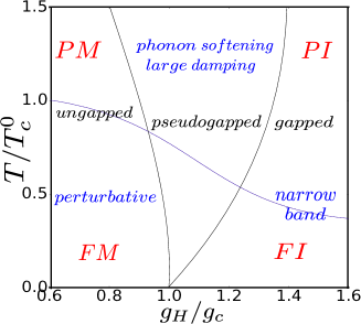
Figure 1: Phonon ‘phase diagram’ for the 2D double exchange Holstein model near half filling for varying coupling and temperature. We normalize coupling $g_{H}$ by the zero temperature critical coupling for polaron formation $g_{c}$ and temperature by the ferromagnetic transition temperature at weak coupling $T^{0}_{c}=2\Omega_{0}$, where $\Omega_{0}$ is the bare Holstein frequency. FM and PM denote the ferromagnetic and paramagnetic metal phases, similarly FI and PI are ferro and para insulating phases. The phonon regimes are indicated in blue.

Inelastic neutron scattering has uncovered the following phonon features in this regime.

1. The Mn-O bond stretching phonons along the (110) direction in the bilayer manganite La_1.2Sr_1.8Mn₂O₇ soften and broaden close to the CE ordering wavevector in the low temperature ($\sim 10$K) metallic phaseweber1 .

2. A similar effect is observed in the 3D compound La_0.7Sr_0.3MnO₃ for the transverse acoustic phonons, on heating through the Curie temperature $T_{c}\sim 350$K weber2 .

3. In the charge and orbital ordered bilayer manganite LaSr₂Mn₂O₇, one sees a reduction in broadening and softening of low-energy acoustic phonons on cooling below $T_{CO}\sim 225$K weber3 .

We wish to address these issues, by first solving the appropriate electronic problem. To retain the key qualitative features of manganite physics, and also to access large spatial scales, we study a two dimensional model of electrons Hund’s coupled to core spins and to lattice distortions via a Holstein coupling. We retain weak disorder in the model - to mimic the effect of cation disorder in the doped materials. This problem is solved via a Monte Carlo method in real space, and the electronic polarisability that emerges is used to compute the phonon spectra.

We list our main results below. In our notation $g_{H}$ is the Holstein coupling and $g_{c}$ its value for the adiabatic polaron transition.

1. At $g_{H}\ll g_{c}$ the ground state is a ferromagnetic metal at low temperature, with dispersive phonons that show a Kohn anomaly close to half filling. With increasing temperature spin disorder and thermally induced lattice distortions create a a mild electronic pseudogap, and also broaden the phonons considerably.

2. For $g_{H}\lesssim g_{c}$ the interplay of electron-phonon coupling and disorder localises the phonons. The phonon spectrum, as a result, is quite incoherent. The electronic density of states features a pseudogap. Thermal effects further accentuate lifetimes.

3. For $g_{H}\gtrsim g_{c}$ the ground state is a ferromagnetic insulator. The electronic spectrum is gapped and phonon band is narrow, with bandwidth limited lifetimes. This is related to emergent short-range order in the background. On heating past the ferromagnetic $T_{c}$, phonon lifetimes pick up.

Fig.1 summarizes our findings regarding thermodynamic phases (indicated in red), electronic states (in black) and phonon regimes (in blue). It’s discussed in detail later in context of the thermal physics. In reporting the results, we first focus on the ground state. The next section exhibits our findings about the thermal physics. This is followed by the discussion section, summarizing the results and making a qualitative correspondence with experiments, and a concluding section.

II Model and method

We study the disordered Holstein-double exchange (d-HDE) model, coupled to acoustic phonons on a two-dimensional square lattice. The full problem has three parts- (i) the ‘d-HDE’ part - electrons coupled to optical phonons and ‘core’ spins, in a weakly disordered background, (ii) an acoustic phonon mode, and (iii) ‘weak’ coupling between the acoustic phonons and electrons. The total Hamiltonian is:

$$H_{tot}=H_{1}+H_{2}+H_{3}$$ (1)

The Hamiltonian for the d-HDE part is-

$$H_{1} = \sum_{<ij>\sigma}t_{ij}c^{\dagger}_{i\sigma}c_{j\sigma}-J_{H}\sum_{i}\vec{S}_{i}.\vec{\sigma}_{i}+\sum_{i}(\epsilon_{i}-\mu)n_{i}$$ (3)

$$~{}~{}-g_{H}\sum_{i}n_{i}x_{i}+\sum_{i}(\frac{p^{2}_{i}}{2M}+\frac{1}{2}Kx^{2}_{i})$$

Here, $t_{ij}$’s are the hopping amplitudes. We study a nearest neighbour model with $t=1$ for a nearly commensurate density, viz. $n=0.40$. $K$ and $M$ are the stiffness constant and mass, respectively, of the optical phonons, and $g$ is the electron-phonon coupling constant. We set $K=1$. In this paper, we report studies for $\Omega_{0}=\sqrt{K/M}=0.05$, which is a reasonable value for real materials. $\vec{S}_{i}$’s are ‘core spins’, assumed to be large and classical. $\epsilon_{i}$ is a quenched binary disorder with zero mean and value $\pm\Delta$. The chemical potential $\mu$ is varied to maintain the electron density at the required value. We’ll work in the extreme Hund’s coupling limit $J_{H}/t\rightarrow\infty$. This effectively enslaves the electrons spins to the core spin orientation and one obtains an effectively spinless, hopping disordered model-

$$H_{1} = \sum_{<ij>}t_{ij}{\gamma}^{\dagger}_{i}{\gamma}_{j}+\sum_{i}(\frac{p^{2}_{i}}{2M}+\frac{1}{2}Kx^{2}_{i})$$ (4)

$$+ \sum_{i}(\epsilon_{i}-\mu-g_{H}x_{i})n_{i}$$

The hopping amplitude depends on spin orientation via the relation-

$$t_{ij}/t=cos\frac{\theta_{i}}{2}cos\frac{\theta_{j}}{2}+isin\frac{\theta_{i}}{2}sin\frac{\theta_{j}}{2}e^{i(\phi_{i}-\phi_{j})}$$ (5)

where the $\theta_{i}$ and $\phi_{i}$ are, respectively, the polar and azimuthal angles of the core spins $\vec{S}_{i}$. The Hamiltonian for the bare acoustic phonons is-

$$H_{2}=\sum_{\vec{q}}\omega_{\vec{q}}a^{\dagger}_{\vec{q}}a_{\vec{q}}$$ (6)

with the bare dispersion given by the equation-

$$\omega^{2}_{\vec{q}}=\frac{2\kappa}{\mu}(2-cos(q_{x})-cos(q_{y}))$$ (7)

We choose $\kappa=1.0$ and $\mu=2500$ as parameters. This ensures that the maximum of the acoustic branch is comparable to the bare optical mode frequency at the zone boundary.

The coupling between the acoustic phonons and electrons is the third part of the Hamiltonian-

$$H_{3}=ig_{ac}\sum_{\vec{k}\vec{q}}\frac{|\vec{q}|}{\sqrt{2\mu\omega_{q}}}(a_{\vec{q}}-a^{\dagger}_{-\vec{q}})c^{\dagger}_{\vec{k}+\vec{q}}c_{\vec{k}}$$ (8)

We’ve written the parts $H_{2}$ and $H_{3}$ in momentum space for simplicity, but the actual calculations using them have been implemented in real space. This has the advantage of capturing spatial correlations amongst static distortions and the core spin angles at finite temperature.

We solve the problem hierarchically. First, the d-HDE problem is tackled in the adiabatic regime (assuming $\Omega_{0}/t\rightarrow 0$). The $H_{1}$ part in the model leads to the action

$$S = \int_{0}^{\beta}d\tau[\sum_{ij}\bar{\psi_{i}}\{(\partial_{\tau}+\epsilon_{i}-\mu)\delta_{ij}-t_{ij}\}\psi_{j}$$

$$~{}~{}+\sum_{i}\bar{\Phi}_{i}(\partial_{\tau}+\Omega_{0})\Phi_{i}-~{}g_{H}\sqrt{\frac{\Omega_{0}}{2K}}\sum_{i}(\bar{\Phi}_{i}+\Phi_{i}){\bar{\psi}_{i}}\psi_{i}]$$

Here $\psi_{i}$ and $\phi_{i}$ are the fermion and coherent state Bose fields respectively. $\beta$ denotes the inverse temperature, and we use units where $k_{B}=1$, $\hbar=1$. The relation between the real and coherent state fields is

$$x_{i}=\sqrt{\frac{1}{2M\Omega_{0}}}(\Phi_{i}+\bar{\Phi}_{i})$$ (10)

In quantum Monte Carlo (QMC) QMC , one ‘integrates out’ the fermion fields to construct the effective bosonic action. The equilibrium configurations $\Phi_{i}(\tau)$ of that theory are obtained via sampling. Physical correlators are then computed as averages with respect to these $\Phi_{i}(\tau)$ configurations. Within DMFT DMFT one maps the original action in Eq.(2) to an impurity problem, with parameters determined through a self-consistency condition.

In the adiabatic limit, or using the static path approximation (SPA) strategy, one treats the $x_{i}$ as classical fields, neglecting their imaginary time dependence. This corresponds to $M\rightarrow\infty$ for a fixed $K$. In addition, the $\theta_{i}$ and $\phi_{i}$ angles also fluctuate at finite temperature. Our method retains the quantum character of lattice vibrations perturbatively.

The full action containing the electrons, displacement fields and core spins can be rewritten in frequency space as-

$$S = S_{ph}+S_{f}$$

$$S_{ph} = \frac{1}{2}\sum_{i,m}\bar{x}_{im}(M\omega_{m}^{2}+K)x_{im}$$ (11)

$$S_{f} = \sum_{i,j,\alpha,\beta}\bar{\psi}_{i\alpha}[(-i\omega_{\alpha}+\epsilon_{i}-\mu)\delta_{ij}\delta_{\alpha\beta}-t_{ij}\delta_{\alpha\beta}$$ (13)

$$~{}~{}~{}~{}~{}~{}~{}~{}~{}~{}~{}~{}~{}~{}~{}~{}~{}~{}-g_{H}\sqrt{\beta}x_{i,\alpha-\beta}\delta_{ij}]\psi_{j\beta}$$

where $\alpha$ and $\beta$ are fermionic Matsubara frequencies, $m$ is a Bose frequency. To get the partition function, one integrates over $\psi_{i\alpha}$, $x_{i0}$ and the $x_{im}$ fields and of course, the angular variables hidden in $t_{ij}$.

The next step is to separate the Bose field into zero and non-zero Matsubara modes. We write $S=S_{0}+S_{1}$ where the first part contains fermions coupling only to the zero frequency (static) mode and the second, the finite modes. We can formally ‘diagonalize’ the fermions in presence of the static mode to write $S_{0}$ as-

$$S_{0}={\sum_{l,\alpha}\bar{\xi}_{l,\alpha}(-i\omega_{\alpha}+\epsilon_{l})\xi_{l,\alpha}}+\frac{1}{2}K\sum_{i}x^{2}_{i0}$$ (14)

where $\xi$’s correspond to the fermionic eigenmodes in the $\{x_{i0},\theta_{i},\phi_{i}\}$ background. $S_{0}$ defines the static path approximation (SPA) action.

The eigenvalues ($\epsilon_{l}$’s ) depend non-trivially on the $\{x_{i0},\theta_{i},\phi_{i}\}$ background. To obtain the effective zero mode distribution $P\{x_{i0},\theta_{i},\phi_{i}\}$, one has to integrate out the fermions. At the SPA level, there exists an effective Hamiltonian $H_{eff}$, depending on $\{x_{i0},\theta_{i},\phi_{i}\}$, for the fermions and the distribution can be formally written as-

$$H_{eff} = \sum_{<ij>}t_{ij}{\gamma}^{\dagger}_{i}{\gamma}_{j}-g\sum_{i}n_{i}x_{i0}$$ (15)

$$P\{x_{i0},\theta_{i},\phi_{i}\} = Tr_{{\gamma},{\gamma}^{\dagger}}e^{-\beta(H_{eff}+{1\over 2}Kx_{i0}^{2})}$$

Around the SPA action, we set up a cumulant expansion of $S_{1}$. Owing to the disparate timescales of the optical phonons and electrons, we attempt a sequential integrating out. First, the fermions are traced out and one obtains the following expression for $S_{1}$ in terms of the $x_{i}(i\Omega_{m})$:

$$S_{1} = S^{\prime}_{ph}-Trln[\beta((-i\omega_{\alpha}+\epsilon_{i}-\mu)\delta_{ij}\delta_{\alpha\beta}$$

$$~{}~{}~{}~{}~{}~{}~{}~{}~{}~{}~{}~{}~{}~{}~{}-t_{ij}\delta_{\alpha\beta}-g_{H}\sqrt{\beta}x_{i,\alpha-\beta}\delta_{ij})]$$

$$S^{\prime}_{ph} = \frac{1}{2}\sum_{i,m\neq 0}\bar{x}_{im}(M\omega_{m}^{2}+K)x_{im}$$ (16)

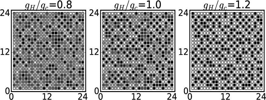
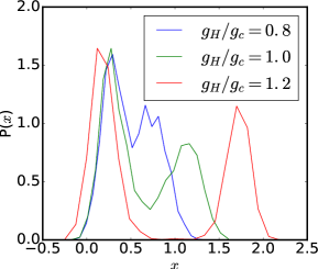
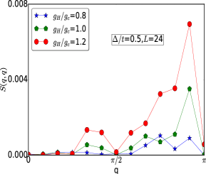
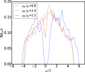
Figure 2: Top row: Snapshots of static optical phonon backgrounds in the ground state for weak ($g/g_{c}=0.8$, left panel), intermediate ($g/g_{c}=1.0$, middle panel) strong ($g/g_{c}=1.2$, right panel) couplings. We see a gradually developing short-range ($\pi,\pi$) correlation on moving from left to right, bottom row: a) left panel- Distribution of static distortions $P(x)$ for three couplings. We see a weak bimodality transforming to a prominent two-peak distribution at strong coupling, b) middle panel- static phonon structure factor along the BZ diagonal $S(q,q)$ for the same coupings, confirming features seen in lattice backgrounds, c) right panel- electronic density of states $N(\omega)$ from weak to strong coupling. We see an evolution from tight-binding like spectrum to a small hard-gap DoS at strong coupling through a pseudogap regime.

Analytic determination of the trace is impossible beyond weak coupling. Our method constitutes of expanding the trace in finite frequency $x_{i}$ modes upto Gaussian level. Physically, we assume that the quantum fluctuations are small in amplitude, controlled by a low $\gamma=\Omega_{0}/t$ ratio. Retaining only quadratic terms in the dynamic modes allows us to analytically integrate them out later. An analogous strategy has been explored within DMFT beforemillis2 .

The method is obviously perturbative in $\gamma$ as we diagonalize the fermions in presence of static distortions and evaluate correlation functions on this ‘frozen’ background, which enter as coefficients of the quadratic Bose term for finite frequencies. After re-exponentiating this term (in the Gaussian approximation spirit), the new partition function becomes-

$$Z=\int[D\bar{x}][Dx][D\theta][D\phi][D\bar{\xi}][D\xi]e^{-(S_{0}+S_{1})}$$ (17)

where

$$S_{0} = {\sum_{l,\alpha}\bar{\xi}_{l,\alpha}(-i\omega_{\alpha}+\epsilon_{l})\xi_{l,\alpha}}+\frac{1}{2}Kx_{i0}^{2}$$ (18)

$$S_{1} = {\sum_{i,j,m>0}\bar{x}_{im}[(M\omega^{2}_{m}+K)\delta_{ij}+{g_{H}^{2}}\Pi_{ij}^{m}(\{x_{i,0},\theta_{i},\phi_{i}\})]x_{jm}}$$

$\Pi_{ij}^{m}$ is a one-loop fermion polarization correcting the free Bose propagators. The expression for this is

$$\Pi_{ij}^{m}(\{x_{i0},\theta_{i},\phi_{i}\})=\frac{1}{\beta}\sum_{\alpha}G_{ij}^{m}G_{ji}^{\alpha-m}$$ (19)

$G_{ij}^{m}$’s are Matsubara components of real-space fermion Green’s functions computed in an arbitrary static background. One can write a spectral representation of this as follows-

$$G^{m}_{ij}(\{x_{i0},\theta_{i},\phi_{i}\})=\sum_{n}\frac{u_{in}\bar{u}_{jn}}{i\omega_{m}-\epsilon_{n}}$$ (20)

where $u_{in}$ is amplitude at site $i$ for the $n$th eigenstate of the SPA Hamiltonian and $\epsilon_{n}$’s are the corresponding eigenvalues.

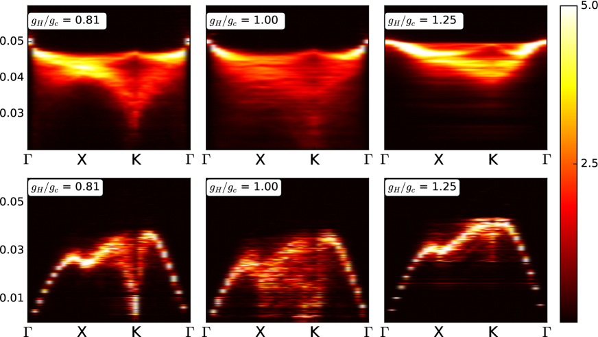
Figure 3: Spectral distribution of the optical (top panel) and acoustic (bottom panel) phonon Green’s function for varying $g_{H}$ in the ground state. The trajectory chosen along BZ is $(0,0)\rightarrow(\pi,0)\rightarrow(\pi,\pi)\rightarrow(0,0)$. Coupling increases along the horizontal axis in the following sequence (from left to right)- $g_{H}/g_{c}=(0.81,1.00,1.25)$. The critical coupling at this density is $g_{c}=1.60$. For the acoustic plots, $g_{ac}=g_{H}$.

If we integrate out the finite frequency Bose modes (in $S_{1}$), a new $x_{i0}$ theory emerges. One can treat this resulting action with classical Monte Carlo (MC) simulations to obtain the optimal background in which the fermions move. This basically means that at each MC update, one uses the sum of the SPA free energy and the contribution from the finite frequency Gaussian fluctuation, to compute the update probability.

The coefficient of the quadratic Bose term of $S_{1}$ in (13) defines the inverse propagator $(D^{-1})_{ij,m}$ for the renormalized optical phonons. One can view the $\Pi^{m}_{ij}$ as a self-energy for the phonons in real space, correcting the bare propagator. To get the renormalized Green’s function, one needs to solve a Dyson’s equation on the lattice with possibly inhomogeneous backgrounds.

$$[D]^{-1}_{ij}(\omega)=[D]^{-1}_{0,ij}(\omega)+g_{H}^{2}[\Pi]_{ij}(\omega)$$ (21)

Here the bare phonon propagator $D^{-1}_{0,ij}$ is defined through the equation-

$$[D]^{-1}_{0,ij}(\omega)=(M\omega^{2}-K)\delta_{ij}$$ (22)

where we have analytically continued the Green’s functions to real frequency and $D^{-1}_{0,ij}$ denotes the inverse propagator for the bare phonon. This involves a calculation that grows as $O(N^{4})$ with increasing lattice size $N$. For lattices of size 24$\times$24, this computation was implemented.

Next, we consider the acoustic phonons. As commented earlier, we rewrite the parts $H_{2}$ and $H_{3}$ in real space-

$$H_{2} = \sum_{ij}M_{ij}a^{\dagger}_{i}a_{j}$$

$$H_{3} = \sum_{ij\vec{q}}\frac{ig_{ac}|\vec{q}|}{\sqrt{2\mu\omega_{\vec{q}}}}(a_{j}e^{i(\vec{r}_{i}-\vec{r}_{j}).\vec{q}}-h.c.)c^{\dagger}_{i}c_{i}$$ (23)

The bare phonon is found by just inverting the matrix $M_{ij}$ in $H_{2}$. Its explicit form is given by-

$$[\tilde{D}]_{0,ij}(\omega)=\frac{e^{-i(\vec{r}_{i}-\vec{r}_{j}).\vec{q}}}{\omega-\omega_{\vec{q}}+i\eta}-\frac{e^{-i(\vec{r}_{i}-\vec{r}_{j}).\vec{q}}}{\omega+\omega_{\vec{q}}-i\eta}$$ (24)

where $\eta$ is a positive infinitesimal. The coupling $H_{3}$ gives a self-energy contribution, which can be written as a matrix product-

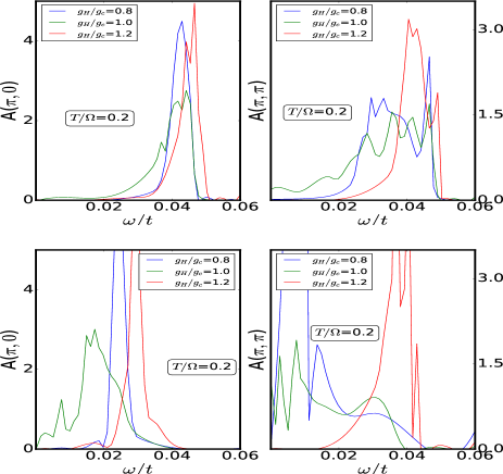
Figure 4: Momentum resolved spectral functions $A(\pi,0)$ and $A(\pi,\pi)$ (left and right panels) of the optical (top row) and acoustic (bottom row) phonons for varying $g_{H}/g_{c}=(0.8,1.0,1.2)$. The relevant couplings along with color codes are listed.

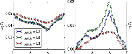
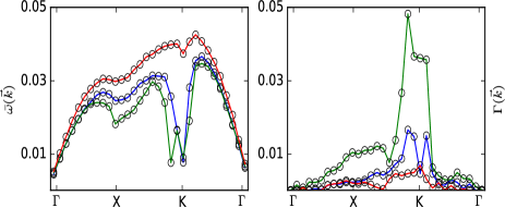
Figure 5: Fitting of optical (top panel) and acoustic (bottom panel) phonon spectra for the ground state in terms of mean frequencies ($\bar{\omega}(\vec{k})$ and linewidths ($\Gamma(\vec{k})$ throughout the BZ trajectory $(0,0)\rightarrow(\pi,0)\rightarrow(\pi,\pi)\rightarrow(0,0)$. The relevant couplings are listed along with color codes.

$$\tilde{\Pi}_{ab}={A}_{ai}{\Pi}_{ij}{B}_{jb}$$ (25)

where $\Pi_{ij}$ is the same as in equation (14). The matrices sandwiched to the left and right are comprised of weighted form factors. They have the following expressions-

$$A_{ai} = \sum_{\vec{q}}\frac{|\vec{q}|}{\sqrt{2\mu\omega_{\vec{q}}}}e^{i(\vec{r}_{i}-\vec{r}_{a}).\vec{q}}$$

$$B_{jb} = \sum_{\vec{{q}^{\prime}}}\frac{|\vec{{q}^{\prime}|}}{\sqrt{2\mu\omega_{\vec{{q}^{\prime}}}}}e^{i(\vec{r}_{j}-\vec{r}_{b}).\vec{{q}^{\prime}}}$$ (26)

Finally, a Dyson equation is solved (in real space) as in the optical phonon case-

$$[\tilde{D}]^{-1}_{ab}(\omega)=[\tilde{D}]^{-1}_{0,ab}(\omega)-\tilde{\Pi}_{ab}(\omega)$$ (27)

III Results on the ground state

We organize the results as follows. First, the optimal static background features are shown. These include individual MC snapshots, the distribution of static optical phonon distortions $P(x_{0})$ the static phonon structure factor along the BZ diagonal ($S(q,q)$) and electronic density of states (DoS) in the ground state. Next, the spectral maps in ($\vec{k},\omega$) space of the optical and acoustic phonon propagators, calculated with the full frequency dependent $\Pi_{ij}(\omega)$, are featured. These spectra were calculated for moderately large sizes (24$\times$24). To enable a closer look into phonon properties, we plot the lineshapes for a couple of high symmetry $k$-points in the BZ - ($\pi,0$) and ($\pi,\pi$).

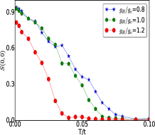
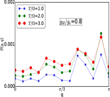
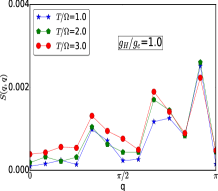
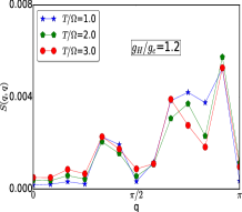
Figure 6: Ferromagnetic structure factor $S(0,0)$ (top left) for three couplings of interest and static phonon structure factors $S(q,q)$ along the diagonal of BZ for three temperatures $T/\Omega=(1.0,2.0,3.0)$ in subsequent panels.

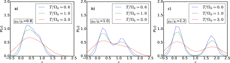
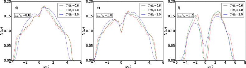
Figure 7: Top row: The distribution of static optical mode distortions ($P(x)$) across three coupling windows a) weak ($g_{H}/g_{c}=0.8$), b) intermediate ($g_{H}/g_{c}=1.0$) and c) strong ($g_{H}/g_{c}=1.2$). The weak bimodality in the ground state at weak coupling smoothens out due to thermal fluctuations. At intermediate coupling, bimodality remains upto mild heating ($T/\Omega_{0}\sim 1.0$). The strong coupling distribution is bimodal even upto $T/\Omega_{0}=3.0$. Bottom row: electronic DoS across the same couplings- d) a mild pseudogap seen at weak coupling for high $T$, e) intermediate coupling features gradually diminishing pseudogaps on heating, f) strong coupling DoS is gapped at low $T$, has more robust pseudogap feature on heating.

Given that it’s difficult to interpret these lineshapes directly, we’ve extracted mean frequencies and widths for the entire optical and acoustic phonon spectra. We also attempt to make a connection between the observed phonon features and the corresponding electronic physics on the static backgrounds. The quantity which affects phonon features directly in our theory is the polarization $\Pi_{ij}(\omega)$. We don’t provide any analysis of these in the present paper, but interpreting them is currently in progress.

III.1 Backgrounds

In this part, we show quantities characterizing the static optical mode which controls most of the phonon physics. First, the actual MC snapshots of lattice distortions are featured, followed by probability distribution of these ($P(x)$), which indicate polaron formation. Next, the structure factor along the BZ diagonal shows emergence of short-range correlations near ($\pi,\pi$). Finally, the electronic DoS in the ground state are exhibited, that show a gap formation at strong coupling.

The MC snapshots, shown in top row of Fig.2, reveal static phonon correlations across various coupling windows. These pictures are representative of the ground state ($T/\Omega_{0}=0.2$). One sees a gradual improvement of $(\pi,\pi)$ correlations amongst the distortions as we move from weak to strong coupling (left to right). However, at weaker $g_{H}/g_{c}$, the features are much less underlined. In the clean Holstein model, the strong coupling state is supposed to be ordered, at least close to half-filling. Here, the weak binary disorder has the effect of destroying that, but short range correlations persist. The temperature scale for killing off these effects is set by $T_{CO}\sim\frac{t^{2}}{E_{p}}$.

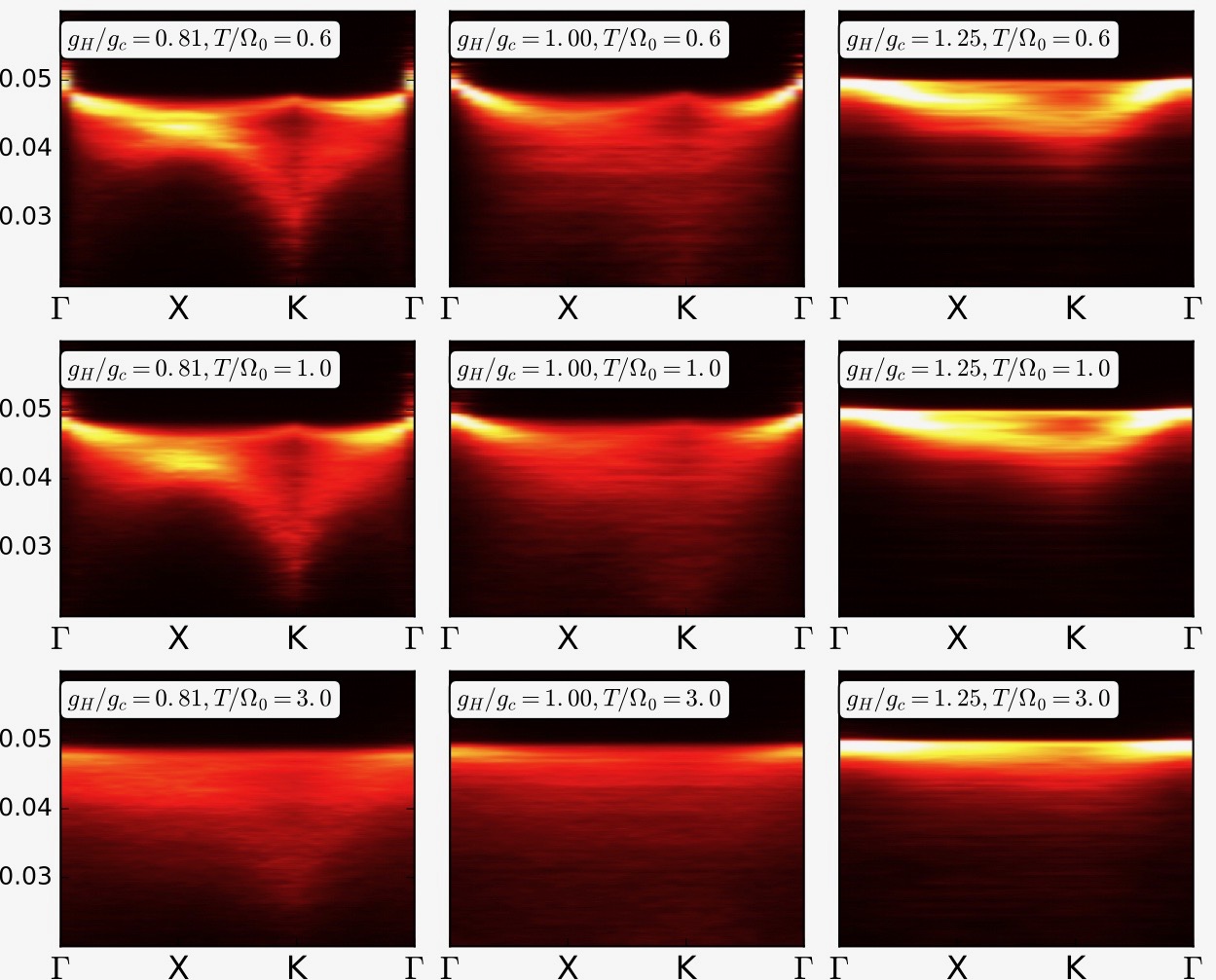
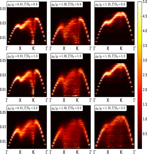
Figure 8: Left set: Spectral distribution of the optical phonon Green’s function for varying $g_{H}$ and temperature. The trajectory chosen along BZ is $(0,0)\rightarrow(\pi,0)\rightarrow(\pi,\pi)\rightarrow(0,0)$. Coupling increases along the horizontal axis in the following sequence (from left to right)- $g_{H}/g_{c}=(0.81,1.00,1.25)$. Temperature varies form top to bottom- $T/\Omega_{0}=(0.6,1.0,3.0)$. The critical coupling at this density is $g_{c}=1.60$. Right set: Spectral distribution of the acoustic phonon Green’s function for varying $g_{H}$ and temperature. The trajectory chosen along BZ is $(0,0)\rightarrow(\pi,0)\rightarrow(\pi,\pi)\rightarrow(0,0)$. Coupling increases along the horizontal axis in the following sequence (from left to right)- $g_{H}/g_{c}=(0.81,1.00,1.25)$. Temperature varies form top to bottom- $T/\Omega_{0}=(0.6,1.0,3.0)$. The critical coupling at this density is $g_{c}=1.60$. For these plots, $g_{ac}=g_{H}$.

The bottom row of Fig.2 shows first the distribution of static distortions. At the weakest coupling, a hint of bimodality is seen amidst a generally broad picture. On going closer to the actual crossover ($g_{H}/g_{c}=1.0$), a genuine two-peak distibution emerges with more weight on the smaller $x$ value. At strong coupling, a clear gap separates the two modes. The effect of disorder is to enhance polaronic features at weaker couplings and broaden the peaks at strong coupling.

Next, we come to static phonon structure factor $S(q,q)$ in the ground state, from which the conclusions drawn from individual configurations can be further corroborated. Close to the zone boundary, we see mild peaks, whose weights become prominent at strong coupling.

Finally, the electronic DoS also responds to the polaronic transition directly. We have a tight-binding like spectrum at weak coupling. The phonon induced renormalizations are small. Close to the transition, the behaviour changes qualitatively and a pseudogap emerges. At even higher couplings, polarons tend to order. As a result, we see formation of a small, hard gap.

III.2 Overview of phonon modes

In Fig.3, we exhibit the spectral maps of the optical and acoustic phonons in various coupling regimes. We already depicted such maps in our previous worksauri on the clean Holstein model. The first row is depicting optical phonons on the ground state. Below $g_{H}=g_{c}$, the mode is fairly sharp except in the vicinity of $(\pi,0)$, and most noticeably around $(\pi,\pi)$, where it also splits and softens to some degree. We ascribe this behaviour to the proximity to a nesting instability ($n=0.4$ is close to half-filling). Compared to the clean Holstein problem, the broadenings are considerably large in the present case. The reason is the presence of weak binary disorder, which also affects the Kohn anomaly like softening feature (near ($\pi,\pi$)) markedly.

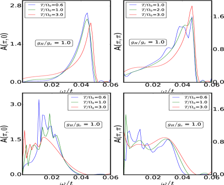
Figure 9: Lineshapes of optical (top panel) and acoustic (bottom panel) phonons at $(\pi,0)$ and $(\pi,\pi)$ for intermediate coupling ($g_{H}/g_{c}=1.0$). The relevant temperatures along with color codes are listed.

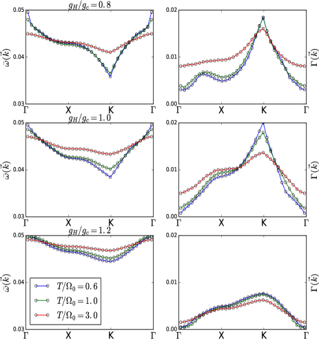
Figure 10: Fitting of optical phonon spectra at finite temperature in terms of mean frequencies ($\bar{\omega}(\vec{k})$) and linewidths ($\Gamma(\vec{k})$) throughout the BZ trajectory $(0,0)\rightarrow(\pi,0)\rightarrow(\pi,\pi)\rightarrow(0,0)$. Each panel contains three temperatures- $T/\Omega_{0}=(0.6,1.0,3.0)$. Coupling increases from top to bottom in the following sequence- $g_{H}/g_{c}=(0.8,1.0,1.2)$.

At $g_{H}=g_{c}$, polarons appear and the optical phonon spectrum becomes significantly broad due to presence of quasi-localized phonons. Except modes near the zone center ($0,0$), where scattering is prohibited owing to phase space constraints, a dramatic damping effect is seen. The softening is much less compared to the clean problem.

Beyond the polaronic transition ($g_{H}/g_{c}=1.25$), the phonon branch sharpens again and the softening is considerably less. We see a remnant of the branching feature, observed prominently for the clean problem over a region in momentum space (from $X$ to $K$), owing to charge correlations and the resulting imperfect order.

Moving to the second row, we discuss the acoustic phonon features now. Below $g_{H}=g_{c}$, the mode is clearly dispersive except around $(\pi,\pi)$, where it softens remarkably. We relate this feature, as in the case of optical phonons, to the proximity to a nesting instability ($n=0.4$ in our study). We note that acoustic phonons respond to nesting physics much more dramatically, despite disorder effects being present.

At $g_{H}=g_{c}$, polarons formation causes the phonon distribution to become significantly broad due to formation of large static distortions. Except modes near the zone center ($0,0$), where scattering is prohibited owing to the form of acoustic phonon-conduction electron coupling, a dramatic softening and damping is seen.

Beyond the polaronic transition ($g_{H}/g_{c}=1.25$), the phonon branch sharpens again and the softening is considerably reduced. States near the Fermi level are depleted in this regime and hence the scattering is less.

III.3 Detailed behaviour of phonon modes

III.3.1 Optical phonons

The optical phonon lineshapes in the ground state (top row of Fig.4) suggest that at $(\pi,0)$, we have a well-defined mode at weak coupling ($g_{H}/g_{c}=0.8$). The spectrum evolves to one having a long tail towards lower frequencies close to the crossover. But, on going further in the polaronic phase, the mode sharpens once again, with a mild, split-peak feature.

The right panel in the top row exhibits the $(\pi,\pi)$ lineshape. This is broad even at weak coupling, with more weight in lower frequencies. We ascribe this behaviour to presence of disorder and proximity to perfect nesting, as discussed earlier. On moving close to the crossover ($g_{H}/g_{c}=1.0$), the decoherence is more severe. Large static distortions are deemed responsible for this. The spectrum sharpens and hardens at strong coupling ($g_{H}/g_{c}=1.2$). There’s a hint of spectral splitting as well.

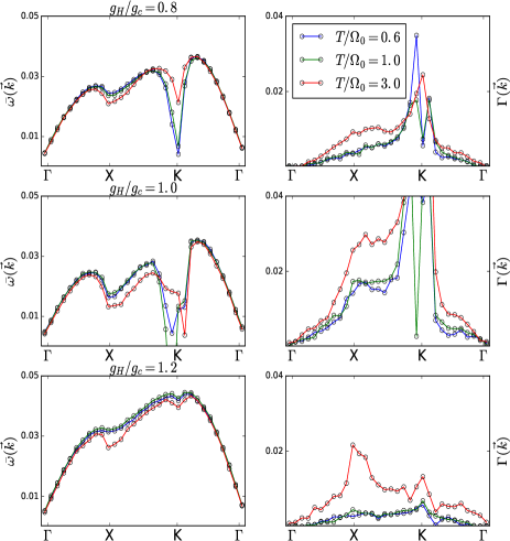
Figure 11: Fitting of acoustic phonon spectra at finite temperature in terms of mean frequencies ($\bar{\omega}(\vec{k})$) and linewidths ($\Gamma(\vec{k})$) throughout the BZ trajectory $(0,0)\rightarrow(\pi,0)\rightarrow(\pi,\pi)\rightarrow(0,0)$. Each panel contains three temperatures- $T/\Omega_{0}=(0.6,1.0,3.0)$. Coupling increases from top to bottom in the following sequence- $g_{H}/g_{c}=(0.8,1.0,1.2)$.

To gain further insight into the phonon features across the full Brillouin zone, we’ve extracted mean frequencies and linewidths along the BZ trajectory mentioned in the maps. These are provided in the top row of Fig.5. The softening (left panel) is clearly dominant at $(\pi,\pi)$, and decreases at strong coupling. The linewdiths also feature a peak at the same momentum point. The signature is most prominent at intermediate coupling, when polarons start forming but short-range correlations are still nascent.

III.3.2 Acoustic phonons

The acoustic phonon lineshapes on the ground state (bottom row of Fig.4) show qualitatively similar trends to the corresponding optical phonons at $(\pi,0)$ (left panel). One notable difference lies in the fact that the mode softens instead of hardening at intermediate coupling ($g_{H}/g_{c}=1.0$). In the deep polaronic phase, the spectrum shifts again to higher frequencies and lifetime is bandwidth limited.

The $(\pi,\pi)$ lineshapes (right panel) are more non-trivial to interpret. The weak coupling spectrum has a mode at very low ($\omega/t=0.01$) frequency. This is connected to Kohn anomaly. Additionally, a broad shoulder is observed, owing to disorder effects. The coherence at low frequency is lost out closer to the transition, where the static optical mode has large distortions. Going to higher coupling ($g_{H}/g_{c}=1.2$), the mode is still broad but regains sharp features near the bare frequency. A splitting character is observed similar to optical phonons.

In the bottom row of Fig.5, we plot the mean frequencies and widths, as in case of optical modes. The undamped Goldstone mode at $(0,0)$ is omitted for clarity. The sharp dip of mean values near $(\pi,\pi)$ is underlined (left panel). Corresponding linewidths, interpreted as lifetimes, increase markedly near the transition ($g_{H}/g_{c}=1.0$). We relate this to emerging short-range correlations amongst polarons. Once the ordering sets in at strong coupling ($g/g_{c}=1.2$), widths decrease again.

IV Effect of thermal fluctuations

After discussing phonon properties for the ground state and relating them to background and electronic features, we now move to the thermal physics. Fig.1 depicts the thermal phase diagram in our model for high ($n\sim 0.4$) denisties. The FM and PM are ferromagnetic and paramagnetic metallic phases. The corresponding insulating phases are FI and PI, respectively. The blue-lettered regions are phonon regimes. In the weak coupling regime, standard perturbation theory results for phonons are useful. In the fan-like crossover region, phonons are very broad ($\Gamma\sim\Omega_{0}$). Towards the right, we have narrow band optical phonons. Compared to the clean Holstein phase diagramsauri , we see the region featuring electronic pseudogap and ‘crossover’ phonons have shifted to the left. The electronic phases are indicated in black letters.

IV.1 Backgrounds

The ground state of our model is ferromagnetically ordered at all coupling windows, owing to double exchange interaction. We first plot the $S(0,0)$ structure factor to infer $T_{c}$ scales (top left panel of Fig. 6). At weak coupling $g_{H}/g_{c}=0.8$, the $T_{c}\sim 0.07t$. This value reduces to $T_{c}\sim 0.04t$ at strong coupling ($g/g_{c}=1.2$). The ferromangetic $T_{c}$ plays an important role in the broadening of phonons as the interplay of spin disorder and thermal fluctuations has direct impact on the electronic spectrum. This in turn feeds back to the phonons through the polarization $\Pi_{ij}(\omega)$ within our calculation.

The top right and bottom (left and right) panels of Fig.6 show static phonon structure factors (shown for the ground state in Fig.2, middle panel) at finite temperature. The rising feature near ($\pi,\pi$) survives and in fact grows mildly on heating at weak coupling.

In Fig.7, the first row depicts static distributions of optical mode distortions in various coupling regimes. The left panel features weak coupling regime, where the hint of bimodality observed in the ground state is wiped out on mild heating. Increasing the temperature further (going beyond ferro $T_{c}\sim 0.07t$), we see a very broad distribution skewed to lower $x$ values. The intermediate coupling (middle panel) picture retains bimodality upto the bare phonon scale $T/\Omega_{0}=1.0$. At strong coupling, even at high $T$, we have a two-peak feature.

In the bottom row (Fig.7), thermal dependence of electronic DoS is shown. The most non-trivial feature is a weak hint of pseudogap at weak coupling (left panel). This arises out of spin disorder, causing effective electron hopping to weaken. There are also large thermal fluctuations of the static mode, which grow into actual distortions at intermediate coupling ($g_{H}/g_{c}=1.0$). There’s a pseudogap surviving upto high temperature in the middle panel (close to crossover). At higher coupling (right panel), the lowest $T$ features a small gap, that develops into a robust pseudogap on heating up.

IV.2 Overview of phonon modes

Optical phonons

In Fig.8 (left set), we observe the spectral maps of the optical (left) and acoustic (right) phonons in various coupling and temperature regimes. The first row is representative of phonons at low $T$ ($T/\Omega_{0}=0.6$). Ferromagnetic order is still present in the background. Below $g_{H}=g_{c}$, the mode is still ‘dispersive’ except around $(\pi,\pi)$, where the softening feature is retained. At $g_{H}=g_{c}$, we now have thermal fluctuations of large static distortions playing out in tandem with magnetic fluctuations. Except modes near the zone center ($0,0$), a dramatic softening and damping is seen. The high temperature phonons are very broad ($\Gamma\sim\Omega$). Beyond the polaronic transition ($g_{H}/g_{c}=1.25$), the phonon branch sharpens again and the softening is considerably reduced. The mild branching feature observed near ($\pi,\pi$) for the ground state is washed out. The role of disorder is to effectively promote electronic spectral gaps. Consequently, these phonons are less broad compared to those in the clean Holstein model.

Acoustic phonons

Moving to the spectral maps of the finite temperature acoustic phonons (Fig.8, right set), at the scale of bare Holstein frequency ($T/\Omega_{0}=1.0$), we observe quantitative changes at weak and strong coupling but a significant increase in lifetimes for the middle (intermediate coupling) picture. At even higher temperatures, well past the ferro $T_{c}$ scale for all couplings, phonons in the polaronic side are rendered quite broad and incoherent, except at low wavevectors. The metallic side ($g_{H}/g_{c}\sim 0.8$) is affected mostly near $(\pi,\pi)$, where the degree of softening reduces and lifetime picks up.

IV.3 Detailed behaviour of phonon modes

As in case of the ground state, we study the phonons more closely by examining specific lineshapes and fitting the full spectrum to find mean frequencies and linewidths. Here, we focus on the most interesting regime of intermediate coupling ($g_{H}/g_{c}=1.0$).

Optical phonons

In this regime, the polaronic crossover causes both the ($\pi,0$) and ($\pi,\pi$) lineshapes to have long tails at all temperature windows, as seen in Fig.9 (top panel). The effect of large static distortions is most prominent in the ($\pi,\pi$) lineshapes. Some features of sharp peaks remain at low $T$, owing to limited system size ($24\times 24$) which gradually smudge out, giving an incoherent spectrum with some weight near the unrenormalized frequency on further heating ($T/\Omega_{0}=3.0$). One may ascribe this behaviour partly to loss of ferromagnetic order also, which takes place around $T=0.06t$.

Fig.10 shows the mean frequencies (left column) and linewidths (right column) as functions of temperature for three regimes. The trends mentioned previously are clealy visible. First, at ‘weak’ coupling, proximity to a nesting instability creates phonon softening around the zone boundary. broadenings also pick up in that region. On heating up across the ferromagnetic $T_{c}\sim 0.07t$, a marked increase in lifetimes take place. The momentum dependence of the spectrum is also subdued. Moving to the polaronic crossover regime, the ground state picture is roughly unaltered, whereas thermal broadenings generally decrease, due to formation of short-range correlations. This effect is markedly observed moving to the strong coupling (third column) plots. The mean (or mode) frequencies harden and lifetimes become limited by the bandwidth, which scales as $\frac{t^{2}}{E_{p}}$.

Acoustic phonons

At intermediate coupling, the polaronic crossover imparts an overall damping of acoustic phonon spectrum throughout the Brillouin Zone (BZ). However, the effect is most drastic around $(\pi,\pi)$, where across a wide range of temperatures, a ‘box-like’ lineshape emerges (Fig.10, bottom panel). The thermal dependence of lineshapes is not very significant. Even at $(\pi,0)$, there are large lifetimes present along with prominent softening, especially at high T ($T/\Omega_{0}=3.0$).

The corresponding fitting plots of the acoustic phonons are exhibited in Fig.11. The left column, depicting the mean frequencies, show prominent dips at both $(0,0)$ and $(\pi,\pi)$ in the weak coupling regime. The Goldstone mode at $\Gamma$ point is undamped (not shown explicitly). The softening of phonon mode at $(\pi,\pi)$ owes its origin to Kohn anomaly. Close to the crossover, broadenings increase quantitatively, due to formation of large static distortions and consequent phonon localization. Thermal fluctuations magnify the effect remarakably past the ferromagnetic $T_{c}\sim 0.06t$. Low momentum modes are protected from scattering because of phase space restrictions. At strong coupling, the dispersion regains clarity to a large degree. Only on heating up to $T/\Omega_{0}=3.0$, one observes significant broadenings, near $(\pi,0)$.

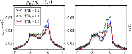
Figure 12: Fitting of acoustic phonon spectra at finite temperature in terms of ‘softenings’ (deviation of mean frequencies ($\bar{\omega}(\vec{k})$ form bare values) and linewidths ($\Gamma(\vec{k})$ through the BZ trajectory $(0,0)\rightarrow(\pi,\pi)$. The coupling is $g_{H}/g_{c}=1.0$. Temperature increases in the following sequence- $T/\Omega_{0}=(1.2,1.4,1.6)$. The ferromagnetic transition occurs at $T_{c}=1.2\Omega_{0}$

.

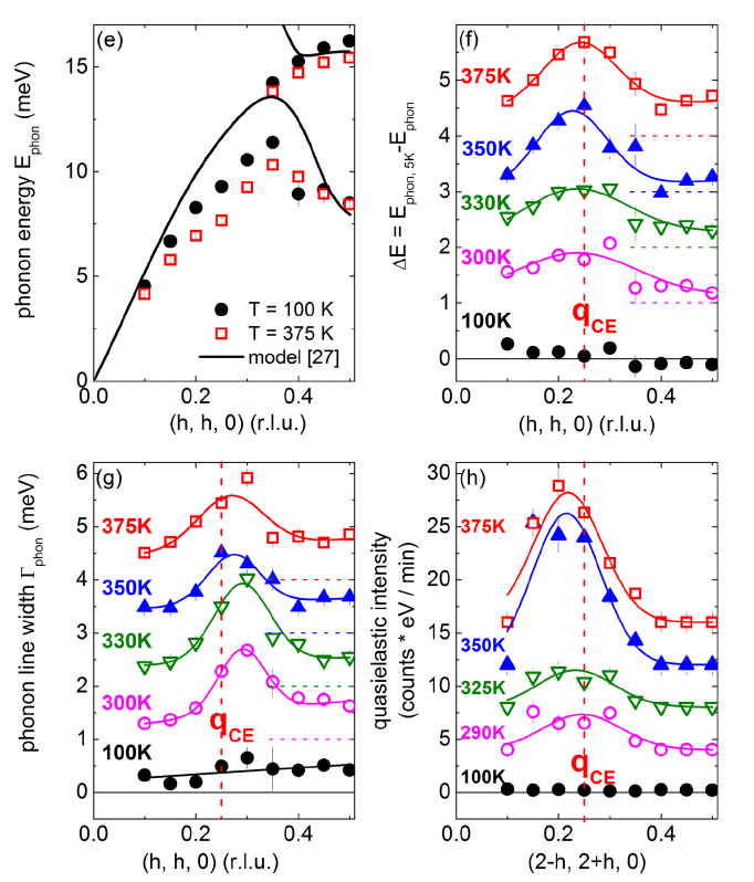
Figure 13: Summary of investigations on transverse acoustic phonons in La_0.7Sr_0.3MnO₃. In panel (e) (top left), we have phonon energies in meV at two different temperatures ($100K$ and $375K$). Also, a model calculation is shown. In panel (f) (top right), phonon softenings compared to low$T$ ($5K$) values are featured for several temperatures along the $(hh0)$ direction in BZ. The $T_{c}=350K$ marks the onset of pronounced softenings around $\vec{q}_{CE}$. The bottom left panel (g) shows corresponding linewidths, which pick up just before the metal-metal transition. Lastly, in panel (h) (bottom right), one has quasi-elastic intensitites quantifying short-range ordering of polarons beyond $T_{c}$.

V Discussion

We list below the salient features of the phonon modes revealed through our investigation-

• The low temperature state of our model is ferromagnetically ordered and shows charge correlations at strong coupling.

• The weak coupling ‘disordered metal’ at low $T$ is in proximity to a nesting instability for $n\sim 0.5$. As a result, both optical and acoustic modes are softened considerably around $(\pi,\pi)$.

• On heating up the weak coupling state, two effects occur simultaneously. Firstly, thermal fluctuations induce large static distortions in the optical mode. Secondly, the ferromagnetic order is lost as one goes across $T_{c}\sim 0.1t$. This leads to broad, flat optical phonon spectrum and a loss of coherence (barring small wavevectors) in the acoustic mode. These features are correlated with the appearance of a weak pseudogap in the electronic density of states, owing to spin disorder.

• The intermediate coupling state is on the verge of a polaronic transition. So, phonon eigenstates tend to get localized. This results in generally broad phonon modes except around $(0,0)$. On increasing temperature, the lifetimes increase quantitatively, along with a flattening of the optical phonons. The electronic spectrum is already pseudogapped in the ground state, the extent of which becomes milder on heating up.

• At stronger couplings, a short-range $(\pi,\pi)$ order sets in amongst polarons at low $T$. As a result, the electronic spectrum shows a small hard gap. There’s a depletion of states near Fermi level, leading to weaker low-energy weights in the polarization based self-energy for the phonons. Consequently, both acoustic and optical modes regain some coherence. The damping is bandwidth limited $\Gamma\sim\frac{t^{2}}{E_{p}}$.

• Heating up and going across the ferro $T_{c}$ (which is almost half of its weak-coupling value), one creates a more disordered background for the phonons to propagate. This causes broadening effects to pick up. The electronic spectrum shows a prominent pseudogap and the acoustic phonons are broadened considerably.

We’ve tried out a qualitative comparison with actual experimental data for acoustic phonons in La_0.7Sr_0.3MnO₃weber2 . Fig. 12 summarizes our results. The general trends show an agreement. Our acoustic phonons show increased softening and broadening effects at intermediate coupling ($g_{H}/g_{c}=1.0$) just before the ferromagnetic transition $T_{c}\sim 1.2\Omega$ at $K$ point. This is also the important wavevector for short-range ordering of polarons. Correspondingly, in the experimental plots (Fig. 13), we see around $\vec{q}_{CE}$, the softening and linewidths pick up, just before $T_{c}=350K$. The increase is monotonic in both cases along the BZ trajectories chosen. The quasielastic intensity, which quantifies short-range ordering of distortions, shows a marked increase near the same wavevector at $T_{c}$. On crossing this temperature, both the theoretical and experimental curves show a mild reduction in broadenings.

VI Conclusions

In conclusion, we’ve studied the phonon spectrum of the weakly disordered double exchange Holstein model in two dimensions. The results have direct implications for recent inelastic neutron scattering experiments in manganites. The novelty of the method is to be able to capture short-range correlations amongst polarons and resulting pseudogap features in the electronic spectrum at finite temperature. This in turn affects the polarization of the system, which renormalize the acoustic and optical phonons. The most interesting region in our parameter space is one of intermediate coupling and temperature, when polarons start forming and the ferromagnetic order in the ground state is on the verge of destruction. We’ve quantified the observed spectrum through detailed fitting across BZ and an analysis of lineshapes at specific high-symmetry points. We are investigating the problem at even weaker values of binary disorder, so as to disentangle the polaron physics from the effect of disorder. We also wish to compare our findings with experiments in more detail in the future.

Acknowledgement: We acknowledge the use of HPC clusters at HRI. SB acknowledges fruitful discussions with Samrat Kadge and Abhishek Joshi, and thanks Samrat Kadge for a careful reading of the manuscript. The research of SB was partly supported by an Infosys scholarship for senior students. The research of SP was partly supported by the Olle Engkvist Byggmästare Foundation.

References

- [1] P. Bruesch, Phonons: Theory and Experiments, Vols. I-III, Springer (1982).
- [2] E. Dagotto, Science 309, 257 (2005).
- [3] Y. Tokura, Colossal Magnetoresistive Oxides, CRC Press (2000).
- [4] Handbook on the Physics and Chemistry of Rare Earths, edited by K.A.Jr. Gschneidner, L. Eyring, M.B. Maple, North Holland (2000), Vols.30-31.
- [5] F. Weber, N. Aliouane, H. Zheng, J.F. Mitchell, D.N. Argyriou, and D.Reznik, Nature Materials 8, 798 (2009).
- [6] M. Maschek, D. Lamago, J.-P. Castellan, A. Bosak, D. Reznik, and F. Weber, Phys. Rev. B 93, 045112 (2016)
- [7] F. Weber, S. Rosenkranz, J.-P. Castellan, R. Osborn, H. Zheng, J.F. Mitchell, Y. Chen, Songxue Chi, J. W. Lynn, and D. Reznik, Phys. Rev. Lett. 107, 207202 (2011).
- [8] D. Reznik Advances in Condensed Matter Physics, Vol. 2010, Article ID 523549 (2010).
- [9] H. Miao, D. Ishikawa, R.Heid, M. Le Tacon, G. Fabbris, D. Meyers, G.D. Gu, A.Q.R. Baron and M.P.M. Dean, arXiv 1712.04554.
- [10] R. Kajimoto, M. Fujita, K. Nakajima, K. Ikeuchi, Y. Inamura, M. Nakamura and T. Imasoto, Journal of Physics, Conference Series 502 012056 (2014).
- [11] M. Braden, W. Reichardt, S. Shiryaev and S.N. Barilo, Physica C 378-381 (2002) 89-96.
- [12] A.J. Millis, P.B. Littlewood and B.I. Shraiman, Phys. Rev. Lett. 74, 5144 (1995).
- [13] R. Blankenbecler, D.J. Scalapino, and R.L. Sugar, Phys. Rev. D 24, 8 (1981).
- [14] A. Georges, G. Koliar, W. Krauth, and M.J. Rozenberg, Rev. Mod. Phys. 68, 13 (1996).
- [15] Stefan Blawid, Andreas Deppeler, and A.J. Millis, Phys. Rev. B 67, 165105 (2003).
- [16] Sauri Bhattacharyya, Saurabh Pradhan and Pinaki Majumdar, arXiv 1711.08749 (2017).