VEBO: A Vertex- and Edge-Balanced Ordering Heuristic to Load Balance Parallel Graph Processing

Abstract

Graph partitioning drives graph processing in distributed, disk-based and NUMA-aware systems. A commonly used partitioning goal is to balance the number of edges per partition in conjunction with minimizing the edge or vertex cut. While this type of partitioning is computationally expensive, we observe that such topology-driven partitioning nonetheless results in computational load imbalance.

We propose Vertex- and Edge-Balanced Ordering (VEBO): balance the number of edges and the number of unique destinations of those edges. VEBO optimally balances edges and vertices for graphs with a power-law degree distribution. Experimental evaluation on three shared-memory graph processing systems (Ligra, Polymer and GraphGrind) shows that VEBO achieves excellent load balance and improves performance by 1.09x over Ligra, 1.41x over Polymer and 1.65x over GraphGrind, compared to their respective partitioning algorithms, averaged across 8 algorithms and 7 graphs.

I Introduction

Graph partitioning is used extensively to orchestrate parallel execution of graph processing in distributed systems [1], disk-based processing [2, 3] and NUMA-aware shared memory systems [4, 5]. In order to maximize processing speed, each partition should take the same amount of processing time. Moreover, the partitions should be largely independent to minimize the volume of data communication. It has been demonstrated that partitioning the edge set is more effective than partitioning the vertex set [1], leading to the commonly used heuristic to balance edge counts and minimize vertex replication [1, 6, 7, 2]. These constraints are typically mutually incompatible for scale-free graphs, resulting in a compromise between edge balance and vertex replication [6].

We have observed, however, that edge balance does not uniquely determine execution time. For instance, for an approximating PageRankDelta [8] computation, during a first phase of the algorithm, about half of low-degree vertices converge before any high-degree vertex converges. A partition that consists of mostly high-degree vertices will thus take longer to process than a partition with only low-degree vertices, resulting in load imbalance. Note that it is likely to encounter partitions with mostly low-degree vertices in graphs with a power-law degree distribution as these graphs have many more low-degree vertices than high-degree vertices.

The key contribution of this paper is to identify that the time for processing a graph partition depends on both the number of edges and the number of unique destinations in that partition. This presents a new heuristic to partition graphs through joint destination vertex- and edge-balanced partitioning, which we call VEBO.

A key motivation for considering joint vertex and edge balancing is provided by the classification of Sun et al, who observed a distinction between edge-oriented algorithms and vertex-oriented algorithms [5]. Edge-oriented algorithms, like PageRank, perform an amount of computation proportional to the number of edges. In contrast, vertex-oriented algorithms, like Breadth-First Search, perform an amount of computation proportional to the number of vertices. These properties strongly affect partitioning: a vertex-balanced partition can result in almost a 40% speedup compared to edge-balanced partitioning for vertex-oriented algorithms [5]. While Sun et al selected the partitioning heuristic depending on the algorithm, VEBO seamlessly resolves this important distinction between algorithm types.

A second important contribution of this work is to identify a need to adapt vertex order to the characteristics of the graph processing system. Each system has unique design choices, which determine its key performance bottlenecks. For instance, Ligra [8] uses dynamic scheduling to manage parallelism, but does itself not improve memory locality. In contrast, Polymer [4] and GraphGrind [5] perform NUMA-aware data layout and use static scheduling in order to bind computation to the appropriate NUMA domains. Static scheduling makes parallel loops sensitive to load balance as the execution time of the loop is determined by the last-completing thread. It may thus be expected that vertex ordering serves different purposes: for Ligra, memory locality should be improved, while for Polymer and GraphGrind, load balance is more important.

We propose a graph partitioning algorithm that calculates an optimally load-balanced partition for power-law graphs with time complexity $\mathcal{O}(n\log P)$, where $n$ is the number of vertices in the graph and $P$ is the number of partitions. Extensive experimental evaluation using three shared memory graph processing systems demonstrates a near-perfect computational load balance across a variety of graph data sets and algorithms. Contrary to heuristics such as Reverse Cuthill-McKee (RCM) [9] and Gorder [10] that aim to optimize memory locality, we obtain a consistent performance improvement when processing seven scale-free graphs.

In summary, this paper makes the following contributions:

1. Demonstrating the need to balance the number of unique destinations along with the number of edges in order to achieve computational load balance

2. A simple vertex reordering algorithm that optimally balances both edges and unique destinations using time proportional to $\mathcal{O}(n\log P)$

3. Addressing vertex-oriented and edge-oriented algorithms using a single graph partitioning heuristic

4. Extensive experimental evaluation using three shared memory graph processing systems (Ligra, Polymer and GraphGrind) and a comparison to edge balancing

The remainder of this paper is organized as follows: Section II motivates the load balancing heuristic. Section III presents the VEBO algorithm and proves its optimality. Section IV presents our experimental evaluation methodology. The experimental evaluation of VEBO is presented in Section V. Related work is discussed in Section VI.

input : Graph $G=(V,E)$; number of partitions $P$

output : Graph partitions $G_{i}=(V,E[i])$ for $i=0,\ldots,P-1$

1

Let avg = $|E|/P$;

  // target edges per partition

Let E[P] = { 0 };

  // array of length $P$, initialized to 0

2 Let i = 0;

3 for $t\leftarrow 0$ to $|V|-1$ do

       Let $v=v_{t}$;

        // the $t$-th vertex

4       if $|E[i]|$ $\geq$ avg and i $<P-1$ then

             ++i;

              // E[i] has exceeded target edges

5            

       E[i] = E[i] $\ \cup$ in-edges($v$);

        // i is home partition of v

6      

7

ALGORITHM 1 Locality-preserving edge-balanced partitioning of the destination vertices

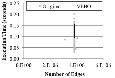
(a) Twitter

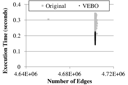
(b) Friendster

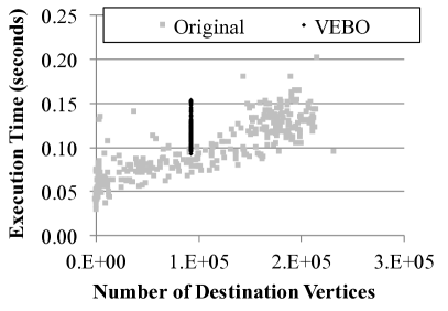
(c) Twitter

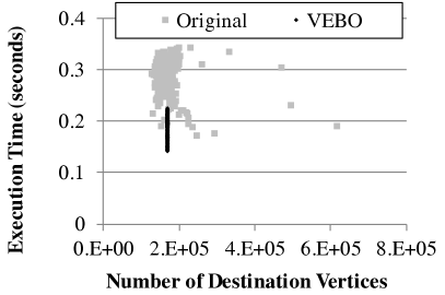
(d) Friendster

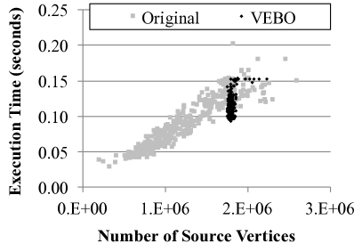
(e) Twitter

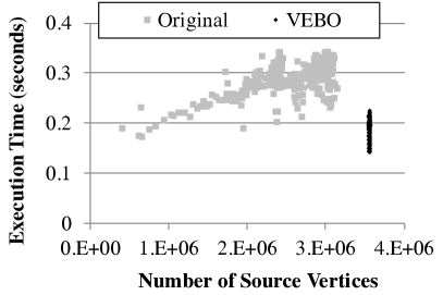
(f) Friendster

Figure 1: Processing time of a partition as a function of the number of edges, destinations, and source vertices in the partition. Each data point corresponds to one of 384 partitions. Average time of Twitter in original is 0.119s and in VEBO is 0.111s. Average time of Friendster in original is 0.289s and in VEBO is 0.234s.

II Motivation

The edge-balance heuristic is commonly used to balance the computation. Algorithm 1 shows a simple, locality-preserving edge balancing algorithm for graph partitioning. We call it partitioning by destination as edges are assigned to the partition that holds their destination vertex. The algorithm is locality-preserving in the sense that each partition consists of a chunk of consecutively numbered vertices. This algorithm is used in disk-based [2] and NUMA-aware graph processing [4, 5].

Figure 1 shows the processing time for each of 384 partitions when executing one iteration of the PageRank algorithm. The graph is represented using the coordinate format (COO) and edges are sorted in the access order of a Hilbert space filling curve in order to improve memory locality [11, 12]. Each partition is processed sequentially by one thread. We study the Twitter and Friendster graphs. Details on the graphs and experimental setup are provided in Section IV.

The top two plots in Figure 1 show that Algorithm 1 achieves good edge balance. There is some variation on the number of edges in each partition, which results from high-degree vertices that appear at the boundary between two partitions. Placing a high-degree vertex in a first partition will overload it, placing it in the next partition will leave the first underloaded. While partitions are edge-balanced well, the execution time per partition varies over a factor of 6.9x and 2x for the Twitter and Friendster graphs, respectively. The VEBO heuristic, which we will present in the next Section, reduces to variation to 1.6x (Twitter) and 1.4x (Friendster).

The plots moreover show that the processing time of a partition is correlated to the number of destination vertices (middle row), and of source vertices (bottom). Partitions with few destination vertices (and thus holding vertices with a high in-degree) are processed faster than a partition holding many low-degree vertices.

While both the number of unique source and destination vertices in a partition affects processing time, we choose to balance the number of destinations. Balancing both source and destination numbers would be as computationally complex as minimizing edge cut and it is our express goal to minimize the time taken for partitioning. A number of graph processing systems partition the destination set to create parallelism and avoid data races [2, 4, 5]. Partitioning by destination ensures data race freedom as graph algorithms typically update values associated to the destinations of edges. Others partition the source vertices [3]. For these systems, the analogous balancing criteria would focus on the source vertices.

III The VEBO Algorithm

III-A Problem Statement

Assume a graph $G=(V,E)$ with power-law in-degree distribution. Let $N$ be one more than the highest in-degree in the graph. Let $n$ be the number of vertices and let $m$ be the number of vertices with non-zero in-degree.

We model the in-degree distribution using a Zipf distribution where $s\geq 0$ is the real-valued exponent governing the skewedness of the degree distribution, $N$ is the number of ranks and $p_{k}$, $k=1,\ldots,N$ is the probability that a vertex has degree $k-1$:

$$p_{k}=\frac{k^{-s}}{H_{N,s}}$$ (1)

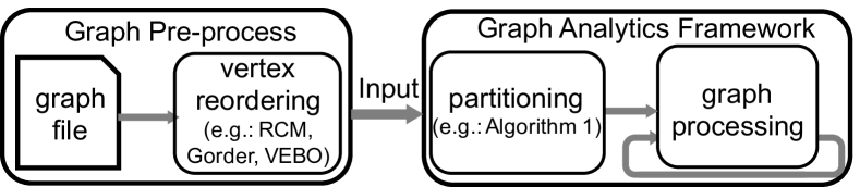
Figure 2: A graph processing pipeline with vertex reordering and graph partitioning

where $H_{N,s}=\sum_{i=1}^{N}i^{-s}$ is a Generalized Harmonic Number. As such, the most frequent in-degree in the graph is zero, and least frequent in-degree is $N-1$. We make no assumptions about the out-degree distribution.

VEBO partitions the vertex set in $P$ parts such that $V=\cup_{i=0}^{P-1}V_{i}$ and $V_{i}\cap V_{j}=\{\}$ if $i\neq j$. The partitions of the vertex set induce a partitioning of the edge set $E=\cup_{i=0}^{P-1}E_{i}$ such that for each $(v,w)\in E$: $(v,w)\in E_{i}$ if $w\in V_{i}$. The graph partitions are $G_{i}=(V,E_{i})$, where any vertex can appear as a source vertex (hence the vertex set is $V$) but the set of destinations is restricted to $V_{i}$. The VEBO optimization criteria are:

• minimize $max_{i=0}^{P-1}|E_{i}|-min_{i=0}^{P-1}|E_{i}|$ (edge balance)

• minimize $max_{i=0}^{P-1}|V_{i}|-min_{i=0}^{P-1}|V_{i}|$ (vertex balance).

These criteria address the worst-case spread of load per partition. Alternatively, criteria based on variation could be formulated which could potentially assess load imbalance with more precision. However, we will demonstrate that the worst-case spread of load is limited to 1 edge and 1 vertex. As such, these criteria are appropriate.

input : Graph $G=(V,E)$; number of partitions $P$

output : Reordered sequence numbers $S[v]\in 0,\ldots,|V|-1$ for $v\in V$ and partition end points $u[p]\in 0,\ldots,|V|-1$ for $p\in 0,\ldots,P-1$

1

Let w[P] = { 0 };

  // tracking edge count in each partition

Let u[P] = { 0 };

  // tracking vertex count in each partition

Let a[V] = { 0 };

  // assigned partition for each vertex

2 Consider the list $v_{(0)},v_{(1)},\ldots,v_{(n)}$ of vertices sorted by decreasing in-degree, i.e., $\{v_{(0)},v_{(1)},\ldots,v_{(n)}\}=V$ and $deg_{in}(v_{(i)})\geq deg_{in}(v_{(j)})$ when $i>j$;

Let n = $|V|$;

  // the number of vertices

Let m = $|\{v\in V:deg_{in}(v)>0\}|$;

  // the number of vertices

;

  // with non-zero degree

3

// Phase 1. Assign vertices with non-zero degree

4 for $t\leftarrow 0$ to $m-1$ do

5       Let $v=v_{(t)}$;

6       Let $p=\operatorname*{arg\,min}_{i=0,\ldots,P-1}w[i]$;

       Let $a[v]=p$;

        // assign $v$ to partition $p$

       Increase $w[p]$ by $deg_{in}(v)$;

        // update edge count

       Increase $u[p]$ by 1;

        // update vertex count

7      

8

9

// Phase 2. Assign vertices with zero degree

10 for $t\leftarrow m$ to $n-1$ do

11       Let $v=v_{(t)}$;

12       Let $p=\operatorname*{arg\,min}_{i=0,\ldots,P-1}u[i]$;

       Let $a[v]=p$;

        // assign $v$ to partition $p$

       Increase $u[p]$ by 1;

        // update vertex count

13      

14

// Phase 3. Calculate new sequence numbers

15 Let $s[0]=0$;

16 for $p\leftarrow 1$ to $P-1$ do

17       Let $s[p]=s[p-1]+u[p-1]$;

18      

19

20for $t\leftarrow 0$ to $n-1$ do

21       Let $v=v_{(t)}$;

       Let $S[v]=s[a[v]]$;

        // determine sequence number for $v$

22       Increment $s[a[v]]$ by 1;

23      

24

ALGORITHM 2 The VEBO reordering algorithm

III-B Algorithm Description

The core idea behind VEBO is to perform vertex reordering: each vertex is assigned a new sequence number in the range $0,\cdots,n-1$ in a way that enables Algorithm 1 to generate optimal load balance. As such, vertex reordering precedes partitioning (Figure 2). We follow an approach similar to the multi-processor job scheduling heuristic [13]: place a set of objects in order of decreasing size, for each object selecting the least-loaded partition. In our case, however, we adapt the algorithm to balance both the number of objects (vertices) and their size (degree).

The VEBO algorithm (Algorithm 2) consists of three phases: In the first phase, VEBO places vertices with non-zero in-degree in order of decreasing in-degree. This achieves a near-equal edge count in each partition. We will show that edge imbalance is just 1 edge when the size of the placed objects follows a power-law distribution. In the second phase, zero-degree vertices are placed. We observe that real-world graphs may have many zero-degree vertices. These vertices do not affect edge balance. If any vertex imbalance is introduced during the first phase, the vertex imbalance is corrected by placement of the zero-degree vertices. The third phase reorders the vertices. It assigns new sequence numbers to the vertices such that each partition consists of a continuous sequence of vertices. This is important to retain spatial locality and NUMA locality during graph processing [2, 4, 12].

III-C Example

Figure 3 shows a short example. VEBO first sorts the vertices by decreasing in-degree. Second, it assigns vertices one by one to the partition that has the fewest incoming edges among all of the vertices already assigned to it. When all vertices have been placed, the vertices are assigned new IDs such that each partition spans a range of consecutive vertex IDs. This actual reordering is beneficial for spatial locality. Finally, a new graph representation is generated using the new vertex IDs. Figure 3b) shows how the graph is partitioned. Each partition has 7 incoming edges and 3 destination vertices.

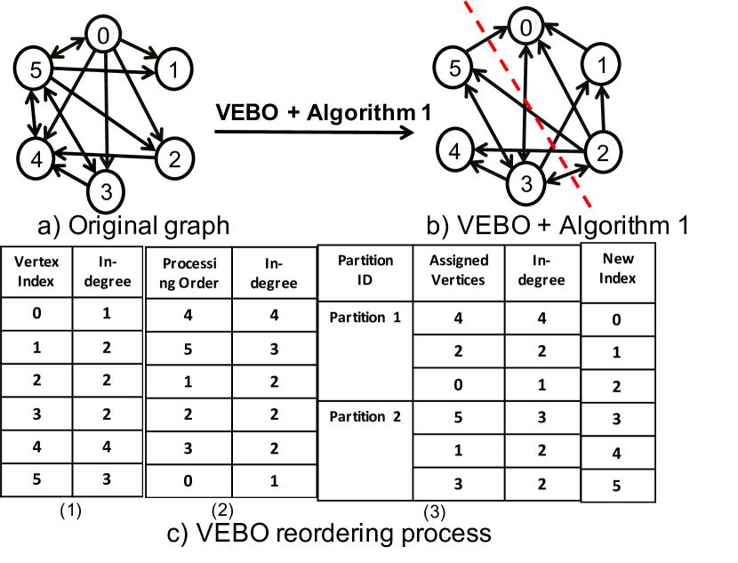
Figure 3: Illustration of VEBO on a 6-vertex graph

III-D Analysis

To support analysis of the algorithm, we introduce some auxiliary definitions. Let $v_{(0)},v_{(1)},\ldots,v_{(n-1)}$ be the sequence that holds all vertices in $V$ in order of decreasing degree. Assume the algorithm goes through $n=|V|$ steps to place the vertices. Step $t>0$ corresponds to placing vertex $v_{(t)}$. The algorithm terminates when $t=|V|$.

Let $w_{p}(t)$ be the number of edges assigned to partition $p$ before step $t$, i.e., before placing vertex $v_{(t)}$. The initial situation is $w_{p}(0)=0$ for all $p$. The maximum weight before step $t$ is: $\omega(t)=\max_{j=1,\ldots,P}w_{j}(t)$ The minimum weight before step $t$ is: $\mu(t)=\min_{j=1,\ldots,P}w_{j}(t)$ The edge imbalance before step $t$ is: $\Delta(t)=\omega(t)-\mu(t)$ An optimal edge placement is achieved when $\Delta(n)\leq 1$, i.e., the number of edges in each partition differs by at most 1. $\Delta(n)=0$ can occur only when the number of partitions divides into the number of edges. The vertex imbalance before step $t$ is: $\delta(t)=\max_{j=1,\ldots,P}u_{j}(t)-\min_{j=1,\ldots,P}u_{j}(t)$ where $u_{p}(t)$ is the number of vertices assigned to partition $p$ before step $t$.

We first prove the following Lemma that bounds the edge imbalance throughout the placement of vertices. As a short-hand, let $d_{(t)}=deg_{in}(v_{(t)})$ for $t=0,\ldots,n-1$. Clearly, $d_{(i)}\geq d_{(j)}$ if $i<j$ and $d_{(0)}=N-1$.

Lemma 1.

When placing a vertex $v_{(t)}$ with degree $d_{(t)}$ when the edge weight is $w_{j}(t)$ for $j\in 1,\ldots,P$, one of following cases can occur:

$$\left.\begin{array}[]{ll}\Delta(t+1)\leq\Delta(t)\\ \omega(t+1)=\omega(t)\end{array}\right\} d_{(t)}\leq\Delta(t)$$ if (4)

$$\left.\begin{array}[]{ll}\Delta(t+1)\leq d_{(t)}\\ \omega(t+1)>\omega(t)\end{array}\right\} d_{(t)}>\Delta(t)$$ if (7)

Proof.

We sketch the proof for brevity. Vertex $v_{(t)}$ is placed on the partition $p$ with minimal $w_{p}(t)$, i.e., $w_{p}(t)=\mu(t)$. The edge count of $p$ increases to $\mu(t)+d_{(t)}$. Two cases arise depending on whether the maximum load on a parition is raised ($\mu(t)+d_{(t)}>\omega(t)$ and thus $d_{(t)}>\Delta(t)$) or not ($d_{(t)}\leq\Delta(t)$). The Lemma follows by elaboration of the definitions of $\Delta(t)$ and $\omega(t)$. ∎

Intuitively, by placing more edges we either strive towards balancing the edge counts (case 4), or we are so close to load balance that placing the next vertex must increase the load imbalance (case 7). Importantly, in the latter case, the load imbalance is bounded by the degree of the last vertex placed. As we process vertices in order of decreasing degree, the edge imbalance reduces throughout the algorithm.

Theorem 1 (Edge balance).

Assume a graph $G=(V,E)$ and a number of partitions $P$. Let $n=|V|$ be the number of vertices and let $m$ be the number of vertices with non-zero degree. Assume that the degree distribution of the graph follows a Zipf distribution with $N$ distinct ranks and scale factor $s>0$. Let $|E|$ be the number of edges. Assume that $P$ is constrained by $|E|\geq N\>(P-1)$ and that $P<N$. Then, on completion of VEBO (Algorithm 2),

$$\Delta(n)\leq 1$$ (8)

Proof.

We sketch the proof. It builds on the observation that the final edge imbalance $\Delta(n)$ is at most 1 if the maximum weight $\omega(t)$ can be increased by placing a degree-1 vertex (Lemma 1, Eq 7). Degree-1 vertices are abundant under the assumption of the Zipf distribution. As such, one can show that at any step $t$ where $d_{(t)}>\Delta(t)$, there are at least $(P-1)\Delta(t)$ edges among the unplaced vertices, i.e., $\sum_{i=t^{{}^{\prime}}}^{m-1}d_{(i)}\geq(P-1)\Delta(t)$. This relation follows from the assumption $|E|\geq P(N-1)$ and the recurrence $\sum_{i=1}^{N_{1}}(i-1)\>i^{-s}/N_{1}\geq\sum_{i=1}^{N}(i-1)\>i^{-s}/N$ if $N_{1}<N$. ∎

The condition $|E|\geq N(P-1)$ can be understood as follows: As the highest degree is $N-1$, and all edges pointing to this vertex are placed in the same partition, at least one partition will have $N-1$ edges. In order to have edge balance, the other $P-1$ partitions may have at most $N$ edges. As such, $|E|\geq(N-1)+(P-1)(N-2)=P(N-2)+1$ is a necessary condition for edge balance. The theorem makes only a slightly stronger requirement.

Theorem 2 (Vertex balance).

Assume a graph $G=(V,E)$ and a number of partitions $P$ as required for Theorem 1. Assume that $n\geq N\>H_{N,s}$. Under these conditions, upon placement of vertices $v_{(0)},v_{(1)},\ldots,v_{(m-1)}$ by Algorithm 2, it holds that $\delta(m)<N/P$ and upon placement of all vertices by Algorithm 2, it holds that $\delta(n)\leq 1$.

Proof.

The proof first shows that the vertex imbalance is bound as $\delta(m)<N/P$ after placing vertices with non-zero degree. Then, vertex balance can be achieved if at least $\delta(m)\>(P-1)$ zero-degree vertices are available, which follows from the properties of the degree distribution. ∎

The condition $n\geq N\>H_{N,s}$ in Theorem 2 dictates that there should be a sufficiently large number of vertices in the graph. The number of vertices is independent of the parameters $N$ and $s$ which determine the shape of the degree distribution. This constraint is not stringent, e.g., if $s=1$, then the requirement is $n\geq 2\>N$.

TABLE I: Characterization of real-world and synthetic graphs used in experiments.

			Max.	% vertices with	% vertices with
Graph	Vertices	Edges	Degree	zero in-degree	zero out-degree	$\delta(n)$	$\Delta(n)$	Type
Twitter [14]	41.7M	1.467B	770,155	14%	4%	1	1	directed
Friendster [15]	125M	1.81B	4,223	48%	37%	1	1	directed
Orkut [15]	3.07M	234M	33,313	0%(186)	0%(186)	2	1	undirected
LiveJournal [15]	4.85M	69.0M	13,906	7%	21%	1	1	directed
Yahoo_mem [15]	1.64M	30.4M	5,429	0%(0)	0%(0)	9	3	undirected
USAroad [4]	23.9M	58M	9	0%(1)	0%(1)	1	1	undirected
Powerlaw ($\alpha=2$)	100M	294M	132,423	0%(99)	0%(99)	1	1	undirected
RMAT27 [8]	134M	1.342B	812,983	69%	69%	1	1	directed

VEBO is applied to 8 graphs with a selection of synthetic and real-world graphs (Table I). Seven graphs are power-law graphs. The USARoad graph represents a road network and has nearly constant degree. VEBO calculates an optimal vertex- and edge-balanced placement with up to 384 partitions, i.e., $\Delta(n)=1$ and $\delta(n)=1$, for 6 graphs, including the USAroad graph which is not scale-free. For the remaining 2 graphs the largest discrepancy between partitions is less than 10 edges or vertices out of millions.

We have introduced several constraints in the proofs, namely $P\leq|E|/(N-1)$ and $|V|>N\>H_{N,s}$. It can be observed from Table I that these constraints pose no practical limits.

Theorem 2 is built on the premise that there are a substantial number of vertices with zero in-degree. This happens frequently in directed scale-free graphs, but less frequently in undirected graphs (Table I). Nonetheless, the degree distribution in scale-free graphs is such that VEBO achieves both edge and vertex balance in practice.

Algorithm 2 has one drawback: vertices with consecutive IDs in the original graph tend to be dispersed across partitions, breaking any spatial locality that may be present in the graph. To retain spatial locality, we adjust phases 2 and 3 of the algorithm to (i) calculate how many vertices with the same degree are placed on each partition; (ii) assign blocks of consecutive vertices to the same partition. We use this modification for the remainder of this paper.

III-E Time Complexity

Algorithm 2 consists of three consecutive loops iterating over the vertices. In the first two loops, all statements take a constant number of time steps, except for the $\operatorname*{arg\,min}$ operation which takes $\mathcal{O}{(\log P)}$ steps when implemented using a min-heap. As such these loops take time $\mathcal{O}(|V|\log P)$. Sorting the vertices by degree can be achieved in $\mathcal{O}(|V|)$ using knowledge of the degrees ($0,\ldots,|V|-1$), similar to radix sort. The total time complexity of the VEBO algorithm is thus $\mathcal{O}(|V|\log P)$.

Previously studied vertex reordering algorithms are computationally more complex. The algorithm presented by Li et al [7] has polynomial time complexity in $|V|$. Gorder [10] takes $\mathcal{O}(\sum_{v\in V}(deg_{out}(v))^{2})$ steps where $deg_{out}(v)$ is the out-degree of vertex $v$. The time complexity of RCM is $\mathcal{O}(N\log N|V|)$ where $N$ is the highest vertex degree. The difference in complexity is evident as these algorithms solve a more complex problem.

TABLE II: Graph algorithms and their characteristics. Traversal direction (B=backward, F=forward) is used by Ligra and Polymer. Vertex (V) or Edge (E) orientation is used by GraphGrind. Frontiers (F) are dense (d), medium-dense (m) or sparse (s).

Code	Description	B/F	V/E	F
BC	betweenness-centrality [8]	B	V	m/s
CC	connected components using label propagation [8]	B	E	d/m/s
PR	Page-Rank using power method (10 iterations) [16]	B	E	d
BFS	breadth-first search [8]	B	V	m/s
PRD	optimized Page-Rank with delta-updates [8]	F	E	d/m/s
SPMV	sparse matrix-vector multiplication (1 iteration)	F	E	d
BF	single-source shortest path (Bellman-Ford) [8]	F	V	d/m/s
BP	Bayesian belief propagation [4] (10 iterations)	F	E	d

IV Evaluation Methodology

We experimentally evaluate VEBO and compare it to two state-of-the-art vertex reordering algorithms: RCM [9] and Gorder [10]. The RCM algorithm aims to reduce the bandwidth of a sparse matrix and is known to work well for applications in numerical analysis [9]. Gorder aims to improve temporal locality in graph analytics.

We use three shared memory graph processing systems: Ligra [8], Polymer [4] and GraphGrind [5, 12]. They model graph analytics as iterative algorithms where a set of active vertices, known as frontier, is processed on each iteration. Vertices become active when the values calculated for them are updated. The three systems use two key functions: the edgemap function applies an operation to all edges whose source vertex is active, while the vertexmap function applies an operation to all active vertices. All systems implement the direction reversal heuristic [17] and dynamically adjust the frontier data structures depending on the frontier size.

The frontier varies during the execution and affects the best way to traverse the graph. Frontier density is measured as the number of active vertices and active edges divided by the number of edges. There are three types of frontiers, dense, medium-dense and sparse in GraphGrind. Table II shows these properties for some commonly used graph algorithms.

For the purpose of this work, the key differences between these systems is in the scheduling of parallel work and memory locality optimization. Ligra expresses parallelism using Cilk [18], which is fully dynamically scheduled. Ligra contains no specific optimizations for memory locality. Polymer expresses parallelism using POSIX threads and uses static scheduling. GraphGrind uses a mixture of static and dynamic scheduling. Static scheduling is used to bind partitions to NUMA sockets, while dynamic scheduling is used internally in a socket to distribute work across threads. GraphGrind increases temporal locality by creating more partitions than threads [12] and by traversing edges in Hilbert order [11].

We evaluate the performance benefits of VEBO experimentally on a 4-socket 2.6GHz Intel Xeon E7-4860 v2 machine, totaling 48 threads (we disregard hyperthreading due to its inconsistent impact on performance) and 256 GB of DRAM. We compile all codes using the Clang compiler with Cilk support. We evaluate 8 graph analysis algorithms (Table II), using 8 widely used graph data sets (Table I). Our evaluation is missing results for Betweenness Centrality (BC) on Polymer as Polymer does not provide an implementation for it. We exclusively present results using 48 threads and present averages over 20 executions.

We generate 4 partitions with VEBO for Polymer, as it uses one partition per NUMA node and we generate 384 partitions with VEBO for GraphGrind, which is their recommended [12]. Ligra does not partition graphs.

V Experimental Evaluation

V-A Performance Overview

We evaluated the execution time achieved with the original graph, RCM, Gorder and VEBO using each of the Ligra, Polymer and GraphGrind processing systems (Table III). GraphGrind reorders edges in Hilbert order when using the COO [12] for all results except for VEBO. While VEBO works well in conjunction with Hilbert order, we found it works even better when storing edges in CSR order. The reason behind this is explained in Section V-G. We will first discuss the results for the power-law graphs; the USARoad graph is discussed separately.

The best vertex order for Ligra varies between algorithms and between graphs. Sometimes, all “optimized” vertex orders result in worse performance compared to using the original graph (e.g., BFS on the Twitter graph).

Gorder assumes that all vertices and edges are active, as it does not know how the frontier will evolve during computation. As such, algorithms with dense frontiers benefit most: PR, PRD, SPMV, BF and BP. Gorder often results in a slowdown for algorithms with sparse frontiers, such as CC, BC and BFS.

TABLE III: Runtime in seconds of Ligra, Polymer and GraphGrind using original graph, VEBO, Gorder and RCM. The fastest results for each combination of algorithm, graph and framework are indicated in bold-face. Slowdowns over original graphs are indicated in italics.

		Ligra
Graph	Algo.	Orig.	RCM	Gorder	VEBO
Twitter	CC	3.132	4.242	3.217	3.596
	BC	2.798	2.492	4.248	1.846
	PR	22.143	21.702	20.142	19.509
	BFS	0.347	0.699	0.581	0.472
	PRD	35.110	43.617	32.695	38.589
	SPMV	4.311	2.281	1.602	1.847
	BF	4.255	4.649	9.394	3.154
	BP	68.767	105.223	64.242	90.439
Friendster	CC	7.031	6.636	13.517	6.831
	BC	5.499	3.212	5.038	3.170
	PR	47.233	37.113	29.532	36.587
	BFS	1.441	0.808	1.620	1.073
	PRD	65.886	64.210	41.021	58.640
	SPMV	10.112	3.730	7.300	3.535
	BF	8.884	6.161	6.136	8.787
	BP	151.742	132.865	99.292	125.785
RMAT27	CC	3.544	4.690	6.779	3.181
	BC	2.567	3.544	5.991	2.250
	PR	29.965	27.012	43.379	21.266
	BFS	0.493	0.827	0.701	0.647
	PRD	17.688	20.243	20.962	16.726
	SPMV	3.883	2.657	3.188	2.340
	BF	3.718	3.320	2.196	2.735
	BP	75.336	76.805	70.729	73.196
PowerLaw	CC	5.281	4.940	3.302	3.622
	BC	2.902	2.667	2.331	2.589
	PR	12.263	11.621	11.954	11.383
	BFS	1.010	0.983	0.861	0.890
	PRD	22.698	21.688	20.821	21.947
	SPMV	1.224	1.421	1.174	1.172
	BF	7.143	6.412	6.212	6.226
	BP	23.474	19.317	18.001	21.122
Orkut	CC	0.151	0.172	0.157	0.149
	BC	0.177	0.141	0.170	0.160
	PR	3.184	2.569	1.899	2.437
	BFS	0.041	0.038	0.052	0.041
	PRD	2.301	5.074	3.252	4.502
	SPMV	0.431	0.116	0.104	0.202
	BF	0.357	0.386	0.279	0.402
	BP	6.372	12.643	8.107	5.398
LiveJournal	CC	0.133	0.170	0.107	0.108
	BC	0.194	0.140	0.128	0.159
	PR	1.219	2.594	0.675	0.865
	BFS	0.056	0.047	0.047	0.046
	PRD	1.464	4.747	1.084	1.629
	SPMV	0.171	0.119	0.102	0.054
	BF	0.555	0.356	0.464	0.255
	BP	3.522	4.335	1.880	3.672
Yahoo_mem	CC	0.080	0.036	0.045	0.039
	BC	0.167	0.052	0.057	0.081
	PR	0.684	0.285	0.246	0.265
	BFS	0.035	0.026	0.025	0.024
	PRD	2.501	2.590	1.607	2.489
	SPMV	0.053	0.020	0.046	0.022
	BF	0.357	0.166	0.237	0.174
	BP	2.372	1.659	1.235	1.682
USAroad	CC	38.669	54.119	7.953	24.848
	BC	4.620	4.783	4.964	4.655
	PR	1.559	1.855	1.559	1.957
	BFS	1.621	1.819	1.937	1.699
	PRD	2.886	2.982	2.975	3.505
	SPMV	0.120	0.135	0.143	0.163
	BF	28.848	29.175	34.646	29.013
	BP	1.730	1.843	1.785	2.093

Polymer
Orig.	RCM	Gorder	VEBO
2.708	2.930	2.972	2.443
20.948	22.271	25.934	17.603
0.323	0.321	0.336	0.296
29.151	27.670	33.336	19.237
3.746	3.293	3.183	1.633
3.990	9.325	11.246	3.036
57.310	50.398	53.365	44.366
6.523	6.775	10.035	5.136
45.410	46.573	32.827	25.776
1.308	1.113	2.214	1.003
50.331	63.000	56.370	37.997
8.124	6.337	9.934	3.364
7.653	7.312	7.366	7.004
96.113	85.475	75.392	65.365
2.880	2.622	2.543	2.123
21.645	19.958	19.278	16.544
0.456	0.440	0.443	0.422
12.134	11.034	14.366	8.922
2.538	2.443	2.331	2.237
3.090	4.331	4.672	2.557
68.324	50.440	58.035	40.384
4.063	4.597	3.002	2.994
8.661	9.503	8.917	7.592
0.866	0.891	0.880	0.806
16.335	18.003	16.687	14.887
0.885	1.003	0.807	0.766
6.032	6.224	6.185	5.996
17.624	16.023	16.753	15.336
0.123	0.151	0.208	0.116
2.003	1.893	1.888	1.630
0.039	0.047	0.050	0.038
1.630	1.888	1.806	1.224
0.288	0.263	0.277	0.166
0.345	0.396	0.331	0.313
5.652	4.199	4.522	4.038
0.133	0.129	0.168	0.107
1.080	1.464	1.010	0.808
0.055	0.059	0.065	0.046
1.320	1.555	1.503	0.994
0.134	0.122	0.112	0.049
0.468	0.577	0.534	0.251
2.376	2.114	1.886	1.774
0.049	0.058	0.069	0.038
0.274	0.276	0.299	0.234
0.025	0.026	0.025	0.024
1.687	2.932	1.533	1.133
0.049	0.045	0.042	0.020
0.197	0.191	0.312	0.169
1.667	0.896	0.702	0.590
36.877	46.338	7.834	22.673
1.075	1.703	1.382	1.216
1.588	1.766	1.819	1.593
2.241	2.733	2.584	2.436
0.079	0.115	0.132	0.099
24.067	28.336	31.334	25.532
1.343	1.543	1.391	1.422

GraphGrind
Orig.	RCM	Gorder	VEBO
1.722	2.250	2.261	1.089
1.478	2.697	4.188	1.342
11.824	11.979	16.219	9.693
0.245	0.234	0.249	0.210
15.102	15.352	19.613	10.258
1.861	1.199	1.186	0.627
3.877	7.059	9.907	2.735
40.412	31.850	36.314	21.101
3.516	3.530	8.216	3.081
3.428	2.947	6.841	2.753
29.444	29.981	27.569	15.306
0.931	0.619	1.890	0.513
30.108	36.666	33.223	18.364
3.511	2.051	5.893	0.973
7.105	6.255	6.264	6.131
69.526	54.147	48.586	46.563
2.656	2.511	2.198	1.060
2.081	3.207	5.943	1.393
19.250	15.395	15.602	7.489
0.405	0.271	0.284	0.263
9.002	8.601	10.312	4.324
1.814	1.506	1.364	0.594
2.352	3.247	3.320	1.894
40.092	29.702	31.763	16.866
3.184	3.662	2.997	1.458
2.466	3.212	2.993	2.257
6.936	10.337	7.334	5.864
0.716	0.882	0.843	0.659
13.155	18.337	13.342	11.547
0.450	0.835	0.440	0.391
4.315	4.863	4.446	4.094
12.843	12.338	10.112	9.297
0.116	0.117	0.142	0.102
0.172	0.161	0.162	0.159
1.337	1.288	1.275	1.022
0.037	0.040	0.047	0.036
1.038	1.101	1.095	0.907
0.199	0.069	0.089	0.061
0.306	0.377	0.258	0.224
5.392	1.732	2.176	1.484
0.120	0.116	0.149	0.083
0.183	0.160	0.210	0.154
0.751	1.283	0.634	0.527
0.046	0.049	0.057	0.045
1.061	1.100	1.172	0.729
0.082	0.071	0.064	0.033
0.305	0.376	0.365	0.247
1.190	1.735	0.750	0.618
0.042	0.049	0.057	0.035
0.079	0.088	0.089	0.075
0.226	0.215	0.242	0.207
0.024	0.025	0.023	0.023
0.676	2.080	0.665	0.617
0.029	0.021	0.019	0.016
0.188	0.166	0.276	0.155
0.802	0.494	0.302	0.254
30.754	41.188	7.709	19.829
3.892	4.443	4.198	3.954
0.707	1.330	1.282	0.960
1.424	1.586	1.728	1.541
1.809	2.044	1.828	2.033
0.053	0.103	0.110	0.058
21.510	26.334	25.976	22.678
1.245	1.334	1.258	1.268

Ligra does not explicitly partition the graph, yet VEBO results in speedups for Ligra. This stems from the implicit partitioning applied when iterating over the CSR or CSC representation using Cilk parallel for loops. Cilk recursively splits the iteration range in two parts. Each part may be executed by a distinct worker thread. Cilk loops are most efficient when the recursive split results in balanced workloads in each part. While each part has a comparable number of vertices by design of Cilk, the number of edges traversed by each thread will vary depending on the graph topology. VEBO improves load balance as every 384-th part of the iteration range has identical vertex and edge counts.

Overall, VEBO achieves an average speedup of 1.09x over Ligra while Gorder has an average speedup of 1.17x over Ligra. We attribute this to the use of dynamic scheduling in Ligra, which compensates for load imbalance, and the lack of locality optimization.

VEBO provides consistently best performance on Polymer (1.41x speedup) and GraphGrind (1.65x speedup); 1.53x speedup when traversing edges in Hilbert order). These systems use static scheduling to bind code to NUMA domains, which makes them more sensitive to load balance than Ligra. Gorder and RCM are less effective than VEBO for Polymer and GraphGrind as they try to optimize memory locality but not load balance.

V-B A Non-Power-Law Graph: USAroad

USAroad graph has a degree distribution that is close to uniform (the maximum degree is 9), shows a distinct behavior from the power-law graphs. Execution times are increased for all algorithms but CC (Table III). Further analysis has shown that the root problem is a significant degradation of memory locality. Road networks typically have strong locality and can be partitioned in such a way that there are many internal vertices and few external vertices, i.e., few vertices have edges shared with vertices in other partitions [19]. VEBO is agnostic of this structure of the graph and thus breaks the locality.

A curious exception is Connected Components (CC, using label propagation). Synchronous algorithms propogate only data calculated in the previous iteration. For CC, an asynchronous [20] implementation is correct and results in an accelerated propagation of labels: labels determined during one iteration of the algorithm are propagated to other vertices during the same iteration [8]. Graph reordering seems to amplify accelerated propagation. This reduces the number of medium-dense iterations of the algorithm and explains the speedup.

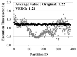
(a) PR – time

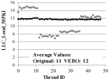
(b) PR – local misses

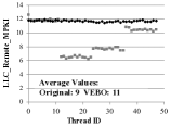
(c) PR – remote misses

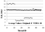
(d) PR – TLB

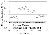
(e) PR – branches

Figure 4: Execution time and micro-architectural statistics per partition or per thread for PR with Twitter. Measured on GraphGrind using 384 partitions. Thread $t$ executes partitions $8\>t$ to $8\>t+7$. Architectural statistics expressed in misses per thousand instructions (MPKI).

V-C Random Permutation of Graphs

We evaluated the execution time of GraphGrind with four orders of vertex IDs: (a) original vertex IDs of a graph, (b) VEBO applied in original vertex IDs (c) a random permutation of the vertex IDs, and (d) VEBO applied to this random permutation. Evaluation on the Twitter and USAroad graphs (other graphs show similar trends) shows that the random permutation has higher execution time compared to the other orders (Figure 5). This occurs as a random permutation creates load imbalance. It also removes locality that may exist result from collecting the graph [21]. VEBO has lower execution time compared to the random permutations which demonstrates that VEBO is a sound algorithm and cannot be beaten easily by any permutation of vertices. Moreover, VEBO applied to the random permutation corrects load balance and restores performance to nearly the same level as VEBO applied to the original graph. The difference in performance, if any, can be attributed to differences in locality, which VEBO does not optimize.

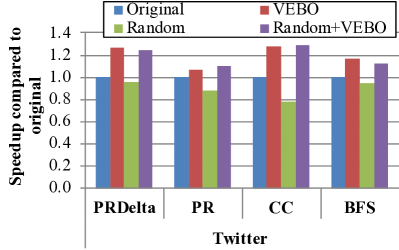
(a) Twitter

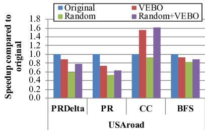
(b) USAroad

Figure 5: Performance of BFS on the Twitter and USAroad graphs using original vertex IDs, VEBO applied to original vertex IDs, a random permutation of the vertex IDs and VEBO applied to random vertex IDs. Execution times are normalised to the left-most case (original vertex IDs).

V-D Sparse Frontier

TABLE IV: Distribution of active edge over partitions for the sparse iteration in BFS of Twitter graph using 384 partition. S.D. is standard deviation value. Active Edge/Part is the ideal number of active edge per partition.

Iteration		3	4	5	6	7
Active Edge		7986019	6872249	636055	54173	5926
Active Edge/Part		20797	17896	1656	141.1	15.43
Min	Orig.	0	0	0	0	0
	VEBO	0	2533	194	5	0
Median	Orig.	541.5	13025	742.0	46.00	0.000
	VEBO	10114	16448	1486	127.0	11.00
S.D.	Orig.	79964	20539	3175	249.9	34.78
	VEBO	60525	16571	2462	170.5	25.93
Max	Orig.	1114127	148077	50780	3688	445
	VEBO	1112832	304976	44647	3216	370

Table IV shows distribution of active edge per iteration of BFS when using 384 partitions (distribution of active destination shows similar trends). Sparse frontiers vary strongly in size. The active edges per partitions is the optimization target as it corresponds to perfectly balanced partitions. VEBO distributes both high-degree and low-degree vertices uniformly over partitions. Compared to VEBO, original has many partitions with zero active degree. Iterations 3-7 dominate execution time during which the load balance is significantly improved by VEBO. VEBO reduces standard deviation up to 1.5x and it reduces the gap between minimum and maximum number of active edge per partition.

V-E Analysis of Load Balance

Figure 1 in Section II shows that VEBO balances edge and vertex counts. We show here that this load balance translates to run-time statistics. We focus on the PR algorithm for Twitter graph (Figure 4); the Friendster graph is similar, but not shown for brevity. We perform this analysis using GraphGrind.

Figure 4a shows the execution time for each of the 384 partitions. There is a large variation on the execution time for the original graph, e.g., from 0.290 s per iteration to 1.985 s. For the VEBO reordered graph (darkest symbols), the worst-case difference between the fastest and slowest partition is 0.17 s or more than 10 times less than the original graph. For most graphs and algorithms, the average time to process a partition is reduced by VEBO. This contributes to the speedup caused by VEBO, besides achieving load balance.

VEBO may reduce each partition’s performance but this is compensated by improved load balance. For instance, when processing PR for Twitter, the average execution time per partition is 1.211$\>s$ for VEBO with a 1.6x spread and 1.221$\>s$ for the original graph with a 6.9x spread.

VEBO balances execution at the micro-architectural level, namely miss rates for caches, TLBs and branch predictors (Figure 4). Moreover, we observed that VEBO improves memory locality for the majority of the graphs, as the cache and TLB statistics are reduced. PR for Twitter, however, is a rare counter-example.

Finally, VEBO reduces the branch misprediction rate (Figures 4e). We attribute this in part to ordering vertices by decreasing degree. When traversing the compressed sparse rows (CSR) and compressed sparse columns (CSC) data structures, a loop iterates over the edges incident to a vertex. The loop iteration count is determined by the degree. In the VEBO graph, subsequent vertices have the same degree which makes this branch highly predictable. In the original graph, subsequent vertices have highly varying degrees, which makes it hard to predict the loop termination accurately.

V-F Edgemap vs Vertexmap

TABLE V: Architectural events for vertexmap and edgemap: cache misses serviced from the local NUMA node, from the remote NUMA node (Rmt) and TLB misses. Numbers expressed as MPKI.

	App.	Order	Vertex Map			Edge Map
			Local	Rmt	TLB	Local	Rmt	TLB
Twitter	PR	Ori.	4.5	4.1	0.02	11.1	9.3	8.3
		VEBO	6.9	1.6	0.01	12.0	12.2	9.4
	BF	Ori.	2.5	2.0	0.03	9.1	11.0	11.5
		VEBO	3.6	0.5	0.01	8.9	10.6	11.2
Friendster	PR	Ori.	8.3	3.3	0.01	33.0	28.7	34.8
		VEBO	9.0	2.2	0.008	21.4	19.3	10.1
	BF	Ori.	6.0	1.5	0.02	27.0	20.5	23.6
		VEBO	6.6	0.8	0.01	22.6	16.7	20.2

Graph algorithms are expressed by means of edgemap and vertexmap traversals. VEBO simultaneously balances edges and vertices and so load balances both edgemap and vertexmap. The performance benefits are, however, different. Table V shows the summary statistics across the edgemap and vertexmap operations for Twitter and Friendster with PageRank (PR) and Bellman-Ford (BF). These statistics are collected per thread and correspond to the execution of 8 consecutive partitions. Edgemap generally dominates the execution time, so these statistics correspond closely to Figure 4. Local and remote cache misses as well as TLB misses are significantly reduced, except of PR for Twitter. VEBO generally improves memory locality during edgemap, even though this was not part of the optimization criterion.

Vertexmap benefits from load balancing rather than locality. GraphGrind spreads the iterations of the vertexmap loop equally across all threads [5]. Arrays accessed by vertexmap, however, are distributed over the NUMA nodes according to the graph partitions. This causes a high number of remote cache misses because Algorithm 1 induces imbalance in the number of vertices per partition. VEBO ensures that all partitions have an equal number of vertices. As such, each thread mostly accesses NUMA-local data, which explains the reduction in remote misses.

V-G Space Filling Curves

The dense frontiers of GraphGrind use the COO, which could be the same as if using CSR or CSC. Alternatively, ordering edges using the Hilbert space filling curve gives a significant performance boost [12]. However Hilbert order is a heuristic, which has been studied mostly for dense matrix algebra [22, 23].We have found that (i) there exist cases where Hilbert order degrades performance; (ii) the effectiveness of Hilbert order depends on the number of non-zeroes. To the best of our knowledge, neither of these properties are adequately covered in the literature.

We sort all vertices from high to low degree and partition the resulting graph into 384 partitions using Algorithm 1. We compare the performance of this high-to-low order against VEBO for PageRank (Figure 6a). The first partitions contain the vertices with the highest degrees, which are processed faster than a partition with a mix degrees of VEBO. The last partitions contain exclusively degree-one vertices and are processed up to three times slower than VEBO. This demonstrates that Hilbert order is more effective when the in-degree of vertices is high. High degrees imply more opportunity for reuse of data, which admit memory access order optimization.

Next,we compare Hilbert order to the traversal order of CSR, i.e., by increasing source vertex ID (Figure 6b). Surprisingly, the CSR order admits faster processing for partitions 0–350 (approximately). Thus, for high-degree vertices the CSR order is more efficient than Hilbert order.

As VEBO creates nearly the same degree distribution in each partition, it is expected that CSR order is more efficient than Hilbert order. We have modified GraphGrind accordingly to change COO using CSR order. This change consistently speeds up the algorithms with dense frontiers.

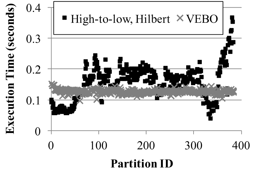
(a) High-to-low and VEBO

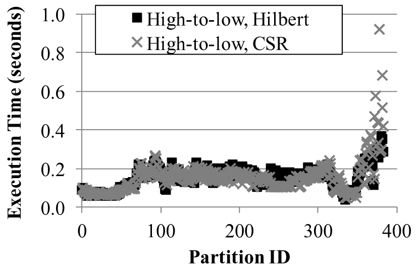
(b) Hilbert and CSR

Figure 6: Processing speed as a function of the in-degree. First iteration of PR on Twitter shown.

TABLE VI: Overhead in seconds of vertex reordering, edge reordering and partitioning for Twitter and Friendster compared to PR and BFS execution time. Fastest results in bold.

Graph	Vertex reordering			Edge reordering + partitioning		BFS		PR (50 iterations)
	RCM	Gorder	VEBO	Hilbert order	CSR order	Original	VEBO	Original	VEBO
Twitter	519.558	7803.871	5.119	10.684	4.412	0.245	0.210	59.122	48.465
Friendster	755.384	8930.228	11.164	13.482	5.441	0.931	0.513	147.220	76.532

V-H Overhead of Vertex Ordering

Table VI shows that VEBO reduces the cost of vertex ordering up to 101x over RCM and 1524x over Gorder. Moreover, VEBO performs best with CSR order for COO (Table III). This way of edge reordering and partitioning is faster than using Hilbert edge order: from 10.7s down to 4.4s for Twitter and 13.5s to 5.4s for Friendster. While graph preparation incurs some overhead, the overhead is far less than the gain. E.g., PR for Friendster takes 13.5s+147.2s on GraphGrind, while it takes 11.2s+5.4s+76.5s on GraphGrind with VEBO (PR typically requires over 50 iterations to converge). BFS traverses graphs from a single vertex, and has a significantly shorter execution time. However, in any reasonable setup multiple graph analytics would be performed each time a graph is loaded in memory such that the overhead of vertex and edge reordering can be amortized.

VI Related work

Graph partitioning has been thoroughly investigated. Graph partitioning problem is formulated as calculating a subset of the edges (or vertices) such that the number of edges crossing partitions is minimized [24, 4, 25, 26, 27]. Additionally, authors specify a constraint to balance the edges [28] or vertices [6, 1].

The exact solution to the graph partitioning problem is NP complete (e.g., [26]). Many authors have considered approximate algorithms to achieve a close-to-optimal solution in polynomial time [25, 26]. These may produce partitions of similar quality as general-purpose graph partitioners such as METIS [29] in less time [26].

One may partition the edge set or the vertex set. Partitioning the vertex set leads to a problem of minimizing the edge cut, potentially under a constraint of edge balance [2, 3, 4]. Partitioning the edge set leads to better heuristics and higher-performing implementations [1]. Edges now belong to a partition, while vertices may be replicated. In this problem, rather than minimizing the edge cut, the optimization criterion is to minimize the amount of vertex replication, also known as vertex cut.

Different graph partitioning approaches are used in distributed memory systems vs shared memory systems. Communication cost dominates distributed memory systems, hence edge cut and vertex replication are minimized [1, 30]. In shared memory systems, the best performing systems ensure that each partition contains vertices with consecutive vertex IDs. This simplifies indexing and improves memory locality. As such, partitioners such as METIS are not immediately applicable and additional vertex relabeling must be applied.

Streaming partitioning algorithms partition the graph in a single pass using a limited amount of storage [24, 27]. These algorithms compute approximations to the optimal partition of similar quality to METIS [29] in a fraction of the time [27]. Gonzalez et al proposed vertex cut, a parallel streaming partitioning algorithm that minimizes vertex replication [1]. Li et al [7] and Bourse et al [6] proposed efficient edge-balanced partitioning methods. Bourse et al [6] moreover investigate the interplay between edge balance and vertex balance, which is non-trivial if edge cuts are simultaneously minimized.

PowerLyra [30] differentiates ”high-degree” vertices from ”low-degree” vertices and applies different partitioning methods. It aims to minimize the replication factor. VEBO is different. It explicitly avoids minimizing replication factor and edge cut as this is computationally demanding. It is likely that VEBO can further improve PowerLyra because it is easier to minimize the edge cut when the high-degree vertices are processed first.

Graphs may be stored in multiple, equivalent ways. Vertex reordering aims to exploit the degree of freedom in vertex IDs. Gorder [10] proposes a general vertex ordering approach to improve CPU cache utilization. They find an optimal permutation among all nodes of a graph that retains temporal locality for nodes that are frequently accessed together. The RCM algorithm reduces the bandwidth of sparse matrices by relabeling vertices [9]. SlashBurn [31] exploits the hubs and their neighbours to define an alternative community different from the traditional community. LDG [24] is a heuristic streaming partitioner for large distributed graphs.

Edge reordering changes the order of edge traversal. Switching between CSR and CSC [17] is an edge reordering optimization. Space-filling curves tend to increase temporal locality [11]. Extensive partitioning (a.k.a. segmentation [32]) of CSR and CSC representations also improves temporal locality [12]. The interaction between vertex and edge reordering is not covered well in the literature.

VII Conclusion

The established heuristic to balance the processing time of graph partitions is to create edge-balanced partitions. We have demonstrated that edge-balance alone does not create good load balance and that considering vertex-balance along with edge-balance improves load balance significantly. Moreover, our results show that minimizing edge cut or vertex replication is not necessary on shared memory systems, and by extension on shared memory subsystems in distributed graph processing. We design VEBO, a vertex reordering algorithm for joint vertex and edge balancing and demonstrate that it achieves excellent load balance. for graphs with a power-law degree distribution.

We experimentally evaluated the performance of VEBO on three shared-memory graph processing systems: Ligra, Polymer and GraphGrind. Graph processing systems using static scheduling, such as Polymer and GraphGrind, benefit more strongly from VEBO.

In future work, we will investigate whether distributed graph processing systems, which typically use static scheduling, also benefit from increased load balance even if this comes at the expense of a small increase in vertex replication, and thus an increase in the volume of data communication. While VEBO improves load balance, there still remain unknown factors that affect the processing time of a graph partition. Identifying those factors may lead to still higher efficiency.

Appendix A Artifact Description Appendix: VEBO: A Vertex- and Edge-Balanced Ordering Heuristic to Load Balance Parallel Graph Processing

A-A Abstract

This description contains the information needed to launch some experiments of the paper ”VEBO: A Vertex- and Edge-Balanced Ordering Heuristic to Load Balance Parallel Graph Processing”. We explain how to compile and run the modified VEBO, GOrder and RCM in Ligra, Polymer and GraphGrind examples used in section IV. The results from section V are produced using NUMA-aware clang compiler, but this artifact description is not focused on that part of the paper.

A-B Description

A-B1 Check-list (artifact meta information)

• Algorithm: Graph ordering algorithm VEBO

• Program: C++ code with Cilkplus extension

• Compilation: icpc 14.0.0 and clang 3.4.1.

• Data set: Publicly available graph files in adjacency format.

• Run-time environment: Linux version 3.10.0-229.4.2.el7.x86_64

• Hardware: An x86-64 NUMA system.

• Output: VEBO generates reordered graphs with adjacency format and timing measurements (wall clock time) on data loading time and reordering time.

• Experimental workflow: Graph data sets are reordered with VEBO prior to loading in public graph processing frameworks (Ligra, Polymer and GraphGrind).

• Publicly available?: Yes, after publication of paper

A-B2 How software can be obtained (if available)

VEBO will be shared under open source license upon acceptance of the paper.

A-B3 Hardware dependencies

We use a 4-socket 2.6GHz Intel Xeon E7-4860 machine with 256GB of DRAM in our experiments.

A-B4 Software dependencies

VEBO is a stand-alone tool. Experiments make use of Ligra (https://github.com/jshun/ligra), Polymer (http://ipads.se.sjtu.edu.cn:1312/opensource/polymer.git), and GraphGrind (https://github.com/Jaiwen/GraphGrind). We compare against item GOrder and RCM (https://github.com/datourat/Gorder).

Ligra requires Cilkplus; GraphGrind requires a custom version of Cilkplus with NUMA extension. We have used the customized clang (https://github.com/hvdieren/swan_clang), LLVM (https://github.com/hvdieren/swan_llvm), and Cilkplus runtime (https://github.com/hvdieren/swan_runtime).

A-B5 Datasets

• Friendster, Orkut, LiveJournal are from Stanford Network Analysis Platform (SNAP). (http://snap.stanford.edu/snap/)

• Powerlaw graph is generated by snap-standford graph generator.(https://github.com/snap-stanford/snap/tree/master/examples/graphgen)

• RMAT27 graph is generated by Problem Based Benchmark Suite.(http://www.cs.cmu.edu/~pbbs/)

• Twitter is a social network graph from ”What is Twitter, a social network or a news media?” [14].

• Yahoo_mem is from Yahoo! Inc. (http://webscope.sandbox.yahoo.com)

• USAroad is from 9th DIMACS Implementation Challenge - Shortest Paths. (http://www.dis.uniroma1.it/challenge9/data/USA-road-d/USA-road-d.USA.gr.gz)

A-C Installation

Download VEBO and compiler using Cilkplus compiler, e.g.,

• clang++ 4.9.2 or higher with support for Cilkplus.

• Intel icpc compiler

Compiling VEBO: icpc -O3 -fcilkplus -g -c rMatGraph.C -o rMatGraph.o

A-D Experiment workflow

After downloading the package from XXXXX, install it using the above instruction. For reordering, run the tool using the following command: ./VEBO -r 100 -p 384 original vebo Where:

• r: start vertex to track in the new reordering graph

• p: number of graph partitions.

• original: file containing the original graph (input)

• vebo: file where reordered graph is stored

Output: A reordered graph using VEBO that is isomorphic to the original graph.

A-E Evaluation and expected result

The expected result is that the partitions of the reordered graph have a balanced number of vertices (unique destinations) and edges in each parition, i.e., in each 1/384-th set of vertices. It is expected that the reordered graph will be processed faster than the original graph with Polymer and GraphGrind when the graph is scale-free.

A-F Experiment customization

There is no need for customization to produce the results in this paper.

A-G Notes

None.

References

- [1] J. E. Gonzalez, Y. Low, H. Gu, D. Bickson, and C. Guestrin, “Powergraph: Distributed graph-parallel computation on natural graphs,” in OSDI, 2012.
- [2] A. Kyrola, G. E. Blelloch, and C. Guestrin, “GraphChi: Large-scale graph computation on just a PC.” in OSDI, 2012, pp. 31–46.
- [3] A. Roy, I. Mihailovic, and W. Zwaenepoel, “X-stream: Edge-centric graph processing using streaming partitions,” in Proc. of the ACM Symp. on Operating Systems Principles, 2013, pp. 472–488.
- [4] K. Zhang, R. Chen, and H. Chen, “NUMA-aware graph-structured analytics,” in Proc. of ACM Symp.on Principles and Practice of Parallel Programming, 2015, pp. 183–193.
- [5] J. Sun, H. Vandierendonck, and D. S. Nikolopoulos, “GraphGrind: Addressing load imbalance of graph partitioning,” in Proc. of ACM Intl. Conference on Supercomputing, 2017, pp. 16:1–16:10.
- [6] F. Bourse, M. Lelarge, and M. Vojnovic, “Balanced graph edge partition,” in Proc. of the ACM SIGKDD Intl.l Conf. on Knowledge Discovery and Data Mining, 2014, pp. 1456–1465.
- [7] R. Li, L.and Geda, A. B. Hayes, Y. Chen, E. Z. Chaudhari, P.and Zhang, and M. Szegedy, “A simple yet effective balanced edge partition model for parallel computing,” Proc. ACM Meas. Anal. Comput. Syst., pp. 14:1–14:21, 2017.
- [8] J. Shun and G. E. Blelloch, “Ligra: A lightweight graph processing framework for shared memory,” in Proc of ACM Symp. on Principles and Practice of Parallel Programming, 2013, pp. 135–146.
- [9] A. George, J. Liu, and E. Ng, “Computer solution of sparse linear systems,” 1994.
- [10] H. Wei, J. X. Yu, C. Lu, and X. Lin, “Speedup graph processing by graph ordering,” in Proc. of International Conference on Management of Data, ser. SIGMOD ’16. ACM, 2016, pp. 1813–1828.
- [11] D. G. Murray, F. McSherry, R. Isaacs, M. Isard, P. Barham, and M. Abadi, “Naiad: A timely dataflow system,” in Proc. of the ACM Symp. on Operating Systems Principles, 2013, pp. 439–455.
- [12] J. Sun, H. Vandierendonck, and D. S. Nikolopoulos, “Accelerating graph analytics by utilising the memory locality of graph partitioning,” in Proc of ICPP, 2017, pp. 181–190.
- [13] R. L. Graham, “Bounds on multiprocessing timing anomalies,” SIAM Journal on Applied Mathematics, pp. 416–429, 1969.
- [14] H. Kwak, C. Lee, H. Park, and S. Moon, “What is twitter, a social network or a news media?” in Proc. of the ACM intl. conference on World wide web, 2010, pp. 591–600.
- [15] Stanford. (2009) Stanford large network dataset collection. [Online]. Available: https://snap.stanford.edu/data/
- [16] L. Page, S. Brin, R. Motwani, and T. Winograd, “The pagerank citation ranking: Bringing order to the web.” Stanford InfoLab, Technical Report, 1999.
- [17] S. Beamer, K. Asanović, and D. Patterson, “Direction-optimizing breadth-first search,” in Proc. of the Intl. Conference on High Performance Computing, Networking, Storage and Analysis, 2012, pp. 12:1–12:10.
- [18] M. Frigo, C. E. Leiserson, and K. H. Randall, “The implementation of the Cilk-5 multithreaded language,” in Proc. of the ACM SIGPLAN conf. on Programming Language Design and Implementation, 1998, pp. 212–223.
- [19] Z. Chen, Y. Liu, R. C. Wong, J. Xiong, G. Mai, and C. Long, “Optimal location queries in road networks,” ACM Transactions on Database Systems (TODS), p. 17, 2015.
- [20] Y. Low, D. Bickson, J. Gonzalez, C. Guestrin, A. Kyrola, and J. M. Hellerstein, “Distributed graphlab: A framework for machine learning and data mining in the cloud,” Proc. VLDB Endow., vol. 5, no. 8, pp. 716–727, Apr. 2012.
- [21] F. McSherry, “A uniform approach to accelerated pagerank computation,” in Proceedings of the 14th International Conference on World Wide Web, ser. WWW ’05. New York, NY, USA: ACM, 2005, pp. 575–582. [Online]. Available: http://doi.acm.org/10.1145/1060745.1060829
- [22] C. Ding and K. Kennedy, “Improving cache performance in dynamic applications through data and computation reorganization at run time,” in Proc. of the ACM SIGPLAN Conf. on Programming Language Design and Implementation, 1999, pp. 229–241.
- [23] J. Mellor-Crummey, D. Whalley, and K. Kennedy, “Improving memory hierarchy performance for irregular applications using data and computation reorderings,” Intl. Journal of Parallel Programming, pp. 217–247, 2001.
- [24] I. Stanton and G. Kliot, “Streaming graph partitioning for large distributed graphs,” in Proc. of the ACM SIGKDD intl.l conference on Knowledge discovery and data mining, 2012, pp. 1222–1230.
- [25] K. Andreev and H. Racke, “Balanced graph partitioning,” Theory of Computing Systems, pp. 929–939, 2006.
- [26] U. Feige and R. Krauthgamer, “A polylogarithmic approximation of the minimum bisection,” SIAM Journal on Computing, pp. 1090–1118, 2002.
- [27] C. Tsourakakis, B. Gkantsidis, C.and Radunovic, and M. Vojnovic, “Fennel: Streaming graph partitioning for massive scale graphs,” in Proc. of ACM Intl. Conf. on WSDM, 2014, pp. 333–342.
- [28] G. Karypis and V. Kumar, “Multilevel algorithms for multi-constraint graph partitioning,” in Proc. of ACM/IEEE conference on Supercomputing, 1998, pp. 1–13.
- [29] ——, “Multilevel k-way partitioning scheme for irregular graphs,” Journal of Parallel and Distributed computing, vol. 48, no. 1, pp. 96–129, 1998.
- [30] R. Chen, J. Shi, Y. Chen, and H. Chen, “PowerLyra: Differentiated graph computation and partitioning on skewed graphs,” in Proceedings of the Tenth European Conference on Computer Systems, ser. EuroSys ’15. New York, NY, USA: ACM, 2015.
- [31] Y. Lim, U. Kang, and C. Faloutsos, “Slashburn: Graph compression and mining beyond caveman communities,” IEEE Trans. on Knowledge and Data Engineering, pp. 3077–3089, 2014.
- [32] Y. Zhang, V. Kiriansky, C. Mendis, M. Zaharia, and S. Amarasinghe, “Optimizing cache performance for graph analytics,” arXiv preprint arXiv:1608.01362, 2016.