Introduction to neutrino astronomy

Abstract

This paper is an introduction to neutrino astronomy, addressed to astronomers and written by astroparticle physicists. The focus is on achievements and goals in neutrino astronomy, rather than on the aspects connected to particle physics, however the particle physics concepts needed to understand the peculiar neutrino features are also introduced. The material is selected - i.e., not all achievements are reviewed - making however efforts to highlight current research issues.

The layout of this paper is as follows: In Sect. 1, we introduce the neutrinos, examine their interactions, and present neutrino detectors and telescopes. In Sect. 2, we discuss solar neutrinos, that have been detected and are matter of intense (theoretical and experimental) studies. In Sect. 3, we focus on supernova neutrinos, that inform us on a very dramatic astrophysical event and can tell us a lot on the phenomenon of gravitational collapse. In Sect. 4, we discuss the highest energy neutrinos, a very recent and lively research field. In Sect. 5, we review the phenomenon of neutrino oscillations and assess its relevance for neutrino astronomy. Finally, we offer a brief overall assessment and a summary in Sect. 6. In order to help the beginner, we prefer to limit the list of references, opting whenever possible for review works such as bahcall3 ; r1 ; r2 ; astro-book .

1 Neutrino properties and neutrino telescopes

1.1 General properties

Neutrinos are neutral particles which interact very rarely with matter; to have an idea of how small they are, if an atom were scaled to the size of the Earth (namely, if one zoomed in by a factor of about $10^{17}$) the atomic nucleus would have the size of a football field and solar neutrinos would have the size of one virus! Evidently it is not easy to “see” them.

There are 3 types of neutrinos, traditionally called ‘flavors’. They are identified by the charged particles that neutrinos can produce by interacting with matter. Such charged particles are the electron ($\mathrm{e}$), the muon ($\mu$), the tau ($\tau$), all with the same negative charge $-1$, in units of $1.602\times 10^{-19}$ Coulombs. For instance, an electron neutrino $\nu_{\mathrm{e}}$ is the neutral particle that, when interacting, can produce an electron; a muon neutrino $\nu_{\mu}$ can produce a muon, etc. Likewise, antineutrinos can be defined as those particles that can produce the various particles with charge $+1$; e.g., a tau antineutrino $\bar{\nu}_{\tau}$ produces an anti-tau, with mass equal to the tau particle. Using the formalism of chemical reactions, we will write

$$\nu_{\ell}+X\to\ell^{-}+Y\mbox{ with }\ell=\mathrm{e},\mu,\tau$$ (1)

where $X$ is an initial and $Y$ a final particle (or set of particles), and their electric charges are $Q(Y)=Q(X)+1$. Following the usual convention, we indicate neutrinos by the symbol $\nu$, and antineutrinos by $\bar{\nu}$. A brilliant pictorial summary of the main neutrino features can be found at the following web site:

http://www.quarked.org/askmarks/answer4.html

Note finally that, in the observations of neutrino astronomy, as a rule, neutrinos should be considered as individual particles rather than waves. In comparison to ordinary astronomy, it is as if neutrino astronomy were always in the single-photon mode. Peculiar wave phenomena, however, affect the propagation of neutrinos (see Sect. 5).

1.2 Neutrino interactions

Physicists quantify the probability of any interaction (or process) to take place by computing the corresponding “cross sections”, which can be interpreted as the transversal size of a target we would like to hit. The cross sections are usually indicated by the symbol $\sigma$. Quite in general, the cross section is linked to the number density of targets $n$ and to the mean free path $\lambda$ by the relation, $n\times\sigma\times\lambda=1$; if a particle travels a distance $d,$ one calls opacity the product $\tau=n\times\sigma\times d$, that quantifies the probability of no interaction

$$P(d)=\exp(-\tau)=\exp(-d/\lambda)$$ (2)

The estimation of the size of the neutrino $R_{\nu}$ given in the previous section is obtained by setting $\sigma_{\nu}\equiv\pi R^{2}_{\nu}$, where $\sigma_{\nu}$ is the typical cross-section of a process involving neutrinos. Such processes have cross-sections which are proportional to a universal constant

$$G_{F}^{2}=5.297\times 10^{-44}\mbox{ (cm/MeV)}^{2}$$ (3)

where $G_{F}$ is called Fermi constant. The vast majority of neutrino cross sections are therefore given by $G_{F}^{2}$ times the square of an energy or the product of an energy and a mass, simply for dimensional reasons. However, the theory links the interactions of the neutrinos with other observable processes: for instance, all reactions and decay processes listed in table 1 share the same dynamics. Note that all six reactions of table 1 can be obtained one from the other by either exchanging a particle from one side to the corresponding antiparticle in the other side of the reaction, or exchanging the direction of the arrow. The decay rates $\Gamma$, in particular, are also proportional to $G_{F}^{2}$; again, for dimensional reasons, this is multiplied by the fifth power of a mass.

Table 1: Most common reactions involving electronic neutrinos and antineutrinos with neutrons and protons ($n$ and $p$) and their traditional names: $\beta^{\pm}$ decay, electron (positron) capture, Inverse Beta Decay (IBD).

name	reaction
$\beta^{-}$ decay	$\mathrm{n}\to\mathrm{p}+\mathrm{e}^{-}+\bar{\nu}_{\mathrm{e}}$
$\beta^{+}$ decay	$\mathrm{p}\to\mathrm{n}+\mathrm{e}^{+}+\nu_{\mathrm{e}}$
$\beta^{-}$ capture	$\mathrm{p}+\mathrm{e}^{-}\to\mathrm{n}+\nu_{\mathrm{e}}$
$\beta^{+}$ capture	$\mathrm{n}+\mathrm{e}^{+}\to\mathrm{p}+\bar{\nu}_{\mathrm{e}}$
IBD	$\mathrm{p}+\bar{\nu}_{\mathrm{e}}\to\mathrm{n}+\mathrm{e}^{+}$
IBD on $n$	$\mathrm{n}+\nu_{\mathrm{e}}\to\mathrm{p}+\mathrm{e}^{-}$

1.3 Principles of neutrino detectors and telescopes

In view of the small chance of seeing these particles, it is quite evident that neutrino detectors need to have a large amount of target particles. Let us indicate their number by $N_{\mbox{\tiny target}}$ and consider an intense flux of neutrinos/antineutrinos, measured e.g., in $1/(\mbox{cm}^{2}\mbox{s})$, that we call $\Phi_{\nu}$. In the time of observation (or of emission) $T$, we will have that the number of observable events is:

$$\mathcal{N}_{\mbox{\tiny events}}=N_{\mbox{\tiny targets}}\times T\times\sigma\times\Phi_{\nu}$$ (4)

where $\sigma$ is the relevant cross section. In view of the above considerations, and more precisely of the smallness of the cross section, only a few specific sources of neutrinos can be observed. Three of them will be examined in the following three Sections; for a more complete list, see astro-book ; rev1 . Moreover, the number of events due to other processes, that can mimic neutrino-induced events (so called background processes) should be minimized. For this reason, neutrino observatories are located underground, underwater or under-ice, at a sufficient depth, so that the cosmic radiation and its byproducts are screened. On top of that, the neutrino detectors which aim at observing low-energy (MeV) neutrinos have to be sure that radioactive decays do not give an excessive amount of spurious events. In practice, this means that any neutrino detector has to restrict its observations only to those events that fall above a minimal energy (“threshold”) or that arrive at a certain time or from a certain direction of the sky.

Later, we will use the more specific term ‘neutrino telescope’ rather than the generic one ‘neutrino detector’ in the few cases when the detector can provide astronomers with information on the direction of arrival. However, note that, every so often, the two terms are just synonyms, see e.g., syn ; conversely, from time to time, ‘neutrino telescope’ is used in the narrow sense of ‘high energy neutrino telescope’, see e.g., a5 .

2 Solar neutrinos

In this section, we introduce the theoretical description of the solar neutrinos and examine the current observational knowledge. A few references that can help to access more deeply into these topics are bahcall3 ; r1 ; r2 ; astro-book ; r3 .

The understanding of the reason of solar energy took a lot of time. One early idea (Perrin, 1919, pero ) was that, in the reaction 4H$\to$He among atoms, the decrease in mass of $\sim 1$% liberates energy. In actuality, this happens through various sequences of nuclear transformations, where the net disappearance of 2 electrons is compensated by the appearance of 2 electron neutrinos.

In the Sun, the most important of such reactions is the proton-proton fusion ($\rm D=$ ²H nucleus):

$$\mathrm{p}+\mathrm{p}\to\mathrm{D}+\mathrm{e}^{+}+\nu_{\mathrm{e}}$$ (5)

This reaction is slow and occurs overcoming the electromagnetic repulsion of the protons, thanks to quantum tunnelling: this is why stars can live for billions of years.

The solar neutrinos, i.e., the neutrinos emitted by the Sun, are of physical interest for the many reasons:

1. they tell us how the Sun works, which is important on its own and also for the stellar physics at large;

2. neutrinos escape from the Sun in about 2 seconds, rather than some $100,000$ years as the photons do: they are real-time messengers from the Sun;

3. the measurements of solar-neutrino flavor-oscillations give clear evidence of physics beyond the standard model of particle physics.

The neutrinos produced by the reaction in Eq. (5) are the most abundant ones and are called pp neutrinos.

2.1 The Standard Solar Model and its tests

An essential contribution to the study of solar neutrinos - e.g., bahcall3 ; bahcall1 ; bahcall2 - is due to John Bahcall, a nuclear physicist who came up with what nowadays is called the Standard Solar Model (SSM). Very roughly, the SSM consists in a physical description of the composition of the Sun and of the processes which make it work.

Using such model, Bahcall could predict the rate of neutrinos from the Sun and thus set a benchmark for the Homestake experiment (1967-1995), which resulted in the first solar neutrino detection for which Raymond Davis Jr. was awarded a Nobel prize homestake . However, the number of neutrinos measured by Davis’ experiment resulted to be only 1/3 of that predicted by Bahcall, so that both physicists felt compelled to check their procedures. Their goal was indeed very tough (and even today solar neutrino detection and modelling is far from easy): on the one hand the SSM is based on models of the metallicity, opacity and of nuclear processes of the Sun (and tested by helioseismology), but on the other hand neutrinos interact so weakly that their detection rate is small and a very high radiopurity (knowledge and reduction of the sources of background) is mandatory.

Today we know that the Homestake experiment was right, as it was sensitive to one neutrino flavor, $\nu_{\mathrm{e}}$, being based on the electron neutrino capture process:

$$\nu_{\mathrm{e}}+\mathrm{\textsuperscript{37}Cl}\to\mathrm{\textsuperscript{37}Ar}+\mathrm{e}^{-}$$ (6)

Instead, newer experiments as Borexino, SNO and Super-Kamiokande can (could) detect neutrinos via their elastic scattering off electrons:

$$\nu+\mathrm{e}^{-}\to\nu+\mathrm{e}^{-}$$ (7)

and thus are (were) sensitive to all flavors of (anti)neutrinos. This is why we used the generic notation $\nu$ for neutrinos here above. This is even more true for the most important measurement of the SNO experiment, that was equally sensitive to all three types of neutrinos, and that has been recognized by the Nobel award.

To give an idea of how complex and interesting the physics of the Sun is, new and more refined versions of the Standard Solar Models are put forward almost every year. The last one is latestsolarmodel , published in 2017.

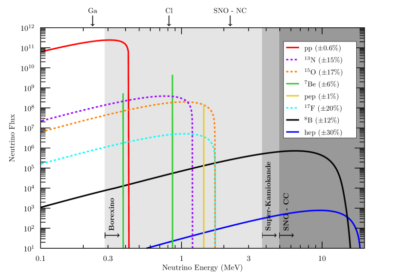
Figure 1: Energy dependence of the neutrino fluxes produced by the different nuclear processes in the Sun, according to the B16-GS98 Standard Solar Model latestsolarmodel . The $y$ axis is in units of cm^-2 s^-1 MeV^-1 for continuous spectra and cm^-2 s^-1 for monochromatic ones (beryllium and $\mathrm{p}\mathrm{e}\mathrm{p}$ neutrinos). The neutrino energy threshold for detection is indicated with a vertical arrow for the experiments which do not reconstruct the neutrino energy (those based on gallium, as GALLEX/GNO and SAGE, on chlorine, as Homestake, or on neutral current $\nu$-D interactions, as SNO) and with a horizontal arrow for those which reconstruct the neutrino energy (those based on elastic scattering, as Borexino and Super-Kamiokande, and on charged current $\nu$-D interactions, as SNO). The dashed lines highlight the CNO-cycle contribution to the solar neutrino flux.

2.2 The pp neutrino flux and their detection

The nuclear reaction in Eq. (5) begins a set of reaction called $\mathrm{p}\mathrm{p}$ chain: the SSM predicts that the $\mathrm{p}\mathrm{p}$ chain is the main channel of energy and neutrino production, as reported in Table 2 and as evident from figure 1.

Table 2: SSM expectations of the solar neutrinos arriving at Earth, due to the various branches of neutrino production latestsolarmodel . The first 5 neutrinos are those of pp-chain (all observed except the last); the last 3 are those of the CNO-cycle (yet unobserved).

branch		flux, $10^{6}/$(cm2 s)	$E_{\nu}^{\text{\tiny max}}$, MeV
$\mathrm{p}\mathrm{p}$		$59,800(1\pm 0.006)$	0.420
7Be		$4,930(1\pm 0.06)$	0.862
$\mathrm{p}\mathrm{e}\mathrm{p}$		$144(1\pm 0.01)$	1.442
8B		$5.46(1\pm 0.12)$	15.1
$\mathrm{h}\mathrm{e}\mathrm{p}$		$0.008(1\pm 0.30)$	18.773
13N		$278(1\pm 0.15)$	1.199
15O		$205(1\pm 0.17)$	1.732
17F		$5.28(1\pm 0.20)$	1.740

The $\mathrm{p}\mathrm{p}$ neutrinos amount to more than 90% of the solar neutrino flux coming to Earth.

The flux can be roughly estimated by elementary considerations: We know that a nucleus of Helium is formed after two $\mathrm{p}\mathrm{p}$ fusions, so that:

$$\dot{N}_{\mathrm{p}\mathrm{p}}\simeq 2\dot{N}_{\mathrm{He}}$$ (8)

Moreover, we know that $Q=26.7\;$MeV are produced in the production of Helium, which implies

$$\dot{N}_{\mathrm{He}}\simeq\frac{L_{\odot}}{Q}\simeq 10^{38}\,\mathrm{Hz}$$ (9)

In this manner, we obtain an estimate of the flux,

$$\Phi_{\nu_{\mathrm{e}}}\simeq\frac{2\dot{N}_{\mathrm{He}}}{4\pi(1\;\mathrm{AU})^{2}}\simeq 6\times 10^{10}\;\mathrm{cm}^{-2}\,\mathrm{s}^{-1}$$ (10)

This flux is sizeable, but, considering experiments which detect neutrinos via elastic scattering of Eq. (7), we need to keep in mind that the probability of interaction (cross-section) of neutrinos with electrons is extremely small, even though theoretically very clean: for the cases of our concern, it grows with the square of the neutrino energy $E_{\nu}^{2}$. This means that, despite such a huge flux of $\mathrm{p}\mathrm{p}$ neutrinos, it is very difficult to detect them, and in fact their detection is recent borexpp . Moreover, neutrino-electron scattering detection has a threshold (on the recoil kinetic energy of the scattered electron) as low as 150 keV (in Borexino) with a neutrino energy reconstruction accuracy of the order of few percent.

Neutrino detection in Borexino is in fact based on the scintillation light emitted by the electron on which the neutrino impinged; Cherenkov detection has been discarded due to its very small light yield compared to that of scintillation (a few %). Since the scintillation light is emitted isotropically, direction reconstruction is not feasible / is very very difficult in this type of detectors, even in the case of elastic scattering Eq. (7).

Moreover, neutrino-induced events in liquid scintillators are intrinsically indistinguishable on an event-by-event basis from the background due to $\beta$ or $\gamma$ decays: this is why radiopurity is a key factor of this kind of experiments, aimed at finding rare neutrino events at very low energies.

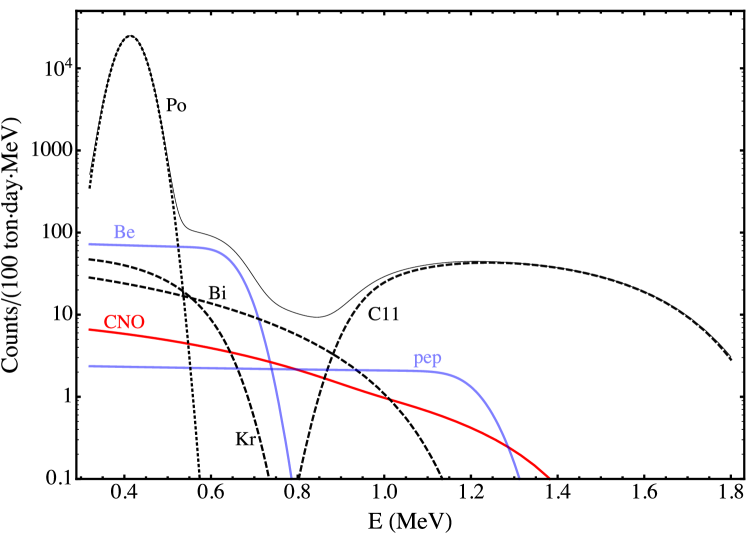
Figure 2: The differential rate of events in Borexino - inclusive of the background - as a function of the electron recoil kinetic energy. The continuous lines are the signals due to solar neutrinos; the CNO neutrinos indicated by a red line, the neutrinos from the PP chain are indicated by blue lines. The dotted and dashed black lines are due to background events instead. Particularly evident is the importance of a good knowledge of the bismuth background in order to detect CNO neutrinos. Figure adapted from vborex .

2.3 What we (do not) know

Once again, the state of the art of solar neutrino expectations is summarized in table 2 and figure 1.

For what concerns the measurements, we emphasize that the reconstruction of the energy of the solar neutrinos is important to test our understanding of how the Sun works. Super-Kamiokande and SNO measured accurately the ⁸B neutrinos, which are relatively more easy to be observed but are a very small fraction ($\sim$0.02%) of the SSM neutrino flux. Borexino experiment observed directly pp, pep, and ⁷Be neutrinos, measuring the latter precisely. We have only upper bounds on the very rare hep neutrinos–see again table 2.

In short, most of the neutrinos from the pp-chain have been measured, while those from the CNO cycle are not. The CNO cycle in the Sun is expected to yield $\sim 1$% of the solar luminosity, but it is very important for astronomy, being the main cycle of energy production in massive stars. It begins with a set of reactions called CNO-I cycle,

$$\phantom{centramiiiiiiii}\phantom{.}{}^{12}\mathrm{C}+\mathrm{p} \to\phantom{.}^{13}\mathrm{N}+\gamma$$

$$\phantom{.}{}^{13}\mathrm{N} \to\phantom{.}^{13}\mathrm{C}+\mathrm{e}^{+}+\nu_{\mathrm{e}}$$

$$\phantom{.}{}^{13}\mathrm{C}+\mathrm{p} \to\phantom{.}^{14}\mathrm{N}+\gamma$$

$$\phantom{.}{}^{14}\mathrm{N}+\mathrm{p} \to\phantom{.}^{15}\mathrm{O}+\gamma$$

$$\phantom{.}{}^{15}\mathrm{O} \to\phantom{.}^{15}\mathrm{N}+\mathrm{e}^{+}+\nu_{\mathrm{e}}$$

$$\phantom{.}{}^{15}\mathrm{N}+\mathrm{p} \to\phantom{.}^{12}\mathrm{C}+\phantom{.}^{4}\mathrm{He}$$

As we can see, CNO-I yields neutrinos from the $\beta^{+}$ decay of ${}^{13}\mathrm{N}$ and ${}^{15}\mathrm{O}$. Replacing the last reaction of $\alpha$ emission with $\gamma$ emission we begin the CNO-II cycle, that is much less frequent in our Sun,

$$\phantom{centramiiiiiiii}\phantom{.}{}^{15}\mathrm{N}+\mathrm{p} \to\phantom{.}^{16}\mathrm{O}+\gamma$$

$$\phantom{.}{}^{16}\mathrm{O}+\mathrm{p} \to\phantom{.}^{17}\mathrm{F}+\gamma$$

$$\phantom{.}{}^{17}\mathrm{F} \to\phantom{.}^{17}\mathrm{O}+\mathrm{e}^{+}+\nu_{\mathrm{e}}$$

$$\phantom{.}{}^{17}\mathrm{O}+\mathrm{p} \to\phantom{.}^{14}\mathrm{N}+\phantom{.}^{4}\mathrm{He}$$

Also this cycle yields one type of neutrinos, due to $\beta^{+}$ decay of ${}^{17}\mathrm{F}$. Finally, there are also CNO-III and CNO-IV cycles, important only for very massive stars.

CNO neutrinos offer us a chance to understand the CNO cycle and Borexino has a chance to see them for the first time; unfortunately, this measurement represents a true challenge, as can be understood from figure 2. The $\beta$ decay of bismuth (one of the daughters of radon) is the main reason of background events. However, it is associated to the $\alpha$ decay of polonium vborex , that leads to events visible on the left hand side of figure 2

$${}^{210}\mbox{Bi}\stackrel{{\scriptstyle\mbox{\tiny 7d}}}{{\longrightarrow}}{}^{210}\mbox{Po}+\mbox{e}^{-}+\bar{\nu}_{\mbox{\tiny e}}\stackrel{{\scriptstyle\mbox{\tiny 200d}}}{{\longrightarrow}}{}^{206}\mbox{Pb}+\alpha$$ (11)

In stable conditions, the decay events follow the law of radioactive decay which should allow to measure the bismuth from polonium vborex . Borexino has the chance to measure CNO neutrinos in a few years applying a dedicated analysis.

3 Supernova neutrinos

Neutrinos emitted during the gravitational collapse, associated to a visible supernova of a certain astronomical type, are called for short supernova neutrinos. The astrophysics is much more complicated than that of solar neutrino emission, the associated uncertainties are large and the theorists involved in the study of this type of events are still unsure whether their computer simulations include all the relevant physics.

However, 30 years ago we had a successful observation of the neutrinos from one supernova, called SN 1987 A, that has been recognized by the 2002 Nobel prize in physics to the Koshiba, the leader of the Kamiokande experiment.

In order to provide an introduction to this interesting and complex subject, we will focus the discussion on basic features of neutron stars and of the gravitational collapse; on expectations about the neutrino emission; on the signal of electron antineutrinos in detectors devoted to monitor supernova emission, with a brief mention of the events from SN1987A. For further general discussion, see astro-book ; rev1 ; for a specialized discussion on SN1987A, see Vissani:2014doa .

3.1 The supernova - neutron star connection

Supernovae have been occasionally observed in the past centuries. In 1933, just after the discovery of the neutron, Baade and Zwicky proposed the idea that this observable astronomical phenomenon is connected with the formation of a very compact object: a large fraction of the stellar mass gets transformed from ordinary atomic matter into neutrons. In other words, the size, typically occupied by matter, decreases from the one corresponding to atoms, $R_{\mbox{\tiny atomic}}\sim 10^{-8}$ cm to the one corresponding to nuclei, $R_{\mbox{\tiny nucl}}\sim 10^{-13}$ $\mathrm{cm}=1$ fermi, namely, it would decrease by $R_{\mbox{\tiny atomic}}/R_{\mbox{\tiny nucl}}\sim 10^{5}$ times. For example, our Sun would fit in a region of $700\,000$ km/$10^{5}\sim$ 7 km!

Indeed, the typical radius of a neutron star (estimated by using general relativity and the theory of strong interactions) is $R_{\mathrm{ns}}=10-15$ km. On the other hand, its typical (measured) mass is $M_{\mathrm{ns}}\geq 1.44\,M_{\odot}$ or larger, which is the maximum mass of a white dwarf before that it collapses under its weight. The existence of such a limiting mass was predicted in 1930 by Chandrasekhar.

The gravitational binding energy $\mathcal{E}$ of the neutron star is huge:

$$\mathcal{E}\sim\frac{3}{5}\frac{G_{\mathrm{N}}M_{\mathrm{ns}}^{2}}{R_{\mathrm{ns}}}=(2-3)\times 10^{53}\,\mathrm{erg}$$ (12)

where of course $G_{\mathrm{N}}\sim 7\times 10^{-8}$ erg cm/g² is the Newton constant. This is a significant (10-15%) fraction of the rest mass $M_{\mathrm{ns}}c^{2}$; in order to allow the formation of the neutron star, this energy should be released. The main agents which are able to carry away such tremendous amount of energy in a short time are just neutrinos. In fact, these particles are copiously produced during and immediately after the collapse of the star, and can escape from the star rapidly enough.

In order to better picture how this happens, consider the opacity of neutrinos crossing the neutron star:

$$\tau=\rho/m_{N}\times\sigma\times R_{\mathrm{ns}}$$ (13)

With a cross section of $\sigma\sim 10^{-41}$ cm², with a density of $\rho=10^{11}$ g/cm³, with a radius of 10 km, we have $\tau\sim 10^{11}\times 6\cdot 10^{23}\times 10^{-41}\times 10^{6}\sim 1$, which means that the external regions of the neutron star are transparent and allow neutrinos to escape. In the innermost parts of the neutron star, however, we have $\sim 1$ particle/fermi³. Thus the density is $\rho\sim$few$\times 10^{14}$ g/cm³, and neutrinos are trapped in the region where they are produced. The cross section $\sigma\sim 10^{-41}$ cm² corresponds to neutrinos with energies of $10-20$ MeV. The surface of the star, where neutrinos are radiated, is called neutrinosphere and can be thought of, in a first approximation, as a black body radiator.

The sequence of the events, which leads to the formation of a neutron star, is as follows;

1. in the largest stars (above 6-10 $M_{\odot}$) a chain of nuclear reactions leads to form a core of iron, that is stable with respect to further reactions;

2. when the core reaches the Chandrasekhar mass, the electrons become relativistic and the associated pressure is unable to support the core, that collapses under its weight;

3. the radius becomes 10 km, and the pressure of the neutrons provides stability to the new configuration;

4. the huge potential energy is radiated in neutrinos of all types, with energies around 10-20 MeV.

A small fraction of this energy, much less than Eq. (12), is converted then into kinetic energy. Indeed, the masses of gas expelled by a supernova are observed to have kinetic energies of the order of $Mv^{2}/2=10^{51}$ erg, which corresponds to a mass of $M\sim 10\ M_{\odot}$ moving at a velocity of $v\sim 3,000$ km/s. However the details of how this conversion takes place are not reliably known yet.

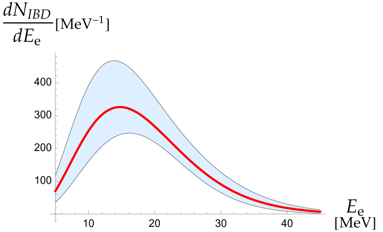
Figure 3: Expected distribution ($=$ spectrum) of the IBD signal due to electron antineutrinos, for a future galactic supernova exploding at 10 kpc and for a neutrino detector comprising $2.1\times 10^{33}$ protons–e.g., 32 kton of water or 29 kton of linear alkyl benzene. The expectations and the uncertainties are modeled on SN1987A data, see astro-book ; Vissani:2014doa for details.

3.2 The expected neutrinos

Let us begin by estimating the time scale of emission. The 6 types of neutrinos and antineutrinos are supposed to carry away the surplus of energy, thereby allowing the formation of the neutron star. Let us assume that (most of) them are emitted close to the surface of the proto-neutron star simply as black body radiation, and moreover that the temperature of each type of (anti)neutrinos is close to $T_{\nu}\sim 4$ MeV. The luminosity (=the radiated power) per neutrino type can be directly estimated from the Stefan-Boltzmann law:

$$L_{\nu}\approx R_{\mathrm{pns}}^{2}\times T_{\nu}^{4}\mbox{ with }\nu=\nu_{\mbox{\tiny e}},\nu_{\mu},\nu_{\tau},\bar{\nu}_{\mbox{\tiny e}},\bar{\nu}_{\mu},\bar{\nu}_{\tau}$$ (14)

where the radius of the proto-neutron star is around $R_{\mathrm{pns}}\sim 15$ km. By including the dimensional constants $c=3\times 10^{10}$ cm/s and $\hbar c=200$ MeV$\times$fermi, the value of the luminosity in conventional units turns out to be:

$$L_{\mathrm{tot}}=6\times L_{\nu}\approx 2\times 10^{52}\text{erg s}^{-1}$$ (15)

Thus, the whole potential energy of the star is gone in a time $\mathcal{E}/L_{\mathrm{tot}}$, namely, 10 seconds or so.

Next, we would like to estimate the neutrino fluence on Earth, i.e. the flux integrated over the time of emission. Let us begin by calculating the number of neutrinos, that for each species ($\nu_{\mathrm{e}},\nu_{\mu},\nu_{\tau},\bar{\nu}_{\mathrm{e}},\bar{\nu}_{\mu},\bar{\nu}_{\tau}$) is

$$N_{\nu}=\frac{\mathcal{E}}{6\langle E_{\nu}\rangle}\approx\frac{3\times 10^{53}}{6\times 10}\frac{\mathrm{erg}}{\mathrm{MeV}}\approx\mathrm{few}\times 10^{57}\frac{\mathrm{erg}}{\mathrm{MeV}}$$ (16)

For comparison, we note that the number of electrons in the iron core (i.e., the electronic lepton number of the collapsing object) is,

$$N_{\mathrm{e}}=\frac{Y_{\mathrm{e}}\;M_{\mathrm{core}}}{m_{N}}=0.4\times 3\times 10^{33}\times 6\times 10^{23}=7\times 10^{56}$$ (17)

namely, it is more than one order of magnitude smaller than the total number of emitted neutrinos. Using as benchmark a distance of $D=10$ kpc, which is a typical galactic scale, we find that the neutrinos distribute on the surface of a sphere with area $S=4\pi D^{2}=10^{46}$ cm² before reaching the Earth, and therefore, we have,

$$F_{\nu}=\frac{N_{\nu}}{S}=\mathrm{few}\times 10^{11}\frac{\nu}{\mathrm{cm}^{2}}$$ (18)

where we recall that the time-integrated flux $F_{\nu}=\int\Phi_{\nu}(t)dt$ is called the fluence.

3.3 The IBD signal, SN1987A and the future

The type of neutrinos that has the largest probability of interaction with ordinary matter are the electron antineutrinos. The relevant reaction is in fact the one that has been first considered for the detection, that is sometimes called “inverse beta decay” (IBD), namely:

$$\overline{\nu}_{\mathrm{e}}+\mathrm{p}\to\mathrm{n}+\mathrm{e}^{+}$$ (19)

where the interaction happens with a proton, i.e., a nucleus of hydrogen. A typical value of the cross section at the relevant energies is $\sigma_{\mbox{\tiny IBD}}\sim 1.5\times 10^{-41}$ cm². If we consider the detector Super-Kamiokande sk , that has 22.5 kton of water, we have that the number of target protons is $N_{\mathrm{p}}=1.5\times 10^{33}$. Therefore, using the fluence $F_{\overline{\nu}_{\mathrm{e}}}=2\times 10^{11}\ \overline{\nu}_{\mathrm{e}}/$cm² estimated above for a supernova at 10 kpc, we find that the expected number of positrons $\mathrm{e}^{+}$ due to the IBD reaction is:

$$N_{\mathrm{e}^{+}}=N_{\mathrm{p}}\times\sigma_{\mbox{\tiny IBD}}\times F_{\bar{\nu}_{\mathrm{e}}}\approx 4,500$$ (20)

which is about 200 times larger than what was seen in the case of SN1987A. For an accurate prediction including uncertainties see Fig. 3, adapted from ref. astro-book .

Before leaving this topic, it should be recalled that the number of events seen from SN1987A in the same time window was small: 12 in Kamiokande, 8 in IMB, 5 in Baksan. In all cases, the emission lasts about 10 seconds and almost half of the IBD events (6, 3 and 2 respectively) happened in first second: this is consistent with the simulations, and will be one of the most interesting things to test with a future event.

Another very important thing that we hope to measure in the future with Super-Kamiokande sk is the sample of events from the neutrino scattering off atomic electrons introduced in Eq. (7) for solar neutrinos. This is a directional reaction, i.e., the electrons are emitted from the direction of arrival of the neutrinos within some tens of degree for each individual event. This will allow a few degrees reconstruction of the supernova position, see e.g., astro-book . Moreover, this reaction is not exclusively sensitive to $\overline{\nu}_{\mathrm{e}}$ (as in the case of IBD) but also to $\nu_{\mathrm{e}},\nu_{\mu},\nu_{\tau},\overline{\nu}_{\mu},\overline{\nu}_{\tau}$.

4 High energy cosmic neutrinos

Before discussing high energy cosmic neutrinos we have to know what are the different backgrounds that can make their detection difficult (sec. 4.1). Then we discuss theoretical expectations on the cosmic neutrino flux (sec. 4.2). We discuss the possible signals in neutrino detector and telescopes and the observational opportunities (secs. 4.3-4.4). Finally, we examine in the appendix the connection between neutrino and ordinary astronomy. For a few general references, see astro-book ; baur ; mau ; ger ; to go deeper into the subject, see the specialized review works a5 ; a1 ; a2 ; a3 ; a4 ; a6 ; a7 ; a8 .

4.1 High energy neutrinos of atmospheric origin

Neutrinos of high energy are produced in our atmosphere. In fact, atmospheric neutrinos come from the decay of unstable particles (mesons) produced by the cosmic ray bombardment that hits our atmosphere; these unstable particles have an energy that extends on average from 100 MeV up to many TeV. The atmosphere acts initially as a converter, that degrades the energy of the primary nucleons $N_{\mbox{\tiny cr}}$ producing mesons and eventually secondary particles

$$N_{\mathrm{cr}}+N_{\mathrm{atm}}\to X+\text{\small many mesons}\left\{\begin{array}[]{l}\pi^{0}\to\gamma+\gamma\\[4.30554pt] \pi^{\pm}\to\mu^{\pm}+\mathrel{\mathop{\nu}\limits^{\vbox to1.05487pt{\kern-2.0pt\hbox{$\scriptstyle\scalebox{0.3}{(}\raisebox{-1.7pt}{$-$}\scalebox{0.3}{)}$}\vss}}}_{\mu}\end{array}\right.$$ (21)

The $\gamma$-rays of high energy are screened by the atmosphere itself, while neutrinos and high-energy muons reach the ground and are observable. The path length of the muon is $\gamma_{\mu}\tau_{\mu}c=(E_{\mu}/m_{\mu})\times 0.6$ km, therefore when their energy is above 10 GeV, muons reach the ground before decaying, and the neutrinos that we receive on Earth are just the $\mathrel{\mathop{\nu}\limits^{\vbox to1.05487pt{\kern-2.0pt\hbox{$\scriptstyle\scalebox{0.3}{(}\raisebox{-1.7pt}{$-$}\scalebox{0.3}{)}$}\vss}}}_{\mu}$ of Eq. (21).

The neutrino spectrum behaves as $\sim E_{\nu}^{-2.7}$ at low energies, up to few GeV, just as the primary cosmic rays; then it becomes steeper for the following reason. Charged pions with more than 10 GeV have a Lorentz factor of $\gamma_{\pi}>70$ and travel $\gamma_{\pi}\tau_{\pi}c>0.4$ km. Now, let us calculate the interaction length. For an atmospheric density of about $\rho=10^{-3}$ g/cm³ and for a nuclear interaction cross section $\sigma_{n}=\pi r_{n}^{2}$ corresponding to a radius of $r_{n}=1$ fm, we have a mean free path of $\lambda_{n}=1/(N_{A}\rho\sigma_{n})=0.5$ km, where $N_{A}$ is the Avogadro number. Therefore, the higher the pion energy, the smaller their chance to decay before losing a significant fraction of energy. For this reason, atmospheric neutrinos are distributed as $\sim E_{\nu}^{-3.7}$ in the region 100 GeV-100 TeV and depleted at higher energies.

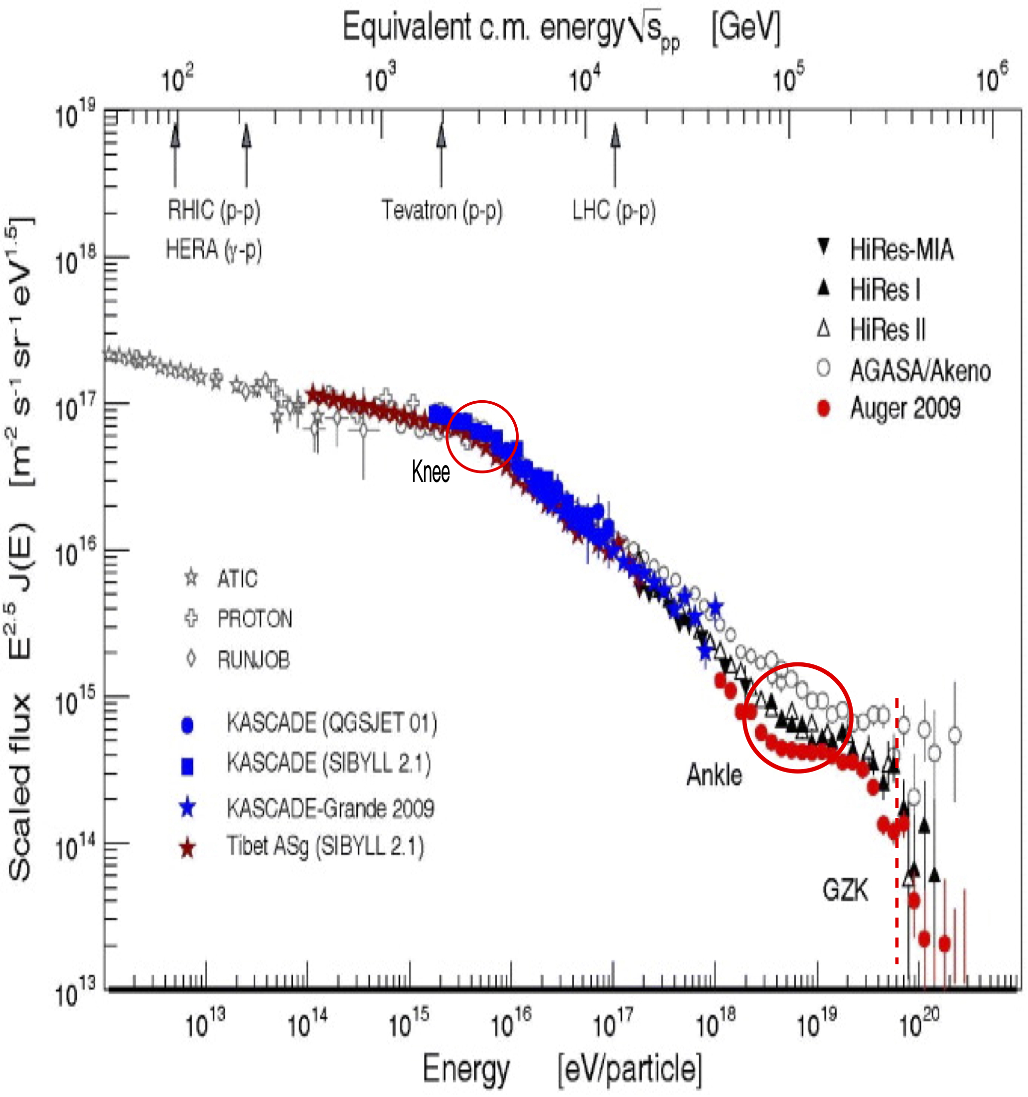
Figure 4: The cosmic ray spectrum, slightly modified version of figure 2 of matthiae .

The most energetic pions carry away $\sim 1/5$ of the energy of the primary, then every decay particle carries away, on average, a similar amount of energy. There are two $\gamma$-rays for the $\pi^{0}$ decay and four particles for the full decay of the $\pi^{\pm}$, since $\mu^{\pm}\to\mathrm{e}^{\pm}+\mathrel{\mathop{\nu}\limits^{\vbox to1.05487pt{\kern-2.0pt\hbox{$\scriptstyle\scalebox{0.3}{(}\raisebox{-1.7pt}{$-$}\scalebox{0.3}{)}$}\vss}}}_{\mathrm{e}}+\mathrel{\mathop{\nu}\limits^{\vbox to1.05487pt{\kern-2.0pt\hbox{$\scriptstyle\scalebox{0.3}{(}\raisebox{-1.7pt}{$-$}\scalebox{0.3}{)}$}\vss}}}_{\mu}$ so, on average, the photons are twice as energetic as the corresponding neutrinos. Thus, each $\gamma$-ray carries away about 1/10 of the primary energy, while this fraction becomes 1/20 for the neutrino.

Recalling that the cosmic ray spectrum shown in figure 4 at Earth softens above the knee, with $E_{\mathrm{knee}}=$ few PeV, we expect that the atmospheric neutrino spectrum extends up to

$$\frac{E_{\mathrm{knee}}}{20}\sim 100\mbox{ TeV}$$ (22)

For higher energies, the sky should become more and more free from atmospheric background events; thus, the high energy neutrinos could reveal the sources of the cosmic rays. The region below few 100 TeV is polluted by atmospheric neutrinos (and muons), but it is also important – in particular for the search of the sources of galactic cosmic rays, that are usually believed to have energies lower than the knee.

Not only pions and kaons, but also charmed particles are produced in pairs in cosmic ray collisions. Even if they are less common than pions, their lifetime is so short that they immediately decay and yield a spectrum of prompt neutrinos with shape $\sim E_{\nu}^{-2.7}$ that reflect the cosmic rays that impinge on atmosphere. Thus, somewhere at high energies the contribution of this component should exceed the one due to pions and kaons; this should happen around 100 TeV, even if the theoretical estimations are not stable enough to provide a solid prediction. Two main search strategies are possible:

1. the prompt neutrino spectrum (whose shape is assumed to be known) is fitted to the muon neutrino flux in order to extract the normalization of the prompt neutrino spectrum - and this is currently implemented in IceCube;

2. the other strategy is based on the study of the electron neutrino component, that is as abundant as that of muon neutrinos coming from the decay of charmed particles, (prompt) whereas it constitutes only 5% of the conventional (from the decay of pions and kaons) fluxes.

Prompt neutrinos have not been detected yet, and are thought to provide only few events in the detector; the bound currently obtained by IceCube already rules out the most optimistic predictions. Thus, there are chances to see high energy cosmic neutrinos over the atmospheric ones.

4.2 Sources of cosmic neutrinos

Although we do not have yet a clear theoretical idea on which the sources of cosmic neutrinos are and how intense they are, there are several ideas on the subject. In this section, we examine the case that the cosmic neutrinos are directly connected to the (sources of the) cosmic rays. In the appendix, we elaborate the connection between neutrinos and gamma rays.

Cosmic rays and cosmic neutrinos:–

Consider some astrophysical site where cosmic rays are produced and confined for some time. Suppose that there is some target (say, gas) for the cosmic rays to interact with. Moreover, let us begin by considering the case of this target being much more diffuse than Earth’s atmosphere. We might imagine that this site will be particularly brilliant in neutrinos and $\gamma$-rays, and that the shape of these secondary particles will reflect the production spectra of cosmic rays. The cosmic ray spectrum in the source is unknown a priori, however, there is one general theoretical argument in support of the idea that the spectrum behaves as $\sim E_{\mathrm{cr}}^{-2}$, both for $\gamma$-rays and for neutrinos. 1) First of all, such a spectrum is expected in the Fermi acceleration mechanism. 2) Second, if–just in the terrestrial atmosphere–the target for the cosmic ray collisions is composed by protons or other nuclei, but–differently from the atmosphere–the target layer is thin and there is no significant absorption of the mesons–the spectra of the secondary particles at the production site reflect closely the shape of the primary cosmic ray spectrum. 3) Third, it is not plausible that neutrinos suffer absorption in the source (while for gamma rays, this is possible, as discussed in some details in the appendix). In these conditions, the spectrum of the secondary neutrinos (and possibly of the associated $\gamma$-rays) till some maximum energy, is expected to be distributed as

$$\frac{d\Phi_{\nu}}{dE_{\nu}}\propto E_{\nu}^{-2}$$ (23)

This spectrum would stand out over the atmospheric neutrino background at sufficiently high energies.

Extragalactic sources:–

Nowadays, extragalactic sources are believed to give the dominant contribution to the high energy neutrino flux. Assuming that the highest energy cosmic rays that we observe on Earth are typical of the entire cosmos and are of extragalactic origin, we estimate that they have a energy density of $\rho_{\mathrm{uhecr}}=3\times 10^{-19}$ erg/cm³ above 1 EeV. Considering the typical evolution time of $T_{H}=10$ billion years, the corresponding energy losses of the universe are $W=\rho_{\mathrm{uhecr}}/T_{H}=9\times 10^{44}\,\mathrm{erg/(Mpc}^{3}\,\mathrm{yr)}$. This cosmic ray population will be in equilibrium if, in the reference volume of 1 Gpc³, there is a population of 900 $\gamma$-ray bursts and each one injects suddenly $10^{51}$ erg in cosmic rays; an alternative would be that there is a population of 150 active galactic nuclei, and each one radiates continuously $2\times 10^{44}$ erg/s. Interestingly, in both cases, the number of sources is reasonable and the presumed amount of energy emitted in cosmic rays corresponds to the visible electromagnetic output.

Remark:–

It is useful to examine the hypothesis that our Galaxy is a typical emitter of high energy neutrinos, even if the contrary could be true; to do it, we follow a very similar reasoning to that of Olbers’ paradox. The density of galaxies in the Universe is about $n_{\mathrm{gx}}\sim 1$ Mpc^-3; let us assume that each of them, with typical size of $d\sim 10$ kpc, radiates cosmic rays and therefore neutrinos. The intensity that we receive from the Milky Way is $\propto 1/(4\pi d^{2})$. This is outshone by the integrated luminosity of those at a distance $D$ determined by $N_{\mathrm{gx}}/(4\pi D^{2})=1/(4\pi d^{2})$ where $N_{\mathrm{gx}}=4\pi D^{3}/3\times n_{\mathrm{gx}}$: this condition corresponds to 2.5 Gpc, similar to the size of the entire Universe. The take-home message is the following one: the relative closeness of the Milky Way suggests not to dismiss lightly the possibility of a sizeable galactic emission of neutrinos - and other particles as well.

Galactic sources:–

For the galactic cosmic rays, it was noted that the gas around supernovae - named in astronomy “supernova remnant” - injects an amount of kinetic energy larger by one order of magnitude than the energy that the Milky Way loses in cosmic rays. It would thus be sufficient to convert such amount of kinetic energy in cosmic rays with an efficiency of $\sim 1/10$ to compensate for the Milky Way losses (Ginzburg-Syrovatskii hypothesis). Now, in order to provide high energy neutrinos, an astronomical site has to be rich both in cosmic rays and in target material: consequently, the association of supernova remnants and molecular clouds, the presumed sites of stellar formation, offers us the ideal condition for neutrino production. This applies to RX J1713.7-3946, a supernova remnant 1 kpc away from us, corresponding to a supernova seen in 393 AD by Chinese astronomers. Other hypotheses on galactic cosmic rays sources (or part of them) concern the central black hole, located in Sgr A*, and the surrounding regions, that could extend for many kpc.

4.3 Opportunities to see cosmic neutrinos

Let us summarize the main facts on background events. Cosmic ray interactions in the atmosphere produce neutrinos at high energy. These constitute a diffuse, continuous and omnipresent flux, consisting mostly of muon (anti)neutrinos, with a spectrum distributed as $E^{-3.7}_{\nu}$ that gives a relevant contribution up to about 100 TeV, with some uncertainty due to the prompt component - especially at high energies. Along with muons coming from above, these neutrinos are the irreducible background that we have to live with, when searching for cosmic neutrinos.

Keeping in mind these facts, one may search for,

• sporadic sources. This was exploited to search for neutrinos associated to $\gamma$-ray burst in IceCube, and it has led to exclude that a significant emission of cosmic neutrinos occurs in the time around the $\gamma$-ray emission;

• point sources, possibly correlated with known objects; alternatively, one may search for multiple signals from the same spot in the sky. This case is especially interesting for galactic sources or for particularly brilliant extragalactic objects. Depending upon the angular resolution of the neutrino telescope, the energy threshold that can be used for this type of search can be even below TeV. However at present no such source is observed.

• diffuse sources. This would be the case, for instance, when many extragalactic sources contribute to an intense and measurable neutrino emission. In this case, the arrival direction of the neutrinos is almost isotropic, and one should rely mostly on the spectrum to search for a signal in high-energy neutrino detectors. One can cope with the atmospheric spectrum by using a relatively large energy threshold: typical choices in IceCube range from few 10 TeV to 200 TeV. IceCube observatory is collecting evidence for a cosmic neutrino signal falling in this class;

• intermediate cases, namely extended sources. This could be the case concerning a galactic emission, due to the cosmic rays confined in the disk (or in its surroundings) which then interact with the gas contained in the Galaxy. The current IceCube data do not exclude a minor ($\sim 10$%) galactic component.

The value of the angular resolution of the events $\delta\theta$ has an evident importance to really make astronomy. In this regard, note that the direction of the muons IceCube (in ice) can be identified with a precision of the order of 1 degree, while the other events are limited to 10 degrees at best. In water, these values are almost 10 times smaller, which implies a very important (quadratic!) improvement on the search window, i.e., on the solid angle $\pi\times\delta\theta^{2}$.

It would be desirable to proceed with some firmer theoretical guidance; however, modeling neutrino emission at high energy is not easy and the expectations are unclear. We mention only few cases that stem from the previous considerations concerning the cosmic rays at the sources. Assuming that the high energy $\gamma$-rays observed from RX J1713.7-3946 are fully due to $\pi^{0}$ decays, one expects few muon neutrinos per km² per year above 1 TeV, that can be measured by km-class neutrino telescopes in the northern hemisphere. Similar considerations apply for the presumed neutrino flux from the Galactic center. The extragalactic neutrino signal is potentially large but not precisely predicted. One theoretical guide has been (and still it is) the so called Waxman-Bahcall bound, that follows by supposing that there are interactions in the source of ultra-high energy cosmic rays and assuming energy equipartition in cosmic rays and neutrinos. This condition fixes the normalization, and the distribution is postulated to obey a $E_{\nu}^{-2}$ law. A similar bound can be obtained considering the $\gamma$-rays that are emitted and then reprocessed; the measured intensity, once again, fixes the normalization of the expected neutrino flux. This gives an isotropic flux, that can yield tens of events per km² per year above 30 TeV; the findings of IceCube, recalled just below, are a factor of few smaller.

4.4 Observable events in neutrino telescopes

At this point, it is necessary to clarify a bit more which types of signal can be detected in high energy neutrino telescopes. In fact, neutrinos and antineutrinos are not directly observable, but upon interaction with the matter they produce visible particles such as charged leptons, hadrons and photons.

There are two types of signals of neutrinos that have been observed by IceCube, that we introduce just below. Then we will mention two new types of signals that have not been seen yet.

Induced muons:–

The signal produced by muon neutrinos and/or antineutrinos was considered already 60 years ago. When they interact with the matter surrounding the neutrino telescope (ice, water or ground) they produce hadrons (that are readily stopped and absorbed before reaching the detector) and (anti)muons, that travel for a long distance instead and have a much greater chance of being seen. For a muon that propagates in water, with initial energy $E_{\mu}^{\mathrm{in}}$ and final energy $E_{\mu}^{\mathrm{fin}}$, an approximate formula for the path-length is:

$$\ell(E_{\mu}^{\mathrm{in}},E_{\mu}^{\mathrm{fin}})=2.5\;\mathrm{km}\times\log\left[\frac{1+E_{\mu}^{\mathrm{in}}/(\mbox{0.5 TeV})}{1+E_{\mu}^{\mathrm{fin}}/(\mathrm{0.5TeV})}\right]$$ (24)

where $E_{\mu}^{\mathrm{fin}}$ depends on the detector properties (e.g. threshold). Thus the effective volume of the detector is a cylinder with basis the size of the neutrino telescope and with height the path-length of the muon; we may say that the matter around the detector acts as a converter for neutrinos. In other words, the effective volume is larger than the physical volume of the detector, in this case. The corresponding signal is called in several different manners: induced muons, passing muons, throughgoing muons, upgoing muons, track signal, etc. The first neutrino telescopes spie were located at more than 2 km of depth; below a certain zenith angle ($45^{\circ}$ and $60^{\circ}$ for CWI and KGF), the atmospheric muons are absorbed in the Earth and only neutrino-induced muons produce a signal. The most recent neutrino telescopes are not as deep, however they are able to tell the direction of the muon. In this manner, they can select the muons that arrive from below the horizon, i.e. that cannot be atmospheric in origin, as they are induced by neutrinos. It should be noted that at energies above few 100 TeV the Earth is not transparent to neutrinos; therefore, the very high energy muons come preferentially from the regions just below the horizon, and the closer their arrival direction is to the nadir, the smaller their flux gets.

HESE:–

The second type of signal is that of High Energy Starting Events (HESE): this class refers to events with the interaction vertex inside the detector. For this reason the effective volume of the detector coincides with its physical volume. HESE are divided in two topologies of events: showers and tracks. Shower-like events can be produced by $\nu_{\mathrm{e}}$ and $\nu_{\tau}$ in the case of charged current interactions, and by all neutrino flavors in the case of neutral current interactions. They are characterized by a poor angular resolution, about $10^{\circ}-15^{\circ}$ in ice and some degrees in water. The track-like events, instead, are only due to $\nu_{\mu}$, that interacts via charged current interactions. They are characterized by a good angular resolution, of about $1^{\circ}$ in ice and sub-degree in water; the track-like events are therefore better for neutrino astronomy and in the search of connection between high energy neutrinos and known astronomical objects and sources of radiation (infrared, X, $\gamma$-rays, …).

Double pulse:–

A type of signal that is expected, but not observed yet, concerns tau (anti)neutrinos. If a tau lepton of low energy decays in the detector, its corresponding signal is just as an ordinary HESE signal; when the $\tau$ has an energy of a fraction of PeV, however, it is possible to distinguish the first energy release, consisting in the hadrons produced at the interaction vertex of the $\tau$ (anti)neutrino, from the second energy release, due to the decay of the (anti)tau in a different place. The signal is called double pulse and will be discussed further later on.

Glashow resonance:–

Another expected but unobserved signal concerns electron antineutrinos. These particles can interact with atomic electrons producing a real $\mathrm{W}$ boson, through the reaction $\nu_{\mathrm{e}}+\mathrm{e}\to\mathrm{W}$, when their energy is,

$$E_{\nu}=m_{\mathrm{W}}^{2}/(2m_{\mathrm{e}})=\mathrm{6.32\ PeV}$$ (25)

i.e. more energetic than the neutrinos which have been observed so far. This signal is called Glashow resonance and may allow us to probe the most energetic part of the cosmic neutrino spectrum.

Number of events:–

The calculation of the expected number of neutrino signals $N_{i}$, given a flux of neutrinos of type $\ell$, is usually performed by means of effective areas $A_{\ell\to i}$. If the flux is continuous and the observation time is $T$, we can write symbolically:

$$N_{i}={\leavevmode\color[rgb]{0,0,0}4\pi}T\int dE_{\nu}\ A_{\ell\to i}(E_{\nu})\ \frac{d\Phi_{\ell}}{dE_{\nu}}$$ (26)

Of course the effective area has the physical units of an area; it incorporates the neutrino cross section, the number of target particles in the detector, the angular and the energy response, the cuts implemented, and it is a growing function of the energy of the incoming neutrino. The flux measured by IceCube above 200 TeV, measured mostly by throughgoing muons, is still compatible, within 1$\sigma$, with an $E^{-2}$ spectrum, expected from a theoretical point of view:

$$E^{2}\frac{d\Phi_{\mu}}{dE_{\nu}}\simeq(0.7\pm 0.3)\times 10^{-8}\frac{\mathrm{GeV}}{\rm cm^{2}\ sec\ sr}$$ (27)

Assuming the pion decay as the main mechanism of neutrino production and considering that after neutrino oscillations $\Phi_{\mathrm{e}}\simeq\Phi_{\mu}\simeq\Phi_{\tau}$ (as discussed in the next section) we can combine this flux and the IceCube effective areas, finding that the expected number of HESE events (all flavor) is about 7-8 events/year.

5 Neutrino transformations

5.1 Concept and basic formalism

Neutrinos are produced in astronomical sites with some initial composition of flavor. For instance:

1. in the Sun they are electron neutrinos $\nu_{\mathrm{e}}$, since the matter is proton-rich and certain nuclear species transform according to $\mathrm{p}\to\mathrm{n}+\mathrm{e}^{+}+\nu_{\mathrm{e}}$;

2. in supernovae, all types of neutrinos and antineutrinos are produced, due to all types of reactions, including the pair radiation $N+N\to N+N+\nu_{\ell}+\bar{\nu}_{\ell}$ with $\ell=\mathrm{e},\mu,\tau$;

3. in cosmic ray collisions, around their sites of production, they are mostly $\nu_{\mathrm{e}},\nu_{\mu},\bar{\nu}_{\mathrm{e}},\bar{\nu}_{\mu}$ (but not $\nu_{\tau},\bar{\nu}_{\tau}$), since they are due to light meson decays such as $\pi^{+}\to\mu^{+}+\nu_{\mu}$ followed by $\mu^{+}\to\mathrm{e}^{+}+\nu_{\mathrm{e}}+\bar{\nu}_{\mu}$;

Once produced, however, the neutrinos and antineutrinos with given flavor $\ell=\mathrm{e},\mu,\tau$ cannot propagate unperturbed, since they are not states with definite mass. They are rather superpositions of states with given mass, according to certain coefficients $U_{\ell j}$, known as leptonic mixing matrix; in formulae,

$$|\nu_{\ell}\rangle=\sum_{j=1}^{3}\ U_{\ell j}^{*}\ |\nu_{j}\rangle\quad\mathrm{and}\quad|\bar{\nu}_{\ell}\rangle=\sum_{j=1}^{3}\ U_{\ell j}\ |\bar{\nu}_{j}\rangle$$ (28)

The masses of the component neutrinos $|\nu_{j}\rangle$ are the same as the masses of the antineutrinos, and being non-zero but very small, below eV, they do not cause observable delays. The measurable effects are due to another circumstance: The propagating neutrinos can be considered as de Broglie plane waves, that acquire different phases

$$|\nu_{j},\,t,\,\vec{x}\rangle=e^{-i\varphi_{j}}\,|\nu_{j}\rangle\ \quad\mathrm{with}\quad\varphi_{j}=\frac{E_{j}\,t-\vec{p}\cdot\vec{x}}{\hbar}$$ (29)

The energy of the individual states is

$$E_{j}=\sqrt{\vec{p}^{2}+m_{j}^{2}}$$ (30)

where we set $c=1$ for convenience. The fact that the phases are different produces a non-zero overlap

$$\langle\nu_{\ell^{\prime}}|\nu_{\ell},\,t,\,\vec{x}\rangle\quad\mathrm{with}\quad\ell\neq\ell^{\prime}$$ (31)

namely, a transformation of the neutrinos (and also of the antineutrinos) in the course of their propagation. In certain cases, this effect has an oscillatory behaviour and this is the reason why (with an abuse of terminology) it is common to call these phenomena neutrino oscillations: see guido for a thorough introduction.

The most important quantities to describe the observable phenomena are the leptonic mixing matrix $U_{\ell j}$ and the phase differences of two neutrinos with different mass, that can be written as:

$$\varphi_{i}-\varphi_{j} =(E_{i}-E_{j})\,t=\frac{E_{i}^{2}-E_{j}^{2}}{E_{i}+E_{j}}t$$ (32)

$$\approx\frac{m_{i}^{2}-m_{j}^{2}}{2|\vec{p}|}t=\frac{m_{i}^{2}-m_{j}^{2}}{2E}L$$

where $L$ is the distance covered during the propagation, $L\approx c\,t=t$ and $E\approx|\vec{p}|c=|\vec{p}|$ (the first equality is due to the ultrarelativistic condition, the second simply to the fact that we have set $c=1$). Below we will discuss the importance of these effects, chosing as an example the specific case of high energy neutrinos of cosmic origin.

The situation with solar neutrinos is slightly more complicated; in fact, the neutrinos are produced close to the center of the Sun, where there is an electronic number density of $\sim 100$ moles of electrons/cm³. Electron neutrinos receive a further quantum phase (on top of those discussed just above) due to electron scattering: stated in other terms, the ordinary matter can be considered as a medium with a refraction index, that is different for electron neutrinos. This leads to interesting additional effects (called matter effect or MSW effect) that will be not discussed in details here.

The case of supernova neutrinos is even more complex. In fact, in the production sites there are very large neutrino densities, and neutrinos can change their flavor simply crossing other neutrinos, as indicated by the following formula:

$$\nu_{\mathrm{e}}(\vec{p},\text{to obs.})+\nu_{\mu}(\vec{q})\to\nu_{\mu}(\vec{p},\text{to obs.})+\nu_{\mathrm{e}}(\vec{q})$$ (33)

(notice that there is no exchange of momentum between the observed neutrino and the ambient one; only a change of flavor). For this reason, the problem of describing supernova neutrino transformation is non-linear, and to date, is considered still unsolved.

5.2 One application to neutrino astronomy

The simplest case, conceptually, is the one that concerns high energy neutrinos. In fact, it is plausible that they are produced in almost empty cosmic environments, so that we can use vacuum propagation formalism described above and can neglect the complications of the ambient matter. Moreover, the phases of oscillations are very large, e.g.,

$$\frac{\Delta m^{2}\ L}{2E}=(6\times 10^{6})\frac{\Delta m^{2}}{7.37\cdot 10^{-5}\mathrm{eV}^{2}}\times\frac{L}{\mathrm{pc}}\times\frac{\mathrm{TeV}}{E}$$ (34)

Thus, all oscillatory terms, when averaged over a certain energy range and/or distance of production, average to zero and can be omitted. This is called sometimes Gribov-Pontecorvo regime, or also classical limit. The probabilities become then simply a set of numbers,

$$P_{\nu_{\ell}\to\nu_{\ell^{\prime}}}\equiv\lim_{t\to\infty}|\langle\nu_{\ell^{\prime}}|\nu_{\ell},t,\mathbf{x}\rangle|^{2}=\sum_{i=1}^{3}|U_{\ell i}^{2}||U_{\ell^{\prime}i}^{2}|$$ (35)

and in fact: 1) only three of these numbers are independent; 2) none of them is negligible. There are three main implications of these formulae:

1. All neutrino types are expected to arrive with similiar intensity on Earth; in fact, it is customary to assume the $1/3-1/3-1/3$ proportion in the investigation of cosmic high energy neutrinos, which is a particularly good approximation when neutrinos come from pion (and kaon) decay.

2. Even if we do not have tau neutrinos at the production site, as in the most reasonable astrophysical mechanisms, we should have them after oscillations. The flux that has been observed by muon neutrinos is sufficient to derive the expectation of 0.2-0.3 event per year in the current dataset exceeding seven years, with conservative assumptions and within an uncertainty of about 20%.

3. A similar conclusion applies also to electron antineutrinos, that are of interest for the production of real $\mathrm{W}$ bosons through the reaction with atomic electrons, $\bar{\nu}_{\mathrm{e}}+\mathrm{e}\to\mathrm{W}$. This is true also in the case when the production of neutrinos happens via
   $\mathrm{p}+\gamma(\mathrm{ambient})\to\Delta^{+}\to\mathrm{n}+\pi^{+}$, even if the decay chain of the $\pi^{+}$ does not contain electron antineutrinos at the source.

Only the first circumstance, to date, has been verified by using the data of IceCube. The last conclusion could be evaded, if the cosmic neutrino spectrum has a cut below 6.32 PeV (i.e., when $\mathrm{W}$ bosons would be produced). However, the second prediction is particularly important to prove definitively the assumption that IceCube has seen neutrinos from cosmic sources; this will be subject of intensive studies in the coming months and years.

At this point, it is useful to discuss more in details how it is possible observe tau neutrinos in IceCube. At relatively low energies, a tau neutrino decays so close to the production vertex that the event is practically indistinguishable from a shower event. Instead, at higher energies, the tau travels a bit before decaying, and this can make the event identifiable. Consider a tau neutrino that propagates $d=10$ meters from the production vertex, where also energy is released; the time separation of the two pulses of energies is of the order of $d/c=33$ ns, that is still within the capability of the detector. If we require that this time is comparable with the lifetime of the tau, $t_{\tau}\times\gamma_{\tau}$ (where $t_{\tau}=0.29$ ps is the lifetime for a tau at rest and $\gamma_{\tau}$ the Lorentz factor) we have that $\gamma_{\tau}=E_{\tau}/m_{\tau}\approx 10^{5}$, thus, the energy of the tau is 200 TeV. These considerations suggest that tau neutrinos above few hundreds TeV can lead to a double pulse signal in the individual phototubes. Note that the current observations of up-to-PeV muon neutrinos, along with three flavor neutrino oscillations, imply that these tau neutrinos exist for sure.

6 Discussion

Neutrino astronomy deals with a somewhat exotic particle. This implies that it has to (heavily) rely on other sciences, especially nuclear and particle physics; on the other hand, it allows us to investigate particle properties and nuclear transformations, especially when the relevant astrophysics is sufficiently well-known – which is not always the case.

In these lecture notes, we have offered a brief introduction to this multidisciplinary branch of science, or, more precisely, we have selected and discussed a few important topics that concern neutrino astronomy: solar neutrinos, supernova neutrinos, and high-energy neutrinos. For all these cases, we have argued that there is a significant amount of goals still to be achieved, and, therefore, of work that is still do be done.

Many books and review works on neutrinos can help the Reader to deepen the related subjects, e.g., guido ; r1 ; r2 ; r3 but note that those dedicated specifically to neutrino astronomy as bahcall3 ; astro-book ; spie are far less common to date.

This discipline is one of the newest branches of astronomy, and it is still matter of important changes and surprises. As for other branches of astronomy at their inception, one would wish to proceed along a well-traced path, following standard steps in sequence as follows:

1. Physics goal / hypothesis

2. Precise predictions / expectations

3. Principle of detection / telescope

4. First observation / discovery

5. Systematic study / measurements

6. Understanding

7. New questions / anomalies

namely, from theory to observations and back to theory.

However, the history of astronomy, and even more of neutrino astronomy, testifies that Nature is not bound to conform fully to our wish of an ordered progress: the study of solar and atmospheric neutrinos has immediately revealed anomalies and has led us eventually to discover neutrinos oscillations. Moreover, the high-energy neutrinos observed in IceCube surprised most (if not all) of us, and, after several years, the number of indubitable points in the discussion is rather limited.

Thus, the only safe prediction is that neutrino astronomy will continue to give us a lot of fun, and we prepared these notes in the hope of helping Readers to join this enterprise or, at least, to share its joyful spirit.

Acknowlegments

We thank M Busso, A Capone, A Esmaili, G Fantini, W Fulgione, A Ianni, L Latronico, P Lipari, G Pagliaroli, M Spurio, V Tretyak, D Vescovi, FL Villante, V Zema for discussions and collaboration on these topics. The work of AP has been partially supported with funds of the European Research Council (ERC) under the European Union’s Horizon 2020 research and innovation programme (Grant Number 646623).

Appendix: High energy photons and neutrinos

Photons are omnipresent in the universe and much better known than neutrinos in astronomy. It is not a surprise that there are many possible connections with neutrino astronomy, either theoretical or observational. Here we discuss three possible different connections, that concern the case when these particle derive from cosmic rays collisions near to their source, see figure 5.

Production of secondary radiation:–

There are two main mechanisms of high energy neutrino production. The first one is the collision between cosmic rays and target protons, that we denote as $\mathrm{p}\mathrm{p}$ interaction. The second one occurs when photons act as target for the cosmic rays to produce neutrinos and this is called the $p\gamma$ production mechanism. In both cases it is possible to establish connections between high energy neutrinos and photons. The resonant production $\mathrm{p}+\gamma\to\Delta^{+}$ is possible when $E_{\gamma}>(m_{\Delta}^{2}-m_{\mathrm{p}}^{2})/[2(E_{\mathrm{p}}+p_{\mathrm{p}})]$; considering e.g., protons of 1 PeV, this implies $E_{\gamma}>160$ eV. Intense ultraviolet photon fields are in the vicinity of the supermassive black holes, that are harbored by the great majorities of the galaxies. Likewise, we have intense X-ray and $\gamma$-ray fields in several astronomical sites – e.g., the jets of active galactic nuclei. Then, $\Delta^{+}$ can decay in $\pi^{0}+\mathrm{p}$ and $\pi^{+}+\mathrm{n}$, with a branching ratio 2:1 as dictated by isospin conservation. This does not hold in the case of proton-proton collisions, since in this case an approximatively equal amount of $\pi^{+},\pi^{0}$, and $\pi^{-}$ is produced. Thus, $\mathrm{p}\gamma$ collisions lead to a larger amount of accompanying $\gamma$-rays. Another characteristic feature of this production mechanism is that the $\pi^{+}$ decay does not yield any electron antineutrino. A last aspect is that the shape of the spectrum of neutrinos depends upon the shape of the primary but also upon the photon distribution; for a $\mathrm{p}\gamma$ production mechanism, deviations from a power law distribution and/or features in the spectrum are expected, whereas in the $\mathrm{p}\mathrm{p}$ mechanism the spectrum of neutrinos is expected to replicate the spectrum of primary protons. At the time of the writing, it is unknown whether the main contributor to the cosmic neutrino population is due to $\mathrm{p}\gamma$ or to $\mathrm{p}\mathrm{p}$.

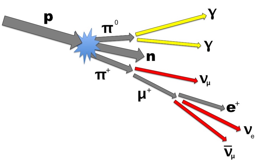
Figure 5: Illustration of the connection between gamma-rays and neutrinos, that are produced when the primary cosmic rays collide with some target around their source.

Ordinary astronomy and neutrinos:–

Then, there is one connection between neutrinos and photons that is in a sense obvious. We have explored the Universe with photons and we may suppose - even before any theoretical elaboration - that some of the known astronomical objects are also sources of high energy neutrinos. Here, we examine the opportunities offered by the observations of photons of different energies:
$\bullet$ a naive hypothesis concerns the highest $\gamma$-ray sources (up to some 10 TeV) that are currently known thanks to the Cherenkov telescopes (as HESS, Veritas, Magic, Milagro, etc). As we discuss hereafter, this applies mostly to galactic objects;
$\bullet$ when one considers the $\gamma$-ray sky as seen by the Fermi satellite below 100 GeV, the Milky Way is well distinguishable, but the main emission is from the rest of the sky, and it is dominated by the radiation emitted by the jets of the active galactic nuclei that point in our direction (blazars);
$\bullet$ ultraviolet and X-ray astronomy allows us to explore the active galactic nuclei, and in particular their cores or the surrounding regions, but also supernova remnants or compact stellar objects in the Galaxy;
$\bullet$ infrared astronomy allows us to see sites of intense stellar formation rich in dust, such as star-forming and/ or star-burst galaxies; likewise, it is possible to see CO and H molecular emission from the molecular clouds of the Milky Way: these object surely have one key ingredient for efficient neutrino radiation, namely, the target for cosmic ray collisions;
$\bullet$ the exploration of the sites of most energetic processes of the universe is helped by radio astronomy as well, even if it concerns photons of comparably low energy.

Connecting directly high-energy $\gamma$ and neutrinos:–

Let us consider the possibilities of a direct connection. High energy neutrinos above TeV are necessarily produced along with $\gamma$-rays of similar energies, but the contrary is not true. We can use the observed $\gamma$-rays to predict an upper bound for the neutrinos: in fact, $\gamma$-rays are produced also by electromagnetic mechanisms, and, in this case, a part of them is not associated with neutrinos. A direct connection requires two further conditions: on the $\gamma$-rays: 1) they are not reprocessed in the source and 2) they are not modified during the propagation. The first condition depends upon the source; it is true for supernova remnants and typically for galactic sources (except possibly for micro-quasars and perhaps for the galactic center), while for extragalactic sources this condition should be examined case by case. The condition on the propagation instead rests on the efficiency of the pair conversion reaction $\gamma+\gamma\to\mathrm{e}^{+}+\mathrm{e}^{-}$; the existence of the cosmic microwave background and of other photonic fields (especially the IR background, that is not precisely known) makes the universe opaque to $\gamma$-rays above 100 GeV and modifies also the galactic $\gamma$-rays with energies larger than a fraction of PeV. Thus, a direct connection between neutrinos above TeV and $\gamma$-rays is possible only for (some) galactic sources, while for extragalactic sources the links are indirect and an extrapolation in energy is required if we want to compare the $\gamma$-ray and the neutrino spectra. Considering this type of galactic sources, it was shown saak that we could receive a discernible signal in the neutrino telescopes only if the $\gamma$-ray flux is larger than

$$I_{\gamma}(>\mathrm{10\ TeV})=(1-2)\times 10^{-13}\,\mathrm{cm}^{-2}\,\mathrm{s}^{-1}$$ (A.1)

valid for few specific astrophysical sources. This draws a link with existing and future $\gamma$-ray telescopes.

References

- (1) J. Bahcall, Neutrino Astrophysics, Cambridge University Press (1989).
- (2) M. Fukugita and T. Yanagida, Physics of Neutrinos and Applications to Astrophysics, Springer (2003).
- (3) C. Giunti and C. W. Kim, Fundamentals of Neutrino Physics and Astrophysics, Oxford University Press (2009).
- (4) A. Capone, P. Lipari, F. Vissani, Neutrino Astronomy, in R. Aloisio, E. Coccia, F. Vissani, Multiple Messengers and Challenges in Astroparticle Physics, Springer (2018).
- (5) F. Vissani, Neutrino Sources and Properties, PoS GSSI 14, 001 (2015) [arXiv:1412.8386].
- (6) A. Suzuki and M. Koshiba, History of neutrino telescope/astronomy, Exper. Astron. 25, 209 (2009).
- (7) T. Chiarusi, M. Spurio, High-Energy Astrophysics with Neutrino Telescopes, Eur. Phys. J. C65, 649 (2010).
- (8) A. Strumia, F. Vissani, Neutrino masses, mixings, and…, arXiv:hep-ph/0606054v3 (2010).
- (9) J. Perrin, Matière et lumière - Essai de synthèse de la mécanique chimique, Ann. Phys. 9, 5 (1919).
- (10) J. Bahcall, Beta Decay in Stellar Interiors, Phys. Rev. 126, pp. 1143–1149 (1962).
- (11) J. Bahcall, Neutrinos from the Sun, Scientific American 221, No. 1, pp. 28-37 (1969).
- (12) B. T. Cleveland, T. Daily, R. Davis Jr., J. R. Distel, K. Lande, C. K. Lee, P. S. Wildenhain, J. Ullman, Measurement of the Solar Electron Neutrino Flux with the Homestake Chlorine Detector, APJ 496, Nr. 1, 505 (1998).
- (13) N. Vinyoles et al., A New Generation of Standard Solar Models, APJ 835 202 (2017).
- (14) The Borexino Collaboration, Final results of Borexino Phase-I on low-energy solar neutrino spectroscopy, Phys. Rev. D 89 112007 (2014).
- (15) F. L. Villante et al., A step toward CNO solar neutrino detection in liquid scintillators, Physics Letters B 701 3, pp. 336–341 (2011).
- (16) F. Vissani, Comparative analysis of SN1987A antineutrino fluence, J. Phys. G 42, 013001 (2015).
- (17) M. Ikeda et al. [Super-Kamiokande Collaboration], Search for Supernova Neutrino Bursts at Super-Kamiokande, Astrophys. J. 669 519 (2007).
- (18) V. S. Berezinskii, S. V. Bulanov, V. A. Dogiel, V. L. Ginzburg (Ed.), V. S. Ptuskin, Astrophysics of Cosmic Rays, North-Holland, Amsterdam (1990).
- (19) M. Spurio, Particles and Astrophysics - A Multi-Messenger Approach, Springer (2015).
- (20) T. K. Gaisser, R. Engel and E. Resconi, Cosmic Rays and Particle Physics, Cambridge University Press (2016).
- (21) F. Halzen, D. Hooper, High-energy neutrino astronomy: The Cosmic ray connection, Rept. Prog. Phys. 65, 1025 (2002)
- (22) F.W. Stecker, Cosmic Physics: The High Energy Frontier, J. Phys. G29, R47 (2003)
- (23) E. Waxman, Neutrino astrophysics: A new tool for exploring the universe, Science 315, 63 (2007)
- (24) P. Lipari, Proton and Neutrino Extragalactic Astronomy, Phys. Rev. D78, 083011 (2008)
- (25) T. DeYoung, Neutrino Astronomy with IceCube, Mod. Phys. Lett. A24, 1543 (2009)
- (26) L. A. Anchordoqui, T. Montaruli, In Search for Extraterrestrial High Energy Neutrinos, Ann. Rev. Nucl. Part. Sci. 60, 129 (2010)
- (27) U. F. Katz, C. Spiering, High-Energy Neutrino Astrophysics: Status and Perspectives, Prog. Part. Nucl. Phys. 67, 651 (2012)
- (28) G. Matthiae, The cosmic ray energy spectrum as measured using the Pierre Auger Observatory, New Journal of Physics 12 (2010).
- (29) C. Spiering, Towards High-Energy Neutrino Astronomy. A Historical Review, Eur. Phys. J. H 37 515 (2012).
- (30) G. Fantini, A. Gallo Rosso, F. Vissani and V. Zema, The formalism of neutrino oscillations: an introduction, in A. Ereditato, “The State of Art of Neutrino Physics,” World Scientific (2018) [arXiv:1802.05781].
- (31) F. Vissani, F. Aharonian and N. Sahakyan, On the Detectability of High-Energy Galactic Neutrino Sources, Astropart. Phys. 34, 778 (2011).