FFLO Superconductivity Mediated by Excitonic Fluctuation
in Semimetallic Ta2NiSe5
Abstract
We investigate the excitonic fluctuation and its mediated superconductivity in the quasi one-dimensional three-chain Hubbard model for Ta2NiSe5 known as a candidate material for the excitonic insulator. In the semiconducting case and the semimetallic case with a small band-overlapping where one conduction () band and one valence () band cross the Fermi level, the excitonic fluctuation with is enhanced due to the - Coulomb interaction and diverges towards the uniform excitonic order corresponding to the excitonic insulator. On the other hands, in the semimetallic case with a large band-overlapping where two bands and one band cross the Fermi level, the non-uniform excitonic fluctuation with corresponding to the nesting vector between the and Fermi-surfaces (FSs) becomes dominant and results in the Fulde-Ferrell-Larkin-Ovchinnikov (FFLO) excitonic order characterized by the condensation of excitons with finite center-of-mass momentum . Near the instability, the largely enhanced excitonic fluctuations mediate the - interband Cooper pairs with finite center-of-mass momentum resulting in the FFLO superconductivity, which is expected to be realized in the semimetallic Ta2NiSe5 under high pressure.
1 Introduction
Excitonic condensation in the electron-hole (e-h) system has been a central issue in the condensed matter physics since about six decades ago[1, 2, 3], where conduction electrons and valence holes can form bound states, and they spontaneously drive the system into the low-temperature ground state, called the excitonic phase (EP) or excitonic insulator (EI). Recent discoveries of new candidate materials gather a growing interest of EP in the real materials in terms of the emergence of the BCS-Bose-Einstein condensation (BEC) crossover [4, 5, 6, 7, 8, 9].
Recently, the ternary chalcogenide Ta2NiSe5 has received renewed attention as a strong candidate for the EI. The resistivity indicates a narrow gap semiconductor with a quasi one-dimensional (1-D) structure where a Ni chain and adjacent two Ta chains construct the 1-D three chain[10, 11]. A second-order structural transition from the orthorhombic to monoclinic phase occurs at a critical temperature =328 K[11], below which a remarkable flattening of the valence band top is observed in the angular resolved photo emission spectroscopy (ARPES) experiments[12, 13] without any sign of the magnetic and density-wave-type order.
Several theoretical studies have revealed that the transition is well accounted for by the excitonic condensation from a normal semiconductor (orthorhombic) to the EI (monoclinic) from a mean-field (MF) analysis for the 1-D three-chain Hubbard model[14, 15] and from a variational cluster approximation for the extended Falicov-Kimball model[16]. Recent optical measurements are also consistent with the EI phase below [17, 18] and is analyzed by the band structure calculation together with the density-matrix renormalization group study, exhibiting the strong coupling EI with the BEC of the exciton-pairs.[19]
When the pressure is applied for Ta2NiSe5[20, 21], is suppressed and the system changes from semiconducting to semimetallic both above and below , and then, finally becomes zero at a critical pressure GPa, around which the superconductivity is observed. Then, we have recently investigated the 1-D three-chain Hubbard model also in the semimetallic case and have found that the difference of the band degeneracy, the two-fold degenerate conduction bands and the nondegenerate valence band, inevitably causes the imbalance of each Fermi wavenumber and results in a remarkable excitonic state characterized by the condensation of excitons with finite center-of-mass (COM) momentum , the so-called Fulde-Ferrell-Larkin-Ovchinnikov (FFLO) excitonic state[22, 23], as previously discussed in the electron-hole bilayer systems with density imbalance[24, 25, 26]. More recently, a realistic quasi 1-D three-chain Hubbard model[27] has also been studied and a detailed excitonic phase diagram including the FFLO state has been obtained[28].
As the superconductivity is observed near the excitonic phase in Ta2NiSe5, the excitonic fluctuation is considered to be a key ingredient for the pairing mechanism as early discussed by Little for quasi 1-D organic superconductors[29] but has not been discussed for Ta2NiSe5 so far. The purpose of this paper is to investigate the enhancement of the excitonic fluctuations in quasi 1-D semimmetallic situation and superconductivity mediated by such the excitonic fluctuations in Ta2NiSe5 on the basis of the quasi 1-D three-chain Hubbard model where the FFLO excitonic order is found to take place in the semimetallic case[28].
This paper is organized as follows: In Sec. 2, we introduce a model Hamiltonian and give the formulation of the random phase approximation (RPA) and Eliashberg equation for the present model. Next in Sec. 3, we show the results for the normal-excitonic phase boundary diagram and the enhancement of the excitonic fluctuation and its effect on the superconductivity. In Sec. 4 we give the summary and discussion about the present mechanism and experimental prediction.
2 Model & Formulation
2.1 Hamiltonian

The quasi 1-D three-chain Hubbard model for Ta2NiSe5[15, 28] is schematically shown in Fig. 1 (a), where a Ni () chain and adjacent two Ta () chains construct the 1-D three chains[14], and these chains are weakly coupled with the neighboring three chains, which is explicitly given by the Hamiltonian,
| (1) | ||||
| (2) | ||||
| (6) | ||||
| (7) |
where and , are the annihilation operators for the , electrons with wavevector (unit cell at with unit lattice vectors and ), spin and chain index for the electron . , are the number operators and is a chemical potential. The matrix elements of are given by,
| (8) | |||
| (9) | |||
| (10) |
where the intra-chain hopping parameters, and , and the additional inter-chain hopping parameters, , and , are set to eV, eV, eV, eV, and eV, which are the same with the values of the previous study.[28] The resulting conduction bonding (anti-bonding) band,
| (11) |
and the valence band are plotted in Fig. 1 (b). is the band-overlap or band-gap where the and bands meet just at when eV) which gives the boundary between the semiconducting () and semimetallic () regime. As is considered to be a decreasing function of pressure, we vary as a parameter to examine the pressure effect on this model from semiconducting to semimetallic regime. In fact, we have estimated the band-overlap from the first-principles band calculation under pressure and have found that increases with increasing the pressure although the available lattice parameters under the pressure are restricted[17] and is difficult to obtain the explicit pressure dependence of .
In Eq. (1), we consider the intersite - Coulomb interaction which is crucial for the excitonic order and its fluctuation as shown below, while we neglect the on-site Coulomb interaction which can be effectively included in and/or the chemical potential within the MF approximation by excluding the magnetic and density-wave-type orders[14, 15, 22, 23, 27, 28]. In fact, such orders have not been observed experimentally in Ta2NiSe5.
2.2 Random Phase Approximation
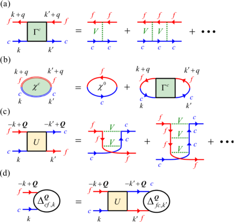
Here we employ the RPA which can describe the enhancement of the fluctuations around the MF critical point of the excitonic ordered phase recently obtained in the our previous work[28]. Within the RPA, the effect of the excitonic fluctuation is described by a summation of the ladder diagrams with respect to for the charge-orbital vertex as shown in Fig. 2 (a) which is given by the matrix representation as,
| (12) | ||||
| (13) | ||||
| (14) |
where and are the particle-hole bare susceptibility and the Green’s function ( matrix) with , and the momentum , and the fermionic and bosonic Matsubara frequencies , , respectively. is the site-orbital channels =1,2,3 (=) and is the unit matrix in the site-orbital basis.
The charge-orbital bare vertex due to the intersite Coulomb is
| (17) |
where we neglect the magnetic and density-wave-type fluctuations due to the effect of together with the ring diagrams with respect to since the same reason mentioned in the previous subsection. We also discuss the possibility of such the density, hybridization, and pair-formation-type condensation within the MF approximation for the intersite - Coulomb interaction in the present three-chain model in Appendix A.
In order to take the effect of the inter-cell - Coulomb interaction in the susceptibility, we transform and in Eq. (12) into the matrix representations and with , respectively,
| (18) | |||
| (19) |
where is the extended basis function similar to the three band - model for high- cuprate[30]and the explicit form is given in Appendix B. Then we obtain the charge-orbital susceptibility as shown in Fig. 2 (b),
| (20) | |||
| (21) | |||
| (22) |
where and , and
| (23) |
When the largest eigenvalue of reaches unity, the charge-orbital instability including the excitonic one with the ordering momentum takes place. The more explicit formulation of the phase boundary condition within the MF approximation for the excitonic phase order is given in Appendix C.
2.3 Linearized Eliashberg equation & Effective pairing interaction
In order to examine the superconductivity in the - density imbalanced systems, we solve the linearized Eliashberg equation with including the FFLO solution shown in Fig. 2 (d) which is given by
| (24) |
where is the superconducting (SC) gap function with the COM momentum of Cooper pairs . is the matrix representation of the effective pairing interaction for the spin-singlet state mediated by the charge-orbital (excitonic) fluctuation diagrammatically shown in Fig. 2 (c) and explicitly given by
| (25) |
which yields a large attractive interaction for near the charge-orbital instability with almost independent of . Eq. (24) is solved to obtain the gap function with the eigenvalue which becomes unity at the SC transition temperature .
Throughout the paper, the chemical potential is set so as to keep the electron number per unit cell: for any given band-overlap which corresponds to the situation of the semiconducting and semimetallic cases in Ta2NiSe5. The RPA and SC calculations are performed with 102416 -point meshes and 2048 Matsubara frequencies and eV as a realistic value of the case with weak screening. Here and hereafter, we measure the energy in units of eV.
3 Results
Here we focus only on the phase boundary owing to consider the excitonic fluctuation and the superconductivity and thus we set aside the electronic states below which is precisely studied in Ref.[28]
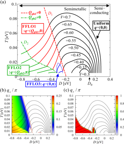
First we show the normal-excitonic phase (EP) transition temperature within the RPA as functions of as shown in Fig. 3 (a) where we search the maximum value of the bare excitonic susceptibility (= and determine the condition = for any given together with the COM momentum , which yields the critical values of [See Appendix C]. As well as the previous 1-D model study[22, 23], the dome-like structure of between semiconducting and semimetallic region is obtained depending on and , which originates from the van-Hove singularity of the density of states (DOS) in the present quasi 1-D nature together with the thermal effect on the excitonic susceptibility which explicitly includes the Fermi distribution function and satisfies the condition at finite [See Appendix C]. In contrast to the 1-D study[22, 23], the system enters into four distinct EPs; a conventional uniform EP with zero COM wavevector , and three FFLO EPs, FFLO1, FFLO2 and FFLO3 with finite as plotted in color maps of [Fig. 3 (b)] and [Fig. 3 (c)] on the - phase diagrams.
The uniform EP is stabilized over and with a small , and in particular below , the system becomes the semimetallic with a single -band and single -band crossing the Fermi level where the conventional (uniform) exciton condensation is achieved. On the other hands, with decreasing below where a new Fermi-surface (FS) of the -band emerges, the - density imbalance is inevitably induced as well as the e-h bilayer systems[24, 25, 26]. In such the situation, the FFLO1 exicitonic fluctuation given by the maximum of with the nesting wavevector between -and -bands, “- band nesting” , becomes more dominant than that of uniform one. Furthermore with decreasing and , a new FFLO fluctuation FFLO2 with the “- band nesting” wavevector dominates over the FFLO1 around . A third fluctuation FFLO3 with [] is also observed in lower between the two FFLO fluctuations. As discussed in the MF study[28], The weak -dependent peak structure of along is the origin of the present several FFLO phases as explicitly shown in Appendix E.
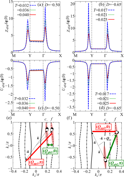
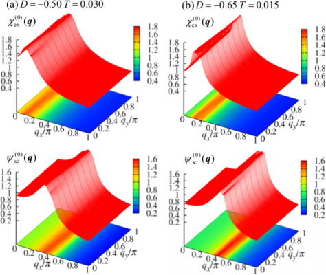
Figures 4 (a) and (b) show the static charge-orbital susceptibility with corresponding to the excitonic fluctuation at several temperatures for and . There are two sharp peaks at and corresponding to the particle-hole nesting vectors between the and FSs and the and FSs as shown in Figs. 4 (e) and (f), respectively, where the former (latter) peak dominates over the latter (former) one for (). When decreases, increases and finally diverges with () for () at a critical temperature below which the FFLO1 (FFLO2) excitonic order with the finite COM momentum of excitons () takes place as previously shown in our previous paper on the basis of the MF analysis[28].
When approaches , the effective pairing interaction between the and electrons with is largely enhanced for and due to the largely enhanced excitonic fluctuation mentioned above, and then mediates the - pairing with the gap function . The explicit results of the pairing interactions with = and are plotted in Fig. 4 (c) and (d) as the same plot of the corresponding as shown in Fig. 4 (a) and (b), where is largely developed with the corresponding wavevector and as a attractive pairing interaction between .
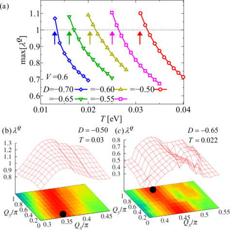
In Fig. 5 (a), we plot the -dependence of the eigenvalue of the Eliashberg equation Eq. (24) for several values of , where we set the value of for which becomes maximum. Systematic calculations of for various reveal that, for and (, and ), becomes maximum at () as shown in Fig. 5 (b) ((c)) and reaches unity at where the second-order phase transition for the FFLO SC state with the finite COM momentum of Cooper pairs () takes place. Therefore the enhancement of the FFLO excitonic fluctuations help the increase of through the strong enhancement of pairing interaction yielding finite the FFLO Cooper-pairs.
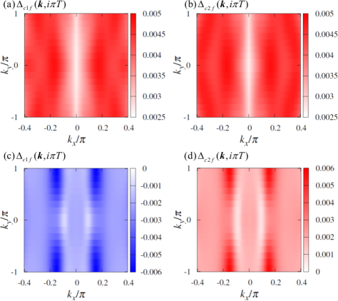
Here, we discuss the pairing mechanism of the FFLO SC state in the present system. In the case with , the bare SC susceptibility becomes maximum at due to the particle-particle nesting between the and FSs as shown in Fig. 4 (e). This SC fluctuation is largely enhanced by the pair scattering from to due to the effective pairing potential which has a large positive value for and divergently increases when approaching , resulting in the FFLO SC state of the pair with the COM momentum . As for the case with , the bare SC susceptibility becomes maximum at due to the particle-particle nesting between the and FSs (see Fig. 4 (f)) and is largely enhanced by the pair scattering from to due to which is large positive for , resulting in the FFLO SC state of the pair with the COM momentum . Actually, the obtained gap functions with and pairs have the same (opposite) sign for () as shown in Figs. 6 (a) and (b) ((c) and (d)), where the band representation of the gap function becomes dominant for () pair with bonding (anti-bonding) .
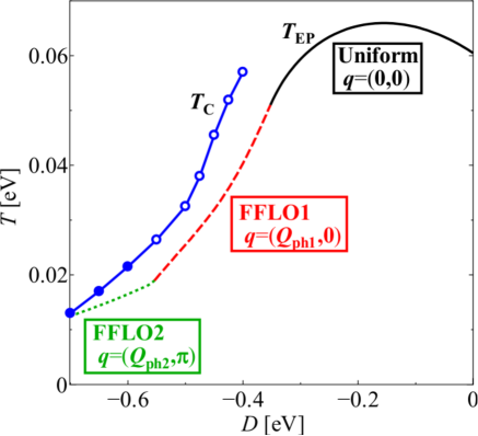
Finally, we summarize the transition temperatures of and as a function of in Fig. 7. When decreases, the excitonic susceptibilities with , and (see Fig. 4) diverge at the critical temperature below which the uniform, FFLO1 and FFLO2 EPs are realized[28] for , and , respectively. When approaching , the excitonic fluctuations are largely enhanced and mediate the FFLO superconductivity with near the FFLO1 EP and that with near the FFLO2 EP. Such the FFLO nesting mechanism can be possible for the high-pressured semimetallic situation of Ta2NiSe5 which is discussed in the following section. On the other hand in the semiconducting region with , the uniform excitonic fluctuation might mediate the uniform but strong-coupling pairing resulting in the BEC-type superconductivity which requires a strong-coupling theory beyond the present RPA approach.
4 Summary and Discussion
In summary, we have studied the quasi 1-D three-chain Hubbard model for Ta2NiSe5 within the RPA and have found that the FFLO superconductivity is mediated by the FFLO excitonic fluctuation which is largely enhanced towards the FFLO excitonic order realized in the semimetallic case with the imbalanced two and one FSs. The obtained FFLO superconductivity together with the FFLO excitonic order is expected to take place in the semimetallic Ta2NiSe5 under high pressure.
In this paper, we concentrate ourselves on the excitonic fluctuations and their SC mechanism within the MF-RPA theory in the semimetallic regime with the high-pressure and low temperature region where the BCS weak coupling treatment of the exciton-pairs and Cooper-pairs is justified. Hence the strong coupling theory like the dynamical mean-field theory is needed for the semiconducting regime with the ambient (low-pressure) and high temperature region where actually discussed by the experiments[31, 32] and theoretical calculations[16, 19]. Recently, we have also studied the same model with finite and on the basis of the dynamical mean-field theory (DMFT) and have found that the excitonic fluctuation dominates over the other fluctuations due to the strong enhancement of the local excitonic fluctuation and then yields the psedogap-like behavior in the conduction band dispersion. Explicit results with the DMFT together with the results of the strong-coupling pairing in the BEC regime will be presented in the near future.
Clear differences between the uniform, FFLO1 and FFLO2 excitonic phases obtained in this study are the ordered wavevectors =, and , respectively. Hence, by checking such the conduction-valence band nesting with the corresponding wavevectors, those excitonic states can be distinguished. Direct observation of the band dispersion by the ARPES experiment is one way to confirm the types of excitonic phases. We have already shown that the band dispersion in the FFLO phase becomes semimetallic both the FF[22] and LO states[28] in contrast to that in the uniform one which becomes fully gapped semiconducting and then we expect that the transport properties of the FFLO phases are different from those in the uniform phase. In addition, the non-trivial phase of the complex order parameters obtained in the FFLO states[28] is considered to be responsible for a kind of anomaly in the hole conductivity. Moreover, the optical response such as the resonant inelastic X-ray scattering[33] can become a good probe for detecting the enhancement of the excitonic dispersion when the exciton condensation occurs in the strong coupling regime. The significant softening of the particle-hole excitation with the wavevectors =, and would be observed towards each instability for the uniform, FFLO1 and FFLO2 phases, respectively.
For the realization of the present FFLO mechanism in actual system, it is essential that two conduction FSs exist in the high-pressure electronic states of Ta2NiSe5 as mentioned in Sec. 3, and in particular the number of -band FS in the high-pressure region around is still unsettled. In addition, the impurity effect on the EPs could rapidly decreases as studied by Zittartz[34] where the excitonic phase is easily destroyed and could rapidly decreases by the nonmagnetic impurity as same as the magnetic impurity effect on the conventional superconductivity. Therefore there are two possible FFLO SC scenarios under the assumption that is ; One is the FFLO1 scenario where the disorder is strong enough to suppress with relatively small corresponding to the FFLO1 region, while the other is the FFLO2 scenario where the disorder is relatively weak and survives in the FFLO1 region but disappears around the large- FFLO2 region. Which scenarios realize in the real material will depend on the strength of the disorder and such the study is an important future work.
The effect of the uniform monoclinic distortion[14, 15] would be still relevant for the high-pressured low-temperature phase[20, 21]. We check this effect in the present theory by adding a - hopping , and confirm that the enhancement of the FFLO excitonic fluctuation is almost unchanged but the uniform fluctuation is slightly suppressed. Furthermore, in our previous MF study on the same model[28], the coexisted excitonic state with the uniform () and FFLO () wavevector is stabilized against the both single- state of the uniform and FFLO state which is interesting in analogy with the multi- phase of the FFLO superconductivity[35].
The relation between the excitonic order and the uniform distortion including the phonon coupling together with the formation of the antiferroelectric and the ferroelectric toroidal moments, which is recently observed [36], is also important topic and should be clarified by the more microscopic analysis based on the effective Wannier-orbital model for the distorted low-temperature phase of Ta2NiSe5, and such the study is now under the way.
The authors give a special thanks to prof. Hidetoshi Fukuyama for providing interesting idea and variable comments and discussions. This research was supported in part by Multidisciplinary Cooperative Research Program in CCS, University of Tsukuba. This work was partially supported by a Grant-in-Aid for Scientific Research from the Ministry of Education, Culture, Sports, Science and Technology.
References
- [1] R. Knox: in“Solid State Physics”, ed. F. Seitz and D. Turnbull (Academic Press, New York, 1963), Suppl. 5, p. 1.
- [2] D. Jrome, T. M. Rice, and W. Kohn: Phys. Rev 158 (1967) 462.
- [3] B. I. Halperin and T. M. Rice: Rev. Mod. Phys 40 (1968) 755.
- [4] F. X. Bronold and H. Fehske: Phys. Rev. B 74 (2006) 165107.
- [5] D. Ihle, M. Pfafferott, E. Burovski, F. X. Bronold, and H. Fehske: Phys. Rev. B 78 (2008) 193103.
- [6] V.-N. Phan, K. W. Becker, and H. Fehske: Phys. Rev. B 81 (2010) 205117.
- [7] K. Seki, R. Eder, and Y. Ohta: Phys. Rev. B 84 (2011) 245106.
- [8] B. Zenker, D. Ihle, F. X. Bronold, and H. Fehske: Phys. Rev. B 85 (2012) 121102.
- [9] J. Kune: J. Phys.: Condens. Matter 27 (2015) 333201.
- [10] S. A. Sunshine and J. A. Ibers: Inorg. Chem. 24 (1985) 3611.
- [11] F. J. DiSalvo, C. H. Chen, R. M. Fleming, J. V. Waszczak, R. G. Dunn, S. A. Sunshine, and J. A. Ibers: J. Less-Common Met. 116 (1986) 51.
- [12] Y. Wakisaka, T. Sudayama, K. Takubo, T. Mizokawa, M. Arita, H. Namatame, M. Taniguchi, N. Katayama, M. Nohara, and H. Takagi: Phys. Rev. Lett 103 (2009) 026402.
- [13] Y. Wakisaka, T. Sudayama, K. Takubo, T. Mizokawa, N. L. Saini, M. Arita, H. Namatame, M. Taniguchi, N. Katayama, M. Nohara, and H. Takagi: J. Supercond. Nov. Magn. 25 (2012) 1231.
- [14] T. Kaneko, T. Toriyama, T. Konishi, and Y. Ohta: Phys. Rev. B 87 (2013) 035121.
- [15] K. Sugimoto, T. Kaneko, and Y. Ohta: Phys. Rev. B 93 (2016) 041105(R).
- [16] K. Seki, Y. Wakisaka, T. Kaneko, T. Toriyama, T. Konishi, T. Sudayama, N. L. Saini, M. Arita, H. Namatame, M. Taniguchi, N. Katayama, M. Nohara, H. Takagi, T. Mizokawa, and Y. Ohta: Phys. Rev. B 90 (2014) 155116.
- [17] Y. F. Lu, H. Kono, T. I. Larkin, A. W. Rost, T. Takayama, A. V. Boris, B. Keimer, and H. Takagi: Nat. Commun. 8 (2017) 14408.
- [18] T. I. Larkin, A. N. Yaresko, D. Propper, K. A. Kikoin, Y. F. Lu, T. Takayama, Y.-L. Mathis, A. W. Rost, H. Takagi, B. Keimer, and A. V. Boris: Phys. Rev. B 95 (2017) 195144.
- [19] K. Sugimoto, S. Nishimoto, T. Kaneko, and Y. Ohta: Phys. Rev. Lett 120 (2018) 247602.
- [20] A. Nakano, K. Sugawara, S. Tamura, N. Katayama, K. Matsubayashi, T. Okada, Y. Uwatoko, K. Munakata, A. Nakao, H. Sagayama, R. Kumai, K. Sugimoto, N. Maejima, A. Machida, T. Watanukig, and H. Sawa: IUCrJ 5 (2018).
- [21] K. Matsubayashi, N. Katayama, R. Yamanaka, A. Hisada, T. Okada, A. Nakano, H. Sawa, K. Munakata, A. Nakao, T. Kaneko, T. Toriyama, T. Konishi, Y. Ohta, H. Okamura, T. Mizokawa, M. Nohara, H. Takagi, and U. Uwatoko: submitted (2018).
- [22] T. Yamada, K. Domon, and Y. Ōno: J. Phys. Soc. Jpn 85 (2016) 053703.
- [23] K. Domon, T. Yamada, and Y. Ōno: J. Phys. Soc. Jpn 85 (2016) 065005.
- [24] P. Pieri, D. Neilson, and G. C. Strinati: Phys. Rev. B 75 (2007) 113301.
- [25] K. Yamashita, K. Asano, and T. Ohashi: J. Phys. Soc. Jpn 79 (2009) 033001.
- [26] J.-X. Zhu and A. R. Bishop: Phys. Rev. B 81 (2010) 115329.
- [27] K. Sugimoto and Y. Ohta: Phys. Rev. B 94 (2016) 085111.
- [28] K. Domon, T. Yamada, and Y. Ōno: J. Phys. Soc. Jpn 87 (2018) 054701.
- [29] W. A. Little: Phys. Rev 134 (1964) A1416.
- [30] P. B. Littlewood, C. M. Varma, S. Schmitt-Rink, and E. Abrahams: Phys. Rev. B 39 (1989) 12371.
- [31] S. Mor, M. Herzog, J. Noack, N. Katayama, M. Nohara, H. Takagi, A. Trunschke, T. Mizokawa, C. Monney, and J. Sthler: Phys. Rev. B 97 (2018) 115154.
- [32] K. Okazaki, Y. Ogawa, T. Suzuki, T. Yamamoto, T. Someya, S. Michimae, M. Watanabe, Y. Lu, M. Nohara, H. Takagi, N. Katayama, H. Sawa, M. Fujisawa, T. Kanai, N. Ishii, J. Itatani, T. Mizokawa, and S. Shin: Nat. Commun. 9 (2018) 4322.
- [33] R.-P. Wang, A. Hariki, A. Sotnikov, F. Frati, J. Okamoto, H.-Y. Huang, A. Singh, D.-J. Huang, K. Tomiyasu, C.-H. Du, J. Kune, and F. M. F. de Groot: Phys. Rev. B 98 (2018) 035149.
- [34] J. Zittartz: Phys. Rev 164 (1967) 575.
- [35] H. Shimahara: J. Phys. Soc. Jpn 67 (1998) 736.
- [36] A. Nakano, T. Hasegawa, S. Tamura, N. Katayama, S. Tsutsui, and H. Sawa: Phys. Rev. B 98 (2018) 045139.
Appendix A Intersite - Coulomb interaction Hamiltonian & MF approximation
Here we summarize the expression of the intersite - Coulomb interaction in the present three-chain model which can be written by,
| (26) | ||||
| (27) |
where is the inter-unitcell vectors between Ta-Ni as and thus . Within the MF approximation, this Hamiltonian can be written with three distinct MF order parameters: (i) density-type, (ii) hybridization-type, and (iii) pair-formation-type as shown in the following subsections.
A.1 (i) Density-type MF
The density-type MF Hamiltonian and their order parameters and can be written by,
| (28) | |||
| (29) | |||
| (30) |
where and electron density operators are written as follows,
| (31) |
where their MF expectations , correspond to the order parameters for the - and -electron charge density wave (CDW) with their modulated wavevector or for the phase separation . In normal phase, they become zero except for corresponding to the total electron number per unitcell . As seen in the last term of Eq.(28), and become finite at the same time and thus the -CDW and -CDW orders occur simultaneously due to the - intersite Coulomb interaction .
A.2 (ii) Hybridization-type MF
Similarly, the hybridization-type MF Hamiltonian and the order parameters are given by,
| (32) | |||
| (33) | |||
| (34) |
where the finite expectation values of , indicate the intersite - bond formation and also correspond to a spontaneous phase transition towards the EP with the exciton-pairs COM wavevector since has no - direct hopping.
A.3 (iii) Pair-formation-type MF
Finally, the pair-formation-type MF Hamiltonian and the order parameters are given by,
| (35) | |||
| (36) | |||
| (37) |
where the expectation values of and become finite when SC state with the interband - Cooper-pairs formation with the COM wavenumber emerges.
For the semiconducting and semimetallic systems, -electron number is almost fully occupied, , while -electron number is nearly empty, , where - and -electron charge susceptibilities and is small in comparison with the excitonic susceptibilities and in Eq.(45). Hence we can neglect charge density type order for describing the weak coupling (BCS) semimetallic regime as discussed in the main text.
Appendix B Explicit form of extended basis function
The explicit form of the extended basis function is written as follows,
| (38) | ||||
| (39) | ||||
| (40) | ||||
| (41) |
where =1-9 corresponds to the intra-cell orbital sets and =10-13 the inter-cell - orbital sets as =, =, =, =.
Appendix C MF Phase boundary condition
In this Appendix, we give the formulation of the excitonic and superconducting phase boundary within the MF approximation for the intersite - Coulomb interaction in the quasi three-chain Hubbard model and we also shows the superconducting phase boundary in the - plane which can be obtained for the negative - Coulomb which corresponds to the attractive pairing interaction between and electrons effectively.
C.1 Bare Green’s functions & bare susceptibilities for the three-chain model
The bare Green’s functions for the present quasi 1-D three-chain model can be written as follows,
| (42) | |||
| (43) | |||
| (44) |
where , , and . The bare susceptibilities for particle-hole and particle-particle channels and are also written as follows,
| (45) | |||
| (46) |
where is the site-orbital index . Especially for the semiconducting and semimetallic situation like the present system, the - coupled terms with are exclusively important for the excitonic fluctuation,
| (47) | |||
| (48) |
where is Fermi distribution function . Both susceptibilities become quite large and/or diverge at low when the - nesting conditions are satisfied in the semimetallic situation.
C.2 Excitonic phase boundary
Here we derive the EP boundary condition within the MF approximation. For simplicity, we drop the spin-dependence of the order parameter in Eq.(34) as since there is no magnetic sign in the present semimetallic system. Hence the excitonic order parameter can be written as follows,
| (49) |
where is the - anomalous Green’s function and becomes finite (zero) in excitonic (normal) phase which can be written by the -representation as follows,
| (50) |
Around the EP boundary, and in Eq.(49) are self-consistently determined so as to satisfy the linearized Dyson-Gorkov equations given by,
| (51) | |||
| (52) |
where in the first line we use in the normal phase. In Eq.(52), the -dependence of is given by and the frequency dependence of is dropped within the MF approximation for the static intersite Coulomb interaction . Thus we can set the following form in general,
| (53) |
where is the complex order parameter between the -site and -site in the same (left neighboring) unitcell. By substituting Eq.(53) into Eq.(52) we can obtain the simultaneous linear equations for four order parameters,
| (62) | |||
| (63) |
where is the bare particle-hole susceptibilities like Eq.(45) which are explicitly given by,
| (64) | |||
| (65) | |||
| (66) | |||
| (67) | |||
| (68) |
where =.
Then we can obtain four eigenvalues of the particle-hole susceptibility matrix analytically by using Ferrari’s method for the quartic equation for any given , and . The maximum eigenvalue of corresponds to the bare excitonic susceptibility which yields the EP boundary condition . If we drop in Eq.(63), the condition for the previous purely 1-D model[22, 23] returns as .
C.3 SC phase boundary
Next we derive the SC phase boundary condition within the MF approximation in similar way of the EP case. Here we consider only the spin-singlet gap function in Eq.(37) as which is written by,
| (69) |
where is the - anomalous Green’s function for SC phase and becomes finite (zero) in superconducting (normal) phase which is given by the -representation as follows,
| (70) |
Around the SC phase boundary, and in Eq.(69) are self-consistently determined so as to satisfy the linearized Dyson-Gorkov equations which are given by,
| (71) | |||
| (72) |
where in the first line we use in the normal phase. In Eq.(72), the -dependence of is given by and the frequency dependence of is dropped for the same reason of the previous subsection. The explicit form of is applicable as the same form of ,
| (73) |
and thus we can obtain the similar equations with the EP case which is given by,
| (82) | |||
| (83) |
where is the bare particle-particle susceptibilities like Eq.(46) which are explicitly given by,
| (84) | |||
| (85) | |||
| (86) | |||
| (87) | |||
| (88) |
where =.
Then we can obtain four eigenvalues of the particle-particle susceptibility matrix analytically as the same as the EP case for any given , and . The maximum eigenvalue of corresponds to the bare SC susceptibility which yields the SC boundary condition , where the negative - interaction is needed because .
Appendix D SC phase boundary in - plane
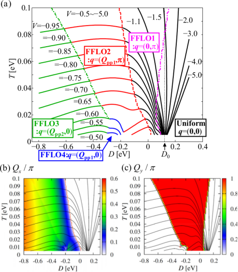
In Figure 8 (a), we show the SC phase boundaries with several values of in - plane as well as the EP case mentioned in the main text. Contrary to the EP case, five distinct SC phases are observed ; a conventional uniform SC state with , and four FFLO SC phases, FFLO1, FFLO2, FFLO3 and FFLO4 with finite as plotted in color maps of [Fig. 8 (b)] and [Fig. 8 (c)] as the same as the case of EP [Fig. 3 (b) and (c)].
A more complicated ()-dependence of is observed. emerges around the semiconducting-semimetalic boundary with any strength of , but its development direction is highly dependent on ; when is relatively small (weak and intermediate -regime), increases for while when is large (strong -regime), develops for .
For weak -regime , two domes of emerge as a function of around the shallow from and the relatively deep from . On the other hands, when reaches the intermediate -regime () the two domes combine into one and increases with increasing with exhibiting a weak -dependence for wide semimetallic region. Such the behavior can be understood by the BCS-formula of the transition temperature, , where is the energy cut-off and is the magnitude of the attraction and is the density of states on the FSs where is almost constant for in the semimetallic situation.
In such the weak and intermediate -regime with , the FFLO SC states with the COM wavevectors can be possible as well as the FFLO EP case but their wavevector differs from the exciton COM wavevector in the main text, where the Cooper-pairs here consist of -band electron with and -band electron with in contrast to the exciton-pairs between the -FS with and -FS with .
Firstly the FFLO1 SC state is realized for the shallow region where with becomes dominant due to the - band nesting effect. When the -FS emerges, the - density imbalance shrinks the -FS by sliding in -direction (not shown) so as to satisfy the particle-hole FS compensation which induces the - band nesting with finite corresponding to the FFLO2 SC states with as shown in Fig. 8 (a) and (b). The further decrease of gives rise to the change of the dominant from the - nesting with to the - nesting corresponding to the emergence of the FFLO3 SC as shown in Fig. 8 (a) and (b). A fourth fluctuation FFLO4 SC with is also observed in lower and small between the FFLO2 and FFLO3 SC fluctuations.
Furthermore for strong -regime , the semiconducting-SC transition for can occur only at high temperature as shown in Fig. 8 (a). In such the situation, become finite due to the thermal excitation and takes the maximum with corresponding to the instability towards the uniform SC states. However, is completely suppressed with decreasing and also becomes absolutely zero at in the absence of FSs.
Appendix E -dependence of bare susceptibilities of and
The present phase diagrams for normal-EP and normal-SC phase are attributed to the intrinsic - density imbalance of the present quasi 1-D property which yields two types of the - nesting effects between the - and - bands in the particle-hole (excitonic) and particle-particle (superconducting) susceptibilities and . In order to see such the quasi 1-D structure explicitly, we plot the -dependence of and in - plane for several values of and in Fig. 9 where (a) and (b) , respectively.
Both of and shows the clear quasi 1-D peak structures as a function of and their weak -dependences over the - compensated semimetallic region with three-FSs as shown upper and lower lines of Fig. 9, respectively. With decreasing and , the both giving the peak of and increase, where of corresponds to the EP instabilities towards from FFLO1 EP to FFLO2 EP and of corresponds to the SC phase instabilities towards from FFLO2 SC phase to FFLO3 SC phase. Such the various structures of and in - plane is attributed to the newly-added inter-chain hoppings which yields the different curvature of FSs between and -bands.