Multiple impurities and combined local density approximations in Site-Occupation Embedding Theory

Abstract

Site-occupation embedding theory (SOET) is an in-principle-exact multi-determinantal extension of density-functional theory for model Hamiltonians. Various extensions of recent developments in SOET [Senjean et al., Phys. Rev. B 97, 235105 (2018)] are explored in this work. An important step forward is the generalization of the theory to multiple impurity sites. We also propose a new single-impurity density-functional approximation (DFA) where the density-functional impurity correlation energy of the two-level (2L) Hubbard system is combined with the Bethe ansatz local density approximation (BALDA) to the full correlation energy of the (infinite) Hubbard model. In order to test the new DFAs, the impurity-interacting wavefunction has been computed self-consistently with the density matrix renormalization group method (DMRG). Double occupation and per-site energy expressions have been derived and implemented in the one-dimensional case. A detailed analysis of the results is presented, with a particular focus on the errors induced either by the energy functionals solely or by the self-consistently converged densities. Among all the DFAs (including those previously proposed), the combined 2L-BALDA is the one that performs the best in all correlation and density regimes. Finally, extensions in new directions, like a partition-DFT-type reformulation of SOET, a projection-based SOET approach, or the combination of SOET with Green functions, are briefly discussed as a perspective.

I Introduction

The accurate and low-cost description of strongly correlated materials remains one of the most challenging task in electronic structure theory As highly accurate wavefunction-based methods are too expensive to be applied to the whole system of interest, simplified and faster solutions have to be considered. Such simplications should ideally not alter the description of strong correlation effects. This is where the challenge stands. Based on the cogent argument that strong electron correlation is essentially local Pulay (1983); Saebo and Pulay (1993); Hampel and Werner (1996) and that the region of interest is one part of a much larger (extended) system, embedding approaches are mainly used in practice Sun and Chan (2016). The basic idea is to map the fully-interacting problem onto a so-called impurity-interacting one. In the Hubbard model, the impurity corresponds to an atomic site. Among such embedding techniques are the well-established dynamical mean-field theory (DMFT) Georges and Kotliar (1992); Georges et al. (1996); Kotliar and Vollhardt (2004); Held (2007); Zgid and Chan (2011), its cluster  Hettler et al. (1998, 2000); Lichtenstein and Katsnelson (2000); Kotliar et al. (2001); Maier et al. (2005) and diagrammatic Rohringer et al. (2018) extensions, as well as combinations of DMFT with either density-functional theory (DFT) [the so-called DMFT+DFT approach Kotliar et al. (2006)] or the Green-function-based GW method  Sun and Kotliar (2002); Biermann et al. (2003); Karlsson (2005); Boehnke et al. (2016); Werner and Casula (2016); Nilsson et al. (2017). Such combinations aim at incorporating non-local correlation effects in DMFT. More recently, the self-energy embedding theory (SEET) Kananenka et al. (2015); Lan et al. (2015); Zgid and Gull (2017); Lan et al. (2017), which can be applied to both model and ab initio Hamiltonians, has been developed. Let us stress that all the aforementioned embedding techniques use the frequency-dependent one-particle Green function as basic variable.

Alternative frequency-independent approaches like the density-matrix embedding theory (DMET) Knizia and Chan (2012, 2013); Bulik et al. (2014); Zheng and Chan (2016); Wouters et al. (2016, 2017); Rubin (2016) have emerged in recent years. By construction, standard approximate DMET does not describe correlation effects in the environment, thus requiring the treatment of more than one impurity site in order to obtain reasonably accurate results Knizia and Chan (2012). More correlation can be incorporated into DMET by using an antisymmetrized geminal power wavefunction Tsuchimochi et al. (2015), or, alternatively, by improving the description of the boundary between the fragment and the bath Welborn et al. (2016). Note that Ayral et al. Ayral et al. (2017) succeeded recently in establishing formal connections between DMET, DMFT and the rotationally invariant slave bosons (RISB) theory Frésard and Wölfle (1992); Lechermann et al. (2007).

This paper deals with another frequency-independent approach, namely site-occupation embedding theory (SOET) Fromager (2015); Senjean et al. (2017, 2018). While, in conventional Kohn–Sham (KS) DFT, the fully-interacting problem is mapped onto a non-interacting one, an auxiliary impurity-interacting system is used in SOET for extracting the density (i.e. the site occupations in this context) and, through an appropriate density functional for the environment (referred to as bath), the total energy. From a quantum chemical point of view, SOET is nothing but a multi-determinantal extension of KS-DFT for model Hamiltonians Chayes et al. (1985); Gunnarsson and Schönhammer (1986); Capelle and Campo Jr. (2013). In a recent paper Senjean et al. (2018), the authors explained how exact expressions for the double occupation and the per-site energy of the uniform Hubbard model can be extracted from SOET. They also proposed various local density-functional approximations for the bath. The latter work suffered from two main weaknesses. First of all, the complete self-consistent formulation of the theory was done only for a single impurity site, thus preventing a gradual transition from KS-DFT (no impurity sites) to pure wavefunction theory (no bath sites). Moreover, none of the proposed DFAs gave satisfactory results in all correlation and density regimes.

We explain in this work how these limitations can be overcome. The paper is organized as follows. First, an in-principle-exact generalization of SOET to multiple impurity sites is derived in Sec. II.1. The resulting expressions for the double occupation and the per-site energy in the uniform case are given in Sec. II.2. Existing and newly proposed DFAs are then discussed in detail in Sec. III. Following the computational details in Sec. IV, results obtained at half-filling (Sec. V.1) and away from half-filling (Secs. V.2 and V.3) are presented and analyzed. Exact properties of the impurity correlation potential are discussed in Sec. V.4. Conclusions and perspectives are finally given in Sec. VI.

II Theory

II.1 Site-occupation embedding theory with multiple impurities

Let us consider the (not necessarily uniform) $L$-site Hubbard Hamiltonian with external potential $\mathbf{v}\equiv\{v_{i}\}_{0\leq i\leq L-1}$,

$$\hat{H}(\mathbf{v})=\hat{T}+\hat{U}+\hat{V}(\mathbf{v}).$$ (1)

The hopping operator, which is the analog for model Hamiltonians of the kinetic energy operator, reads as follows in second quantization,

$$\hat{T}=-t\sum_{\langle i,j\rangle}\sum_{\sigma=\uparrow,\downarrow}\hat{c}^{\dagger}_{i\sigma}\hat{c}_{j\sigma},$$ (2)

where $t>0$ is the so-called hopping parameter and $\langle i,j\rangle$ means that the atomic sites $i$ and $j$ are nearest neighbors. The on-site two-electron repulsion operator with strength $U$ and the local external potential operator (which is the analog for model Hamiltonians of the nuclear potential) are expressed in terms of the spin-density $\hat{n}_{i\sigma}=\hat{c}_{i\sigma}^{\dagger}\hat{c}_{i\sigma}$ and density $\hat{n}_{i}=\hat{n}_{i\uparrow}+\hat{n}_{i\downarrow}$ operators as follows,

$$\hat{U}=U\sum_{i}\hat{n}_{i\uparrow}\hat{n}_{i\downarrow},$$ (3)

and

$$\hat{V}(\mathbf{v}) = \sum_{i}v_{i}\hat{n}_{i},$$ (4)

respectively.

The exact ground-state energy $E(\mathbf{v})$ of $\hat{H}(\mathbf{v})$ can be obtained variationally as follows, in complete analogy with conventional DFT Hohenberg and Kohn (1964),

$$E(\mathbf{v})=\underset{\mathbf{n}}{\rm min}\left\{F(\mathbf{n})+(\mathbf{v}|\mathbf{n})\right\},$$ (5)

where $\mathbf{n}\equiv\{n_{i}\}_{0\leq i\leq L-1}$ is a trial collection of site occupations (simply called density in the following) and $(\mathbf{v}|\mathbf{n})=\sum_{i}v_{i}n_{i}$. Within the Levy–Lieb (LL) constrained-search formalism Levy (1979), the Hohenberg–Kohn functional can be rewritten as follows in this context,

$$F(\mathbf{n})=\underset{\Psi\rightarrow\mathbf{n}}{\rm min}\left\{\langle\Psi|\hat{T}+\hat{U}|\Psi\rangle\right\},$$ (6)

where the minimization is restricted to wavefunctions $\Psi$ with density $\mathbf{n}$. As shown in previous works Fromager (2015); Senjean et al. (2017, 2018), the exact minimizing density in Eq. (5) can be obtained from a fictitious partially-interacting system consisting of interacting impurity sites surrounded by non-interacting ones (the so-called bath sites), thus leading to an in-principle-exact SOET. While our recent developments focused on the single-impurity version of SOET, we propose in the following a general formulation of the theory with an arbitrary number of impurity sites. Such a formulation was briefly mentioned in Ref. Fromager (2015) for the purpose of deriving an adiabatic connection formula for the correlation energy of the bath.

Let us introduce the analog for $M$ impurity sites of the LL functional,

$$F_{M}^{{\rm imp}}(\mathbf{n})=\underset{\Psi\rightarrow\mathbf{n}}{\rm min}\left\{\left\langle\Psi\middle|\hat{T}+\hat{U}_{M}\middle|\Psi\right\rangle\right\},$$ (7)

where $\hat{U}_{M}=U\sum^{M-1}_{i=0}\hat{n}_{i\uparrow}\hat{n}_{i\downarrow}$. Note that, for convenience, the impurity sites have been labelled as $i=0,1,\ldots,M-1$. If we now introduce the complementary Hartree-exchange-correlation (Hxc) functional for the bath,

$$\overline{E}_{{\rm Hxc},M}^{\rm bath}(\mathbf{n}) = F(\mathbf{n})-F_{M}^{\rm imp}(\mathbf{n}),$$ (8)

the ground-state energy expression in Eq. (5) can be rewritten as follows,

$$E(\mathbf{v})=\underset{\mathbf{n}}{\rm min}\Bigg{\{} \underset{\Psi\rightarrow\mathbf{n}}{\rm min}\left\{\left\langle\Psi\middle|\hat{T}+\hat{U}_{M}\middle|\Psi\right\rangle\right\}$$ (9)

$$+\overline{E}_{{\rm Hxc},M}^{\rm bath}(\mathbf{n})+(\mathbf{v}|\mathbf{n})\Bigg{\}},$$

or, equivalently,

$$E(\mathbf{v})=\underset{\mathbf{n}}{\rm min}\Bigg{\{}\underset{\Psi\rightarrow\mathbf{n}}{\rm min}\Big{\{} \left\langle\Psi\middle|\hat{T}+\hat{U}_{M}\middle|\Psi\right\rangle$$ (10)

$$+\overline{E}_{{\rm Hxc},M}^{\rm bath}(\mathbf{n}^{\Psi})+(\mathbf{v}|\mathbf{n}^{\Psi})\Big{\}}\Bigg{\}},$$

where $\mathbf{n}^{\Psi}\equiv\left\{\langle\Psi|\hat{n}_{i}|\Psi\rangle\right\}_{0\leq i\leq L-1}$, thus leading to the final variational expression

$$E(\mathbf{v})=\underset{\Psi}{\rm min}\Big{\{} \left\langle\Psi\middle|\hat{T}+\hat{U}_{M}\middle|\Psi\right\rangle+\overline{E}_{{\rm Hxc},M}^{\rm bath}\left(\mathbf{n}^{\Psi}\right)+\left(\mathbf{v}|\mathbf{n}^{\Psi}\right)\Big{\}}.$$

The minimizing $M$-impurity-interacting wavefunction $\Psi_{M}^{\rm imp}$ in Eq. (II.1) reproduces the exact density profile of the fully-interacting system described by the Hubbard Hamiltonian in Eq. (1). From the stationarity in $\Psi_{M}^{\rm imp}$ of the energy, we obtain the following self-consistent equation,

$$\displaystyle\left(\hat{T}+\hat{U}_{M}+\displaystyle\sum_{i}v^{\rm emb}_{M,i}\,\hat{n}_{i}\right)|\Psi_{M}^{\rm imp}\rangle=\mathcal{E}_{M}^{\rm imp}|\Psi_{M}^{\rm imp}\rangle,$$ (12)

where

$$v^{\rm emb}_{M,i}=v_{i}+\dfrac{\partial\overline{E}^{\rm bath}_{{\rm Hxc},M}(\mathbf{n}^{\Psi_{M}^{\rm imp}})}{\partial n_{i}}$$ (13)

plays the role of an embedding potential for the $M$ impurities. In the particular case of a uniform half-filled density profile, the embedding potential equals zero in the bath and $-U/2$ on the impurity sites. This key result, which appears when applying the hole-particle symmetry transformation to the impurity-interacting LL functional, is proved in Appendix A, thus providing a generalization of Appendix C in Ref. Senjean et al. (2018). Note that the KS and Schrödinger equations are recovered from Eq. (12) when $M=0$ and $M=L$ (i.e. the total number of sites), respectively. In SOET, $M$ is in the range $0<M<L$, thus leading to a hybrid formalism where a many-body correlated wavefunction is embedded into a DFT potential. In practice, Eq. (12) can be solved, for example, by applying an exact diagonalization procedure Senjean et al. (2017) (which corresponds to a full configuration interaction) for small rings, or by using the more advanced density matrix renormalization group (DMRG) method which allows for the description of larger systems Senjean et al. (2018).

Let us now return to the expression in Eq. (8) of the complementary Hxc energy for the bath. By using the KS decompositions of the fully-interacting and $M$-impurity-interacting LL functionals,

$$F(\mathbf{n})=T_{\rm s}(\mathbf{n})+E_{\rm Hxc}(\mathbf{n})$$ (14)

and

$$F_{M}^{\rm imp}(\mathbf{n})=T_{\rm s}(\mathbf{n})+E^{\rm imp}_{{\rm Hxc},M}(\mathbf{n}),$$ (15)

respectively, where the non-interacting kinetic energy functional reads as follows in this context,

$$T_{\rm s}(\mathbf{n})=\underset{\Psi\rightarrow\mathbf{n}}{\rm min}\{\langle\Psi|\hat{T}|\Psi\rangle\},$$ (16)

we obtain

$$\overline{E}_{{\rm Hxc},M}^{\rm bath}(\mathbf{n})=E_{\rm Hxc}(\mathbf{n})-E^{\rm imp}_{{\rm Hxc},M}(\mathbf{n}).$$ (17)

If we now separate the Hxc energies into Hx (i.e. mean-field) and correlation contributions,

$$E_{\rm Hxc}(\mathbf{n}) = \dfrac{U}{4}\sum_{i}n_{i}^{2}+E_{\rm c}(\mathbf{n}),$$ (18)

and

$$E^{\rm imp}_{{\rm Hxc},M}(\mathbf{n}) = \dfrac{U}{4}\sum^{M-1}_{i=0}n_{i}^{2}+E^{\rm imp}_{{\rm c},M}(\mathbf{n}),$$ (19)

we obtain the final expression

$$\overline{E}_{{\rm Hxc},M}^{\rm bath}(\mathbf{n})=\dfrac{U}{4}\sum_{i\geqslant M}n_{i}^{2}+\overline{E}_{{\rm c},M}^{{\rm bath}}(\mathbf{n}),$$ (20)

where

$$\overline{E}_{{\rm c},M}^{\rm bath}(\mathbf{n})=E_{\rm c}(\mathbf{n})-E_{{\rm c},M}^{\rm imp}(\mathbf{n}).$$ (21)

While local density approximations (LDA) based, for example, on the Bethe ansatz (BALDA) are available for $E_{\rm c}(\mathbf{n})$ in the literature Lima et al. (2002, 2003); Capelle et al. (2003), no DFA has been developed so far for modeling the correlation energy of multiple impurity sites. Existing approximations for a single impurity are reviewed in Sec. III.2. Newly proposed DFAs will be introduced in Secs. III.3 and III.4.

II.2 Exact double occupation and per-site energy expressions in the uniform case

In this section we derive exact SOET expressions for the per-site energy and double occupancy in the particular case of the uniform Hubbard system ($\mathbf{v}=\mathbf{0}$) for which the LDA decomposition of the full correlation energy in terms of per-site contributions,

$$E_{\rm c}(\mathbf{n})=\sum_{i}e_{\rm c}(n_{i}),$$ (22)

is exact. Thus we extend to multiple impurities Eqs. (21) and (23) of Ref. Senjean et al. (2018).

For that purpose, let us introduce the following per-site analog of Eq. (21),

$$\overline{e}_{{\rm c},M}^{\rm bath}(\mathbf{n})=\dfrac{1}{M}\left[\left(\sum^{M-1}_{i=0}e_{c}(n_{i})\right)-E_{{\rm c},M}^{\rm imp}(\mathbf{n})\right],$$ (23)

which, for a uniform density profile $\underline{n}=(n,n,\ldots,n)$, gives

$$\overline{e}_{{\rm c},M}^{\rm bath}(\underline{n})=e_{c}(n)-\dfrac{E_{{\rm c},M}^{\rm imp}(\underline{n})}{M}.$$ (24)

Note that, when combining Eqs. (22) and (23) with Eq. (21), we obtain the following expression for the bath correlation energy,

$$\overline{E}_{{\rm c},M}^{\rm bath}(\mathbf{n})=\sum_{i\geqslant M}e_{\rm c}(n_{i})+M\overline{e}_{{\rm c},M}^{\rm bath}(\mathbf{n}).$$ (25)

By inserting the decomposition in Eq. (24) into the exact double site-occupation expression Capelle and Campo Jr. (2013) (we denote $E=E({\mathbf{v}=\mathbf{0}})$ for simplicity),

$$d=\langle\hat{n}_{i\uparrow}\hat{n}_{i\downarrow}\rangle=\dfrac{1}{L}\dfrac{\partial E}{\partial U}=\dfrac{n^{2}}{4}+\dfrac{\partial e_{\rm c}(n)}{\partial U},$$ (26)

where $n=N/L$ and $N$ is the total number of electrons, it comes from Eq. (19),

$$d=\dfrac{1}{M}\dfrac{\partial E_{{\rm Hxc},M}^{\rm imp}(\underline{n})}{\partial U}+\dfrac{\partial\overline{e}_{{\rm c},M}^{\rm bath}(\underline{n})}{\partial U}.$$ (27)

By using the fact that, in the particular (uniform) case considered here, $E=F(\underline{n})$ and, according to the Hellmann–Feynman theorem (see Eq. (II.1)),

$$\dfrac{\partial E}{\partial U}=\sum^{M-1}_{i=0}\langle\hat{n}_{i\uparrow}\hat{n}_{i\downarrow}\rangle_{\Psi_{M}^{\rm imp}}+\dfrac{\partial\overline{E}_{{\rm Hxc},M}^{\rm bath}(\underline{n})}{\partial U},$$ (28)

where

$$\left\langle\Psi_{M}^{\rm imp}\middle|\hat{n}_{i}\middle|\Psi_{M}^{\rm imp}\right\rangle=n$$ (29)

for any site $i$, it comes from the separations in Eqs. (8) and (15) that

$$\dfrac{\partial}{\partial U}\left[E-\overline{E}_{{\rm Hxc},M}^{\rm bath}(\underline{n})\right] = \sum^{M-1}_{i=0}\langle\hat{n}_{i\uparrow}\hat{n}_{i\downarrow}\rangle_{\Psi_{M}^{\rm imp}}$$ (30)

$$= \dfrac{\partial F_{M}^{\rm imp}(\underline{n})}{\partial U}$$

$$= \dfrac{\partial E_{{\rm Hxc},M}^{\rm imp}(\underline{n})}{\partial U}.$$

Finally, combining Eqs. (27), (29) and (30) leads to the following exact expression for the double occupation in SOET with multiple impurities,

$$d=\dfrac{1}{M}\sum^{M-1}_{i=0}\langle\hat{n}_{i\uparrow}\hat{n}_{i\downarrow}\rangle_{\Psi_{M}^{\rm imp}}+\dfrac{\partial\overline{e}_{{\rm c},M}^{\rm bath}({\bf n}^{\Psi_{M}^{\rm imp}})}{\partial U}.$$ (31)

The expression derived in Ref. Senjean et al. (2018) in the particular case of a single impurity site is recovered from Eq. (31) when $M=1$. Note also that the double occupations of the impurity sites are in principle not equal to each other in the fictitious $M$-impurity-interacting system, simply because translation symmetry is broken, as readily seen from Eq. (12), even though the embedding potential restores uniformity in the density profile.

Turning to the per-site energy Lima et al. (2003),

$$e=E/L=t_{\rm s}(n)+\dfrac{U}{4}n^{2}+e_{\rm c}(n),$$ (32)

where $t_{\rm s}(n)$ is the per-site non-interacting kinetic energy functional, we can insert Eq. (24) into Eq. (32) and use Eqs. (15) and (19), thus leading to

$$e=t_{\rm s}(n)+\dfrac{1}{M}\left(F_{M}^{\rm imp}(\underline{n})-T_{\rm s}(\underline{n})\right)+\overline{e}_{{\rm c},M}^{\rm bath}(\underline{n}).$$ (33)

Moreover, applying once more the Hellmann–Feynman theorem to the variational energy expression in Eq. (II.1) gives

$$t\dfrac{\partial E}{\partial t}=\left\langle\Psi_{M}^{\rm imp}\middle|\hat{T}\middle|\Psi_{M}^{\rm imp}\right\rangle+t\dfrac{\partial\overline{E}_{{\rm Hxc},M}^{\rm bath}(\underline{n})}{\partial t},$$ (34)

or, equivalently,

$$\left\langle\Psi_{M}^{\rm imp}\middle|\hat{T}\middle|\Psi_{M}^{\rm imp}\right\rangle=t\dfrac{\partial F_{M}^{\rm imp}(\underline{n})}{\partial t},$$ (35)

which, for $U=0$, leads to

$$T_{\rm s}(\underline{n})=t\dfrac{\partial T_{\rm s}(\underline{n})}{\partial t}.$$ (36)

As a result, the second term in the right-hand side of Eq. (33) can be simplified as follows,

$$F_{M}^{\rm imp}(\underline{n})-T_{\rm s}(\underline{n})=\left\langle\Psi_{M}^{\rm imp}\middle|\hat{T}\middle|\Psi_{M}^{\rm imp}\right\rangle-T_{\rm s}(\underline{n})$$

$$+U\sum^{M-1}_{i=0}\langle\hat{n}_{i\uparrow}\hat{n}_{i\downarrow}\rangle_{\Psi_{M}^{\rm imp}}$$

$$=t\dfrac{\partial{E}_{{\rm c},M}^{\rm imp}(\underline{n})}{\partial t}+U\sum^{M-1}_{i=0}\langle\hat{n}_{i\uparrow}\hat{n}_{i\downarrow}\rangle_{\Psi_{M}^{\rm imp}},$$ (37)

thus leading, according to Eq. (24), to the final exact per-site energy expression,

$$e = t_{\rm s}(n)+\dfrac{U}{M}\sum^{M-1}_{i=0}\langle\hat{n}_{i\uparrow}\hat{n}_{i\downarrow}\rangle_{\Psi_{M}^{\rm imp}}+t\dfrac{\partial e_{\rm c}(n)}{\partial t}$$ (38)

$$-t\dfrac{\partial\overline{e}_{{\rm c},M}^{\rm bath}(\underline{n})}{\partial t}+\overline{e}_{{\rm c},M}^{\rm bath}(\underline{n}),$$

or, equivalently,

$$e = \dfrac{1}{M}\left.\sum^{M-1}_{i=0}\left[t_{\rm s}(n_{i}^{\Psi})+t\dfrac{\partial e_{\rm c}(n_{i}^{\Psi})}{\partial t}+{U}\langle\hat{n}_{i\uparrow}\hat{n}_{i\downarrow}\rangle_{\Psi}\right]\right|_{\Psi=\Psi_{M}^{\rm imp}}$$ (39)

$$+\left.\left[\overline{e}_{{\rm c},M}^{\rm bath}({\bf n}^{\Psi})-t\dfrac{\partial\overline{e}_{{\rm c},M}^{\rm bath}({\bf n}^{\Psi})}{\partial t}\right]\right|_{\Psi={\Psi_{M}^{\rm imp}}}.$$

Note that the expression in Eq. (39), which is a generalization for multiple impurities of the energy expression derived in Ref. Senjean et al. (2018), is convenient for practical (approximate) SOET calculations where the density profile calculated self-consistently might deviate significantly from uniformity Senjean et al. (2018). Finally, as shown in Appendix B, since the exact per-site bath correlation functional fulfills the fundamental relation,

$$\overline{e}_{{\rm c},M}^{\rm bath}({\bf n}) = t\dfrac{\partial\overline{e}_{{\rm c},M}^{\rm bath}({\bf n})}{\partial t}+{U}\dfrac{\partial\overline{e}_{{\rm c},M}^{\rm bath}({\bf n})}{\partial U},$$ (40)

Eq. (39) can be further simplified as follows,

$$e = \dfrac{1}{M}\left.\sum^{M-1}_{i=0}\left[t_{\rm s}(n_{i}^{\Psi})+t\dfrac{\partial e_{\rm c}(n_{i}^{\Psi})}{\partial t}+{U}\langle\hat{n}_{i\uparrow}\hat{n}_{i\downarrow}\rangle_{\Psi}\right]\right|_{\Psi=\Psi_{M}^{\rm imp}}$$ (41)

$$+\left.U\dfrac{\partial\overline{e}_{{\rm c},M}^{\rm bath}({\bf n}^{\Psi})}{\partial U}\right|_{\Psi={\Psi_{M}^{\rm imp}}}.$$

Let us stress that any approximate density functional of the form $t\,\times\,\mathcal{G}(U/t,{\bf n})$ fulfills the exact condition in Eq. (40). This is the case for all the DFAs considered in this work. As a result, switching from Eq. (39) to Eq. (41) brings no additional errors when approximate functionals are used.

III Local density-functional approximations in SOET

In order to perform practical SOET calculations and compute, for example, per-site energies, we need DFAs, not only for the per-site correlation energy $e_{\rm c}({{n}})$, like in conventional KS-DFT, but also for the per-site complementary bath correlation energy $\overline{e}^{\rm bath}_{{\rm c},M}(\mathbf{n})$ or, equivalently, for the impurity correlation energy $E_{{\rm c},M}^{\rm imp}(\mathbf{n})$ [see Eq. (23)]. Existing approximations to the latter functionals are discussed in Secs. III.1 and  III.2, respectively. A new functional is proposed in Sec. III.3 and a simple multiple-impurity DFA is introduced in Sec. III.4. Let us stress that, in all the DFAs considered in this work, we make the approximation that the impurity correlation functional does not depend on the occupations in the bath,

$$E_{{\rm c},M}^{\rm imp}(\mathbf{n})\rightarrow E_{{\rm c},M}^{\rm imp}(\mathbf{n}_{\rm imp}),$$ (42)

or, equivalently,

$$\overline{e}_{{\rm c},M}^{\rm bath}(\mathbf{n})\rightarrow\overline{e}_{{\rm c},M}^{\rm bath}(\mathbf{n}_{\rm imp}),$$ (43)

where $\mathbf{n}_{\rm imp}\equiv(n_{0},n_{1},\ldots,n_{M-1})$ is the collection of densities on the impurity sites. The implications of such an approximation are discussed in detail in Ref. Senjean et al. (2017).

III.1 Bethe ansatz LDA for $e_{\rm c}({{n}})$

The BALDA approximation Lima et al. (2002, 2003); Capelle et al. (2003) to the full per-site correlation energy functional $e_{\rm c}({{n}})$ is exact for $U=0$, $U\rightarrow+\infty$, and all $U$ values at half-filling ($n=1$). It reads as follows,

$$e_{\rm c}^{\rm BALDA}(U,t,n) = e^{\rm BALDA}(U,t,n)$$ (44)

$$-e^{\rm BALDA}(U=0,t,n)-\dfrac{U}{4}n^{2},$$

where the BALDA density-functional energy equals

$$e^{\rm BALDA}(U,t,n\leqslant 1)=\dfrac{-2t\beta(U/t)}{\pi}\sin\left(\dfrac{\pi n}{\beta(U/t)}\right),$$ (45)

and

$$e^{\rm BALDA}(U,t,n\geqslant 1) = e^{\rm BALDA}(U,t,2-n)$$ (46)

$$+U(n-1).$$

The $U/t$-dependent function $\beta(U/t)$ is determined by solving

$$\dfrac{-2\beta(U/t)}{\pi}\sin\left(\dfrac{\pi}{\beta(U/t)}\right)=-4\int_{0}^{\infty}{\rm d}x\dfrac{J_{0}(x)J_{1}(x)}{x(1+\exp(Ux/2t))},$$

where $J_{0}$ and $J_{1}$ are zero- and first-order Bessel functions. When $U=0$, the BALDA energy reduces to the (one-dimensional) non-interacting kinetic energy functional

$$t_{\rm s}(n)=-4t\sin(\pi n/2)/\pi,$$ (48)

which is exact in the thermodynamic limit ($L\rightarrow+\infty$).

III.2 Review of existing DFAs for a single impurity

III.2.1 Impurity-BALDA

The impurity-BALDA approximation (iBALDA), which was originally formulated in Ref. Senjean et al. (2018) for a single impurity site, consists in modeling the correlation energy of the impurity-interacting system with BALDA:

$$E_{{\rm c},M=1}^{\rm imp}(\mathbf{n})\xrightarrow{\rm iBALDA}e_{\rm c}^{\rm BALDA}(n_{0}).$$ (49)

In other words, the iBALDA neglects the contribution of the bath to the total per-site correlation energy [see Eq. (23) with $M$=1],

$$\overline{e}_{{\rm c},M=1}^{\rm bath}(\mathbf{n})\xrightarrow{\text{iBALDA}}0.$$ (50)

III.2.2 DFA based on the single-impurity Anderson model.

As shown in Ref. Senjean et al. (2018), a simple single-impurity correlation functional can be designed from the following perturbation expansion in $U/\Gamma$ of the symmetric single-impurity Anderson model (SIAM) correlation energy Yamada (1975),

$$E_{{\rm c},U/\Gamma\rightarrow 0}^{\rm SIAM}(U,\Gamma)=\dfrac{U^{2}}{\pi\Gamma}\left[-0.0369+0.0008\left(\dfrac{U}{\pi\Gamma}\right)^{2}\right],$$

where $\Gamma$ is the so-called impurity level width parameter of the SIAM. A density functional is obtained from Eq. (III.2.2) by introducing the following $t$-dependent density-functional impurity level width,

$$\Gamma(t,n)=t\left(\dfrac{1+\cos(\pi n/2)}{\sin(\pi n/2)}\right).$$ (52)

A rationale for this choice is given in Ref. Senjean et al. (2018). Combining the resulting impurity correlation functional with BALDA gives the so-called SIAM-BALDA approximation Senjean et al. (2018). In summary, within SIAM-BALDA, we make the following approximations,

$$E_{{\rm c},M=1}^{\rm imp}(\mathbf{n})\xrightarrow{\text{SIAM-BALDA}}E_{{\rm c},U/\Gamma\rightarrow 0}^{\rm SIAM}\Big{(}U,\Gamma(t,n_{0})\Big{)},$$ (53)

and

$$\overline{e}_{{\rm c},M=1}^{\rm bath}(\mathbf{n}) \xrightarrow{\text{SIAM-BALDA}} e_{\rm c}^{\rm BALDA}(n_{0})$$

$$-E_{{\rm c},U/\Gamma\rightarrow 0}^{\rm SIAM}\Big{(}U,\Gamma(t,n_{0})\Big{)}.$$

III.3 Combined two-level/Bethe ansatz LDA functional

As shown in Ref. Senjean et al. (2017), in the particular case of the two-level (2L) Hubbard model (also referred to as the Hubbard dimer) with two electrons, the full density-functional correlation energy $E_{\rm c}^{\rm 2L}(U,n)$ is connected to the impurity one by a simple scaling relation,

$$E^{\rm imp,2L}_{{\rm c}}(U,n_{0})=E_{\rm c}^{\rm 2L}(U/2,n_{0}),$$ (55)

where $n_{0}$ is the occupation of the impurity site. In this case, the bath reduces to a single site with occupation $n_{1}=2-n_{0}$. Combining Eq. (55) with BALDA gives us a new single-impurity DFA that will be referred to as 2L-BALDA in the following. In summary, within 2L-BALDA, we make the following approximations,

$$E_{{\rm c},M=1}^{\rm imp}(\mathbf{n})\xrightarrow{\rm 2L-BALDA}E^{\rm 2L}_{{\rm c}}(U/2,n_{0}),$$ (56)

and

$$\overline{e}_{{\rm c},M=1}^{\rm bath}(\mathbf{n}) \xrightarrow{\text{2L-BALDA}} e_{\rm c}^{\rm BALDA}(n_{0})$$ (57)

$$-E^{\rm 2L}_{{\rm c}}(U/2,n_{0}).$$

In our calculations, the accurate parameterization of Carrascal et al. Carrascal et al. (2015, 2016) has been used for $E_{\rm c}^{\rm 2L}(U,n)$.

III.4 DFA for multiple impurity sites

As pointed out in Sec. II.1, in SOET, one can gradually move from KS-DFT to pure wavefunction theory by increasing the number $M$ of impurities from 0 to the number $L$ of sites. Let us, for convenience, introduce the following notation,

$$\overline{e}_{{\rm c},M}^{\rm bath}(\mathbf{n})=\overline{\varepsilon}_{{\rm c},M/L}^{\rm bath}(\mathbf{n}),$$ (58)

or, equivalently,

$$\overline{\varepsilon}_{{\rm c},\mathcal{M}}^{\rm bath}(\mathbf{n})=\overline{e}_{{\rm c},L\mathcal{M}}^{\rm bath}(\mathbf{n}),$$ (59)

where $\mathcal{M}=M/L$ is the proportion of impurity sites in the partially-interacting system. In the thermodynamic limit, $\mathcal{M}$ becomes a continuous variable and, if the number of impurity sites is large enough, the following Taylor expansion can be used,

$$\overline{\varepsilon}_{{\rm c},\mathcal{M}}^{\rm bath}(\mathbf{n}) = \overline{\varepsilon}_{{\rm c},\mathcal{M}=1}^{\rm bath}(\mathbf{n})+\left.\dfrac{\partial\overline{\varepsilon}_{{\rm c},\mathcal{M}}^{\rm bath}(\mathbf{n})}{\partial\mathcal{M}}\right|_{\mathcal{M}=1}\times(\mathcal{M}-1)$$ (60)

$$+\mathcal{O}\Big{(}\left(\mathcal{M}-1\right)^{2}\Big{)}.$$

As readily seen from Eqs. (6), (7), (8), (20), and (25), when $\mathcal{M}=1$ or, equivalently, $M=L$, we have

$$\overline{\varepsilon}_{{\rm c},\mathcal{M}=1}^{\rm bath}(\mathbf{n})=0.$$ (61)

If, for simplicity, we keep the zeroth-order term only in Eq. (60), we obtain a generalization of iBALDA for $M$ impurities, which is denoted as iBALDA($M$) in the following. The exploration of first- and higher-order corrections in Eq. (60) is left for future work. In summary, within iBALDA($M$), we make the following approximations,

$$\overline{e}_{{\rm c},M}^{\rm bath}(\mathbf{n})\xrightarrow{{\rm iBALDA}(M)}0,$$ (62)

and

$$E_{{\rm c},M}^{\rm imp}(\mathbf{n})\xrightarrow{{\rm iBALDA}(M)}\sum_{i=0}^{M-1}e_{\rm c}^{\rm BALDA}(n_{i}).$$ (63)

IV Computational details

The various DFAs discussed in Sec. III and summarized in Table 1 have been applied to the $L$-site uniform one-dimensional Hubbard model with an even number $N$ of electrons and $L=32$. Periodic ($\hat{a}_{L\sigma}=\hat{a}_{0\sigma}$) and antiperiodic ($\hat{a}_{L\sigma}=-\hat{a}_{0\sigma}$) boundary conditions have been used when $(N/2)~{}{\rm mod}~{}2=1$ [i.e. $N/2$ is an odd number] and $(N/2)~{}{\rm mod}~{}2=0$ [i.e. $N/2$ is an even number], respectively. In all the SOET calculations [note that, in the following, they will be referred to by the name of the DFA that is employed (see the first column of Table 1)], the DMRG method White (1992, 1993); Verstraete et al. (2008); Schollwöck (2011); Nakatani has been used for solving (self-consistently or with the exact uniform density) the many-body Eq. (12). The maximum number of renormalized states (or virtual bond dimension) was set to $m=500$. Standard DMRG calculations (simply referred to as DMRG in the following) have also been performed on the conventional uniform Hubbard system for comparison. For analysis purposes, exact correlation energies and their derivatives in $t$ and $U$ have been computed in a smaller 8-site ring. Technical details are given in Appendix C. The performance of the various DFAs has been evaluated by computing double occupations and per-site energies according to Eqs. (31) and (41), respectively. This required the implementation of various DFA derivatives. Details about the derivations are given in Appendices D, E, and F. Note that the hopping parameter has been set to $t=1$ in all the calculations.

SOET method	DFA used for $\overline{E}_{{\rm Hxc},M}^{\rm bath}(\mathbf{n})$	Correlation functionals
iBALDA($M$)	$\displaystyle\sum_{i=M}^{L-1}\left[\dfrac{U}{4}n_{i}^{2}+e_{\rm c}^{\rm BALDA}(n_{i})\right]$	Eqs. (44)–(III.1)
SIAM-BALDA	$\displaystyle\sum^{L-1}_{i=0}\left[\dfrac{U}{4}n_{i}^{2}+e_{\rm c}^{\rm BALDA}(n_{i})\right]{-\dfrac{U}{4}n_{0}^{2}-E^{\rm SIAM}_{{\rm c},U/\Gamma\rightarrow 0}\left(U,\Gamma(t,n_{0})\right)}$	Eqs. (44)–(III.1), (III.2.2) and (52)
2L-BALDA	$\displaystyle\sum^{L-1}_{i=0}\left[\dfrac{U}{4}n_{i}^{2}+e_{\rm c}^{\rm BALDA}(n_{i})\right]-\dfrac{U}{4}n_{0}^{2}-E_{\rm c}^{{\rm 2L}}(U/2,n_{0})$	Eqs. (44)–(III.1) and (110)

Table 1: Summary of the single- and multiple-impurity Hxc DFAs used in this work for the bath. See Sec. III for further details.

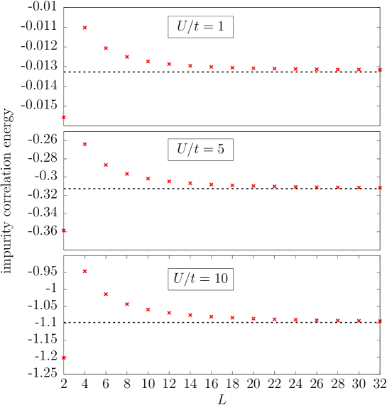
Figure 1: Accurate single-impurity ($M=1$) correlation density-functional energies computed at the DMRG level in the half-filled case. Results obtained for $L=64$ are shown in black dashed lines. See text for further details.

V Results and discussion

V.1 Half-filled case

In this work, SOET is applied to a relatively small 32-site ring. Nevertheless, as illustrated in the following, the number of sites is large enough so that there are no substantial finite-size errors in the calculation of density-functional energies. This can be easily seen in the half-filled case ($n=1$) where the exact embedding potential in Eq. (12) equals zero in the bath and $-U/2$ on the impurity sites (see Appendix A). The resulting impurity correlation density-functional energy [see Appendix C for further details] calculated at the DMRG level is shown in Fig. 1. The convergence towards the thermodynamic limit ($L\rightarrow+\infty$) is relatively fast. Note that the results obtained for $L=32$ and $L=64$ are almost undistinguishable.

Let us now focus on the calculation of double occupations which has been implemented according to Eq. (31) for various approximate functionals. Results are shown in Fig. 2.

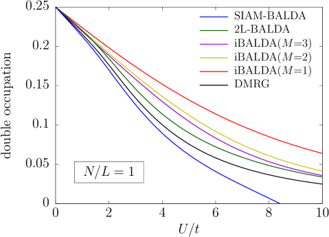
Figure 2: Double occupations obtained from half-filled SOET calculations for various single- and multiple-impurity DFAs. Both standard reference DMRG and iBALDA($M$=1) results are taken from Ref. Senjean et al. (2018). See text for further details.

While, in the weakly correlated regime and up to $U/t=5$, SIAM-BALDA gives the best results, it dramatically fails in stronger correlation regimes, as expected Senjean et al. (2018). In the particular strongly correlated half-filled case, SIAM-BALDA can be improved by interpolating between the weakly and strongly correlated regimes of the SIAM Senjean et al. (2018). Unfortunately, generalizing such an interpolation away from half-filling is not straightforward Senjean et al. (2018). On the other hand, 2L-BALDA performs relatively well for all the values of $U/t$. Turning to the multiple-impurity iBALDA approximation, the accuracy increases with the number of impurities, as expected, but the convergence towards DMRG is slow. Switching from two to three impurities slightly improves on the result, which is still less accurate than the (single-impurity) 2L-BALDA one. Interestingly, the same pattern is observed in DMET when the matching criterion involves the impurity site occupation only [see the noninteracting (NI) bath formulation in Ref. Bulik et al. (2014) and the Fig. 2 therein]. While our results would be improved by designing better $M$-dependent DFAs than iBALDA($M$), the performance of multiple-impurity DMET is increased when matching not only diagonal but also non-diagonal density matrix elements Knizia and Chan (2012); Bulik et al. (2014). Further connections between SOET and DMET are currently investigated and will be presented in a separate work.

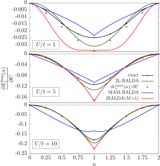
Figure 3: Single-impurity density-functional correlation energy derivative with respect to $U$ calculated for various $U/t$ values. The derivative shown for iBALDA($M$=1) is, by construction, the derivative of the per-site BALDA correlation energy. Exact results were obtained for the 8-site ring. See text and Appendix C for further details.

Returning to the single-impurity DFAs ($M=1$), it is quite instructive to plot the derivative in $U$ of the various functionals in order to analyze further the double occupations shown in Fig. 2. According to Eqs. (24) and (31), both full $e_{\rm c}(n)$ and impurity correlation energy derivatives should in principle be analyzed. However, at half-filling, and for any $U$ and $t$ values, BALDA becomes exact for $e_{\rm c}(n)$ when approaching the thermodynamic limit, by construction Lima et al. (2003). As a result, approximations in the impurity correlation functional will be the major source of errors which are purely functional-driven in the half-filled case, since the exact embedding potential is known (i.e. the correct uniform density profile is obtained when solving Eq. (12) in this case). Results are plotted with respect to the density in Fig. 3, thus providing a clear picture not only at half-filling but also around the latter density regime. The exact results obtained by Lieb maximization for the 8-site ring are used as reference [see the technical details in Appendix C]. Let us recall that, within iBALDA($M$=1), the impurity correlation energy is approximated with the full per-site correlation one $e_{\rm c}(n)$, which is then modeled at the BALDA level of approximation. The substantial (negative) difference between the exact full per-site and impurity correlation energy derivatives at half-filling (see Fig. 3), which is missing in iBALDA($M$=1), explains why the latter approximation systematically overestimates the double occupation. Interestingly, the derivative obtained with iBALDA($M$=1) at $n=1$, which is nothing but the derivative of the BALDA per-site correlation energy at half-filling, is essentially on top of its exact 8-site analog, thus confirming that finite-size effects are negligible. Turning to SIAM-BALDA, the derivative in $U$ of the impurity correlation energy turns out to be relatively accurate at $n=1$ for $U/t=1$ and $U/t=5$, thus leading to good double occupations in this regime of correlation. The derivative deteriorates for the larger $U/t=10$ value, as expected Senjean et al. (2018). Note finally that 2L-BALDA, where the impurity correlation functional is approximated by its analog for the Hubbard dimer, is the only approximation that provides reasonable derivatives in all correlation and density regimes. The stronger the correlation is, the more accurate the method is.

Let us finally discuss the per-site energies which have been computed according to Eq. (41) for the various DFAs. Results obtained at half-filling are shown in Fig. 4.

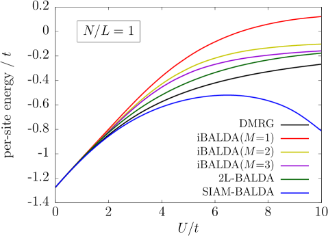
Figure 4: Per-site energies obtained from half-filled SOET calculations for various single- and multiple-impurity DFAs. Standard DMRG results are used as reference. See text for further details.

The discussion on the performance of each DFA for the double occupation turns out to hold also for the energy. This is simply due to the fact that the per-site non-interacting kinetic energy expression in Eq. (48) is highly accurate (it becomes exact in the thermodynamic limit), like the BALDA per-site correlation energy at half-filling (and therefore its derivative with respect to $t$). It then becomes clear, when comparing Eqs. (31) and (41), that, at half-filling, the only source of errors in the per-site energy is, like in the double occupation, the derivative in $U$ of the impurity correlation functional.

V.2 Functional-driven errors away from half-filling

Away from half-filling, the exact embedding potential is not uniform anymore in the bath Senjean et al. (2018), thus reflecting the dependence in the bath site occupations of the impurity correlation energy or, equivalently, of the per-site bath correlation energy [see Eqs. (12), (23), and (25)]. Such a dependence is neglected in all the DFAs used in this work, which induces errors in the density when the impurity-interacting wavefunction is computed self-consistently according to Eq. (12). This generates so-called density-driven errors in the calculation of both the energy and the double occupation Kim et al. (2013). The latter are analyzed in detail in Sec. V.3.

In this section, we focus on the functional-driven errors. In other words, all density-functional contributions are calculated with the exact uniform density, like in Sec. V.1. The corresponding per-site energies are shown in Fig. 5. Only the most challenging range of fillings (i.e. $0.6\leqslant N/L\leqslant 1$ Senjean et al. (2018)) is shown.

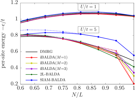
Figure 5: Per-site energies calculated in SOET for fillings in the range $0.6\leqslant N/L\leqslant 1$ with $U/t=1$ (upper curves) and $U/t=5$ (lower curves). Results obtained for various DFAs with exact (full lines) and self-consistently converged (dashed lines) densities are shown. The iBALDA($M$=1) and reference DMRG results are taken from Ref. Senjean et al. (2018). See text for further details.

It clearly appears that iBALDA($M$=1), while failing dramatically in the half-filled strongly correlated regime, performs relatively well away from half-filling in all correlation regimes. It is the best approximation in this regime of density. Increasing the number of impurities has only a substantial effect on the energy when approaching half-filling for large $U/t$ values. SIAM-BALDA performs reasonably well in the weakly correlated regime but not as well as the other functionals. In the same regime of correlation, 2L-BALDA stands in terms of accuracy between iBALDA and SIAM-BALDA in the lower density regime while giving the best result when approaching half-filling. The latter statement holds also in the strongly correlated regime.

In order to further analyze the performance of each functional, let us consider the derivative in $U$ of the single-impurity correlation functional shown in Fig. 3. Away from half-filling and in the strongly correlated regime, the full per-site and impurity correlation energies give the same derivative so that neglecting the last term in the right-hand side of Eq. (41), which is done in iBALDA($M$), is well justified. Interestingly, this feature is well reproduced by 2L-BALDA, where the impurity correlation energy obtained from the Hubbard dimer is combined with the per-site BALDA correlation energy [compare 2L-BALDA with iBALDA($M$=1) curves in the bottom panel of Fig. 3]. Obviously, SIAM-BALDA does not exhibit the latter feature which explains why it fails in this regime of correlation and density. Let us finally stress that, since BALDA provides an accurate description of the full per-site correlation energy in the strongly correlated regime, the second term in the right-hand side of Eq. (41) is expected to be well described in all the DFAs considered in this work (since they all use BALDA for this contribution). As shown in Fig. 6, this is actually the case [$\partial e^{\rm exact}_{\rm c}(n)/\partial t$ should be compared with the iBALDA($M$=1) derivative].

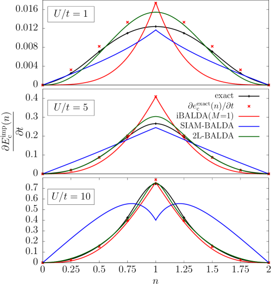
Figure 6: Single-impurity density-functional correlation energy derivative with respect to $t$ calculated for various $U/t$ values. The derivative shown for iBALDA($M$=1) is, by construction, the derivative of the per-site BALDA correlation energy. Exact results were obtained for the 8-site ring. See text and Appendix C for further details.

Turning to the weaker $U/t=1$ correlation regime, iBALDA($M$=1) underestimates the derivative in $t$ of the full per-site correlation energy [compare $\partial e^{\rm exact}_{\rm c}(n)/\partial t$ with iBALDA($M$=1) in Fig. 6] away from half-filling while setting to zero the derivative in $U$ of the per-site bath correlation functional whose accurate value is actually negative [compare $\partial e^{\rm exact}_{\rm c}(n)/\partial U$ with the exact impurity curve in Fig. 3]. The cancellation of errors leads to the relatively accurate results shown in Fig. 5. Turning to SIAM-BALDA in the same density and correlation regime, the (negative) derivative in $U$ of the per-site bath correlation energy is significantly overestimated [compare iBALDA($M$=1) with SIAM-BALDA in the top panel of Fig. 3], thus giving a total per-site energy lower than iBALDA($M$=1), as can be seen from the upper curves in Fig. 5. Interestingly, the latter derivative in $U$ is less overestimated when using 2L-BALDA. This explains why it performs better than SIAM-BALDA but still not as well as iBALDA($M$=1) which benefits from error cancellations.

V.3 Self-consistent results

We discuss in this section the results obtained by solving the density-functional impurity problem self-consistently [see Eq. (12)], thus accounting for not only functional-driven but also density-driven errors Kim et al. (2013). Self-consistently converged densities obtained on the impurity site(s) for various DFAs are shown in Figs. 7 and 8.

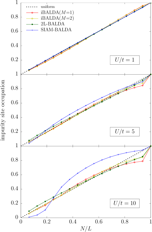
Figure 7: Self-consistently converged densities on the impurity site(s) plotted against the filling for various DFAs and $U/t$ values. For symmetry reasons, the two impurities in iBALDA($M$=2) have the same density.

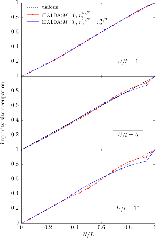
Figure 8: Self-consistently converged densities on the impurity sites plotted against the filling for iBALDA($M$=3) with different $U/t$ values. The central and neighboring impurity densities are denoted as $n_{1}^{\Psi^{\rm imp}_{M}}$ and $n_{0}^{\Psi^{\rm imp}_{M}}=n_{2}^{\Psi^{\rm imp}_{M}}$, respectively.

Note that, at half-filling ($n=1$), the exact embedding potential has been used, thus providing, for this particular density, the exact uniform density profile. Away from half-filling, approximate density-functional embedding potentials have been used, thus giving a density profile that is not strictly uniform anymore. Interestingly, for all the DFAs except SIAM-BALDA, the deviation from uniformity is more pronounced when approaching the half-filled strongly correlated regime. In the case of iBALDA, we notice that errors in the density are attenuated when increasing the number of impurities, as expected. On the other hand, SIAM-BALDA generates huge density errors for almost all fillings when the correlation is strong.

Turning to the weaker $U/t=1$ correlation regime, we note that, in contrast to iBALDA, both self-consistent SIAM-BALDA and 2L-BALDA calculations hardly break the exact uniform density profile (see the top panel of Fig. 7). This can be rationalized by plotting the various impurity correlation potentials (see Fig. 9).

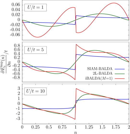
Figure 9: Single-impurity density-functional correlation potential obtained for various DFAs and $U/t$ values. The iBALDA($M$=1) potential is, by construction, the BALDA correlation potential.

Let us first stress that, for all the DFAs considered in this work, the correlation contribution to the embedding potential on site $i$ reads [see Eqs. (12), (21) (22), and (42)]

$$\dfrac{\partial e_{\rm c}(n_{i})}{\partial n_{i}}-\sum^{M-1}_{j=0}\delta_{ij}\dfrac{\partial E^{\rm imp}_{{\rm c},M}(n_{j})}{\partial n_{j}}.$$ (64)

The latter potential will therefore be equal to zero on the impurity sites if iBALDA is used. It will be uniform and equal to $\partial e_{\rm c}(n)/\partial n$ (at least in the first iteration of the self-consistent procedure as we start with a uniform density profile) in the bath. As shown in the top panel of Fig. 9 [see the iBALDA($M$=1) curve], in the weakly correlated regime, the latter potential, which is described with BALDA, is strongly attractive for densities lower than 0.6. This will induce a depletion of the density on the impurity sites, as clearly shown in the top panels of Figs. 7 and 8. The opposite situation is observed for densities in the range $0.6\leqslant n\leqslant 1$, as expected from the strongly repulsive character of the potential. Note that this charge transfer process, which is completely unphysical Akande and Sanvito (2010), is due to the incorrect linear behavior in $U$ of the BALDA correlation potential away from the strongly correlated regime Senjean et al. (2018). As readily seen from the first-order expansion in $U$ given in Eq. (32) of Ref. Senjean et al. (2018), the latter potential is expected to change sign at $n=(2/\pi)\arcsin\left(8/\pi^{2}\right)\approx 0.6$, which is in complete agreement with the top panel of Fig. 9. Returning to Eq. (64), for the single-impurity DFAs SIAM-BALDA and 2L-BALDA, the correlation contribution to the embedding potential reads $\partial e_{\rm c}(n)/\partial n-\partial E_{{\rm c}}^{\rm imp}(n_{0})/\partial n_{0}$ on the impurity site and still $\partial e_{\rm c}(n)/\partial n$ in the bath. As shown in the top panel of Fig. 9, SIAM-BALDA and 2L-BALDA impurity correlation potentials dot not deviate significantly from zero and, unlike iBALDA, they do not exhibit unphysical features in the weakly correlated regime, which explains why both DFAs give relatively good densities. Turning to iBALDA($M$=3) in the strongly correlated regime (middle and bottom panels of Fig. 8) and in the vicinity of half-filling, the impurity site 1 better reproduces the physical occupation $N/L$ than its nearest impurity neighbors (sites 0 and 2). It can be explained as follows. Site 1 is the central site of the ($M$=3)-impurity-interacting fragment, while sites 0 and 2 are directly connected to the (non-interacting and therefore unphysical) bath. As a consequence, site 1 “feels” the bath less than sites 0 and 2. It is, like in the physical system, surrounded by interacting sites. Interestingly, a similar observation has been made by Welborn et al. Welborn et al. (2016) within the Bootstrap-Embedding method, which is an improvement of DMET regarding the interaction between the fragment edge and the bath.

Let us now refocus on the poor performance of SIAM-BALDA in the strongly correlated regime. As shown in the middle and bottom panels of Fig. 9, the correlation part of the embedding potential on the impurity site [which corresponds to the difference between iBALDA($M$=1) and SIAM-BALDA curves] is, in this case, repulsive for densities lower than about 0.25 and strongly attractive in the range $0.25\leqslant n\leqslant 1$. The latter observation explains the large increase of density on the impurity site in the self-consistent procedure, as depicted in the bottom panel of Fig. 7.

Finally, as shown in Fig. 5, using self-consistently converged densities rather than exact (uniform) ones can induce substantial density-driven errors on the per-site energy, especially in the strongly correlated regime. Interestingly, both functional- and density-driven errors somehow compensate for 2L-BALDA around half-filling (see the lower curves in Fig. 5). This is not the case anymore exactly at half-filling since we used the exact embedding potential, thus removing density-driven errors completely. Regarding SIAM-BALDA, the large error in the converged density obtained for $N/L=0.6$ at $U/t=5$ (see the middle panel of Fig. 7) is reflected on the per-site energy. In this case, errors just accumulate. For larger fillings, SIAM-BALDA gives a better density on the impurity site but the functional-driven errors remain substantial.

V.4 Derivative discontinuity at half-filling

As illustrated in Ref. Senjean et al. (2018) in the special case of the atomic limit (i.e. $t=0$ or, equivalently, $U\rightarrow+\infty$), the impurity correlation potential on the impurity site should undergo a discontinuity at half-filling in the thermodynamic limit (even for finite values of $U$). This feature has fundamental and practical implications, in particular for the calculation of the fundamental gap. The latter quantity plays a crucial role in the description of the metal-insulator transition which, in the one-dimensional Hubbard model, appears as soon as the on-site repulsion is switched on ($U>0$) Lieb and Wu (1968).

As shown in Fig. 9, it is present in the iBALDA and SIAM-BALDA functionals, as a consequence of the hole-particle symmetry condition used in their construction. For the former functional, the feature is simply inherited from BALDA. On the other hand, even though the 2L-BALDA impurity correlation potential, which is extracted from the Hubbard dimer, also fulfills the particle-hole symmetry condition, it smoothly tends to 0 when approaching $n=1$. As a consequence, the potential exhibits no derivative discontinuity (DD) at half-filling when $U/t$ is finite. It only does when $U/t\rightarrow+\infty$ Senjean et al. (2017). As discussed by Dimitrov et al. Dimitrov et al. (2016), this is due to the fact that the dimer functional reproduces an intra-system steepening and not an inter-system DD. In other words, the change in density in the functional does not correspond to a change in the total number of electrons. The latter is indeed fixed to 2 in the dimer. Only the number of electrons on the impurity site varies. The problem becomes equivalent to describing an inter-system DD only when the impurity can be treated as an isolated system, which is indeed the case in the atomic (or, equivalently, strongly correlated) limit.

Note finally that, from a practical point of view, exhibiting a DD is not necessarily an advantage as convergence problems may occur around half-filling Lima et al. (2003). In this work, this problem has been bypassed by using the exact embedding potential at half-filling. Also, given that only 32 sites are considered, the closest uniform occupation to half-filling is obtained for 30 electrons, i.e. $n=0.9375$, which is far enough from the strictly half-filled situation. Convergence issues are expected to arise when approaching the thermodynamic limit since the density can then be much closer to 1. The practical solutions to this problem, which have been proposed for conventional KS calculations and use either a finite temperature Xianlong et al. (2012) or ad-hoc parameters Kurth et al. (2010); Karlsson et al. (2011); Ying et al. (2014), could in principle be implemented in SOET. This is left for future work. Note finally that, despite the absence of DD in the 2L-BALDA impurity correlation potential, the BALDA correlation potential is still employed for the bath within 2L-BALDA, which means that convergence issues will appear as soon as occupations in the bath are close to 1.

VI Conclusions and perspectives

Several extensions of a recent work Senjean et al. (2018) on site-occupation embedding theory (SOET) for model Hamiltonians have been explored. Exact expressions for per-site energies and double occupations have been derived for an arbitrary number of impurity sites. A simple $M$-impurity embedding density-functional approximation (DFA) based on the Bethe ansatz local density approximation (BALDA) and referred to as iBALDA($M$) has been proposed and tested on the one-dimensional Hubbard Hamiltonian. A new single-impurity DFA [referred to as 2L-BALDA] which combines BALDA with the impurity correlation functional of the two-level (2L) Hubbard system Senjean et al. (2017) has also been proposed. Finally, the performance of an existing DFA based on the single impurity Anderson model (SIAM) and BALDA Senjean et al. (2018), hence its name SIAM-BALDA, has been analyzed in further details in all correlation regimes. Both functional- and density-driven errors have been scrutinized. Among all the single-impurity DFAs, 2L-BALDA is clearly the one that performs the best in all density and correlation regimes. Unfortunately, the convergence of the (too) simple iBALDA approximation in the number of impurities towards the accurate DMRG results was shown to be slow. Better DFAs for multiple impurities are clearly needed. This is left for future work.

SOET can be extended further in many directions. First of all, substituting a Green function calculation for a many-body wavefunction one like DMRG is expected to reduce the computational cost of the method. From a formal point of view, this would also enable us to connect SOET with the dynamical mean-field theory (DMFT) [see, for example, Ref. Ayral et al. (2017)]. Note that the current formulation of SOET is canonical. It would be interesting to remap (density wise) the original fully-interacting Hubbard problem onto an open impurity system, in the spirit of the density matrix embedding theory (DMET). This may be achieved, in principle exactly, by combining SOET with partition DFT Elliott et al. (2010), or, in a more approximate way, by projecting the whole impurity-interacting problem in SOET onto a smaller embedded subspace. A Schmidt decomposition could be employed in the latter case Knizia and Chan (2012). Finally, an important step forward would be the exploration of SOET in higher dimensions. Work is currently in progress in all these directions.

Let us finally mention that the basic idea underlying SOET, which consists in extracting site (or orbital) occupations from a partially-interacting system, can be extended to an ab initio quantum chemical Hamiltonian by using, for example, its simplified seniority-zero expression Richardson (1963); Richardson and Sherman (1964); Limacher (2016). This will be presented in a separate work.

Appendix A Exact embedding potential at half-filling for multiple impurities

Let us consider any density $\mathbf{n}\equiv\{n_{i}\}_{i}$ summing up to a number $N=\sum_{i}n_{i}$ of electrons. Under hole-particle symmetry, this density becomes $(\underline{2}-\mathbf{n})\equiv\{2-n_{i}\}_{i}$ and the number of electrons equals $2L-N$ where $L$ is the number of sites. We will prove that these two densities give the same correlation energy for the $M$-impurity interacting system. Since, for any local potential $\mathbf{v}$, the variational principle in Eq. (5) reads as follows for an impurity-interacting system,

$$\mathcal{E}^{{\rm imp}}_{M}(\mathbf{v})=\underset{\mathbf{n}}{\rm min}\Big{\{}F^{\rm imp}_{M}(\mathbf{n})+(\mathbf{v}|\mathbf{n})\Big{\}},$$ (65)

which gives, for any density $\mathbf{n}$,

$$F^{\rm imp}_{M}(\mathbf{n})\geq\mathcal{E}^{{\rm imp}}_{M}(\mathbf{v})-(\mathbf{v}|\mathbf{n}),$$ (66)

thus leading to the Legendre–Fenchel transform expression,

$$F^{\rm imp}_{M}(\mathbf{n})=\underset{\mathbf{v}}{\rm sup}\Big{\{} \mathcal{E}^{{\rm imp}}_{M}(\mathbf{v})-(\mathbf{v}|\mathbf{n})\Big{\}}.$$ (67)

By applying a hole-particle symmetry transformation to Eq. (67) [we will now indicate the number of particles in the impurity-interacting energies for clarity], we obtain

$$F^{\rm imp}_{M}(\underline{2}-\mathbf{n})=\underset{\mathbf{v}}{\rm sup}\Big{\{}\mathcal{E}^{{\rm imp},2L-N}_{M}(\mathbf{v})-2\sum_{i}v_{i}+(\mathbf{v}|\mathbf{n})\Big{\}},$$

where $\mathcal{E}^{{\rm imp},2L-N}_{M}(\mathbf{v})$ is the ($2L-N$)-particle ground-state of the following $M$-impurity interacting Hamiltonian:

$$\hat{H}^{\rm imp}_{M}(\mathbf{v}) = -t\sum_{i\sigma}\left(\hat{c}_{i\sigma}^{\dagger}\hat{c}_{i+1\sigma}+\mathrm{H.c.}\right)+\sum_{i\sigma}v_{i}\hat{c}_{i\sigma}^{\dagger}\hat{c}_{i\sigma}$$ (69)

$$+U\sum_{i=0}^{M-1}\hat{c}_{i\uparrow}^{\dagger}\hat{c}_{i\uparrow}\hat{c}_{i\downarrow}^{\dagger}\hat{c}_{i\downarrow}.$$

Applying the hole-particle transformation to the creation and annihilation operators,

$$\hat{c}_{i\sigma}^{\dagger} \rightarrow \hat{b}_{i\sigma}^{\dagger}=(-1)^{i}\hat{c}_{i\sigma},$$

$$\hat{c}_{i\sigma} \rightarrow \hat{b}_{i\sigma}=(-1)^{i}\hat{c}_{i\sigma}^{\dagger},$$ (70)

to the $M$-impurity-interacting Hamiltonian in Eq. (69) leads to

$$\hat{H}^{\rm imp}_{M}(\mathbf{v}) = -t\sum_{i\sigma}\left(\hat{b}_{i\sigma}^{\dagger}\hat{b}_{i+1\sigma}+\mathrm{H.c.}\right)+\sum_{i\sigma}v_{i}\hat{b}_{i\sigma}\hat{b}_{i\sigma}^{\dagger}$$ (71)

$$+U\sum_{i=0}^{M-1}\hat{b}_{i\uparrow}\hat{b}_{i\uparrow}^{\dagger}\hat{b}_{i\downarrow}\hat{b}_{i\downarrow}^{\dagger},$$

or, equivalently,

$$\hat{H}^{\rm imp}_{M}(\mathbf{v}) = -t\sum_{i\sigma}\left(\hat{b}_{i\sigma}^{\dagger}\hat{b}_{i+1\sigma}+\mathrm{H.c.}\right)+2\sum_{i}v_{i}-\sum_{i\sigma}v_{i}\hat{b}_{i\sigma}^{\dagger}\hat{b}_{i\sigma}$$

$$+UM-U\sum_{i=0}^{M-1}\sum_{\sigma}\hat{b}_{i\sigma}^{\dagger}\hat{b}_{i\sigma}+U\sum_{i}\hat{b}_{i\uparrow}^{\dagger}\hat{b}_{i\uparrow}\hat{b}_{i\downarrow}^{\dagger}\hat{b}_{i\downarrow}.$$

Then, by substituting and shifting the potential as follows,

$$\tilde{v}_{i}=-v_{i}-U\sum_{j=0}^{M-1}\delta_{ij}$$ (73)

we finally obtain

$$\hat{H}^{\rm imp}_{M}(\mathbf{\tilde{v}}) = -t\sum_{i\sigma}\left(\hat{b}_{i\sigma}^{\dagger}\hat{b}_{i+1\sigma}+\mathrm{H.c.}\right)+2\sum_{i}v_{i}+\sum_{i\sigma}\tilde{v}_{i}\hat{b}_{i\sigma}^{\dagger}\hat{b}_{i\sigma}$$ (74)

$$+UM+U\sum_{i}\hat{b}_{i\uparrow}^{\dagger}\hat{b}_{i\uparrow}\hat{b}_{i\downarrow}^{\dagger}\hat{b}_{i\downarrow}.$$

As readily seen from Eqs. (69) and (74), the $(2L-N)$-electron ground-state energy $\mathcal{E}^{{\rm imp},2L-N}_{M}(\mathbf{v})$ of $\hat{H}^{\rm imp}_{M}(\mathbf{v})$ is connected to the $N$-electron ground-state energy $\mathcal{E}^{{\rm imp},N}_{M}(\mathbf{\tilde{v}})$ of $\hat{H}^{\rm imp}_{M}(\mathbf{\tilde{v}})$ by

$$\mathcal{E}^{{\rm imp},2L-N}_{M}(\mathbf{v})=\mathcal{E}^{{\rm imp},N}_{M}(\mathbf{\tilde{v}})+2\sum_{i}v_{i}+MU.$$ (75)

Introducing Eq. (75) into Eq. (A) leads to

$$F^{\rm imp}_{M}(\underline{2}-\mathbf{n}) = \underset{\mathbf{v}}{\rm sup}\left\{\mathcal{E}^{{\rm imp},N}_{M}(\tilde{\mathbf{v}})+(\mathbf{v}|\mathbf{n})\right\}+MU$$ (76)

$$= \underset{\tilde{\mathbf{v}}}{\rm sup}\left\{\mathcal{E}^{{\rm imp},N}_{M}(\tilde{\mathbf{v}})-(\tilde{\mathbf{v}}|\mathbf{n})\right\}+U\left(M-\sum_{i=0}^{M-1}n_{i}\right)$$

$$= F^{{\rm imp}}_{M}(\mathbf{n})+U\left(M-\sum_{i=0}^{M-1}n_{i}\right).$$

Note that the maximising potential in Eq. (76), denoted by $\tilde{v}^{\rm emb}_{M}(\mathbf{n})$, is nothing but the exact embedding potential $v^{\rm emb}_{M}(\mathbf{n})$ which restores the exact density profile $\mathbf{n}$, by definition:

$$\tilde{v}^{\rm emb}_{M,i}(\mathbf{n})=v^{\rm emb}_{M,i}(\mathbf{n}).$$ (77)

According to the shift in Eq. (73), this maximising potential is related to the maximising one in Eq. (A), denoted by $\mathbf{v}^{\rm emb}_{M}(\underline{2}-\mathbf{n})$, by

$$\tilde{v}_{M,i}^{\rm emb}(\mathbf{n})=-v^{\rm emb}_{M,i}(\underline{2}-\mathbf{n})-U\sum_{j=0}^{M-1}\delta_{ij}.$$ (78)

From the equality (77), it comes

$${v}_{M,i}^{\rm emb}(\underline{2}-\underline{n})=-{v}^{\rm emb}_{M,i}(\underline{n})-U\sum_{j=0}^{M-1}\delta_{ij}$$ (79)

thus leading to, at half-filling,

$${v}^{\rm emb}_{M,i}(\underline{1})=-\dfrac{U}{2}\sum_{j=0}^{M-1}\delta_{ij}.$$ (80)

Appendix B Fundamental relation between derivatives in $t$ and $U$ of the complementary bath per-site correlation energy for multiple impurities

If we denote $\mathbf{v}_{M}^{\rm emb}(\mathbf{n})$ the maximizing potential in the Legendre–Fenchel transform of Eq. (67), we deduce from the linearity in $t$ and $U$ of the impurity-interacting Hamiltonian that [the dependence in $t$ and $U$ is now introduced for clarity]

$$F^{\rm imp}_{M}(t,U,\mathbf{n})=\Bigg{[} t\dfrac{\partial\mathcal{E}^{{\rm imp}}_{M}(t,U,\mathbf{v})}{\partial t}$$ (81)

$$+U\dfrac{\partial\mathcal{E}^{{\rm imp}}_{M}(t,U,\mathbf{v})}{\partial U}\left.\Bigg{]}\right|_{\mathbf{v}=\mathbf{v}_{M}^{\rm emb}(\mathbf{n})},$$

thus leading to the fundamental relation

$$F^{\rm imp}_{M}(t,U,\mathbf{n}) = t\dfrac{\partial F^{\rm imp}_{M}(t,U,\mathbf{n})}{\partial t}$$ (82)

$$+U\dfrac{\partial F^{\rm imp}_{M}(t,U,\mathbf{n})}{\partial U},$$

as a consequence of the stationarity condition fulfilled by $\mathbf{v}_{M}^{\rm emb}(\mathbf{n})$. Since both the non-interacting kinetic energy [which is obtained when $U=0$] and the impurity Hx functional [first term in the right-hand side of Eq. (19)] fulfill the same relation, we conclude from the decomposition in Eq. (15) that

$$E^{\rm imp}_{{\rm c},M}(t,U,\mathbf{n}) = t\dfrac{\partial E^{\rm imp}_{{\rm c},M}(t,U,\mathbf{n})}{\partial t}$$ (83)

$$+U\dfrac{\partial E^{\rm imp}_{{\rm c},M}(t,U,\mathbf{n})}{\partial U}.$$

We finally obtain, by combining Eqs. (23), (83) and (C), the fundamental relation in Eq. (40).

Appendix C Lieb maximization and correlation energy derivatives for a single impurity

The impurity-interacting LL functional in Eq. (7) [we consider the particular case of a single impurity ($M=1$) in the following] can be rewritten as a Legendre–Fenchel transform  Fromager (2015); Senjean et al. (2017),

$$F^{\rm imp}(t,U,\mathbf{n})=\underset{\mathbf{v}}{\rm sup}\left\{\mathcal{E}^{\rm imp}(t,U,\mathbf{v})-(\mathbf{v}|\mathbf{n})\right\},$$ (84)

where $\mathcal{E}^{\rm imp}(t,U,\mathbf{v})$ is the ground-state energy of $\hat{T}+U\hat{n}_{0\uparrow}\hat{n}_{0\downarrow}+\sum_{i}v_{i}\hat{n}_{i}$. Note that the dependence in both $t$ and $U$ of $F^{\rm imp}(\mathbf{n})$ and $\mathcal{E}^{\rm imp}(\mathbf{v})$ has been introduced for clarity. The so-called Lieb maximization Lieb (1983) procedure described in Eq. (84) has been used in this work in order to compute accurate values of $F^{\rm imp}(t,U,\mathbf{n})$ and $T_{\rm s}(t,\mathbf{n})=F^{\rm imp}(t,U=0,\mathbf{n})$ for a 8-site ring. The impurity-interacting energy $\mathcal{E}^{\rm imp}(t,U,\mathbf{v})$ has been obtained by performing an exact diagonalization calculation based on the Lanczos algorithm Dagotto (1994). The impurity correlation energy is then obtained as follows,

$$E_{\rm c}^{\rm imp}(t,U,\mathbf{n})=F^{\rm imp}(t,U,\mathbf{n})-T_{\rm s}(t,\mathbf{n})-\dfrac{U}{4}n_{0}^{2}.$$ (85)

Since $\partial F^{\rm imp}(t,U,\mathbf{n})/\partial U=d^{\rm imp}(t,U,\mathbf{n})$ is the impurity site double occupation obtained for the maximizing potential in Eq. (84) [see Eq. (30) and Eq. (A5) in Ref. Senjean et al. (2018)], it comes from Eq. (85),

$$\dfrac{\partial E_{\rm c}^{\rm imp}(t,U,\mathbf{n})}{\partial U}=d^{\rm imp}(t,U,\mathbf{n})-\dfrac{n^{2}_{0}}{4}.$$ (86)

Moreover, since

$$t\dfrac{\partial F^{\rm imp}(t,U,\mathbf{n})}{\partial t}=T^{\rm imp}(t,U,\mathbf{n})$$

$$=F^{\rm imp}(t,U,\mathbf{n})-Ud^{\rm imp}(t,U,\mathbf{n})$$ (87)

is the impurity-interacting kinetic energy obtained for the maximizing potential in Eq. (84) [see Eq. (35) and Eq. (B6) in Ref. Senjean et al. (2018)], which gives in the non-interacting case $t\,\partial T_{\rm s}(t,\mathbf{n})/\partial t=T_{\rm s}(t,\mathbf{n})$, we recover from Eq. (85) the expression in Eq. (B8) of Ref. Senjean et al. (2018),

$$\dfrac{\partial E_{\rm c}^{\rm imp}(t,U,\mathbf{n})}{\partial t}=\dfrac{T^{\rm imp}(t,U,\mathbf{n})-T_{\rm s}(t,\mathbf{n})}{t},$$ (88)

which can be further simplified as follows,

$$\dfrac{\partial E_{\rm c}^{\rm imp}(t,U,\mathbf{n})}{\partial t} = \dfrac{E_{\rm c}^{\rm imp}(t,U,\mathbf{n})}{t}$$ (89)

$$+\dfrac{U}{t}\left[\dfrac{n_{0}^{2}}{4}-d^{\rm imp}(t,U,\mathbf{n})\right].$$

Interestingly, the derivatives in $t$ and $U$ are connected as follows, according to Eq. (86),

$$\dfrac{\partial E_{\rm c}^{\rm imp}(t,U,\mathbf{n})}{\partial t} = \dfrac{E_{\rm c}^{\rm imp}(t,U,\mathbf{n})}{t}$$ (90)

$$-\dfrac{U}{t}\dfrac{\partial E_{\rm c}^{\rm imp}(t,U,\mathbf{n})}{\partial U}.$$

Thus we recover Eq. (83) in the particular single-impurity case.

Similarly, in the fully-interacting case, the LL functional can be rewritten as follows, as a consequence of Eq. (5),

$$F(t,U,\mathbf{n})=\underset{\mathbf{v}}{\rm sup}\left\{{E}(t,U,\mathbf{v})-(\mathbf{v}|\mathbf{n})\right\},$$ (91)

where the $t$- and $U$-dependence in both $F(\mathbf{n})$ and $E(\mathbf{v})$ is now made explicit. From the correlation energy expression,

$$E_{\rm c}(t,U,\mathbf{n})=F(t,U,\mathbf{n})-T_{\rm s}(t,\mathbf{n})-\dfrac{U}{4}\sum_{i}n_{i}^{2},$$ (92)

and the expressions for the LL functional derivatives in $t$ and $U$ [those and their above-mentioned impurity-interacting analogs are deduced from the Hellmann-Feynman theorem],

$$\dfrac{\partial F(t,U,\mathbf{n})}{\partial U}=\sum_{i}d_{i}(t,U,\mathbf{n}),$$ (93)

and

$$t\dfrac{\partial F(t,U,\mathbf{n})}{\partial t} = T(t,U,\mathbf{n})$$ (94)

$$= F(t,U,\mathbf{n})-U\sum_{i}d_{i}(t,U,\mathbf{n}),$$

it comes

$$\dfrac{\partial E_{\rm c}(t,U,\mathbf{n})}{\partial U}=\sum_{i}d_{i}(t,U,\mathbf{n})-\dfrac{1}{4}\sum_{i}n_{i}^{2},$$ (95)

and

$$\dfrac{\partial E_{\rm c}(t,U,\mathbf{n})}{\partial t}=\dfrac{T(t,U,\mathbf{n})-T_{\rm s}(t,\mathbf{n})}{t}.$$ (96)

Note that $d_{i}(t,U,\mathbf{n})$ and $T(t,U,\mathbf{n})$, which have been introduced in Eqs. (93) and (94), denote the site $i$ double occupation and the total (fully-interacting) kinetic energy, respectively. Both are calculated for the maximizing potential in Eq. (91). For a uniform density profile $\underline{n}$, the per-site correlation energy reads

$$e_{\rm c}(t,U,n) = \dfrac{E_{\rm c}(t,U,\underline{n})}{L}$$ (97)

$$= \dfrac{1}{L}\Big{(}F(t,U,\underline{n})-T_{\rm s}(t,\underline{n})\Big{)}-\dfrac{U}{4}n^{2}.$$

Since, in this case, $d_{i}(t,U,\underline{n})=d(t,U,n)$ is site-independent, we finally obtain from Eqs. (94), (95) and (96),

$$\dfrac{\partial e_{\rm c}(t,U,{n})}{\partial U}=d(t,U,{n})-\dfrac{n^{2}}{4},$$ (98)

and

$$\dfrac{\partial e_{\rm c}(t,U,{n})}{\partial t} = \dfrac{F(t,U,\underline{n})-T_{\rm s}(t,\underline{n})}{tL}-\dfrac{U}{t}d(t,U,{n}).$$

By analogy with Eq. (89), the latter expression can be simplified as follows,

$$\dfrac{\partial e_{\rm c}(t,U,{n})}{\partial t} = \dfrac{e_{\rm c}(t,U,{n})}{t}+\dfrac{U}{t}\left[\dfrac{n^{2}}{4}-d(t,U,{n})\right],$$

or, equivalently (see Eq. (98)),

$$\dfrac{\partial e_{\rm c}(t,U,{n})}{\partial t} = \dfrac{e_{\rm c}(t,U,{n})}{t}-\dfrac{U}{t}\dfrac{\partial e_{\rm c}(t,U,{n})}{\partial U}.$$

Appendix D derivatives of BALDA

D.1 derivative with respect to $U$ and $t$

As readily seen in Eq. (31), the derivative of the complementary bath per-site correlation energy functional with respect to $U$ is necessary to compute double occupation in SOET. According to Eq. (24), it implies the derivative of the conventional per-site correlation energy, modelled with BALDA, which reads

$$\dfrac{\partial e_{\rm c}^{\rm BALDA}(n\leqslant 1,U/t)}{\partial U}=\dfrac{\partial\beta(U/t)}{\partial U}\left[\dfrac{-2t}{\pi}\sin\left(\dfrac{\pi n}{\beta(U/t)}\right)+\dfrac{2tn}{\beta(U/t)}\cos\left(\dfrac{\pi n}{\beta(U/t)}\right)\right]-\dfrac{n^{2}}{4},$$ (102)

and then for $n>1$:

$$\dfrac{\partial e_{\rm c}^{\rm BALDA}(n>1,U/t)}{\partial U}=\dfrac{\partial\beta(U/t)}{\partial U}\left[\dfrac{-2t}{\pi}\sin\left(\dfrac{\pi(2-n)}{\beta(U/t)}\right)+\dfrac{2t(2-n)}{\beta(U/t)}\cos\left(\dfrac{\pi(2-n)}{\beta(U/t)}\right)\right]+(n-1)-\dfrac{n^{2}}{4}$$

where $\partial\beta(U/t)/\partial U=(\partial\beta(U/t)/\partial(U/t))/t$, is computed with finite differences by solving Eq. (III.1) for $\beta(U/t)$.

The derivative with respect to $t$ are calculated according to Eq. (C).

D.2 derivative with respect to $n$

To get the correlation embedding potential, the derivatives of the correlation functionals with respect to $n$ is necessary. The derivative of the convention per-site density-functional correlation energy reads

$$\dfrac{\partial e_{\rm c}^{\rm BA}(n\leqslant 1)}{\partial n}=-2t\cos\left(\dfrac{\pi n}{\beta(U/t)}\right)+2t\cos\left(\dfrac{\pi n}{2}\right)-\dfrac{Un}{2},$$ (104)

and

$$\dfrac{\partial e_{\rm c}^{\rm BA}(n>1)}{\partial n}=2t\cos\left(\dfrac{\pi(2-n)}{\beta(U/t)}\right)-2t\cos\left(\dfrac{\pi(2-n)}{2}\right)+U-\dfrac{Un}{2}.$$ (105)

Appendix E derivatives of SIAM-BALDA

The derivatives of the SIAM-BALDA impurity correlation functional [Eq. (III.2.2)] are given with respect to $U$ for $n\leqslant 1$ as follows,

$$\dfrac{\partial E_{{\rm c},U/\Gamma\rightarrow 0}^{\rm SIAM}(U,\Gamma(t,n))}{\partial U}=-\dfrac{2\times 0.0369}{\pi}\left(\dfrac{U}{\Gamma(t,n)}\right)+\dfrac{4\times 0.0008}{\pi^{3}}\left(\dfrac{U}{\Gamma(t,n)}\right)^{3}.$$ (106)

The derivative with respect to $t$ is given according to Eq. (90). Then, the impurity correlation potential is determined by the derivative of the functional with respect to the occupation number $n$:

$$\dfrac{\partial E_{{\rm c},U/\Gamma\rightarrow 0}^{\rm SIAM}(U,\Gamma(t,n))}{\partial n}=\dfrac{\partial\Gamma(t,n)}{\partial n}\left.\dfrac{\partial E_{{\rm c},U/\Gamma\rightarrow 0}^{\rm SIAM}(U,\Gamma)}{\partial\Gamma}\right|_{\Gamma=\Gamma(t,n)},$$ (107)

where

$$\dfrac{\partial E_{{\rm c},U/\Gamma\rightarrow 0}^{\rm SIAM}(U,\Gamma)}{\partial\Gamma}=\dfrac{0.0369}{\pi}\left(\dfrac{U}{\Gamma}\right)^{2}-\dfrac{3\times 0.0008}{\pi^{3}}\left(\dfrac{U}{\Gamma}\right)^{4},$$ (108)

and

$$\dfrac{\partial\Gamma(t,n)}{\partial n}=t\left(\dfrac{-\dfrac{\pi}{2}\sin^{2}(\pi n/2)-(1+\cos(\pi n/2))\dfrac{\pi}{2}\cos(\pi n/2)}{\sin^{2}(\pi n/2)}\right)=-\dfrac{\pi t}{2}\left(\dfrac{1+\cos(\pi n/2)}{\sin^{2}(\pi n/2)}\right)=-\dfrac{\pi\Gamma(t,n)}{2\sin(\pi n/2)}.$$ (109)

If $n>1$, the particle-hole formalism imposes to use $\Gamma(t,2-n)$ instead of $\Gamma(t,n)$. The derivatives with respect to $n$ should be changed accordingly.

Appendix F derivatives of 2L-BALDA

F.1 Parametrization of the correlation energy of the dimer

In this section, we summarize the parametrization of the Hubbard dimer correlation energy by Carrascal and co-workers Carrascal et al. (2015, 2016), necessary to understand the following derivations. The equations coming from their paper are referred to as ($\&N)$, where $N$ is the number of the equation. We start from the definition of the correlation energy, where $n$ is the occupation of the site 0 and $u=U/2t$ is a dimensionless parameter,

$$E_{\rm c}^{\rm 2L}(U,n)=f(g,\rho)\Big{|}_{\begin{subarray}{l}g=g(\rho,u)\\ \rho=|n-1|\end{subarray}}-T_{\rm s}(n)-E_{\rm Hx}(U,n),$$ (110)

where 2L refers to “two-level”, and

$$T_{\rm s}(n)=-2t\sqrt{n(2-n)},~{}~{}~{}~{}E_{\rm Hx}(U,n)=U\left(1-n\left(1-\dfrac{n}{2}\right)\right).$$ (111)

To account for particle-hole symmetry of the functional, the variable $\rho=|n-1|$ is used rather than $n$ directly. We now simply follow the guidelines from Eq.($\&102$) to ($\&107$), leading to

$$f(g,\rho)=-2tg+Uh(g,\rho),$$ (112)

and

$$h(g,\rho)=\dfrac{g^{2}\left(1-\sqrt{1-\rho^{2}-g^{2}}\right)+2\rho^{2}}{2(g^{2}+\rho^{2})}.$$ (113)

Then, they proposed a first approximation to $g(\rho,u)$, denoted by the label 0:

$$g_{0}(\rho,u)=\sqrt{\dfrac{(1-\rho)(1+\rho(1+(1+\rho)^{3}ua_{1}(\rho,u)))}{1+(1+\rho)^{3}ua_{2}(\rho,u)}},$$ (114)

where

$$a_{i}(\rho,u)=a_{i1}(\rho)+ua_{i2}(\rho),~{}~{}~{}i=1,2$$ (115)

and

$$a_{21}(\rho)=\dfrac{1}{2}\sqrt{\dfrac{\rho(1-\rho)}{2}},~{}~{}~{}a_{12}(\rho)=\dfrac{1}{2}(1-\rho),~{}~{}~{}a_{11}(\rho)=a_{21}\left(1+\dfrac{1}{\rho}\right),~{}~{}~{}a_{22}(\rho)=\dfrac{a_{12}(\rho)}{2}.$$ (116)

Plugging $g=g_{0}(\rho,u)$ into $f(g,\rho)$ leads to the first parametrization of $E_{\rm c}^{2L}(n)$ in Eq. (110). In this work, we implemented the more accurate parametrization, given in Eq.($\&114$) Carrascal et al. (2016):

$$g_{1}(\rho,u)=g_{0}(\rho,u)+\left(u\left.\dfrac{\partial h(g,\rho)}{\partial g}\right|_{g=g_{0}(\rho,u)}-1\right)q(\rho,u),$$ (117)

and where $q(\rho,u)$ is given in Eq. ($\&115$) by Carrascal et al. (2016):

$$q(\rho,u)=\dfrac{(1-\rho)(1+\rho)^{3}u^{2}[(3\rho/2-1+\rho(1+\rho)^{3}ua_{2}(\rho,u))a_{12}(\rho)-\rho(1+(1+\rho)^{3}ua_{1}(\rho,u))a_{22}(\rho)]}{2g_{0}(\rho,u)(1+(1+\rho)^{3}ua_{2}(\rho,u))^{2}}.$$ (118)

The accurate pametrization of $E_{\rm c}^{2L}(n)$ is obtained by plugging this $g_{1}(\rho,u)$ into $f(g,\rho)$, instead of $g_{0}(\rho,u)$.
In order to obtain the impurity correlation energy, a simple scaling of the interaction parameter $U$ has to be applied on the conventional correlation energy, as demonstrated in Ref. Senjean et al. (2017) and given in Eq. (55), leading to

$$E_{\rm c}^{\rm imp,2L}(U,n)=E_{\rm c}^{2L}(U/2,n)=f(g,\rho)\Big{|}_{\begin{subarray}{l}g=g(\rho,u/2)\\ \rho=|n-1|\end{subarray}}-T_{\rm s}(n)-E_{\rm Hx}(U/2,n).$$ (119)

F.2 derivative with respect to $U$ and $t$

We compute the derivative with respect to the dimensionless parameter $u=U/2t$. The $\rho$- and $u$- dependence of $g(\rho,u)$ will be omitted for readability. Besides, many functions will be introduced, aiming to make the implementation and its numerical verification easier. Starting with

$$\dfrac{\partial E_{\rm c}^{\rm 2L}(n)}{\partial U} = \dfrac{1}{2t}\left.\dfrac{\partial f(g,\rho)}{\partial u}\right|_{\begin{subarray}{l}g=g(\rho,u)\\ \rho=|n-1|\end{subarray}}-\left(1+n\left(\dfrac{1}{2}n-1\right)\right),$$ (120)

the impurity correlation functional reads, according to Eq. (119),

$$\dfrac{\partial E_{\rm c}^{\rm imp,2L}(n)}{\partial U} = \dfrac{1}{4t}\left.\dfrac{\partial f(g,\rho)}{\partial u}\right|_{\begin{subarray}{l}g=g(\rho,u/2)\\ \rho=|n-1|\end{subarray}}-\dfrac{1}{2}\left(1+n\left(\dfrac{1}{2}n-1\right)\right),$$ (121)

with

$$\dfrac{\partial f(g,\rho)}{\partial u}=-2t\left(\dfrac{\partial g}{\partial u}-h(g,\rho)-u\times\dfrac{\partial h(g,\rho)}{\partial u}\right).$$ (122)

The derivative of $h(g,\rho)$ is quite easy, as its only $u$-dependence is contained in $g$, so that:

$$\dfrac{\partial h(g,\rho)}{\partial u}=\dfrac{\partial g}{\partial u}\dfrac{\partial h(g,\rho)}{\partial g},$$ (123)

with

$$\dfrac{\partial h(g,\rho)}{\partial g}=g\dfrac{g^{4}+3g^{2}\rho^{2}+2\rho^{2}\left(\rho^{2}-1-Y(g,\rho)\right)}{2\left(g^{2}+\rho^{2}\right)^{2}Y(g,\rho)},$$ (124)

where the function $Y(g,\rho)=\sqrt{1-g^{2}-\rho^{2}}$ has been introduced. For the first approximation, $g=g_{0}$ and

$$\dfrac{\partial g_{0}(\rho,u)}{\partial u}=\dfrac{\partial\sqrt{G(\rho,u)}}{\partial u}=\dfrac{\partial G(\rho,u)/\partial u}{2\sqrt{G(\rho,u)}},$$ (125)

where $G(\rho,u)=N(\rho,u)/D(\rho,u)$ and

$$N(\rho,u) = (1-\rho)\left[1+\rho\left(1+(1+\rho)^{3}ua_{1}(\rho,u)\right)\right],$$ (126)

$$D(\rho,u) = 1+(1+\rho)^{3}ua_{2}(\rho,u).$$ (127)

Their respective derivative with respect to $u$ reads

$$\dfrac{\partial N(\rho,u)}{\partial u} = (1-\rho)\rho(1+\rho)^{3}\left(a_{1}(\rho,u)+u\dfrac{\partial a_{1}(\rho,u)}{\partial u}\right),$$ (128)

$$\dfrac{\partial D(\rho,u)}{\partial u} = \left(1+\rho\right)^{3}\left(a_{2}(\rho,u)+u\dfrac{\partial a_{2}(\rho,u)}{\partial u}\right),$$ (129)

with

$$\dfrac{\partial a_{2}(\rho,u)}{\partial u}=a_{22}(\rho),~{}~{}~{}~{}\dfrac{\partial a_{1}(\rho,u)}{\partial u}=a_{12}(\rho).$$ (130)

Turning to the second approximation $g=g_{1}$ implemented in this work, one get from the derivative of Eq. (117),

$$\dfrac{\partial g_{1}}{\partial u} = \dfrac{\partial g_{0}}{\partial u}+\left(\left.\dfrac{\partial h(g,u)}{\partial g}\right|_{g=g_{0}}+u\dfrac{\partial}{\partial u}\left(\left.\dfrac{\partial h(g,u)}{\partial g}\right|_{g=g_{0}}\right)\right)q(\rho,u)+\left(u\left.\dfrac{\partial h(g,u)}{\partial g}\right|_{g=g_{0}}-1\right)\dfrac{\partial q(\rho,u)}{\partial u}.$$ (131)

For convenience, we introduce two functions $w(g,u)$ and $v(g,u)$ so that

$$\dfrac{\partial}{\partial u}\left(\dfrac{\partial h(g,u)}{\partial g}\right)=\left(\dfrac{\partial w(g,u)}{\partial u}v(g,u)-w(g,u)\dfrac{\partial v(g,u)}{\partial u}\right)\Big{/}v(g,u)^{2},$$ (132)

with

$$w(g,u) = g\left[g^{4}+3g^{2}\rho^{2}+2\rho^{2}\left(\rho^{2}-1-Y(g,\rho)\right)\right],$$ (133)

$$v(g,u) = 2Y(g,\rho)\left(g^{2}+\rho^{2}\right)^{2},$$ (134)

and

$$\dfrac{\partial w(g,u)}{\partial u} = \dfrac{\partial g}{\partial u}\left[g^{4}+3g^{2}\rho^{2}+2\rho^{2}\left(\rho^{2}-1-Y(g,\rho)\right)+g\left(4g^{3}+6g\rho^{2}+\dfrac{2\rho^{2}g}{Y(g,\rho)}\right)\right],$$ (135)

$$\dfrac{\partial v(g,u)}{\partial u} = g\left(g^{2}+\rho^{2}\right)\dfrac{\partial g}{\partial u}\left[\dfrac{-2\left(g^{2}+\rho^{2}\right)}{Y(g,\rho)}+8Y(g,\rho)\right].$$ (136)

Finally, the last term in Eq. (131) reads, for $q(\rho,u)=j(\rho,u)k(\rho,u)/l(\rho,u)$:

$$\dfrac{\partial q(\rho,u)}{\partial u}=\dfrac{\left(\dfrac{\partial j(\rho,u)}{\partial u}k(\rho,u)+j(\rho,u)\dfrac{\partial k(\rho,u)}{\partial u}\right)l(\rho,u)-j(\rho,u)k(\rho,u)\dfrac{\partial l(\rho,u)}{\partial u}}{l(\rho,u)^{2}}$$ (137)

with

$$j(\rho,u) = (1-\rho)(1+\rho)^{3}u^{2},$$ (138)

$$k(\rho,u) = \left(3\rho/2-1+\rho(1+\rho)^{3}ua_{2}(\rho,u)\right)a_{12}(\rho)-\rho\left(1+(1+\rho)^{3}\lambda ua_{1}(\rho,u)\right)a_{22}(\rho)$$ (139)

$$l(u) = 2g_{0}(u)\left[1+(1+\rho)^{3}\lambda ua_{2}(\rho,u,\lambda)\right]^{2},$$ (140)

and their derivative with respect the $u$:

$$\dfrac{\partial j(\rho,u)}{\partial u} = 2(1-\rho)(1+\rho)^{3}\lambda u$$ (141)

$$\dfrac{\partial k(u)}{\partial u} = a_{12}(\rho)\left[\rho(1+\rho)^{3}\left(a_{2}(\rho,u)+u\dfrac{\partial a_{2}(\rho,u)}{\partial u}\right)\right]-a_{22}(\rho)\left[\rho(1+\rho)^{3}\left(a_{1}(\rho,u)+u\dfrac{\partial a_{1}(\rho,u)}{\partial u}\right)\right]$$ (142)

$$\dfrac{\partial l(u)}{\partial u} = 4g_{0}(u)\left[1+(1+\rho)^{3}ua_{2}(\rho,u)\right](1+\rho)^{3}\left(a_{2}(\rho,u)+u\dfrac{\partial a_{2}(\rho,u)}{\partial u}\right)+2\dfrac{\partial g_{0}}{\partial u}\left[1+(1+\rho)^{3}\lambda ua_{2}(\rho,u)\right]^{2}.$$ (143)

The derivative with respect to $t$ is given according to Eq. (90).

F.3 derivative with respect to $n$

Regarding the derivative with respect to $n$ which is necessary to get the embedded correlation potential, it comes

$$\dfrac{\partial E_{\rm c}^{\rm imp,2L}(n)}{\partial n}=\dfrac{\partial\rho}{\partial n}\left.\dfrac{f(g,\rho)}{\partial\rho}\right|_{\begin{subarray}{l}g=g(\rho,u/2)\\ \rho=|n-1|\end{subarray}}-\dfrac{\partial\mathcal{T}_{s}(n)}{\partial n}+\dfrac{U}{2}(1-n)$$ (144)

where $\partial\rho/\partial n={\text{sign($n-1$)}}$ and

$$\dfrac{\partial\mathcal{T}_{s}(n)}{\partial n}=-\dfrac{2t(1-n)}{\sqrt{n(2-n)}}.$$ (145)

We start with

$$\dfrac{\partial f(g,\rho)}{\partial\rho}=-2t\dfrac{\partial g}{\partial\rho}+U\dfrac{\partial h(g,\rho)}{\partial\rho},$$ (146)

where, for the first parametrization using $g=g_{0}(\rho,u)$,

$$\dfrac{\partial g_{0}}{\partial\rho} = =\dfrac{1}{2g_{0}D(\rho,u)}\left(\dfrac{\partial N(\rho,u)}{\partial\rho}-g_{0}^{2}\dfrac{\partial D(\rho,u)}{\partial\rho}\right),$$ (147)

with

$$\dfrac{\partial N(\rho,u)}{\partial\rho} = -1+(1-2\rho)\left(1+(1+\rho)^{3}ua_{1}(\rho,u)\right)+\rho u(1-\rho)(1+\rho)^{2}\left(3a_{1}(\rho,u)+(1+\rho)\dfrac{\partial a_{1}(\rho,u)}{\partial\rho}\right),$$ (148)

$$\dfrac{\partial D(\rho,u)}{\partial\rho} = u(1+\rho)^{2}\left(3a_{2}(\rho,u)+(1+\rho)\dfrac{\partial a_{2}(\rho,u)}{\partial\rho}\right),$$ (149)

and

$$\dfrac{\partial a_{1}(\rho,u)}{\partial\rho} = \dfrac{\partial a_{11}(\rho)}{\partial\rho}+u\dfrac{\partial a_{12}(\rho)}{\partial\rho},~{}~{}~{}~{}~{}\dfrac{\partial a_{2}(\rho,u)}{\partial\rho}=\dfrac{\partial a_{21}(\rho)}{\partial\rho}+u\dfrac{\partial a_{22}(\rho)}{\partial\rho}$$ (150)

$$\dfrac{\partial a_{12}(\rho)}{\partial\rho} = 2\dfrac{\partial a_{22}(\rho)}{\partial\rho}=-\dfrac{1}{2},~{}~{}~{}~{}\dfrac{\partial a_{21}(\rho)}{\partial\rho}=\dfrac{1-2\rho}{8\sqrt{(1-\rho)\rho/2}},~{}~{}~{}~{}\dfrac{\partial a_{11}(\rho)}{\partial\rho}=\dfrac{\partial a_{21}(\rho)}{\partial\rho}\left(1+\dfrac{1}{\rho}\right)-\dfrac{1}{\rho^{2}}a_{21}(\rho).$$ (151)

Then, the right term in the right hand side of Eq. (146) is derived as:

$$\dfrac{\partial h(g,\rho)}{\partial\rho} = \dfrac{1}{2(g^{2}+\rho^{2})}\left(4\rho+2g\dfrac{\partial g}{\partial\rho}\left(1-Y(g,\rho)\right)+g^{2}\dfrac{g(\partial g/\partial\rho)+\rho}{Y(g,\rho)}\right)-\dfrac{g(\partial g/\partial\rho)+\rho}{(g^{2}+\rho^{2})^{2}}\left(2\rho^{2}+g^{2}\left(1-Y(g,\rho)\right)\right).$$

Turning to the second parametrization $g=g_{1}$, the derivative with respect to $\rho$ leads to

$$\dfrac{\partial g_{1}}{\partial\rho}=\dfrac{\partial g_{0}}{\partial\rho}+\left(u\left.\dfrac{\partial h(g,\rho)}{\partial g}\right|_{g=g_{0}}-1\right)\dfrac{\partial q(\rho,u)}{\partial\rho}+u\dfrac{\partial}{\partial\rho}\left(\left.\dfrac{\partial h(g,\rho)}{\partial g}\right|_{g=g_{0}}\right)q(\rho,u)$$ (153)

with

$$\dfrac{\partial}{\partial\rho}\left(\dfrac{\partial h(g,\rho)}{\partial g}\right) = \dfrac{-(\partial g/\partial\rho)(g^{2}+\rho^{2})+4g(g(\partial g/\partial\rho)+\rho)}{(g^{2}+\rho^{2})^{3}}\left(2\rho^{2}+g^{2}(1-Y(g,\rho))\right)$$ (154)

$$-\dfrac{g}{(g^{2}+\rho^{2})^{2}}\left(4\rho+2g\dfrac{\partial g}{\partial\rho}\left(1-Y(g,\rho)\right)+g^{2}\dfrac{g(\partial g/\partial\rho)+\rho}{Y(g,\rho)}\right)-\dfrac{g(\partial g/\partial\rho)+\rho}{(g^{2}+\rho^{2})^{2}}\left(2g(1-Y(g,\rho))+\dfrac{g^{3}}{Y(g,\rho)}\right)$$

$$+\dfrac{1}{2(g^{2}+\rho^{2})}\left(2\dfrac{\partial g}{\partial\rho}(1-Y(g,\rho))+\dfrac{2g\rho}{Y(g,\rho)}+\dfrac{5g^{2}(\partial g/\partial\rho)}{Y(g,\rho)}+g^{3}\dfrac{g(\partial g/\partial\rho)+\rho}{Y(g,\rho)^{3}}\right).$$

Finally,

$$\dfrac{\partial q(\rho,u)}{\partial\rho}=\left(\dfrac{\partial P(\rho,u)}{\partial\rho}Q(\rho,u)-P(\rho,u)\dfrac{\partial Q(\rho,u)}{\partial\rho}\right)\Big{/}Q(\rho,u)^{2},$$ (155)

with

$$\dfrac{\partial P(\rho,u)}{\partial\rho} = \left(3(1-\rho)(1+\rho)^{2}-(1+\rho)^{3}\right)u^{2}\left[\left(\dfrac{3\rho}{2}-1+\rho(1+\rho)^{3}ua_{2}(\rho,u)\right)a_{12}(\rho)-\rho\left(1+(1+\rho)^{3}ua_{1}(\rho,u)\right)a_{22}(\rho)\right]$$ (156)

$$+(1-\rho)(1+\rho)^{3}u^{2}\left[\left(\dfrac{3}{2}+3u(1+\rho)^{2}\rho a_{2}(\rho,u)+u(1+\rho)^{3}\left(a_{2}(\rho,u)+\rho\dfrac{\partial a_{2}(\rho,u)}{\partial\rho}\right)\right)a_{12}(\rho)\right.$$

$$+\left.\left(\dfrac{3\rho}{2}-1+\rho(1+\rho)^{3}ua_{2}(\rho,u)\right)\dfrac{\partial a_{12}(\rho)}{\partial\rho}-\left(\rho\dfrac{\partial a_{22}(\rho)}{\partial\rho}+a_{22}(\rho)\right)\left(1+(1+\rho)^{3}ua_{1}(\rho,u)\right)\right.$$

$$\left.-\rho a_{22}(\rho)\left(3(1+\rho)^{2}ua_{1}(\rho,u)+(1+\rho)^{3}u\dfrac{\partial a_{1}(\rho,u)}{\partial\rho}\right)\right]$$

$$\dfrac{\partial Q(\rho,u)}{\partial\rho} = 2\dfrac{\partial g_{0}}{\partial\rho}\left(1+(1+\rho)^{3}ua_{2}(\rho,u)\right)^{2}+4g_{0}\left(1+(1+\rho)^{3}ua_{2}(\rho,u)\right)u\left(3(1+\rho)^{2}a_{2}(\rho,u)+(1+\rho)^{3}\dfrac{\partial a_{2}(\rho,u)}{\partial\rho}\right).$$

References

- Pulay (1983) P. Pulay, Chem. Phys. Lett. 100, 151 (1983).
- Saebo and Pulay (1993) S. Saebo and P. Pulay, Annu. Rev. Phys. Chem. 44, 213 (1993).
- Hampel and Werner (1996) C. Hampel and H.-J. Werner, J. Chem. Phys. 104, 6286 (1996).
- Sun and Chan (2016) Q. Sun and G. K.-L. Chan, Acc. Chem. Res. 49, 2705 (2016).
- Georges and Kotliar (1992) A. Georges and G. Kotliar, Phys. Rev. B 45, 6479 (1992).
- Georges et al. (1996) A. Georges, G. Kotliar, W. Krauth, and M. J. Rozenberg, Rev. Mod. Phys. 68 (1996).
- Kotliar and Vollhardt (2004) G. Kotliar and D. Vollhardt, Phys. Today 57, 53 (2004).
- Held (2007) K. Held, Adv. Phys. 56, 829 (2007).
- Zgid and Chan (2011) D. Zgid and G. K.-L. Chan, J. Chem. Phys. 134 (2011).
- Hettler et al. (1998) M. Hettler, A. Tahvildar-Zadeh, M. Jarrell, T. Pruschke, and H. Krishnamurthy, Phys. Rev. B 58, R7475 (1998).
- Hettler et al. (2000) M. Hettler, M. Mukherjee, M. Jarrell, and H. Krishnamurthy, Phys. Rev. B 61, 12739 (2000).
- Lichtenstein and Katsnelson (2000) A. Lichtenstein and M. Katsnelson, Phys. Rev. B 62, R9283 (2000).
- Kotliar et al. (2001) G. Kotliar, S. Y. Savrasov, G. Pálsson, and G. Biroli, Phys. Rev. Lett. 87, 186401 (2001).
- Maier et al. (2005) T. Maier, M. Jarrell, T. Pruschke, and M. H. Hettler, Rev. Mod. Phys. 77, 1027 (2005).
- Rohringer et al. (2018) G. Rohringer, H. Hafermann, A. Toschi, A. Katanin, A. Antipov, M. Katsnelson, A. Lichtenstein, A. Rubtsov, and K. Held, Rev. Mod. Phys. 90, 025003 (2018).
- Kotliar et al. (2006) G. Kotliar, S. Y. Savrasov, K. Haule, V. S. Oudovenko, O. Parcollet, and C. A. Marianetti, Rev. Mod. Phys. 78, 865 (2006).
- Sun and Kotliar (2002) P. Sun and G. Kotliar, Phys. Rev. B 66, 085120 (2002).
- Biermann et al. (2003) S. Biermann, F. Aryasetiawan, and A. Georges, Phys. Rev. Lett. 90, 086402 (2003).
- Karlsson (2005) K. Karlsson, J. Phys. Condens. Matter 17, 7573 (2005).
- Boehnke et al. (2016) L. Boehnke, F. Nilsson, F. Aryasetiawan, and P. Werner, Phys. Rev. B 94, 201106 (2016).
- Werner and Casula (2016) P. Werner and M. Casula, J. Phys. Condens. Matter 28, 383001 (2016).
- Nilsson et al. (2017) F. Nilsson, L. Boehnke, P. Werner, and F. Aryasetiawan, Phys. Rev. Materials 1, 043803 (2017).
- Kananenka et al. (2015) A. A. Kananenka, E. Gull, and D. Zgid, Phys. Rev. B 91, 121111 (2015).
- Lan et al. (2015) T. N. Lan, A. A. Kananenka, and D. Zgid, J. Chem. Phys. 143, 241102 (2015).
- Zgid and Gull (2017) D. Zgid and E. Gull, New J. Phys. 19, 023047 (2017).
- Lan et al. (2017) T. N. Lan, A. Shee, J. Li, E. Gull, and D. Zgid, Phys. Rev. B 96, 155106 (2017).
- Knizia and Chan (2012) G. Knizia and G. K.-L. Chan, Phys. Rev. Lett. 109, 186404 (2012).
- Knizia and Chan (2013) G. Knizia and G. K.-L. Chan, J. Chem. Theory Comput. 9, 1428 (2013).
- Bulik et al. (2014) I. W. Bulik, G. E. Scuseria, and J. Dukelsky, Phys. Rev. B 89, 035140 (2014).
- Zheng and Chan (2016) B.-X. Zheng and G. K.-L. Chan, Phys. Rev. B 93, 035126 (2016).
- Wouters et al. (2016) S. Wouters, C. A. Jiménez-Hoyos, Q. Sun, and G. K.-L. Chan, J. Chem. Theory Comput. (2016).
- Wouters et al. (2017) S. Wouters, C. A. Jiménez-Hoyos, and G. K.-L. Chan, “Five years of density matrix embedding theory,” in Fragmentation (Wiley-Blackwell, 2017) Chap. 8, p. 227.
- Rubin (2016) N. C. Rubin, arXiv preprint arXiv:1610.06910 (2016).
- Tsuchimochi et al. (2015) T. Tsuchimochi, M. Welborn, and T. Van Voorhis, J. Chem. Phys. 143, 024107 (2015).
- Welborn et al. (2016) M. Welborn, T. Tsuchimochi, and T. Van Voorhis, J. Chem. Phys. 145, 074102 (2016).
- Ayral et al. (2017) T. Ayral, T.-H. Lee, and G. Kotliar, Phys. Rev. B 96, 235139 (2017).
- Frésard and Wölfle (1992) R. Frésard and P. Wölfle, Int. J. Mod. Phys. B 6, 685 (1992).
- Lechermann et al. (2007) F. Lechermann, A. Georges, G. Kotliar, and O. Parcollet, Phys. Rev. B 76, 155102 (2007).
- Fromager (2015) E. Fromager, Mol. Phys. 113, 419 (2015).
- Senjean et al. (2017) B. Senjean, M. Tsuchiizu, V. Robert, and E. Fromager, Mol. Phys. 115, 48 (2017).
- Senjean et al. (2018) B. Senjean, N. Nakatani, M. Tsuchiizu, and E. Fromager, Phys. Rev. B 97, 235105 (2018).
- Chayes et al. (1985) J. Chayes, L. Chayes, and M. B. Ruskai, J. Stat. Phys. 38, 497 (1985).
- Gunnarsson and Schönhammer (1986) O. Gunnarsson and K. Schönhammer, Phys. Rev. Lett. 56, 1968 (1986).
- Capelle and Campo Jr. (2013) K. Capelle and V. L. Campo Jr., Phys. Rep. 528, 91 (2013).
- Hohenberg and Kohn (1964) P. Hohenberg and W. Kohn, Phys. Rev. 136, B864 (1964).
- Levy (1979) M. Levy, Proceedings of the National Academy of Sciences 76, 6062 (1979).
- Lima et al. (2002) N. Lima, L. Oliveira, and K. Capelle, Europhys. Lett. 60, 601 (2002).
- Lima et al. (2003) N. A. Lima, M. F. Silva, L. N. Oliveira, and K. Capelle, Phys. Rev. Lett. 90, 146402 (2003).
- Capelle et al. (2003) K. Capelle, N. Lima, M. Silva, and L. Oliveira, in The Fundamentals of Electron Density, Density Matrix and Density Functional Theory in Atoms, Molecules and the Solid State (Springer, 2003) p. 145.
- Yamada (1975) K. Yamada, Prog. Theo. Phys. 53, 970 (1975).
- Carrascal et al. (2015) D. J. Carrascal, J. Ferrer, J. C. Smith, and K. Burke, J. Phys. Condens. Matter 27, 393001 (2015).
- Carrascal et al. (2016) D. J. Carrascal, J. Ferrer, J. C. Smith, and K. Burke, J. Phys. Condens. Matter. 29, 019501 (2016).
- White (1992) S. R. White, Phys. Rev. Lett. 69, 2863 (1992).
- White (1993) S. R. White, Phys. Rev. B 48, 10345 (1993).
- Verstraete et al. (2008) F. Verstraete, V. Murg, and J. I. Cirac, Adv. Phys. 57, 143 (2008).
- Schollwöck (2011) U. Schollwöck, Ann. Phys. 326, 96 (2011).
- (57) N. Nakatani, [Online]. https://github.com/naokin/mpsxx.
- Kim et al. (2013) M.-C. Kim, E. Sim, and K. Burke, Phys. Rev. Lett. 111, 073003 (2013).
- Akande and Sanvito (2010) A. Akande and S. Sanvito, Phys. Rev. B 82, 245114 (2010).
- Lieb and Wu (1968) E. H. Lieb and F. Y. Wu, Phys. Rev. Lett. 20, 1445 (1968).
- Dimitrov et al. (2016) T. Dimitrov, H. Appel, J. I. Fuks, and A. Rubio, New J. Phys. 18, 083004 (2016).
- Xianlong et al. (2012) G. Xianlong, A.-H. Chen, I. Tokatly, and S. Kurth, Phys. Rev. B 86, 235139 (2012).
- Kurth et al. (2010) S. Kurth, G. Stefanucci, E. Khosravi, C. Verdozzi, and E. Gross, Phys. Rev. Lett. 104, 236801 (2010).
- Karlsson et al. (2011) D. Karlsson, A. Privitera, and C. Verdozzi, Phys. Rev. Lett. 106, 116401 (2011).
- Ying et al. (2014) Z.-J. Ying, V. Brosco, and J. Lorenzana, Phys. Rev. B 89, 205130 (2014).
- Elliott et al. (2010) P. Elliott, K. Burke, M. H. Cohen, and A. Wasserman, Phys. Rev. A 82, 024501 (2010).
- Richardson (1963) R. Richardson, Phys. Lett. 3, 277 (1963).
- Richardson and Sherman (1964) R. Richardson and N. Sherman, Nucl. Phys. 52, 221 (1964).
- Limacher (2016) P. A. Limacher, J. Chem. Phys. 145, 194102 (2016).
- Lieb (1983) E. H. Lieb, Int. J. Quantum Chem. 24, 243 (1983).
- Dagotto (1994) E. Dagotto, Rev. Mod. Phys. 66, 763 (1994).