Abstract

The QCD axion solves the strong $CP$ problem and represents an attractive particle candidate for cold dark matter (CDM). However, quantum fluctuations of the axion field during inflation easily result in large CDM isocurvature perturbations that are in conflict with observations of the cosmic microwave background (CMB). In this paper, we demonstrate how this problem can be solved in low-scale models of hybrid inflation that may emerge from supersymmetric grand unified theories. We consider both F-term hybrid inflation (FHI) and D-term hybrid inflation (DHI) in supergravity, explicitly taking into account the effect of hidden-sector supersymmetry breaking. We discuss the production of cosmic strings and show how the soft terms in the scalar potential readily allow to achieve the correct scalar spectral index. In both cases, we are able to identify large regions in parameter space that are consistent with all constraints. In particular, we find that evading the CDM isocurvature constraint always requires a small Yukawa or gauge coupling of $\mathcal{O}\left(10^{-3}\right)$ or smaller. This translates into upper bounds on the gravitino mass of $\mathcal{O}\left(10^{5}\right)\,\textrm{GeV}$ in FHI and $\mathcal{O}\left(10^{9}\right)\,\textrm{GeV}$ in DHI. Our results point to interesting scenarios in well-motivated parameter regions that will be tested in future axion and CMB experiments.

1 Introduction

The Peccei-Quinn (PQ) mechanism [1, 2] is a viable and attractive solution to the strong $CP$ problem in quantum chromodynamics (QCD). It is based on the idea to promote the effective QCD vacuum angle $\bar{\theta}$ to a pseudoscalar field — known as the axion $a=f_{a}\,\bar{\theta}$ [3, 4] — which dynamically relaxes the QCD vacuum energy until it reaches a ground state that preserves charge parity ($CP$) invariance [5]. The axion field is almost invisible, i.e., it is a weakly coupled gauge singlet whose couplings are suppressed by a large decay constant $f_{a}$. In concrete realizations of the PQ mechanism [6, 7, 8, 9], the axion is identified as the pseudo-Nambu-Goldstone boson of a global $U(1)_{\rm PQ}$ symmetry that exhibits a nonvanishing $SU(3)$ color anomaly (quantified in terms of an anomaly coefficient $N$) and that is spontaneously broken at a high energy scale $v_{\rm PQ}=Nf_{a}$. As has become clear over the years, the QCD axion entails an extremely rich phenomenology in particle physics, astrophysics, and cosmology (for reviews, see [10, 11, 12, 13, 14]), which makes it a primary target in the hunt for new physics beyond the Standard Model (BSM). The axion can, in particular, be copiously produced in the early Universe, which renders it a well-motivated particle candidate for dark matter (DM) [15, 16, 17]. Together, these observations distinguish the PQ mechanism as a testable and predictive BSM scenario that not only solves the strong $CP$ problem but that automatically also accounts for the DM relic density.

In the context of inflationary cosmology [18, 19, 20, 21], one has to discriminate between two different implementations of the PQ mechanism, depending on the magnitude of the axion decay constant $f_{a}$. First, consider the case in which the Hubble rate during inflation, $H_{\rm inf}$, always exceeds $f_{a}$. In this scenario, spontaneous PQ symmetry breaking (PQSB) only occurs after inflation in the radiation-dominated era. Similarly, if the maximal temperature in the early Universe, $T_{\rm max}$, is greater than $f_{a}$, the PQ symmetry is thermally restored after inflation, and it only becomes spontaneously broken at lower temperatures as soon as $T\sim f_{a}$. In either case, PQ symmetry breaking occurs at late times, which results in the production of cosmic strings. During the QCD phase transitions, these axion strings turn into the boundaries of domain walls [22]. One can show that, for an anomaly coefficient $N$, there are actually $N$ different types of domain wall solutions, which is why $N$ is also referred to as the domain wall number. For $N>1$, the domain walls are stable, so that they begin to dominate the total energy density of the Universe soon after their formation. This is known as the domain wall problem of the postinflationary PQSB scenario. There are several ways out of this problem. An obvious solution is to simply restrict oneself to a trivial domain wall number, $N=1$. This is, e.g., possible if only one vectorlike exotic quark contributes to the PQ color anomaly (see [23, 24] for a recent example). In this case, the domain walls are unstable and the entire string-wall network decays, which results in a certain fraction of the total axion DM relic density [25, 26, 27, 28]. Alternatively, one may explicitly break the PQ symmetry by means of higher-dimensional operators in the effective theory [29], so that the domain walls become unstable even for a nontrivial domain wall number, $N>1$. However, this solution requires some tuning, as the tight upper bound on the effective QCD theta angle, $\left|\bar{\theta}\right|\lesssim 10^{-10}$ [30], restricts the allowed amount of explicit PQ symmetry breaking.

The arguably simplest solution to the domain wall problem is to presume that the PQ symmetry is already broken during inflation and never becomes restored afterwards. This preinflationary PQSB scenario corresponds to the second possibility of implementing the PQ mechanism in the context of inflationary cosmology. It is realized for large values of the axion decay constant,

$$f_{a}\gtrsim\max\left\{H_{\rm inf},T_{\rm max}\right\}\,.$$ (1)

In this scenario, all dangerous topological defects that form at early times are vastly diluted by the exponential expansion during inflation. We emphasize that this solution neither constrains the value of the domain wall number $N$ nor requires particular assumptions about higher-dimensional operators in the effective theory. Instead, one now has to deal with the implications of a spontaneously broken global symmetry during inflation and, in particular, with the presence of the massless axion field. Just like the inflaton field, the axion field develops quantum fluctuations during inflation. These axion fluctuations are nearly scale-invariant and uncorrelated with the adiabatic curvature perturbations, such that they turn into cold dark matter (CDM) isocurvature perturbations after inflation [31, 32, 33, 34, 35, 36, 37]. Axion isocurvature perturbations have attracted a great deal of attention in the last two decades [38, 39, 40, 41, 42, 43, 44, 45, 46, 47, 48, 49, 50, 51, 52, 53, 54, 55, 56, 57, 58, 59, 60, 61, 62, 63, 64, 65]. On the one hand, the prediction of measurable axion isocurvature perturbations is exciting, as it implies that one may not only be able to probe the QCD axion in laboratory experiments on Earth but also via observations of the anisotropies in the cosmic microwave background (CMB). On the other hand, it represents an important restriction of the preinflationary PQSB scenario, since the amplitude of the isocurvature power spectrum is tightly constrained by the measurements of the PLANCK satellite [66, 67]. This issue is sometimes referred to as the axion isocurvature perturbations problem. The PLANCK constraint on the primordial isocurvature fraction especially implies an upper bound on the inflationary Hubble rate $H_{\rm inf}$ that is in conflict with typical values of $H_{\rm inf}$ in high-scale models of inflation. The preinflationary PQSB scenario therefore calls for low-scale inflation with a small Hubble rate.

In this paper, we will demonstrate that the CDM isocurvature constraint on the inflationary Hubble scale can be easily satisfied in low-scale models of hybrid inflation [37, 68]. To this end, we will revisit both F-term hybrid inflation (FHI) [69, 70] and D-term hybrid inflation (DHI) [71, 72] in supergravity (SUGRA). These models represent promising inflationary scenarios. They can be naturally embedded into supersymmetric grand unified theories (GUTs) and, hence, establish a connection between inflation and grand unification. A particularly attractive feature is that both scenarios end in a so-called waterfall transition, i.e., a rapid second-order phase transition that can be identified with the spontaneous breaking of a local GUT symmetry. The key idea behind our analysis is to explicitly account for the spontaneous breaking of supersymmetry (SUSY) in a hidden sector. As we will see, hidden-sector SUSY breaking results in a number of soft terms in the scalar potential that can be used to achieve consistency with the CMB data. In FHI, the dominant soft term turns out to be a linear tadpole term, while in DHI, the leading soft term is a quadratic mass term. In both cases, the size of the soft terms is controlled by the gravitino mass $m_{3/2}$. Therefore, by tuning the soft terms against the radiative corrections in the scalar potential, one is always able to realize a particularly flat inflaton potential, i.e., a very small slow-roll parameter $\varepsilon\ll 1$. At the same time, the energy scale in the tree-level potential, $V_{0}^{1/4}$, can always be chosen so as to reproduce the amplitude of the scalar power spectrum, $A_{s}\propto V_{0}/\varepsilon$. Together, these two relations yield a powerful mechanism to suppress the inflationary Hubble scale $H_{\rm inf}\propto V_{0}^{1/2}$. In addition, the dependence of the slow-roll parameter $\varepsilon$ on $m_{3/2}$ links the gravitino mass to the Hubble rate, $\varepsilon\left(m_{3/2},\cdots\right)\propto H_{\rm inf}^{2}$. For a given $H_{\rm inf}$, we, thus, have to choose a gravitino mass of a certain magnitude. Otherwise, the scalar potential will be either too steep or too flat to obtain the correct value for $A_{s}$. For this reason, the CDM isocurvature constraint on $H_{\rm inf}$ can also be used to derive upper bounds on $m_{3/2}$.

To find the viable regions in parameter space, we will study the slow-roll dynamics of FHI and DHI in a fully analytical fashion. That is, wherever possible, we will refrain from resorting to the usual numerical methods that are typically employed in the literature. On the one hand, this will allow us to determine the implications of the CDM isocurvature constraint on the model parameters of hybrid inflation in an analytical and transparent manner. On the other hand, our analysis will be rather general, so that our results are actually well suited to be used in further investigations of hybrid inflation, beyond the question of axion isocurvature perturbations. The main result of our analysis will be that, in both FHI and DHI, the inflationary Hubble scale can be pushed down to a sufficiently small value — provided that an appropriate coupling constant is set to a value of $\mathcal{O}\left(10^{-3}\right)$ or smaller. In FHI, this coupling corresponds to the inflaton Yukawa coupling $\kappa$ in the superpotential, while in DHI, it typically corresponds to the gauge coupling $g$ in the waterfall sector. In both cases, such a small coupling constant is stable against radiative corrections and, hence, technically natural. In supersymmetric hybrid inflation, the isocurvature perturbations problem of the QCD axion can therefore be solved without any unnatural fine-tuning of model parameters.

The remainder of this paper is organized as follows. In the next section, we will review the CDM isocurvature constraint on $H_{\rm inf}$ in the preinflationary PQSB scenario. In Secs. 3 and 4, we will then discuss in turn the inflationary dynamics of FHI and DHI. In doing so, we will explicitly distinguish between scenarios with a comparatively large field excursion during inflation and scenarios with a very small field excursion during inflation. In Sec. 5, we will summarize our main results and discuss a number of interesting benchmark points in parameter space. For readers that are primarily interested in our constraints on parameter space and less interested in the technical details of our slow-roll analysis, we note that most of the results derived in this paper are included in one way or another in Fig. 5. Finally, Sec. 6 contains our conclusions and a brief outlook.

2 Axion isocurvature perturbations

We begin by reviewing the CDM isocurvature constraint on $H_{\rm inf}$ in the preinflationary PQSB scenario. First, we note that most properties of the QCD axion are fixed by its decay constant $f_{a}$. This includes the axion mass $m_{a}$, which can be obtained via an explicit calculation in chiral perturbation theory [83] as well as via numerical lattice simulations [84]. The results of both approaches agree within their respective uncertainties and yield the following expression for $m_{a}$,

$$m_{a}\simeq 57.0\,\textrm{\lx@text@micro\hskip 0.5pteV}\left(\frac{10^{11}\,\textrm{GeV}}{f_{a}}\right)\,.$$ (2)

Next, let us consider the axion energy density $\Omega_{a}h^{2}$. If the PQ symmetry is already broken before the end of inflation, the only contribution to the axion abundance in the present epoch follows from the standard vacuum misalignment mechanism [15, 16, 17]. In this case, $\Omega_{a}h^{2}$ ends up being a function of the axion decay constant $f_{a}$ and the initial value of the QCD vacuum angle, $\bar{\theta}_{\rm ini}=a_{\rm ini}/f_{a}$, in the observable patch of the Universe. For a small initial theta angle, $\left|\bar{\theta}_{\rm ini}\right|\ll\pi$, and assuming that the axion field begins to coherently oscillate before the QCD phase transition, one finds [23, 24]

$$\Omega_{a}h^{2}\simeq 0.65\left(\frac{\bar{\theta}_{\rm ini}}{10^{-2}}\right)^{2}\left(\frac{f_{a}}{10^{16}\,\textrm{GeV}}\right)^{1.17}\,.$$ (3)

This expression can be further refined by accounting for anharmonic effects in the vicinity of the local maximum in the axion scalar potential, i.e., for $\left|\bar{\theta}_{\rm ini}\right|\sim\pi$. Therefore, following the analyses in [85, 48], we shall modify Eq. (3) by incorporating a correction factor $C_{\rm anh}$ of the following form,

$$\Omega_{a}h^{2}\simeq 0.65\left(\frac{\bar{\theta}_{\rm ini}}{10^{-2}}\right)^{2}\left(\frac{C_{\rm anh}\,f_{a}}{10^{16}\,\textrm{GeV}}\right)^{1.17}\,,\quad C_{\rm anh}=1-\ln\left(1-\frac{\bar{\theta}_{\rm ini}^{2}}{\pi^{2}}\right)\,.$$ (4)

This prediction needs to be compared with the PLANCK result for the DM relic density [66],

$$\Omega_{\rm DM}h^{2}\simeq 0.12\,.$$ (5)

Suppose that axions make up a fraction $F_{\rm DM}^{a}\in\left[0,1\right]$ of the total DM abundance. The PLANCK constraint in Eq. (5) can then be used to solve Eq. (4) for the initial theta angle as a function of $f_{a}$,

$$\bar{\theta}_{\rm ini}=\left(F_{\rm DM}^{a}\right)^{1/2}\,\bar{\theta}_{\rm ini}^{\rm DM}\,,\quad F_{\rm DM}^{a}=\frac{\Omega_{a}}{\Omega_{\rm DM}}\,,\quad\bar{\theta}_{\rm ini}^{\rm DM}\simeq 4.3\times 10^{-3}\left(\frac{10^{16}\,\textrm{GeV}}{f_{a}}\right)^{0.59}\,,$$ (6)

which is valid and self-consistent in the small-$\bar{\theta}$ regime where $C_{\rm anh}\approx 1$. Also, note that $\bar{\theta}_{\rm ini}^{\rm DM}$ represents the initial theta angle that is necessary to achieve pure axion DM. The main lesson from Eq. (6) is that large values of the axion decay constant, $f_{a}\gg 10^{12}\,\textrm{GeV}$, only lead to viable axion DM if the initial theta angle is somewhat tuned. However, it is important to realize that this kind of tuning is very different from a brute-force tuning of the QCD vacuum angle in a theory without a dynamical axion field. First of all, note that, even for an axion decay constant as large as $f_{a}\sim M_{\rm Pl}$, the required tuning is only at the level of $1$ out of roughly $10^{4}$. This is certainly less drastic than tuning $\bar{\theta}$ to a value less than $10^{-10}$ by hand. But the main conceptual difference is that, in the QCD axion scenario, the initial theta angle becomes susceptible to anthropic reasoning. In a theory including a dynamical axion field, $\bar{\theta}_{\rm ini}$ controls the final DM abundance (see Eq. (4)). As pointed out by Linde long ago [88], it may, thus, well be that an apparently tuned theta angle in our observable Universe is, in fact, the consequence of environmental selection during inflation (see also [89, 90]).

If the axion field is already present during inflation, it will develop quantum fluctuations that exhibit the typical standard deviation $\sigma_{a}$ of a massless scalar field in an expanding de Sitter space,

$$\sigma_{a}=\left<\delta a^{2}\right>^{1/2}\simeq\frac{H_{\rm inf}}{2\pi}\,,$$ (7)

which translates into the following standard deviation for the dynamical theta angle $\bar{\theta}=a/f_{a}$,

$$\sigma_{\bar{\theta}}=\frac{1}{f_{a}}\left<\delta a^{2}\right>^{1/2}\simeq\frac{H_{\rm inf}}{2\pi f_{a}}\,.$$ (8)

By virtue of Eq. (4), these fluctuations in the initial theta angle are responsible for the emergence of CDM density isocurvature (CDI) perturbations around the time of the QCD phase transition (i.e., at the onset of the coherent axion oscillations) [31, 32, 33, 34, 35, 36, 37]. Because the axion fluctuations during inflation are independent of the quantum fluctuations of the inflaton field, the resulting CDI perturbations are uncorrelated with the adiabatic curvature perturbations. Up to corrections of $\mathcal{O}\left(\sigma_{\bar{\theta}}^{3}\right)$, the magnitude of the axion isocurvature perturbations at a given length scale, $S_{\rm iso}$, simply follows from the derivative of the (logarithm of the) axion energy density w.r.t. the initial theta angle (see, e.g., [48]),

$$S_{\rm iso}=\frac{\delta\Omega_{\rm DM}}{\Omega_{\rm DM}}=F_{\rm DM}^{a}\,\frac{\delta\Omega_{a}}{\Omega_{a}}\simeq F_{\rm DM}^{a}\,\frac{\partial\ln\Omega_{a}}{\partial\,\bar{\theta}_{\rm ini}}\,\sigma_{\bar{\theta}}=F_{\rm DM}^{a}\,\frac{2\sigma_{\bar{\theta}}}{\bar{\theta}_{\rm ini}}\,.$$ (9)

The square of this expression yields the amplitude of the isocurvature power spectrum $\mathcal{P}_{\rm iso}$,

$$\mathcal{P}_{\rm iso}=\left|S_{\rm iso}\right|^{2}\simeq\left(F_{\rm DM}^{a}\,\frac{2\sigma_{\bar{\theta}}}{\bar{\theta}_{\rm ini}}\right)^{2}\simeq\left(F_{\rm DM}^{a}\,\frac{H_{\rm inf}}{\pi f_{a}\bar{\theta}_{\rm ini}}\right)^{2}=F_{\rm DM}^{a}\mathcal{P}_{\rm iso}^{\rm DM}\,,$$ (10)

which holds in the small-$\bar{\theta}$ regime and up to corrections of $\mathcal{O}\left(\sigma_{\bar{\theta}}^{4}\right)$. In Eq. (10), we again factored out the dependence on the axion DM fraction $F_{\rm DM}^{a}$. In the case of pure axion DM, one has

$$\mathcal{P}_{\rm iso}^{\rm DM}\simeq\left(\frac{H_{\rm inf}}{\pi f_{a}\bar{\theta}_{\rm ini}^{\rm DM}}\right)^{2}\,.$$ (11)

The PLANCK data can be used to place an upper bound on the primordial isocurvature fraction

$$\beta_{\rm iso}\left(k\right)=\frac{\mathcal{P}_{\rm iso}\left(k\right)}{\mathcal{P}_{\rm adi}\left(k\right)+\mathcal{P}_{\rm iso}\left(k\right)}\,.$$ (12)

Here, we emphasize that both power spectra $\mathcal{P}_{\rm adi}$ and $\mathcal{P}_{\rm iso}$ are in general scale-dependent and, hence, functions of the wavenumber $k$. The amplitude of the adiabatic curvature perturbations, $\mathcal{P}_{\rm adi}$, is fixed by the observed amplitude of the primordial scalar power spectrum, $\mathcal{P}_{\rm adi}\simeq 2.2\times 10^{-9}$ at the CMB pivot scale $k=0.05\,\textrm{Mpc}^{-1}$ [67]. For an uncorrelated mixture of adiabatic and CDI modes and assuming a unit isocurvature spectral index, $n_{\rm iso}=1$, the PLANCK 2015 data results in [67],

$$\beta_{\rm iso}\left(k\right)<0.038\,,\quad k=0.05\,\textrm{Mpc}^{-1}\quad\textrm{(95\,\% CL; TT,\,TE,\,EE\,$+$\,lowP)}\,,$$ (13)

which translates into an upper bound on the amplitude of the isocurvature power spectrum of

$$\mathcal{P}_{\rm iso}\lesssim 8.7\times 10^{-11}\,.$$ (14)

Making use of Eq. (10), we, thus, obtain the following upper bound on the inflationary Hubble rate,

$$H_{\rm inf}\lesssim 1.3\times 10^{9}\,\textrm{GeV}\left(\frac{1}{F_{\rm DM}^{a}}\right)^{1/2}\left(\frac{f_{a}}{10^{16}\,\textrm{GeV}}\right)^{0.42}\,.$$ (15)

Two comments are in order in view of this bound. First, we stress that Eq. (15) is, indeed, a very tight restriction on the allowed set of inflationary models. To see this more explicitly, recall that, in standard single-field slow-roll inflation, $H_{\rm inf}$ uniquely determines the tensor-to-scalar ratio $r$,

$$r=\frac{A_{t}}{A_{s}}=\frac{2}{A_{s}}\left(\frac{H_{\rm inf}}{\pi\,M_{\rm Pl}}\right)^{2}\simeq 1.5\times 10^{-11}\left(\frac{H_{\rm inf}}{10^{9}\,\textrm{GeV}}\right)^{2}\,,$$ (16)

where $A_{s}$ and $A_{t}$ denote the amplitudes of the primordial scalar and tensor power spectra, respectively. The small values of $H_{\rm inf}$ that are required by Eq. (15) therefore imply that $r$ must be unobservably small. This can also be formulated by rewriting Eq. (15) as an upper bound on $r$,

$$r\lesssim 2.4\times 10^{-11}\left(\frac{1}{F_{\rm DM}^{a}}\right)\left(\frac{f_{a}}{10^{16}\,\textrm{GeV}}\right)^{0.83}\,,$$ (17)

which needs to be contrasted with the current upper bound on the tensor-to-scalar ratio, $r\lesssim 0.1$ [67]. Any detection of nonzero $r$ in the near future would therefore immediately rule out all low-scale models of inflation that are in accord with Eq. (15). A second comment regarding Eq. (15) is that the dependence on the axion DM fraction $F_{\rm DM}^{a}$ is actually rather mild. Even if axions only account for, say, 10 % of the total DM abundance, the bound is only relaxed by roughly a factor $3$. For this reason, it is impossible to evade the constraint on $H_{\rm inf}$ in high-scale models of inflation (where $H_{\rm inf}\sim 10^{13}\cdots 10^{14}\,\textrm{GeV}$) without completely abandoning the idea of an axion DM fraction.

Thus far, we only focused on the small-$\bar{\theta}$ regime, where the anharmonic correction factor in $C_{\rm anh}$ in Eq. (4) can be neglected. However, for completeness, we mention that all of the steps above can also be repeated including $C_{\rm anh}$. For $\left|\bar{\theta}_{\rm ini}\right|\sim\pi$, this can be even done analytically. For small values of the axion decay constant $f_{a}$ and large values of $\left|\bar{\theta}_{\rm ini}\right|$, a straightforward calculation yields

$$H_{\rm inf}\lesssim 88\,\textrm{GeV}\left(\frac{1}{F_{\rm DM}^{a}}\right)^{0.15}e^{-12.64\,\left(E-1\right)}\,,\quad E=\left(\frac{F_{\rm DM}^{a}}{1}\right)^{0.85}\left(\frac{10^{10}\,\textrm{GeV}}{f_{a}}\right)\,.$$ (18)

This is an extremely strong constraint that can only be satisfied in more or less unconventional scenarios of inflation. In the following, we will therefore focus our attention on the bound in Eq. (15) and its implications for hybrid inflation. The bound in Eq. (18) will only appear in Fig. 5 where it serves the purpose to mark the boundary of the viable parameter space at small values of $f_{a}$.

3 Low-scale F-term hybrid inflation

3.1 Model setup and scalar potential

We now turn to supersymmetric hybrid inflation and determine the implications of the CDM isocurvature constraint in Eq. (15) on its parameter space. First, we will consider FHI supplemented with a hidden SUSY-breaking sector [92]. The relevant terms in the superpotential are given as

$$W=\kappa\,S\,\Phi\bar{\Phi}-\mu_{S}^{2}S+\mu_{X}^{2}X+w\,,$$ (19)

where $S$ denotes the chiral inflaton field, $\Phi$ and $\bar{\Phi}$ are two chiral waterfall fields, and $X$ is the Polonyi field. $\kappa$ is a dimensionless Yukawa coupling, while $\mu_{S}$ and $\mu_{X}$ denote the inflaton and Polonyi F-term mass scales, respectively. $w$ represents a constant contribution to the superpotential that arises in consequence of $R$ symmetry breaking. Its value needs to be tuned so as to achieve a vanishingly small cosmological constant (CC) in the true vacuum after inflation. The first two terms on the right-hand side (RHS) of Eq. (19) represent the superpotential of FHI, while the last two terms coincide with the superpotential of the standard Polonyi model of spontaneous SUSY breaking [93]. For simplicity, we shall assume that all chiral fields possess a canonical Kähler potential to leading order,

$$K=S^{\dagger}S+\Phi^{\dagger}\Phi+\bar{\Phi}^{\dagger}\bar{\Phi}+X^{\dagger}X+\frac{\chi}{M_{\rm Pl}^{2}}\,S^{\dagger}S\,X^{\dagger}X+\cdots\,.$$ (20)

Here, we include a higher-dimensional coupling between $S$ and $X$ whose strength is controlled by a dimensionless coefficient $\chi$. This operator is allowed by all symmetries and expected to be present in the effective theory at energies below the Planck scale, $M_{\rm Pl}\simeq 2.44\times 10^{18}\,\textrm{GeV}$. As we will see, it contributes to the soft SUSY-breaking parameters in the scalar inflaton potential. The ellipsis in Eq. (20) stands for further higher-dimensional operators that are negligible for the present discussion. We only remark that the Kähler potential should also contain a higher-dimensional self-interaction for the Polonyi field, $K\supset-\left|X\right|^{4}/M_{*}^{2}$ for some high mass scale $M_{*}$, such that $X$ is always safely stabilized at the origin in field space. This can, e.g., be achieved via additional couplings to matter fields in the hidden sector (see [94, 95, 96] for an example based on strong gauge dynamics). Provided that $\left<X\right>=0$ for all times during and after inflation, the parameters $\mu_{X}$, $w$, and $m_{3/2}$ can be related to each other based on the requirement that the CC must vanish in the true vacuum after inflation,

$$w=m_{3/2}\,M_{\rm Pl}^{2}\,,\quad m_{3/2}=\frac{\mu_{X}^{2}}{\sqrt{3}\,M_{\rm Pl}}\,.$$ (21)

The waterfall fields $\Phi$ and $\bar{\Phi}$ transform in conjugate representations of a gauge group $G$ that may be part of a larger GUT gauge group, $G\subseteq G_{\rm GUT}$. The inflaton and the Polonyi field are supposed to transform as complete singlets under the group $G$. In the following, we will restrict ourselves to the simplest scenario of an Abelian gauge group, $G=U(1)$. In this case, the gauge interactions in the waterfall sector result in a D-term scalar potential of the form

$$V_{D}=\frac{g^{2}}{2}\left[q\left(\left|\phi\right|^{2}-\left|\bar{\phi}\right|^{2}\right)\right]^{2}\,,$$ (22)

where $g$ denotes the $G$ gauge coupling constant and $+q$ and $-q$ are the $G$ gauge charges of the waterfall fields $\Phi$ and $\bar{\Phi}$. In the following, we will set $q=1$ without loss of generality. The situation with arbitrary charge $q$ can always be restored by redefining the gauge coupling, $g\rightarrow g^{\prime}=g/q$. The D-term scalar potential ensures that the vacuum expectation values (VEVs) of the two waterfall fields coincide at all times, $\big{<}\Phi\big{>}=\big{<}\bar{\Phi}\big{>}$. Apart from this, it is irrelevant for the dynamics of FHI. During inflation, the two waterfall fields are stabilized at the origin in field space, $\big{<}\Phi\big{>}=\big{<}\bar{\Phi}\big{>}=0$, while after inflation (i.e., after the waterfall phase transition), both fields acquire a nonzero VEV,

$$\big{<}\Phi\big{>}=\big{<}\bar{\Phi}\big{>}=\frac{v}{\sqrt{2}}\,,\quad v=\sqrt{2}\,\frac{\mu_{S}}{\kappa^{1/2}}\,.$$ (23)

The VEV $v$ characterizes the energy scale at which $G$ becomes spontaneously broken. It is normalized such that it corresponds to the aligned VEVs of the two real Higgs scalars contained in $\Phi$ and $\bar{\Phi}$.

The relevant contribution to the tree-level potential stems from the F-term scalar potential,

$$V_{F}=e^{z}\left[\left(1-z+z^{2}\right)\mu_{S}^{4}+\sqrt{2}\left(2-z\right)\mu_{S}^{2}\,m_{3/2}\,s\,\cos\varphi+\frac{1-\chi\left(3-z\right)}{2\left(1+\chi\,z\right)}\,m_{3/2}^{2}\,s^{2}\right]\,.$$ (24)

This potential is understood to be evaluated along the inflationary trajectory where $\big{<}\Phi\big{>}=\big{<}\bar{\Phi}\big{>}=0$. The real field variables $s$, $\varphi$, and $z$ are related to the original complex inflaton field $S$ as follows,

$$S=\frac{s}{\sqrt{2}}\,e^{i\varphi}\,,\quad S^{*}=\frac{s}{\sqrt{2}}\,e^{-i\varphi}\,,\quad z=\frac{\left|S\right|^{2}}{M_{\rm Pl}^{2}}=\frac{s^{2}}{2\,M_{\rm Pl}^{2}}\,.$$ (25)

Remarkably enough, all terms in $V_{F}$ — except for the constant contribution to the vacuum energy density — correspond to corrections that only arise in the context of SUGRA. An investigation of FHI without the proper inclusion of SUGRA effects is therefore highly incomplete [97, 98]. At field values below the Planck scale, the F-term scalar potential in Eq. (24) can be expanded as follows,

$$V_{F}=V_{F}^{0}+c_{s}\left(1+\frac{z}{2}\right)s+\frac{1}{2}\,m_{s}^{2}\,s^{2}+\frac{1}{24}\,\lambda_{s}\,s^{4}+\mathcal{O}\left(s^{6}\right)\,.$$ (26)

Here, the leading term $V_{F}^{0}=\mu_{S}^{4}$ corresponds to the F-term scalar potential in the global-SUSY limit. It is constant and sets the inflationary Hubble scale during FHI. To good approximation, we have

$$H_{\rm inf}\simeq\frac{\left(V_{F}^{0}\right)^{1/2}}{\sqrt{3}\,M_{\rm Pl}}=\frac{\mu_{S}^{2}}{\sqrt{3}\,M_{\rm Pl}}\,.$$ (27)

Eq. (26) also contains a linear tadpole term whose strength is controlled by the coefficient $c_{s}$,

$$c_{s}=2\sqrt{2}\,\mu_{S}^{2}\,m_{3/2}\cos\varphi\,.$$ (28)

This term has important consequences for the dynamics of FHI [92, 99, 100, 101, 102]. In particular, it introduces a dependence on the complex inflaton phase $\varphi$ (through the $\cos\varphi$ factor in $c_{s}$), which breaks the rotational invariance in the complex inflaton plane. FHI consequently turns into a two-field model of inflation whose full dynamics can only be captured by a comprehensive analysis of all possible trajectories in the complex plane [102]. However, for the purposes of this paper, we will restrict ourselves to the case of inflation along the negative real axis where $\varphi=\pi$. This is the simplest case and motivated by the fact that it will provide us with the strongest bounds on parameter space. As will become clear later on, our final results are therefore valid and applicable for all trajectories in the complex plane and do not rely on any assumption regarding the particular choice of trajectory. Besides that, we note that also the other coefficients in Eq. (24) have an important physical meaning. $m_{s}^{2}$ and $\lambda_{s}$ denote the inflaton mass and the inflaton quartic self-coupling, respectively,

$$m_{s}^{2}=\left(1-3\chi\right)m_{3/2}^{2}\,,\quad\lambda_{s}=3\left(\frac{\mu_{S}}{M_{\rm Pl}}\right)^{4}+6\left(1-3\chi+3\chi^{2}\right)\left(\frac{m_{3/2}}{M_{\rm Pl}}\right)^{2}\,.$$ (29)

In contrast to $c_{s}$, these coefficients also depend on the parameter $\chi$ in the Kähler potential. However, since the linear tadpole term in Eq. (26) will turn out to be most relevant for inflation, the dependence of $m_{s}^{2}$ and $\lambda_{s}$ on $\chi$ is actually negligible and we can safely set $\chi=0$ in the remainder of the section.

Next, let us compute the one-loop effective potential $V_{1\ell}$. In doing so, we shall work in the rigid global-SUSY limit and neglect any gravitational corrections to the one-loop effective potential. These corrections are suppressed by combinations of loop factors and inverse powers of the Planck scale and are, hence, negligible. $V_{1\ell}$ follows from the standard Coleman-Weinberg formula [103], which means that we have to determine the mass spectrum in the waterfall sector in an arbitrary inflaton background. As for the scalars, we find two complex mass eigenstates $\phi_{\pm}$ with masses $m_{\pm}$,

$$m_{\pm}^{2}=m_{\rm eff}^{2}\pm m_{F}^{2}\,,\quad m_{\rm eff}^{2}=\frac{1}{2}\kappa^{2}s^{2}\,,\quad m_{F}^{2}=\kappa\,\mu_{S}^{2}\,.$$ (30)

These masses can also be written as $m_{\pm}^{2}=\kappa^{2}/2\left(s^{2}\pm v^{2}\right)$, which illustrates that $\phi_{-}$ becomes tachyonic at the critical inflaton field value $s_{\rm crit}=v$. That is, once the inflaton $s$ reaches its critical value, the complex scalar $\phi_{-}$ becomes unstable. This marks the onset of the waterfall transition. The mass degeneracy among $\phi_{+}$ and $\phi_{-}$ is lifted by $m_{F}$. This mass parameter is a direct consequence of F-term SUSY breaking during inflation, which is evident from its dependence on the inflaton F-term mass scale $\mu_{S}$. The waterfall fermion $\tilde{\phi}$ does not receive any SUSY-breaking mass contributions. It simply acquires an ordinary Dirac mass, $m_{\tilde{\phi}}=m_{\rm eff}$, which corresponds to the effective supersymmetric mass $m_{\rm eff}=\kappa\left<S\right>$ that is induced by the VEV of the chiral inflaton field $S$ in the superpotential. With the mass spectrum at our disposal, we can immediately write down the one-loop effective potential,

$$V_{1\ell}=\frac{1}{2}\,V_{1l}^{0}\,L\left(x\right)\,,\quad V_{1\ell}^{0}=\frac{m_{F}^{4}}{8\pi^{2}}\,,\quad x=\left(\frac{s}{s_{\rm crit}}\right)^{2}=\left(\frac{m_{\rm eff}}{m_{F}}\right)^{2}=\bigg{(}\frac{s}{v}\bigg{)}^{2}\,.$$ (31)

Here, the field variable $x$ measures the distance to the critical field value $s_{\rm crit}$ in field space. The constant factor $V_{1\ell}^{0}$ (which is completely determined by the SUSY-breaking mass parameter $m_{F}$) characterizes the overall energy scale, while the loop function $L$ captures the actual field dependence,

$$L\left(x\right)=\frac{1}{2}\sum_{\pm}\left(x\pm 1\right)^{2}\left[\ln\left(x\pm 1\right)-\frac{3}{2}\right]-x^{2}\left[\ln x-\frac{3}{2}\right]\,.$$ (32)

The combination of Eqs. (24) and (31) provides us with the total inflaton potential, $V=V_{F}+V_{1\ell}$, which sets the stage for our slow-roll analysis in the following two sections. However, before turning to the details of inflation, let us comment on the issue of cosmic strings (CSs). Recall that we assume an Abelian gauge group in the waterfall sector, $G=U(1)$. For this reason, the spontaneous breaking of $G$ during the waterfall transition is accompanied by the production of topological defects in the form of cosmic strings [104, 105, 106, 107, 108]. This poses a severe problem for supersymmetric hybrid inflation. Cosmic strings are expected to leave an imprint in several cosmological observables, such as the CMB [109, 66], the spectrum of stochastic gravitational waves [110, 111, 112], and the diffuse gamma-ray background [113]. However, no signs of cosmic strings were detected thus far, which allows to severely constrain the parameter space of supersymmetric hybrid inflation [114, 115, 116]. The main quantity of interest in the context of cosmic strings is the cosmic string tension $\mu_{\rm CS}$ (i.e., the cosmic string energy density per unit length). A robust and more or less model-independent upper bound on the cosmic string tension follows from the nonobservation of cosmic strings in the CMB [117, 118],

$$G\,\mu_{\rm CS}^{\rm max}\sim 1\times 10^{-7}\,,$$ (33)

where $G=\left(8\pi M_{\rm Pl}^{2}\right)^{-1}$ denotes Newton’s gravitational constant.

The bound in Eq. (33) translates into a strong constraint on the VEV $v$, i.e., on the energy scale of spontaneous symmetry breaking (SSB) during the waterfall transition. To see this, it is convenient to rewrite the superpotential in Eq. (19) in terms of the $G$ Higgs multiplet $H$ in unitary gauge,

$$\Phi=\frac{H}{\sqrt{2}}\,e^{A}\,,\quad\bar{\Phi}=\frac{H}{\sqrt{2}}\,e^{-A}\qquad\Rightarrow\qquad W\supset\frac{\kappa}{2}\,S\left(H^{2}-v^{2}\right)\,,$$ (34)

where the multiplet $A$ contains the Goldstone degrees of freedom of spontaneous $G$ breaking. Eq. (34) illustrates that the complex Higgs boson contained in $H$ acquires a VEV $\left<H\right>=v$. This is larger by a factor $\sqrt{2}$ than the complex VEVs of the fields $\Phi$ and $\bar{\Phi}$ (see Eq. (23)). In the broken phase, the physical Higgs boson, thus, obtains a mass $m_{H}^{2}=\kappa^{2}v^{2}$, while the vector boson obtains a mass $m_{V}^{2}=2\,g^{2}v^{2}$. These masses allow us to determine the cosmic string tension (see, e.g. [107]),

$$\mu_{\rm CS}=2\,\pi v^{2}\,\epsilon_{\rm CS}\left(\beta\right)\,,\quad\beta=\left(\frac{m_{H}}{m_{V}}\right)^{2}=\frac{\kappa^{2}}{2\,g^{2}}\,.$$ (35)

Here, the factor $2$ on the RHS stems from the fact that, in FHI, there are two real waterfall fields that participate in the process of spontaneous symmetry breaking. This factor is absent in the case of DHI (see Sec. 4.1), and even in the case of FHI, it is sometimes overlooked in the literature. The factor $\pi v^{2}$ can be derived analytically and corresponds to the cosmic string tension in the so-called Bogomolny limit [119] where the Higgs boson is degenerate with the vector boson, such that $\beta=1$. For $\beta\neq 1$, the cosmic string tension needs to be determined numerically. This is accounted for by the function $\epsilon_{\rm CS}$, which may be regarded as the cosmic string tension in units of $\pi v^{2}$ per real Higgs boson. In the following, we will approximate $\epsilon_{\rm CS}$ by the numerical fit function obtained in [106],

$$\epsilon_{\rm CS}\left(\beta\right)\simeq\begin{cases}1.19/\left(2/\beta\right)^{0.195}&;\quad\beta\gtrsim 10^{-2}\\ 2.40/\ln\left(2/\beta\right)&;\quad\beta\lesssim 10^{-2}\\ \end{cases}\,,$$ (36)

which is roughly consistent with the Bogomolny limit, $\epsilon\left(1\right)=1$. For definiteness, we will also fix the gauge coupling $g$ at a value that one obtains in typical GUT models, $g=\left(\pi/6\right)^{1/2}\simeq 0.72$. This is a rather large value that tends to lead to small $\beta$ values and, hence, to a more conservative bound on the SSB scale $v$. In summary, we obtain for the cosmic string tension in Planck units

$$G\,\mu_{\rm CS}=\frac{1}{4}\left(\frac{v}{M_{\rm Pl}}\right)^{2}\epsilon_{\rm CS}\left(\kappa\right)\,,\quad\epsilon_{\rm CS}\left(\kappa\right)=\left.\epsilon_{\rm CS}\left(\beta\right)\right|_{\beta=3/\pi\,\kappa^{2}}\,.$$ (37)

Making use of Eq. (33), this expression results in the following upper bound on the SSB scale $v$,

$$v\lesssim 3.6\times 10^{15}\,\textrm{GeV}\left(\frac{0.18}{\epsilon_{\rm CS}}\right)^{1/2}\left(\frac{G\mu_{\rm CS}^{\rm max}}{10^{-7}}\right)^{1/2}\,.$$ (38)

where we anticipated that $\epsilon_{\rm CS}\simeq 0.18$ for $v\simeq 3.6\times 10^{15}\,\textrm{GeV}$ (see Eqs. (99) and (100) in Sec. 3.3).

Eq. (38) represents a strong constraint on the parameter space of FHI. In the following, we will therefore pursue two different philosophies in parallel. In one part of our analysis, we will adopt the notion that the bound in Eq. (38) must, indeed, be considered as a serious and physically relevant restriction. In this case, we will demonstrate how the bound on the cosmic string tension enables us to constrain the other parameters of our model. However, in the rest of our analysis, we will simply ignore the bound in Eq. (38) and pretend that no cosmic strings are formed during the waterfall transition. This is, e.g., possible if, on the one hand, the gauge group $G$ is already spontaneously broken in a different sector before the end of inflation and if, on the other hand, this breaking is somehow communicated to the waterfall sector via marginal couplings in the superpotential or Kähler potential (see [81, 82, 120] for an explicit example in the context of DHI). From the perspective of the waterfall fields, the gauge group $G$ is then explicitly broken to a certain (marginal) degree, such that no cosmic strings can form in this sector. Instead, cosmic strings may still form at early times, when $G$ is initially broken in the hidden sector. But these cosmic strings will be diluted during the inflationary expansion, so that they no longer leave any observable signatures in our Universe. In this case, the bound in Eq. (38) does not apply any longer, which permits us to simply ignore it.

3.2 Inflation far away from the waterfall phase transition

We are now all set to discuss the inflationary slow-roll dynamics. Our analysis will be split into two parts. First, we will consider the case of a relatively large field excursion, $x\gg 1$, which is realized for larger values of the inflaton Yukawa coupling, $\kappa\gtrsim\mathcal{O}\left(10^{-3}\right)$. As shown below, this scenario only complies with the CDM isocurvature constraint for a very large axion decay constant, $f_{a}\sim M_{\rm Pl}$. In Sec. 3.3, we will then turn to the case of a small field excursion, $x\simeq 1$, which is realized for $\kappa\lesssim\mathcal{O}\left(10^{-3}\right)$. In this regime, we will find viable parameter regions for any reasonable value of $f_{a}$.

In the large-field limit, the loop function $L$ in Eq. (32) is well approximated by a simple logarithm,

$$L\left(x\right)=\ln x+\mathcal{O}\left(x^{-2}\right)\,.$$ (39)

The total scalar potential describing inflation in the large-field limit, thus, takes the following form,

$$V\simeq V_{F}^{0}+c_{s}\,s+\frac{1}{24}\,\lambda_{s}\,s^{4}+\frac{1}{2}\,V_{1l}^{0}\,\ln\left(x\right)\,.$$ (40)

Here, we omitted the quadratic and cubic terms in Eq. (26). The quadratic mass term can be neglected because all viable inflationary solutions will turn out to require a small gravitino mass, $m_{3/2}^{2}\ll H_{\rm inf}^{2}$. Similarly, the cubic term can be neglected compared to the linear tadpole term because inflation will always take place at sub-Planckian field values, $s\ll M_{\rm Pl}$. In Fig. 1, we plot the total scalar potential for two representative values of the inflaton Yukawa coupling, $\kappa=10^{-1}$ and $\kappa=10^{-3}$, and compare it with the field-dependent contributions in Eqs. (40) and (80) (see below in Sec. 3.3). In both cases, the linear, quartic, and radiative terms are sufficient to describe the full shape of the scalar potential at field values below the Planck scale. Let us now collect a few properties of the scalar potential $V$ in Eq. (40). First of all, we note that the scalar potential always exhibits an inflection point, $V^{\prime\prime}\left(s_{\rm flex}\right)=0$, whose location is solely determined by the coupling $\kappa$,

$$s_{\rm flex}=\left(\frac{2\,V_{1\ell}^{0}}{\lambda_{s}}\right)^{1/4}\simeq\left(\frac{\kappa}{2\sqrt{3}\,\pi}\right)^{1/2}M_{\rm Pl}\simeq 2.3\times 10^{17}\,\textrm{GeV}\>\bigg{(}\frac{\kappa}{0.1}\bigg{)}^{1/2}\,.$$ (41)

The potential gradient at the inflection point, $V^{\prime}\left(s_{\rm flex}\right)$, is controlled by the gravitino mass,

$$V^{\prime}\left(s_{\rm flex}\right)=2\sqrt{2}\left(m_{3/2}^{\rm crit}-m_{3/2}\right)\mu_{S}^{2}\,,\quad m_{3/2}^{\rm crit}=\frac{1}{3\,\mu_{S}^{2}}\left[2\,\lambda_{s}\left(V_{1\ell}^{0}\right)^{3}\right]^{1/4}\,.$$ (42)

Here, the negative sign in front of $m_{3/2}$ stems from the fact that we are considering inflation on the negative real axis where $\varphi=\pi$ (see the discussion below Eq. (28)). $m_{3/2}^{\rm crit}$ denotes the critical value of the gravitino mass for which the inflection point turns into a saddle point, $V^{\prime\prime}\left(s_{\rm flex}\right)=V^{\prime}\left(s_{\rm flex}\right)=0$,

$$m_{3/2}^{\rm crit}\simeq\left(\frac{\kappa}{\sqrt{3}\,\pi}\right)^{3/2}\frac{\mu_{S}^{2}}{4\,M_{\rm Pl}}\simeq 2.6\times 10^{8}\,\textrm{GeV}\>\bigg{(}\frac{\kappa}{0.1}\bigg{)}^{3/2}\bigg{(}\frac{\mu_{S}}{10^{15}\,\textrm{GeV}}\bigg{)}^{2}\,.$$ (43)

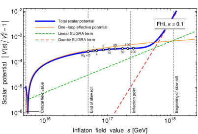
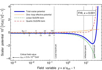
Figure 1: Total scalar potential for the real inflaton field $s$ in F-term hybrid inflation for two representative values of the inflaton Yukawa coupling $\kappa$. Parameter values: (Left panel) $\kappa=10^{-1}$, $\mu_{S}\simeq 1.1\times 10^{15}\,\textrm{GeV}$, $m_{3/2}\simeq 2.7\times 10^{8}\,\textrm{GeV}$ and (Right panel) $\kappa=10^{-3}$, $\mu_{S}\simeq 6.3\times 10^{13}\,\textrm{GeV}$, $m_{3/2}\simeq 6.0\times 10^{3}\,\textrm{GeV}$. Both parameter points are chosen such that they reproduce the measured CMB observables, $A_{s}=A_{s}^{\rm obs}$ and $n_{s}=n_{s}^{\rm obs}$. The left panel represents an example for inflation in the inflection-point regime, while the right panel represents an example for inflation in the hill-top regime. In both plots, we also compare the linear, quartic, and radiative contributions to the total scalar potential.

For $m_{3/2}>m_{3/2}^{\rm crit}$, the potential gradient at the inflection point is negative, $V^{\prime}\left(s_{\rm flex}\right)<0$. This results in the occurrence of a local maximum and a local minimum in the potential near the inflection point, $s_{\rm max}<s_{\rm flex}<s_{\rm min}$. Conversely, for $m_{3/2}<m_{3/2}^{\rm crit}$, the potential gradient at the inflection point is positive, $V^{\prime}\left(s_{\rm flex}\right)>0$. In this case, the potential is monotonically increasing without any local extrema in the vicinity of $s_{\rm flex}$. To distinguish between these two regimes, i.e., the hill-top regime and the inflection-point regime, it is convenient to introduce the following dimensionless parameter,

$$\zeta=\bigg{(}\frac{m_{3/2}^{\rm crit}}{m_{3/2}}\bigg{)}^{2}=\left(\frac{\kappa}{\sqrt{3}\,\pi}\right)^{3}\left(\frac{\mu_{S}^{2}}{4\,m_{3/2}\,M_{\rm Pl}}\right)^{2}\,.$$ (44)

The hill-top and inflection-point regimes then correspond to $\zeta<1$ and $\zeta\geq 1$, respectively. Both regimes are suitable for inflation. In the hill-top regime, inflation can occur near $s_{\rm max}$, while in the inflection-point regime, it can occur near $s_{\rm flex}$ if the potential is sufficiently flat. The parameter $\zeta$ also allows us to write down compact expressions for $s_{\rm max}$ and $s_{\rm min}$ in the hill-top regime,

$$s_{\rm max}=F_{-}\left(\zeta\right)s_{\rm flex}\,,\quad s_{\rm min}=F_{+}\left(\zeta\right)s_{\rm flex}\,,$$ (45)

where $F_{+}$ and $F_{-}$ are complicated functions that correspond to the roots of a quartic polynomial,

$$F_{\pm}\left(\zeta\right)=A^{1/2}\pm\left[\left(\zeta A\right)^{-1/2}-A\right]^{1/2}\,,\quad A=\frac{B_{+}^{2}+B_{-}^{2}}{2\,B_{+}\,B_{-}}\,,\quad B_{\pm}=\left[1\pm\left(1-\zeta^{2}\right)^{1/2}\right]^{1/6}\,.$$ (46)

If inflation occurs at $s\lesssim s_{\rm max}$, the quartic term in Eq. (40) is typically subdominant. This allows us to expand $s_{\rm max}$ in Eq. (45) for small values of $\zeta$. Up to corrections of $\mathcal{O}\left(\zeta^{5/2}\right)$, this results in

$$s_{\rm max}\simeq\frac{3}{4}\,\zeta^{1/2}\,s_{\rm flex}=-\frac{V_{1\ell}^{0}}{c_{s}}=\frac{\kappa^{2}}{16\sqrt{2}\,\pi^{2}}\frac{\mu_{S}^{2}}{m_{3/2}}\,,$$ (47)

which coincides with the result that one obtains if one sets $\lambda_{s}\rightarrow 0$ in Eq. (40) from the outset.

Next, after these remarks on the potential, let us compute the slow-roll parameters $\varepsilon$ and $\eta$,

$$\varepsilon=\frac{M_{\rm Pl}^{2}}{2}\left(\frac{V^{\prime}}{V}\right)^{2}\,,\quad\eta=M_{\rm Pl}^{2}\,\frac{V^{\prime\prime}}{V}\,,\quad V^{\prime}=\frac{\partial V}{\partial s}\,,\quad V^{\prime\prime}=\frac{\partial^{2}V}{\partial s^{2}}\,.$$ (48)

For simplicity, we shall work in the $\lambda_{s}\rightarrow 0$ limit from now on, which will yield acceptable results as long as $\zeta\lesssim\mathcal{O}\left(1\right)$. In fact, we will justify the small-$\lambda_{s}$ approximation a posteriori by an explicit numerical analysis that demonstrates the validity of our analytical results. For small $\lambda_{s}$, we obtain

$$\varepsilon=\frac{1}{2}\left(\frac{c_{s}s+V_{1\ell}^{0}}{V_{F}^{0}}\right)^{2}\left(\frac{M_{\rm Pl}}{s}\right)^{2}\,,\quad\eta=-\frac{V_{1\ell}^{0}}{V_{F}^{0}}\left(\frac{M_{\rm Pl}}{s}\right)^{2}\,.$$ (49)

Note that $\varepsilon$ is suppressed by a factor $V_{1\ell}^{0}/V_{F}^{0}$ compared to $\eta$. As usual in supersymmetric hybrid inflation, the duration of inflation is therefore controlled by $\eta$ — slow-roll inflation only occurs as long as $\eta$ is small. To make this statement more precise, let us impose the following condition on $\eta$,

$$\left|\eta\right|\lesssim\eta_{\rm max}=10^{-0.5}\,.$$ (50)

The transition between slow-roll inflation and the subsequent fast-roll stage is therefore reached at

$$s_{\rm fast}=\left(\frac{V_{1\ell}^{0}}{m_{\rm max}^{2}}\right)^{1/2}=\frac{\kappa\,M_{\rm Pl}}{2\sqrt{2}\,\pi\,\eta_{\rm max}^{1/2}}\,,\quad m_{\rm max}^{2}=\eta_{\rm max}\,\frac{V_{F}^{0}}{M_{\rm Pl}^{2}}\,.$$ (51)

At this field value, $\left|\eta\right|$ saturates the upper bound in Eq. (50). The mass parameter $m_{\rm max}^{2}$ in Eq. (51) denotes the maximal curvature of the potential, $V^{\prime\prime}$, that is allowed by the upper bound on $\eta$. Given the expression for $s_{\rm fast}$ in Eq. (51), we are now able to determine the end point of inflation. Slow-roll inflation either ceases once the inflaton field enters the fast-roll regime (i.e., at $s=s_{\rm fast}$) or once it reaches the critical point in field space that triggers the waterfall transition (i.e., at $s=s_{\rm crit}$),

$$s_{\rm end}=\max\left\{s_{\rm fast},s_{\rm crit}\right\}\,.$$ (52)

The slow-roll parameters in Eq. (49) also allow us to compute the inflationary CMB observables,

$$A_{s}=\frac{1}{24\,\pi^{2}}\frac{V}{\varepsilon\,M_{\rm Pl}^{4}}\,,\quad n_{s}=1+2\,\eta-6\,\varepsilon\,,$$ (53)

where $A_{s}$ and $n_{s}$ denote the amplitude and the spectral index of the scalar power spectrum, respectively. An important step in our analysis will be to identify the parameter regions that manage to reproduce the measured values of these observables. According to the PLANCK 2015 data [67],

$$A_{s}^{\rm obs}\simeq 2.2\times 10^{-9}\,,\quad n_{s}^{\rm obs}\simeq 0.9645\quad\textrm{(TT,\,TE,\,EE\,$+$\,lowP)}\,.$$ (54)

We will not be interested in the tensor-to-scalar ratio $r$. This observable is predicted to be unobservably small in the entire parameter space of interest (see the discussion related to Eq. (17)). The expressions in Eq. (53) can be used to compute theoretical predictions for $A_{s}$ and $n_{s}$. To this end, the slow-roll parameters $\varepsilon$ and $\eta$ need to be evaluated at $s=s_{*}$, i.e., at the inflaton field value that corresponds to the horizon exit of the CMB pivot scale $N_{*}$ $e$-folds before the end of inflation,

$$N_{*}\simeq 47.4+\frac{1}{3}\ln\left(\frac{H_{\rm inf}}{10^{9}\,\textrm{GeV}}\right)+\frac{1}{3}\ln\left(\frac{T_{\rm rh}}{10^{9}\,\textrm{GeV}}\right)\,,$$ (55)

where $T_{\rm rh}$ denotes the reheating temperature after inflation. If not specified otherwise, we will use $T_{\rm rh}\simeq 10^{9}\,\textrm{GeV}$ as a benchmark in the following, which is motivated by thermal leptogenesis [121].

The dynamics of the inflaton field are governed by the following slow-roll equation of motion,

$$s^{\prime}=\Delta\left(\frac{s_{0}}{s}-1\right)s_{0}\,,\quad s^{\prime}=\frac{ds}{N_{e}}\,,\quad s_{0}=-\frac{V_{1\ell}^{0}}{c_{s}}\,.$$ (56)

Here, $s^{\prime}$ stands for the derivative of the inflaton field $s$ w.r.t. the number of $e$-folds $N_{e}$ until the end of inflation. The reference field value $s_{0}$ corresponds to the (would-be) position of the local maximum in the scalar potential. That is, $s_{0}$ is defined through the relation $s_{0}=-V_{1\ell}^{0}/c_{s}$, which coincides with $s_{\rm max}$ in the hill-top regime (i.e., for $\zeta<1$). The parameter $\Delta$ in Eq. (56) measures the strength of the linear SUGRA term in the scalar potential in relation to the radiative corrections,

$$\Delta=\frac{c_{s}^{2}M_{\rm Pl}^{2}}{V_{1\ell}^{0}V_{F}^{0}}=\frac{1}{3}\left(\frac{8\pi}{\kappa}\right)^{2}\left(\frac{m_{3/2}}{H_{\rm inf}}\right)^{2}\,.$$ (57)

Given the boundary condition that the field $s$ must reach $s_{\rm end}$ for $N_{e}=0$, Eq. (56) has a unique solution in terms of the (principal branch of the) Lambert W function or product logarithm $W_{0}$,

$$s\left(N_{e}\right)=s_{0}\left(1+W\right)\,,\quad W=W_{0}\left[\left(\frac{s_{\rm end}}{s_{0}}-1\right)\exp\left(\frac{s_{\rm end}}{s_{0}}-1\right)e^{-\Delta\,N_{e}}\right]\,.$$ (58)

$W_{0}$ is the inverse function of the product function $Xe^{X}$ and, thus, features the following properties,

$$X=W_{0}\left(X\right)e^{W_{0}\left(X\right)}\,,\quad W_{0}\left(Xe^{X}\right)=X\,,\quad W_{0}\left(0\right)=0\,,\quad W_{0}\left(X\right)\geq-1\,.$$ (59)

The solution in Eq. (58) can also be written as a function of the three parameters $\eta_{\rm max}$, $N_{e}$, and $\Delta$,

$$s\left(N_{e}\right)=s_{0}\left(1+W\right)\,,\quad W=W_{0}\left(Xe^{X-\Delta\,N_{e}}\right)\,,\quad X=\left(\frac{\Delta}{\eta_{\rm max}}\right)^{1/2}-1\,.$$ (60)

With the aid of Eq. (60), the slow-roll parameters $\varepsilon$ and $\eta$ in Eq. (49) can be written as follows,

$$\varepsilon=\bigg{(}\frac{\kappa}{4\pi}\bigg{)}^{2}\left(\frac{W}{1+W}\right)^{2}\Delta\,,\quad\eta=-\left(\frac{1}{1+W}\right)^{2}\Delta\,.$$ (61)

These explicit expressions illustrate once more that $\varepsilon$ is suppressed by a loop factor compared to $\eta$. In the computation of the scalar spectral index $n_{s}$, we can therefore neglect $\varepsilon$ and simply use

$$n_{s}\approx 1+2\,\eta=1-\frac{2\Delta}{\left(1+W\right)^{2}}\,.$$ (62)

This relation allows us to compute $n_{s}$ as a function of $\eta_{\rm max}$, $N_{e}$, and $\Delta$. Or in other words, for given values of $\eta_{\rm max}$ and $N_{e}$, the measured value $n_{s}^{\rm obs}$ directly translates into a specific value for $\Delta$,

$$\eta_{\rm max}=10^{-0.5}\,,\quad N_{*}=50\,,\quad n_{s}=n_{s}^{\rm obs}\qquad\Rightarrow\qquad\Delta\simeq 7.1\times 10^{-3}\,.$$ (63)

This is an important result that eliminates one free parameter from our analysis. First of all, we note that the numerical values in Eq. (63) fix the field value $s_{*}$ at the time of CMB horizon exit,

$$\eta_{\rm max}=10^{-0.5}\,,\quad N_{*}=50\,,\quad\Delta\simeq 7.1\times 10^{-3}\qquad\Rightarrow\qquad W\simeq-0.37\,,\quad s_{*}\simeq 0.63\,s_{\rm max}\,.$$ (64)

But more importantly, the measured value of $\Delta$ also fixes the relation between $m_{3/2}$ and $H_{\rm inf}$,

$$m_{3/2}=\frac{\kappa}{8\pi}\sqrt{3}\,\Delta^{1/2}H_{\rm inf}\simeq 5.8\times 10^{-4}\,H_{\rm inf}\,\bigg{(}\frac{\kappa}{0.1}\bigg{)}\,.$$ (65)

Evidently, the gravitino mass needs to be several orders of magnitude smaller than the inflationary Hubble rate in order to explain the observed scalar spectral index, $m_{3/2}\ll H_{\rm inf}$. This conclusion justifies our decision to neglect the quadratic mass term in Eq. (40). Moreover, the relation in Eq. (65) also results in a numerical expression for the parameter $\zeta$ as a function of the coupling $\kappa$,

$$\zeta=\frac{4\,\kappa}{3\sqrt{3}\,\pi\,\Delta}\simeq 3.5\,\bigg{(}\frac{\kappa}{0.1}\bigg{)}\,.$$ (66)

For $\kappa\geq 3/4\sqrt{3}\,\pi\,\Delta\simeq 2.9\times 10^{-2}$, inflation therefore occurs in the inflection-point regime, while for smaller $\kappa$ values, it occurs in the hill-top regime. According to Eq. (66), we also expect that our analysis in the small-$\lambda_{s}$ approximation should be reliable as long as $\kappa\lesssim 0.1$, so that $\zeta\lesssim\mathcal{O}\left(1\right)$.

In addition to $n_{s}^{\rm obs}$, we can also use the observed value of the scalar spectral amplitude, $A_{s}^{\rm obs}$, to eliminate yet another parameter from the analysis. Making use of Eqs. (53) and (61), we can write

$$A_{s}=\frac{2}{3\,\kappa^{2}\,\Delta}\left(\frac{1+W}{W}\right)^{2}\left(\frac{\mu_{S}}{M_{\rm Pl}}\right)^{4}\,.$$ (67)

The condition $A_{s}=A_{s}^{\rm obs}$ can then be solved for the inflaton F-term mass scale as a function of $\kappa$,

$$\mu_{S}=\left(\frac{3}{2}\,A_{s}^{\rm obs}\Delta\right)^{1/4}\left(\frac{\kappa\left|W\right|}{1+W}\right)^{1/2}M_{\rm Pl}\simeq 1.3\times 10^{15}\,\textrm{GeV}\>\bigg{(}\frac{\kappa}{0.1}\bigg{)}^{1/2}\,.$$ (68)

This result immediately fixes the SSB scale of the waterfall transition at the end of inflation,

$$v=\left(6\,A_{s}^{\rm obs}\Delta\right)^{1/4}\left(\frac{\left|W\right|}{1+W}\right)^{1/2}M_{\rm Pl}\simeq 5.8\times 10^{15}\,\textrm{GeV}\,,$$ (69)

which is remarkably close to the GUT scale in typical SUSY GUT scenarios, $\Lambda_{\rm GUT}\sim 10^{16}\,\textrm{GeV}$. The numerical result in Eq. (69) therefore serves as another indication that FHI is, indeed, well suited to be embedded into a bigger GUT framework. Eq. (69) also fixes the cosmic string tension,

$$G\,\mu_{\rm CS}=\left(\frac{3}{8}\,A_{s}^{\rm obs}\Delta\right)^{1/2}\frac{\epsilon_{\rm CS}\left|W\right|}{1+W}\simeq 6.4\times 10^{-7}\>\bigg{(}\frac{\epsilon_{\rm CS}}{0.45}\bigg{)}\,,$$ (70)

where we used that $\epsilon_{\rm CS}\simeq 0.45$ for $\kappa=10^{-1}$ (see Eqs. (36) and (37)). In view of Eq. (70), we conclude that FHI in the large-$\kappa$ regime produces cosmic strings with a large tension that is conflict with the observational bound in Eq. (33). Therefore, if we take the bound in Eq. (33) seriously, FHI in the large-$\kappa$ regime is ruled out. Alternatively, we can simply presume that the gauge symmetry $G$ already becomes broken in a different sector before the end of inflation. In this case, we do not need to worry about the large cosmic string tension in Eq. (70) (see the discussion below Eq. (38)).

In consequence of the two conditions $n_{s}=n_{s}^{\rm obs}$ and $A_{s}=A_{s}^{\rm obs}$, the viable parameter space of FHI shrinks to a one-dimensional hypersurface that can be parametrized in terms of the Yukawa coupling $\kappa$. The Hubble rate $H_{\rm inf}$, e.g., follows immediately from the expression for $\mu_{S}$ in Eq. (68),

$$H_{\rm inf}=\left(\frac{1}{2}\,A_{s}^{\rm obs}\Delta\right)^{1/2}\frac{\kappa\left|W\right|}{1+W}\,M_{\rm Pl}\simeq 4.0\times 10^{11}\,\textrm{GeV}\>\bigg{(}\frac{\kappa}{0.1}\bigg{)}\,.$$ (71)

Thanks to the relation in Eq. (65), this result for $H_{\rm inf}$ determines in turn the gravitino mass $m_{3/2}$,

$$m_{3/2}=\left(\frac{3}{2}\,A_{s}^{\rm obs}\right)^{1/2}\frac{\kappa^{2}}{8\pi}\frac{\Delta\left|W\right|}{1+W}\,M_{\rm Pl}\simeq 2.3\times 10^{8}\,\textrm{GeV}\>\bigg{(}\frac{\kappa}{0.1}\bigg{)}^{2}\,.$$ (72)

At this point, we emphasize that Eq. (72) corresponds to the solution for $m_{3/2}$ on the negative real axis. As shown in [102], more complicated trajectories in the complex inflaton plane also lead to successful inflation — however, keeping the value of $H_{\rm inf}$ fixed, these alternative solutions are all associated with a larger value of $m_{3/2}$. In this sense, the expression in Eq. (72) should be regarded as a lower bound on the gravitino mass in FHI (see the discussion below Eq. (28)). Furthermore, given the $\kappa$ dependence of $\mu_{S}$ and $m_{3/2}$ in Eqs. (68) and (72), we are now able to compute the critical $\kappa$ value that separates the large-$\kappa$ regime (where $x_{*}\gg 1$) from the small-$\kappa$ regime (where $x_{*}\simeq 1$),

$$s_{\rm scrit}=s_{\rm max}\qquad\Rightarrow\qquad\kappa_{0}=4\left[\pi^{2}\,\frac{m_{3/2}\left(\kappa_{0}\right)}{\mu_{S}\left(\kappa_{0}\right)}\right]^{2/5}\simeq 1.8\times 10^{-3}\,.$$ (73)

As anticipated at the beginning of this section, the critical $\kappa$ value is, indeed, of $\mathcal{O}\left(10^{-3}\right)$.

The expressions for $H_{\rm inf}$ and $m_{3/2}$ in Eqs. (71) and (72) mark the main technical results in this section. Based on these results, we can now determine the implications of the CDM isocurvature constraint on the parameters of FHI in the large-$\kappa$ regime. Confronting our explicit expression for $H_{\rm inf}$ in Eq. (71) with the upper bound in Eq. (15), we arrive at the following upper bound on $\kappa$,

$$\boxed{\kappa\lesssim 3.1\times 10^{-3}\left(\frac{1}{F_{\rm DM}^{a}}\right)^{1/2}\left(\frac{f_{a}}{M_{\rm Pl}}\right)^{0.42}}$$ (74)

This is a tight constraint on the inflaton Yukawa coupling $\kappa$. In fact, only for a very large axion decay constant, $f_{a}\sim M_{\rm Pl}$, the bound in Eq. (74) manages to exceed the critical $\kappa$ value in Eq. (73). In view of this result, it is important to remember that a Planck-scale axion decay constant is questionable for both theoretical and phenomenological reasons. On the one hand, string theory suggests that it is impossible to realize an axion decay constant larger than the Planck scale. Values as large as $f\sim M_{\rm Pl}$ are therefore only marginally feasible. Instead, string theory rather points to axion decay constants of the order of $f_{a}\sim 10^{16}\cdots 10^{17}\,\textrm{GeV}$ [122, 123, 124]. On the other hand, spin measurements of stellar black holes allow to constrain $f_{a}$ based on the phenomenon of black hole superradiance. At present, these measurements exclude $f_{a}$ values in the range $3\times 10^{17}\,\textrm{GeV}\lesssim f_{a}\lesssim 10^{19}\,\textrm{GeV}$ [123, 125, 126]. We, thus, conclude that FHI in the large-$\kappa$ regime is highly constrained by the CDM isocurvature bound. A viable region in parameter space survives only if $f_{a}\sim M_{\rm Pl}$ for one reason or another. Making use of Eq. (72), the bound in Eq. (74) can also be formulated as an upper bound on $m_{3/2}$,

$$\boxed{m_{3/2}\lesssim 2.2\times 10^{5}\,\textrm{GeV}\left(\frac{1}{F_{\rm DM}^{a}}\right)\left(\frac{f_{a}}{M_{\rm Pl}}\right)^{0.83}}$$ (75)

Again, we stress that this is an inclusive upper bound on $m_{3/2}$ that guarantees that the CDM isocurvature constraint in Eq. (15) is satisfied, no matter which inflationary trajectory is chosen in the complex inflaton plane. A more extensive analysis assessing the dependence on the chosen trajectory is much more involved and beyond the scope of this work. In Fig. 2, we show the upper bounds on $\mu_{S}$, $m_{3/2}$, etc. for a few representative values of $f_{a}$. The plots in Fig. 2 are based on a fully numerical analysis of slow-roll inflation in the complete scalar potential of FHI (see Eqs. (24) and (31)). The comparison between these plots and the analytical results derived in this section demonstrates that our analytical calculations reproduce the exact results very well. This observation serves as a cross-check and validates the various approximations in the above discussion.

Finally, we use the expression for $H_{\rm inf}$ in Eq. (71) to determine the parameter region in which the PQ symmetry actually remains intact during inflation. In this case, the requirement $H_{\rm inf}>f_{a}$ results in lower bounds on the Yukawa coupling $\kappa$ and the gravitino mass $m_{3/2}$,

$$\kappa\gtrsim 2.5\times 10^{-3}\left(\frac{f_{a}}{10^{10}\,\textrm{GeV}}\right)\,,\quad m_{3/2}\gtrsim 1.5\times 10^{5}\,\textrm{GeV}\left(\frac{f_{a}}{10^{10}\,\textrm{GeV}}\right)^{2}\,.$$ (76)

Thus, for low values of the axion decay constant, $f_{a}\sim 10^{10}\,\textrm{GeV}$, the PQ symmetry is only spontaneously broken after inflation, which may result in the production of dangerous domain walls.

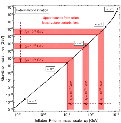
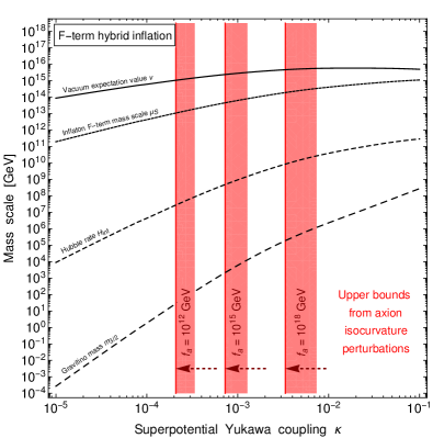
Figure 2: Parameter values for F-term hybrid inflation that reproduce the CMB data, $A_{s}=A_{s}^{\rm obs}$ and $n_{s}=n_{s}^{\rm obs}$, in combination with the CDM isocurvature constraint for several values of the axion decay constant and different assumptions regarding the axion DM fraction. The stronger [weaker] bounds correspond to $F_{\rm DM}^{a}=1$ [$F_{\rm DM}^{a}=0.1$]. (Left panel) One-dimensional hypersurface in the $\mu_{S}$–$m_{3/2}$ plane that manages to reproduce the observed CMB data. (Right panel) Various mass scales that are relevant in the description of FHI as functions of the Yukawa coupling $\kappa$. Both plots are based on a numerical analysis that accounts for the complete scalar potential in Eqs. (24) and (31).

3.3 Inflation close to the waterfall phase transition

In the previous section, we saw that FHI in the large-$\kappa$ regime is highly constrained by the nonobservation of axion isocurvature perturbations and the upper bound on the cosmic string tension. This situation changes in the small-$\kappa$ regime, which opens up the possibility to lower the inflationary Hubble scale to smaller values, $H_{\rm inf}\lesssim\mathcal{O}\left(10^{9}\right)\,\textrm{GeV}$. This scenario is therefore compatible with values of the axion decay constant significantly below the Planck scale, $f_{a}\ll M_{\rm Pl}$. However, it is clear from the outset that this improvement over the large-$\kappa$ regime is not for free. The price one has to pay is an additional tuning in the initial conditions of inflation. In the small-$\kappa$ regime, the local maximum in the scalar potential is located in the direct vicinity of the critical field value that triggers the waterfall transition. The initial field value $s_{\rm ini}$, thus, has to be tuned to lie in the small interval in between $s_{\rm crit}$ and $s_{\rm max}$ to ensure that inflation proceeds in the correct direction in field space. Otherwise, i.e., for $s_{\rm ini}>s_{\rm max}$, the inflaton will roll towards the false vacuum at $s=s_{\rm min}$, so that inflation never ends (see the right panel of Fig. 1). On the other hand, we stress that a fine-tuning of the initial conditions is of a different conceptual quality than a fine-tuning of model parameters. One may, e.g., speculate that the evolution of the inflaton field prior to inflation is responsible for a dynamical selection of initial field values close to $s_{\rm max}$ for one reason or another. In addition, as shown in [102], the issue of initial conditions in FHI becomes relaxed if one accounts for all possible trajectories in the complex plane. In this case, it is possible that the inflaton trajectory starts out at large field values and then bends in just the right way to avoid the local minimum at $s=s_{\rm min}$. Finally, we point out that the small-$\kappa$ regime does not require any unnatural fine-tuning of model parameters. In the $\kappa\rightarrow 0$ limit, the waterfall fields cease to participate in Yukawa interactions. This restores a global $U(1)\times U(1)$ symmetry in the waterfall sector that contains the local gauge symmetry $G$ as a subgroup. Small $\kappa$ values are therefore natural in the sense of ’t Hooft [127].

In the small-$\kappa$ regime, we can no longer use the large-field expansion of the loop function $L$ in Eq. (39). Instead, we now have to evaluate $L$ in the vicinity of the critical field value $s_{\rm crit}$,

$$L\left(x\right)=L_{2}\left(y\right)+\mathcal{O}\left(y^{3}\right)\,,\quad x=\left(\frac{s}{s_{\rm crit}}\right)^{2}\,,\quad y=\frac{s}{s_{\rm crit}}-1\,.$$ (77)

Here, $L_{2}$ encompasses the leading contributions to $L$ up to second order in the new field variable $y$,

$$L_{2}\left(y\right)=c_{0}+c_{1}\,y+\frac{1}{2}\left(c_{2}+\bar{c}_{2}\ln y\right)y^{2}\,.$$ (78)

The coefficients $c_{0}$, $c_{1}$, $c_{2}$, and $\bar{c}_{2}$ can be determined analytically,

$$c_{0}=2\ln 2-\frac{3}{2}\,,\quad c_{1}=4\ln 2\,,\quad c_{2}=6\left(2\ln 2-1\right)\,,\quad\bar{c}_{2}=4\,.$$ (79)

Given this expansion of the radiative one-loop corrections, the inflaton potential now reads

$$V\simeq V_{F}^{0}+c_{s}\,s+\frac{1}{2}\,V_{1l}^{0}\,L_{2}\left(y\right)\,,$$ (80)

where we again neglected the quartic SUGRA term. Correspondingly, $\varepsilon$ and $\eta$ in Eq. (49) turn into

$$\varepsilon=\frac{1}{2}\left(\frac{c_{s}s_{\rm crit}+c_{1}V_{1\ell}^{0}/2}{V_{F}^{0}}\right)^{2}\left(\frac{M_{\rm Pl}}{s_{\rm crit}}\right)^{2}\,,\quad\eta=\frac{V_{1\ell}^{0}}{2\,V_{F}^{0}}\left(c_{2}+\frac{3}{2}\,\bar{c}_{2}+\bar{c}_{2}\ln y\right)\left(\frac{M_{\rm Pl}}{s_{\rm crit}}\right)^{2}\,.$$ (81)

Also the slow-roll equation of motion in Eq. (56) obtains a new form. To leading order, we can write

$$s^{\prime}=\sqrt{2}\,\varepsilon^{1/2}M_{\rm Pl}\,.$$ (82)

This equation can be readily integrated, resulting in the following expression for the inflaton field $s$,

$$s\left(N_{e}\right)=s_{\rm crit}+\sqrt{2}\,\varepsilon^{1/2}M_{\rm Pl}\,N_{e}\,.$$ (83)

As before, we shall now eliminate two free parameters by making use of the conditions $A_{s}=A_{s}^{\rm obs}$ and $n_{s}=n_{s}^{\rm obs}$. To this end, we first solve $A_{s}=A_{s}^{\rm obs}$ for the slow-roll parameter $\varepsilon$ (see Eq. (53)),

$$\varepsilon=\frac{1}{24\pi^{2}}\frac{V_{F}^{0}}{A_{s}^{\rm obs}M_{\rm Pl}^{4}}\,.$$ (84)

Then, we equate this result with the expression for $\varepsilon$ in Eq. (81) and solve for the gravitino mass,

$$m_{3/2}=\left[\ln 2\,\kappa^{5/2}-\frac{2\sqrt{2}\,\pi}{\sqrt{3}\left(A_{s}^{\rm obs}\right)^{1/2}}\left(\frac{\mu_{S}}{M_{\rm Pl}}\right)^{3}\right]\frac{\mu_{S}}{16\pi^{2}}\,.$$ (85)

Next, we make use of the condition $n_{s}=n_{s}^{\rm obs}$. Again, we approximate $n_{s}\approx 1+2\,\eta$, such that

$$n_{s}\approx 1+2\,\ln\left(8y_{*}\right)\delta\,.$$ (86)

Here, the dimensionless parameter $\delta$ characterizes the curvature of $V_{1\ell}$ close to the critical field value,

$$\delta=\frac{2V_{1\ell}^{0}}{V_{F}^{0}}\left(\frac{M_{\rm Pl}}{s_{\rm crit}}\right)^{2}=\frac{\kappa^{3}}{8\pi^{2}}\left(\frac{M_{\rm Pl}}{\mu_{S}}\right)^{2}\,.$$ (87)

Meanwhile, $y_{*}$ stands for the field variable $y$ evaluated at the time of CMB horizon exit,

$$y_{*}=\frac{s_{*}}{s_{\rm crit}}-1=\sqrt{2}\,\varepsilon^{1/2}N_{*}\,\frac{M_{\rm Pl}}{s_{\rm crit}}=\frac{\kappa^{2}}{8\sqrt{3}\,\pi^{2}}\frac{N_{*}}{\left(A_{s}^{\rm obs}\delta\right)^{1/2}}\,.$$ (88)

Putting everything together, we find that the scalar spectral index can be written as follows,

$$n_{s}=1-\ln\left(\frac{3\pi^{4}}{\kappa^{4}}\frac{A_{s}^{\rm obs}}{N_{*}^{2}}\,\delta\right)\delta\,.$$ (89)

In the next step, we explicitly solve the condition $n_{s}=n_{s}^{\rm obs}$ for the curvature parameter $\delta$,

$$\delta=\frac{1-n_{s}^{\rm obs}}{W_{0}\left(Y\right)}\,,\quad Y=\left(1-n_{s}^{\rm obs}\right)\frac{3\pi^{4}}{\kappa^{4}}\frac{A_{s}^{\rm obs}}{N_{*}^{2}}\,,$$ (90)

where $W_{0}$ again denotes the Lambert W function (see Eq. (59)). The result in Eq. (90) enables us to compute $\delta$ as a function of $N_{*}$ and $\kappa$. For $N_{*}=47.5$ and $\kappa=10^{-5}$, we find, e.g., $\delta\simeq 0.002$. The dependence of $\delta$ on the Yukawa coupling $\kappa$ is in general rather weak. For $\kappa$ values in between $10^{-7}$ and $10^{-3}$, the parameter $\delta$ varies only by roughly an order of magnitude, $0.001\lesssim\delta\lesssim 0.02$.

The definition of $\delta$ in Eq. (87) can be solved for the inflaton F-term mass scale. We, thus, obtain

$$\mu_{S}=\left(\frac{\kappa^{3}}{8\pi^{2}\delta}\right)^{1/2}M_{\rm Pl}\simeq 1.9\times 10^{11}\,\textrm{GeV}\left(\frac{0.002}{\delta}\right)^{1/2}\bigg{(}\frac{\kappa}{10^{-5}}\bigg{)}^{3/2}\,.$$ (91)

Again, this result immediately translates into an expression for the SSB scale $v$,

$$v=\frac{\kappa\,M_{\rm Pl}}{2\pi\,\delta^{1/2}}\simeq 8.7\times 10^{13}\,\textrm{GeV}\left(\frac{0.002}{\delta}\right)^{1/2}\bigg{(}\frac{\kappa}{10^{-5}}\bigg{)}\,,$$ (92)

which now turns out to be parametrically suppressed compared to the GUT scale, $\Lambda_{\rm GUT}\sim 10^{16}\,\textrm{GeV}$. Unlike Eq. (69), Eq. (92) results in a parameter-dependent expression for the cosmic string tension,

$$G\,\mu_{\rm CS}=\bigg{(}\frac{\kappa}{4\pi}\bigg{)}^{2}\>\frac{\epsilon_{\rm CS}}{\delta}\simeq 3.2\times 10^{-11}\left(\frac{0.002}{\delta}\right)\bigg{(}\frac{\kappa}{10^{-5}}\bigg{)}^{2}\bigg{(}\frac{\epsilon_{\rm CS}}{0.10}\bigg{)}\,,$$ (93)

where we used that $\epsilon_{\rm CS}\simeq 0.10$ for $\kappa=10^{-5}$ (see Eqs. (36) and (37)). Therefore, for a sufficiently small value of the Yukawa coupling $\kappa$, there is no problem to satisfy the bound on the cosmic string tension in Eq. (33). As mentioned above, the only price to pay is an increased tuning in the initial conditions for inflation. Eq. (91) also results in an expression for the inflationary Hubble rate,

$$H_{\rm inf}=\frac{\kappa^{3}\,M_{\rm Pl}}{8\sqrt{3}\,\pi^{2}\delta}\simeq 9.0\times 10^{3}\,\textrm{GeV}\left(\frac{0.002}{\delta}\right)\bigg{(}\frac{\kappa}{10^{-5}}\bigg{)}^{3}\,,$$ (94)

which now scales more strongly with $\kappa$ than in the large-$\kappa$ regime (see Eq. (71)). Similarly, we can use the results in Eqs. (85) and (91) to obtain an expression for $m_{3/2}$ as a function of $\kappa$,

$$m_{3/2}=\left[\ln 2-\frac{\kappa^{2}}{8\sqrt{3}\,\pi^{2}\left(A_{s}^{\rm obs}\right)^{1/2}\delta^{3/2}}\right]\frac{\kappa^{4}M_{\rm Pl}}{32\sqrt{2}\,\pi^{3}\,\delta^{1/2}}\,.$$ (95)

For small $\kappa$, the $\ln 2$ term dominates the square brackets on the RHS of this expression, such that

$$m_{3/2}\approx\frac{\ln 2\,\kappa^{4}M_{\rm Pl}}{32\sqrt{2}\,\pi^{3}\,\delta^{1/2}}\simeq 2.7\times 10^{-4}\,\textrm{GeV}\left(\frac{0.002}{\delta}\right)^{1/2}\bigg{(}\frac{\kappa}{10^{-5}}\bigg{)}^{4}\,.$$ (96)

With the above results at hand, we can again use the CDM isocurvature bound in Eq. (15) to constrain the parameter space of FHI. However, this time, we need to determine all bounds numerically because of the complicated $\kappa$ dependence of the parameter $\delta$ (see Eq. (90)). First, we compare our result for $H_{\rm inf}$ in Eq. (94) with Eq. (15) to determine an upper bound on $\kappa$,

$$\boxed{\kappa\lesssim 1.0\times 10^{-3}\left(\frac{1}{F_{\rm DM}^{a}}\right)^{0.21}\left(\frac{f_{a}}{10^{16}\,\textrm{GeV}}\right)^{0.17}}$$ (97)

This constraint is consistent with the critical $\kappa$ value in Eq. (73) that separates the small-$\kappa$ regime from the large-$\kappa$ regime. In particular, as we are working with small values of $\kappa$ in this section, the axion decay constant $f_{a}$ can now be chosen to be significantly smaller than the Planck scale. Combining our results in Eqs. (96) and (97), we are also able to deduce an upper bound on $m_{3/2}$,

$$\boxed{m_{3/2}\lesssim 9.4\times 10^{3}\,\textrm{GeV}\left(\frac{1}{F_{\rm DM}^{a}}\right)^{0.76}\left(\frac{f_{a}}{10^{16}\,\textrm{GeV}}\right)^{0.63}}$$ (98)

Just like the bound in Eq. (75), this bound is again an absolute upper bound that guarantees that the CDM isocurvature constraint is satisfied for all possible trajectories in the complex plane. The (quasi-) analytical result in Eq. (98) needs to be compared to the fully numerical result in Fig. 2. Again, we find excellent agreement, which confirms the validity of the above analytical discussion. Eq. (96) can also be used to translate the upper bound on the cosmic string tension in Eq. (33) into an upper bound on the gravitino mass. The combination of Eqs. (33), (93), and (96) results in

$$G\,\mu_{\rm CS}<G\,\mu_{\rm CS}^{\rm max}\qquad\Rightarrow\qquad\kappa\lesssim 1.8\times 10^{-3}\,,\quad m_{3/2}\lesssim 3.2\times 10^{4}\,\textrm{GeV}\,.$$ (99)

where we used that $\epsilon_{\rm CS}\simeq 0.18$ for $\kappa=1.8\times 10^{-3}$ (see Eqs. (36) and (37)). Note that the upper bound on $\kappa$ accidentally coincides with the critical $\kappa$ value in Eq. (73). By coincidence, the region in parameter space where $G\,\mu_{\rm CS}<G\,\mu_{\rm CS}^{\rm max}$ therefore happens to be identical with the small-$\kappa$ regime. Thanks to Eqs. (91), (92), and (94), the bounds in Eq. (99) also result in the following constraints,

$$v\lesssim 3.6\times 10^{15}\,\textrm{GeV}\,,\quad\mu_{S}\lesssim 1.1\times 10^{14}\,\textrm{GeV}\,,\quad H_{\rm inf}\lesssim 2.8\times 10^{9}\,\textrm{GeV}\,.$$ (100)

This result is consistent with the bound on the SSB scale $v$ in Eq. (38).

Finally, similarly to the large-$\kappa$ case, we conclude by determining the region in parameter space where the PQ symmetry remains intact during inflation. Combining Eqs. (94) and (96) with the requirement that $H_{\rm inf}$ must exceed $f_{a}$, we obtain the following lower bounds on $\kappa$ and $m_{3/2}$,

$$\kappa\gtrsim 3.4\times 10^{-4}\left(\frac{f_{a}}{10^{8}\,\textrm{GeV}}\right)^{0.39}\,,\quad m_{3/2}\gtrsim 1.8\times 10^{2}\,\textrm{GeV}\left(\frac{f_{a}}{10^{8}\,\textrm{GeV}}\right)^{1.47}\,.$$ (101)

Thus, for small values of the axion decay constant $f_{a}$, there are also viable parameter combinations in the small-$\kappa$ regime that are compatible with the postinflationary PQSB scenario.

4 Low-scale D-term hybrid inflation

4.1 Model setup and scalar potential

In Sec. 3, we discussed the slow-roll dynamics of FHI and the compatibility with the CDM isocurvature constraint in Eq. (15). We found an absolute upper bound on the Yukawa coupling $\kappa$ of $\mathcal{O}\left(10^{-3}\right)$ (see Eq. (74)) and a corresponding bound on the gravitino mass $m_{3/2}$ of $\mathcal{O}\left(10^{5}\right)\,\textrm{GeV}$ (see Eq. (75)). Moreover, we concluded that the large-$\kappa$ regime of FHI is strongly constrained by the nonobservation of axion isocurvature perturbations and the upper bound on the cosmic string tension. Likewise, we concluded that the small-$\kappa$ regime of FHI manages to avoid these constraints — however, at the price of a moderate fine-tuning of the initial conditions of inflation. In addition, we recall that both regimes of FHI actually need to be described as a two-field model of inflation. As shown in [102], this includes the possibility of inflaton trajectories in the complex plane that fail to reach the critical field value $s_{\rm crit}$. FHI therefore requires an additional selection mechanism among all possible trajectories ensuring that inflaton ends in a successful waterfall transition.

In this section, we will now show that most of the above problems related to FHI are absent in the case of DHI. The reason for this is twofold: First of all, DHI is a standard single-field model of inflation. The inflaton field does not possess an F term and, hence, the rotational invariance in the complex plane remains unbroken. Thus, there are no problems related to the proper choice of trajectory in field space. Second, in contrast to FHI, the dynamics of DHI are controlled by the magnitude of the gauge coupling constant $g$. This provides a larger parametric freedom that can be used to achieve a low Hubble rate even in the large-$\kappa$ regime. In DHI, it is therefore possible to satisfy the CDM isocurvature constraint without any fine-tuning of the initial conditions. Only the issue of cosmic string formation during the waterfall transitions remains more or less unaffected. Also in DHI, the cosmic string tension can only be successfully suppressed if the inflaton Yukawa coupling $\kappa$ is set to a small value, $\kappa\lesssim\mathcal{O}\left(10^{-4}\right)$. However, we reiterate that this constraint becomes null if cosmic strings already form before the end of inflation (see the discussion below Eq. (38)).

We begin by describing the setup of our model and collecting a few important properties of the scalar potential. Again, we will incorporate the effect of spontaneous SUSY breaking in the form of a hidden Polonyi sector that couples to the inflaton sector only via gravitational interactions. The superpotential of our model, thus, follows from Eq. (19) after setting the inflaton F-term mass scale to zero, $\mu_{S}\rightarrow 0$. The Kähler potential remains unchanged and is the same as in FHI (see Eq. (20)),

$$W=\kappa\,S\,\Phi\bar{\Phi}+\mu_{X}^{2}X+w\,,\quad K=S^{\dagger}S+\Phi^{\dagger}\Phi+\bar{\Phi}^{\dagger}\bar{\Phi}+X^{\dagger}X+\frac{\chi}{M_{\rm Pl}^{2}}\,S^{\dagger}S\,X^{\dagger}X+\cdots\,.$$ (102)

We continue to assume that $X$ is safely stabilized at the origin in field space, $\left<X\right>=0$, such that the relations in Eq. (21) remain valid also in the case of DHI. The crucial difference between FHI and DHI is that, instead of an inflaton F term in the superpotential, DHI features a nonvanishing Fayet-Iliopoulos (FI) D term [128]. This results in an FI parameter $\xi$ in the D-term scalar potential,

$$V_{D}=\frac{g^{2}}{2}\left[q_{0}\,\xi-q\left(\left|\phi\right|^{2}-\left|\bar{\phi}\right|^{2}\right)\right]^{2}\,.$$ (103)

For definiteness, we will assume $\xi>0$. The gauge charge $q_{0}$ in front of $\xi$ serves as a rescaling factor that can take different values depending on the dynamical origin of the FI parameter. Without loss of generality, we will simply set $q_{0}=q=1$ in the following. This is possible since the case of general gauge charges $q_{0}$ and $q$ can always be restored by the following reparametrization of $g$ and $\xi$,

$$g\rightarrow g^{\prime}=\frac{g}{q}\,,\quad\xi\rightarrow\xi^{\prime}=\frac{q}{q_{0}}\,\xi\,.$$ (104)

The origin of the FI parameter $\xi$ in Eq. (103) has been the subject of a long debate in the literature. In particular, it has been pointed out that it is not possible to consistently embed a genuine (i.e., constant) FI parameter $\xi$ into SUGRA [129, 130]. Therefore, $\xi$ needs to be an effective FI parameter that depends on the VEVs of scalar moduli. This can, e.g., be achieved in string theory [131, 132] via the Green-Schwarz mechanism of anomaly cancellation [133] or in strongly coupled gauge theories via the effect of dimensional transmutation [134] (see [81, 82] for an explicit DHI model). Besides that, there have recently been various proposals for nonstandard FI terms that can be consistently embedded into SUGRA after all [135, 136] (see [137] for an explicit DHI model). However, in this paper, we will not delve into the details of this issue. Instead, we will simply assume that an appropriate ultraviolet completion — presumably related to one of the mechanisms listed above — results in an effective FI term that can be treated as a constant for the purposes of inflation. Any further speculations regarding the origin of the FI parameter $\xi$ are beyond the scope of this work.

The waterfall fields are again stabilized at zero during inflation, $\big{<}\Phi\big{>}=\big{<}\bar{\Phi}\big{>}=0$. However, in DHI, only one field obtains a VEV during the waterfall transition. Given our sign conventions,

$$\big{<}\Phi\big{>}=\frac{v}{\sqrt{2}}\,,\quad\big{<}\bar{\Phi}\big{>}=0\,,\quad v=\sqrt{2\,\xi}\,,$$ (105)

where $v$ is again normalized such that it corresponds to the VEV of the real Higgs scalar contained in $\Phi$. The F-term scalar potential of DHI simply follows from setting $\mu_{S}\rightarrow 0$ in Eq. (24),

$$V_{F}=e^{z}\,\frac{1-\chi\left(3-z\right)}{2\left(1+\chi\,z\right)}\,m_{3/2}^{2}\,s^{2}\,,\quad z=\frac{s^{2}}{2\,M_{\rm Pl}^{2}}\,.$$ (106)

The disappearance of the inflaton F term also eliminates the dependence on the complex inflaton phase $\varphi$. DHI is therefore, indeed, a single-field model that preserves the rotational invariance in the complex inflaton plane. Moreover, the F-term scalar potential in Eq. (106) no longer contains odd powers of the real inflaton field $s$. Most notably, the linear tadpole term that is crucial for the dynamics of FHI (see Eq. (28)) is now absent. The only terms that survive at small field values are the quadratic mass term and the quartic self-interaction. Analogously to Eq. (26), we can write

$$V_{F}=\frac{1}{2}\,m_{s}^{2}\,s^{2}+\frac{1}{24}\,\lambda_{s}\,s^{4}+\mathcal{O}\left(s^{6}\right)\,,$$ (107)

where the coefficients $m_{s}^{2}$ and $\lambda_{s}$ are identical to the expressions in Eq. (29) in the limit $\mu_{S}\rightarrow 0$,

$$m_{s}^{2}=\left(1-3\chi\right)m_{3/2}^{2}\,,\quad\lambda_{s}=6\left(1-3\chi+3\chi^{2}\right)\left(\frac{m_{3/2}}{M_{\rm Pl}}\right)^{2}\,.$$ (108)

Evidently, the mass squared $m_{s}^{2}$ remains unchanged, while the quartic self-coupling constant $\lambda_{s}$ no longer receives a contribution from the superpotential in the inflation sector. DHI only manages to reproduce the correct scalar spectral index, $n_{s}=n_{s}^{\rm obs}$, if the F-term scalar potential yields a negative contribution to the slow-roll parameter $\eta$. For this reason, we must require that $\chi>1/3$. In fact, we will simply set $\chi=1$ in the remainder of our analysis for definiteness. The exact value of the quartic coupling $\lambda_{s}$ will be irrelevant in the viable region of parameter space. In this sense, we can set $\chi=1$ even without loss of generality, since any alternative value of $\chi$ (larger than $1/3$) would simply correspond to a rescaling of the gravitino mass, $m_{3/2}\rightarrow m_{3/2}^{\prime}=\left[2/\left(3\chi-1\right)\right]^{1/2}m_{3/2}$. The F-term scalar potential in Eq. (106) also no longer contains a constant SUSY-breaking contribution $V_{F}^{0}$. Instead, the vacuum energy density driving inflation is now provided by the constant contribution to the D-term scalar potential along the inflationary trajectory (where $\big{<}\Phi\big{>}=\big{<}\bar{\Phi}\big{>}=0$),

$$V_{D}^{0}=\frac{1}{2}\,g^{2}\xi^{2}\,.$$ (109)

To good approximation, the inflationary Hubble rate $H_{\rm inf}$ during DHI is therefore given by

$$H_{\rm inf}\simeq\frac{\left(V_{D}^{0}\right)^{1/2}}{\sqrt{3}\,M_{\rm Pl}}=\frac{g\,\xi}{\sqrt{6}\,M_{\rm Pl}}\,.$$ (110)

Next, let us determine the mass spectrum of the waterfall sector in the global-SUSY limit and compute the one-loop effective potential. For the scalars, we find masses similar to those in Eq. (30),

$$m_{\pm}^{2}=m_{\rm eff}^{2}\pm m_{D}^{2}\,,\quad m_{\rm eff}^{2}=\frac{1}{2}\kappa^{2}s^{2}\,,\quad m_{D}^{2}=g^{2}\xi\,,$$ (111)

which can also be written as $m_{\pm}^{2}=\kappa^{2}/2\left(s^{2}\pm g^{2}/\kappa^{2}\,v^{2}\right)$. From this expression, we read off the critical inflaton field value, $s_{\rm crit}=g/\kappa\,v$, which now exhibits a slightly more complicated parameter dependence than in the case of FHI (where one simply has $s_{\rm crit}=v$). In the following, we shall restrict ourselves to parameter values that lead to sub-Planckian values of $s_{\rm crit}$. This is motivated by the fact that, at larger $s_{\rm crit}$, the dynamics of inflation become sensitive to Planck-suppressed operators in the Kähler potential over which we only have limited control. The requirement of a sub-Planckian critical field value, $s_{\rm crit}\lesssim 10^{-0.5}\,M_{\rm Pl}$, can be used to constrain the gauge coupling $g$ from above,

$$g\lesssim\frac{\kappa s_{\rm crit}^{\rm max}}{v}\simeq 7.7\times 10^{-2}\>\bigg{(}\frac{\kappa}{10^{-5}}\bigg{)}\left(\frac{10^{14}\,\textrm{GeV}}{v}\right)\left(\frac{s_{\rm crit}^{\rm max}}{10^{-0.5}M_{\rm Pl}}\right)\,,$$ (112)

which restricts part of the parameter space in the small-$\kappa$ regime. Of course, this bound can be avoided as soon as one is willing to make additional assumptions regarding the structure of the Kähler potential at super-Planckian field values. Large values of $s_{\rm crit}$ can, e.g., be achieved in combination with a shift symmetry along the inflaton direction in the Kähler potential [138, 139]. In this case, a significant amount of inflation can even occur at subcritical field values, $s<s_{\rm crit}$, while the combined inflaton-waterfall-field system slowly rolls towards the true vacuum (see also [140, 141, 142]). However, in this paper, we will neglect this possibility and simply focus on the standard scenario of inflation prior to the waterfall transition. In addition to the scalar mass eigenvalues in Eq. (111), we also need to know the mass of the waterfall fermion $\tilde{\phi}$. Again, $\tilde{\phi}$ acquires a Dirac mass that coincides with the effective supersymmetric mass induced by the inflaton VEV in the superpotential, $m_{\tilde{\phi}}^{2}=m_{\rm eff}^{2}$. The one-loop effective potential $V_{1\ell}$ can, thus, be brought into (almost) the same form as in FHI,

$$V_{1\ell}=\frac{1}{2}\,V_{1l}^{0}\,L\left(x\right)\,,\quad V_{1\ell}^{0}=\frac{m_{D}^{4}}{8\pi^{2}}\,,\quad x=\left(\frac{s}{s_{\rm crit}}\right)^{2}=\left(\frac{m_{\rm eff}}{m_{D}}\right)^{2}=\left(\frac{\kappa}{g}\right)^{2}\bigg{(}\frac{s}{v}\bigg{)}^{2}\,.$$ (113)

This result differs from the expression in Eq. (31) only in terms of two minor details. First of all, the overall energy scale (characterized by the constant factor $V_{1\ell}^{0}$) is now determined by the D-term-induced mass parameter $m_{D}$ instead of the F-term-induced mass parameter $m_{F}$. Second, the parameter dependence of the field variable $x$ is slightly different because of the more complicated expression for $s_{\rm crit}$. However, the loop function $L$ remains unchanged and is still given as in Eq. (32).

Finally, we comment on the production of cosmic strings in the waterfall transition at the end of inflation. In the case of DHI (and for our sign conventions), the chiral waterfall field $\Phi$ plays the role of both the symmetry-breaking Higgs multiplet $H$ and the Goldstone multiplet $A$ (see the discussion around Eq. (34)). For this reason, the mass of the physical Higgs boson, $m_{H}$, and the mass of the vector boson, $m_{V}$, automatically coincide with each other after the waterfall transition, $m_{H}^{2}=m_{V}^{2}=2\,g^{2}\xi$. As a consequence, DHI always saturates the Bogomolny limit, such that $\beta=1$ and $\epsilon_{\rm CS}=1$ (see Eq. (35)). Furthermore, there is only one real Higgs scalar that participates in the process of spontaneous symmetry breaking. In DHI, the cosmic string tension is therefore simply given by the analytical Bogomolny expression, $\mu_{\rm CS}=\pi v^{2}$. In Planck units, this can be written as

$$G\,\mu_{\rm CS}=\frac{1}{8}\left(\frac{v}{M_{\rm Pl}}\right)^{2}=\frac{1}{4}\left(\frac{\sqrt{\xi}}{M_{\rm Pl}}\right)^{2}\,.$$ (114)

Together with Eq. (33), this expression results in the following upper bound on the FI parameter $\xi$,

$$\sqrt{\xi}\lesssim 1.5\times 10^{15}\,\textrm{GeV}\left(\frac{G\mu_{\rm CS}^{\rm max}}{10^{-7}}\right)^{1/2}\,.$$ (115)

In the following, we will again discuss two different interpretations of this bound. On the one hand, we will explicitly illustrate its consequence for the other parameters of DHI. On the other hand, we will simply ignore it and explore all of parameter space, including the regions that violate Eq. (115).

4.2 Inflation far away from the waterfall phase transition

Let us now turn to the slow-roll dynamics of DHI. Similarly as in Sec. 3, we will split our analysis into two parts and discuss the regimes of large and small $\kappa$ values separately. However, this time, the distinction between large and small $\kappa$ values will be less crucial than for FHI. The dynamics of DHI are controlled by the interplay between the Yukawa coupling $\kappa$ and the gauge coupling $g$. This provides us with a larger parametric freedom that we can use to satisfy the CDM isocurvature constraint for a broad range of axion decay constants for both large and small $\kappa$ values. In this section, we will first consider the large-$\kappa$ regime. The small-$\kappa$ regime will be discussed in Sec. 4.3.

Large $\kappa$ values result again in a large inflaton field excursion from the critical field value. We can therefore use Eq. (39) again to approximate the loop function $L$ in the one-loop effective potential by a simple logarithm. The combination of Eqs. (107), (109), and (113) then yields the following approximate expression for the total scalar potential far away from the critical field value,

$$V\simeq V_{D}^{0}+\frac{1}{2}\,m_{s}^{2}\,s^{2}+\frac{1}{24}\,\lambda_{s}\,s^{4}+\frac{1}{2}\,V_{1l}^{0}\,\ln\left(x\right)\,.$$ (116)

In Fig. 3, we plot the full scalar potential for two representative $\kappa$ values, $\kappa=10^{-1}$ and $\kappa=10^{-3}$, and compare it with the field-dependent contributions in Eqs. (116) and (144) (see below in Sec. 4.3). In both cases, we conclude that the quadratic, quartic and radiative terms are adequate to describe the full shape of the scalar potential at field values below the Planck scale. We also find that the scalar potential always features an inflection point. To see this, recall that our choice for the $\chi$ parameter, $\chi=1$, results in a tachyonic inflaton mass, $m_{s}^{2}=-2\,m_{3/2}^{2}<0$ (see the discussion below Eq. (108)). Thus, there is always a point in field space, $s_{\rm flex}$, where the positive curvature due to the quartic self-interaction term is balanced by the negative curvature due to the logarithmic one-loop term and the quadratic mass term, such that $V^{\prime\prime}\left(s_{\rm flex}\right)=0$. For a certain critical gravitino mass, this inflection point turns again into a saddle point. Analogously to Eq. (43), we now have

$$m_{3/2}^{\rm crit} =\left(\frac{\lambda_{s}V_{1\ell}^{0}}{-3\,m_{s}^{2}}\right)^{1/2}=\frac{\left(V_{1\ell}^{0}\right)^{1/2}}{M_{\rm Pl}}$$ (117)

$$=\frac{g^{2}}{2\sqrt{2}\,\pi}\frac{\xi}{M_{\rm Pl}}\simeq 4.6\times 10^{4}\,\textrm{GeV}\,\bigg{(}\frac{g}{10^{-4}}\bigg{)}^{2}\left(\frac{\sqrt{\xi}}{10^{16}\,\textrm{GeV}}\right)^{2}\,.$$

As in Sec. 3, $m_{3/2}^{\rm crit}$ allows us to distinguish between a hill-top and an inflection-point regime. Again, we introduce a parameter $\zeta$ that is less [greater] than unity in the hill-top [inflection-point] regime,

$$\zeta=\bigg{(}\frac{m_{3/2}^{\rm crit}}{m_{3/2}}\bigg{)}^{2}=\frac{g^{4}}{8\pi^{2}}\left(\frac{\xi}{m_{3/2}\,M_{\rm Pl}}\right)^{2}\,.$$ (118)

Making use of this definition, we derive compact expressions for the location of the inflection point,

$$s_{\rm flex}=\left[1+\left(1+3\,\zeta\right)^{1/2}\right]^{1/2}\frac{M_{\rm Pl}}{\sqrt{3}}\,,$$ (119)

as well as for the positions of the local extrema, $s_{\rm max}$ and $s_{\rm min}$, in the hill-top regime (i.e., for $\zeta<1$),

$$s_{\rm max}=\left[1-\left(1-\zeta\right)^{1/2}\right]^{1/2}M_{\rm Pl}\,,\quad s_{\rm min}=\left[1+\left(1-\zeta\right)^{1/2}\right]^{1/2}M_{\rm Pl}\,.$$ (120)

Note that all three field values converge to the Planck scale in the saddle-point limit, $\zeta\rightarrow 1$. In the following, we will, however, mostly be interested in the small-$\zeta$ regime, which is automatically realized for small values of the gauge coupling $g$ (see Eq. (118)). In this regime, we can simplify the expression for $s_{\rm max}$ by expanding in small values of $\zeta$. Up to corrections of $\mathcal{O}\left(\zeta^{3/2}\right)$, we obtain

$$s_{\rm max}\simeq\frac{\zeta^{1/2}}{\sqrt{2}}\,M_{\rm Pl}=\left(\frac{V_{1\ell}^{0}}{-m_{s}^{2}}\right)^{1/2}=\frac{g^{2}}{4\pi}\frac{\xi}{m_{3/2}}\,.$$ (121)

This expression coincides with the result that one obtains if one neglects the quartic self interaction in Eq. (116) from the beginning, $\lambda_{s}\rightarrow 0$. In fact, in the following, we will exclusively consider the hill-top regime for small values of $g$, such that inflation always occurs in between the critical field value and the local maximum in the scalar potential, $s\in\left[s_{\rm crit},s_{\rm max}\right]$. In this part of field / parameter space, the quartic term can be safely neglected, which is why we will set $\lambda_{s}\rightarrow 0$ from now on.

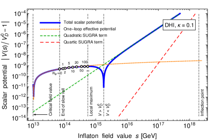
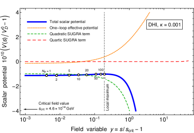
Figure 3: Total scalar potential for the real inflaton field $s$ in D-term hybrid inflation for two representative values of the inflaton Yukawa coupling $\kappa$. Parameter values: (Left panel) $\kappa=10^{-1}$, $\sqrt{\xi}\simeq 6.9\times 10^{15}\,\textrm{GeV}$, $m_{3/2}\simeq 6.9\times 10^{7}\,\textrm{GeV}$ and (Right panel) $\kappa=10^{-3}$, $\sqrt{\xi}\simeq 3.3\times 10^{15}\,\textrm{GeV}$, $m_{3/2}\simeq 1.6\times 10^{7}\,\textrm{GeV}$. In both panels, we set $g=10^{-4}$, which results in a hill top in the potential. Both parameter points are chosen such that they reproduce the measured CMB observables, $A_{s}=A_{s}^{\rm obs}$ and $n_{s}=n_{s}^{\rm obs}$. The potential is always bounded from below and positive at large field values. In both plots, we also compare the quadratic, quartic, and radiative contributions to the total scalar potential.

In the next step, we compute the slow-roll parameters $\varepsilon$ and $\eta$. In parallel to Eq. (49), we obtain

$$\varepsilon=\frac{1}{2}\left(\frac{m_{s}^{2}s^{2}+V_{1\ell}^{0}}{V_{D}^{0}}\right)^{2}\left(\frac{M_{\rm Pl}}{s}\right)^{2}\,,\quad\eta=\Delta-\frac{V_{1\ell}^{0}}{V_{D}^{0}}\left(\frac{M_{\rm Pl}}{s}\right)^{2}\,.$$ (122)

As usual in supersymmetric hybrid inflation, the slow-roll parameter $\varepsilon$ is suppressed by an additional factor $V_{1\ell}^{0}/V_{D}^{0}$ compared to the slow-roll parameter $\eta$. The parameter $\Delta$ in Eq. (122) accounts for the SUGRA correction to $\eta$ in consequence of the tachyonic mass term in Eq. (116) (see also Eq. (57)),

$$\Delta=M_{\rm Pl}^{2}\,\frac{m_{s}^{2}}{V_{D}^{0}}=-\frac{2}{3}\left(\frac{m_{3/2}}{H_{\rm inf}}\right)^{2}\,.$$ (123)

Slow-roll inflation ends and transitions into a fast-roll stage as soon as $\eta$ reaches $\eta_{\rm max}$ (see Eq. (50)),

$$s_{\rm fast}=\left(\frac{V_{1\ell}^{0}}{m_{s}^{2}+m_{\rm max}^{2}}\right)^{1/2}=\frac{g\,M_{\rm Pl}}{\left(4\pi^{2}\,\eta_{\rm max}-2\,g^{2}/\zeta\right)^{1/2}}\,,\quad m_{\rm max}^{2}=\eta_{\rm max}\,\frac{V_{D}^{0}}{M_{\rm Pl}^{2}}\,.$$ (124)

Here, $m_{\rm max}^{2}$ denotes again the maximal curvature of the scalar potential, $V^{\prime\prime}$, that is allowed by the slow-roll bound on the parameter $\eta$. Similarly as in Sec. 3, inflation ends as soon as the inflaton field ceases to slowly roll in the scalar potential (i.e., at $s=s_{\rm fast}$) or once it reaches the critical point in field space that triggers the waterfall transition (i.e., at $s=s_{\rm crit}$), $s_{\rm end}=\max\left\{s_{\rm fast},s_{\rm crit}\right\}$.

In the hill-top regime, the slow-roll equation of motion takes the following form (see also Eq. (56)),

$$\left(s^{2}\right)^{\prime}=2\,\Delta\left(s^{2}-s_{\rm max}^{2}\right)\,,\quad\left(s^{2}\right)^{\prime}=2ss^{\prime}\,,\quad s_{\rm max}^{2}=-\frac{V_{1\ell}^{0}}{m_{s}^{2}}\,.$$ (125)

In combination with the boundary condition $s=s_{\rm end}$ at $N_{e}=0$, this first-order ordinary differential equation has a unique solution that varies exponentially with the number of $e$-folds $N_{e}$,

$$s^{2}\left(N_{e}\right)=s_{\rm max}^{2}\left(1+\overline{W}\right)\,,\quad\overline{W}=\bigg{[}\left(\frac{s_{\rm end}}{s_{\rm max}}\right)^{2}-1\bigg{]}\>e^{2\,\Delta\,N_{e}}\,.$$ (126)

Here, the function $\overline{W}$ plays a role similar to the Lambert W function in Eq. (58). The solution in Eq. (126) can also be written as a function of the three parameters $\eta_{\rm max}$, $N_{e}$, and $\Delta$,

$$s^{2}\left(N_{e}\right)=s_{\rm max}^{2}\left(1+\overline{W}\right)\,,\quad\overline{W}=-\left(1+\frac{\Delta}{\eta_{\rm max}+\Delta}\right)e^{2\,\Delta\,N_{e}}\,.$$ (127)

Together with Eq. (122), this function results in the following compact expressions for $\varepsilon$ and $\eta$,

$$\varepsilon=\left(\frac{s_{\rm max}}{M_{\rm Pl}}\right)^{2}\frac{\left(\overline{W}\Delta\right)^{2}}{2\left(1+\overline{W}\right)}\,,\quad\eta=\frac{\left(2+\overline{W}\right)\Delta}{1+\overline{W}}\,,$$ (128)

from which it is evident that $\varepsilon$ is suppressed w.r.t. $\eta$ by a factor $\Delta\left(s_{\rm max}/M_{\rm Pl}\right)^{2}$. Therefore, to compute the scalar spectral index $n_{s}$, we only need to take into account the slow-roll parameter $\eta$,

$$n_{s}\approx 1+2\,\eta=1+\frac{2\left(2+\overline{W}\right)\Delta}{1+\overline{W}}\,.$$ (129)

For given values of $\eta_{\rm max}$ and $N_{e}$ and requiring that DHI in the large-$\kappa$ regime must result in the correct scalar spectral index, $n_{s}=n_{s}^{\rm obs}$, Eq. (129) can be used to determine the parameter $\Delta$,

$$\eta_{\rm max}=10^{-0.5}\,,\quad N_{*}=47.5\,,\quad n_{s}=n_{s}^{\rm obs}\qquad\Rightarrow\qquad\Delta\simeq-4.9\times 10^{-3}\,.$$ (130)

In contrast to FHI, we now obtain a negative value for $\Delta$. This is a direct consequence of the definition in Eq. (123) and the negative sign of the inflaton mass squared in Eq. (116). Thanks to Eq. (127), the numerical result in Eq. (130) fixes the inflaton field value $s_{*}$ at the time of CMB horizon exit,

$$\eta_{\rm max}=10^{-0.5}\,,\quad N_{*}=47.5\,,\quad\Delta\simeq-4.9\times 10^{-3}\qquad\Rightarrow\qquad\overline{W}\simeq-0.62\,,\quad s_{*}\simeq 0.62\,s_{\rm max}\,.$$ (131)

Accidentally, the ratio $s_{*}/s_{\rm max}$ obtains almost the same value as in the case of FHI (see Eq. (64)). Furthermore, we can use the numerical value for $\Delta$ to fix the relation between $m_{3/2}$ and $H_{\rm inf}$,

$$m_{3/2}=\left(\frac{3}{2}\left|\Delta\right|\right)^{1/2}H_{\rm inf}\simeq 8.6\times 10^{-2}\,H_{\rm inf}\,.$$ (132)

This relation is analogous to Eq. (65). Now, however, we find that the gravitino mass must only be mildly suppressed compared to the Hubble rate. This underlines the importance of the quadratic SUGRA term in the scalar potential — in DHI, the soft inflaton mass term is supposed to result in a relative variation of the slow-roll parameter $\eta$ of $\mathcal{O}\left(1\right)$ in order to achieve the correct value for $n_{s}$. Finally, the numerical $\Delta$ value also provides us with a numerical expression for the parameter $\zeta$,

$$\zeta=\frac{g^{2}}{2\pi^{2}\left|\Delta\right|}\simeq 1.0\times 10^{-7}\>\bigg{(}\frac{g}{10^{-4}}\bigg{)}^{2}\,.$$ (133)

Therefore, for sufficiently small values of $g$, we are always deep inside the hill-top regime. Only for $g\geq\sqrt{2}\,\pi\left|\Delta\right|^{1/2}\simeq 0.31$, we enter the inflection-point regime. However, such large values of $g$ will be less interesting for us, as they turn out to be incompatible with the CDM isocurvature constraint.

Eq. (132) eliminates the gravitino mass as a free parameter from our analysis. Similarly, we can use the observed value of the scalar spectral amplitude, $A_{s}^{\rm obs}$, to eliminate the FI parameter $\xi$. Combining Eqs. (53), (109), (121), (123), and (128), we find the following compact expression,

$$A_{s}=\frac{1+\overline{W}}{6\left|\Delta\right|\overline{W}^{2}}\left(\frac{\sqrt{\xi}}{M_{\rm Pl}}\right)^{4}\,.$$ (134)

The requirement $A_{s}=A_{s}^{\rm obs}$, thus, fixes $\sqrt{\xi}$ to a unique value in direct proximity to the GUT scale,

$$\sqrt{\xi}=\left(6\,A_{s}^{\rm obs}\left|\Delta\right|\frac{\overline{W}^{2}}{1+\overline{W}}\right)^{1/4}M_{\rm Pl}\simeq 6.9\times 10^{15}\,\textrm{GeV}\,.$$ (135)

Remarkably enough, this result is independent of the coupling constants $\kappa$ and $g$. This differs from the situation in FHI, where the F-term mass scale $\mu_{S}$ scales like $\mu_{S}\propto\kappa^{1/2}$ in the large-$\kappa$ regime (see Eq. (68)). Meanwhile, the SSB scale $v$ again obtains a constant value just like in FHI (see Eq. (69)),

$$v=\left(24\,A_{s}^{\rm obs}\left|\Delta\right|\frac{\overline{W}^{2}}{1+\overline{W}}\right)^{1/4}M_{\rm Pl}\simeq 9.8\times 10^{15}\,\textrm{GeV}\,.$$ (136)

DHI saturates the Bogomolny limit (see Eq. (114)). Eq. (136), thus, fixes the cosmic string tension,

$$G\,\mu_{\rm CS}=\left(\frac{3}{8}\,A_{s}^{\rm obs}\left|\Delta\right|\frac{\overline{W}^{2}}{1+\overline{W}}\right)^{1/2}\simeq 2.0\times 10^{-6}\,.$$ (137)

This value violates the upper bound in Eq. (33) by an order of magnitude. For this reason, we are again facing two options. We can either presume that the gauge symmetry $G$ already becomes broken before the end of inflation or have to resort to a different part of parameter space where the cosmic string tension is sufficiently suppressed (see the discussion below Eq. (38)).

An important result of our analysis is that the phenomenology of DHI is obviously insensitive to the precise value of $\kappa$ in the large-$\kappa$ regime. The two conditions $n_{s}=n_{s}^{\rm obs}$ and $A_{s}=A_{s}^{\rm obs}$ therefore reduce the viable parameter space again to a one-dimensional hypersurface. However, this time, this hypersurface is parametrized in terms of the gauge coupling $g$ rather than the Yukawa coupling $\kappa$. Thanks to the numerical result in Eq. (135), we obtain, e.g., for the inflationary Hubble rate

$$H_{\rm inf}=\left|\overline{W}\right|\left(\frac{A_{s}^{\rm obs}\left|\Delta\right|}{1+\overline{W}}\right)^{1/2}g\,M_{\rm Pl}\simeq 8.0\times 10^{8}\,\textrm{GeV}\>\bigg{(}\frac{g}{10^{-4}}\bigg{)}\,.$$ (138)

This expression scales linearly with $g$, which is a completely free parameter for the time being. As a consequence, it is straightforward to reduce the Hubble scale of DHI by lowering $g$. At this point, recall that the beta function of the gauge coupling $g$ is proportional to $g$ itself (at one loop, $\beta_{g}^{1\ell}\propto g^{3}$). Thus, small $g$ values are stable under renormalization group running and, hence, technically natural. The combination of Eqs. (132) and (138) results in the following expression for the gravitino mass,

$$m_{3/2}=\Delta\,\overline{W}\left[\frac{3\,A_{s}^{\rm obs}}{2\left(1+\overline{W}\right)}\right]^{1/2}g\,M_{\rm Pl}\simeq 6.9\times 10^{7}\,\textrm{GeV}\>\bigg{(}\frac{g}{10^{-4}}\bigg{)}\,.$$ (139)

This explicit expression allows us to determine the critical $\kappa$ value $\kappa_{0}$ that separates the large-$\kappa$ regime from the small-$\kappa$ regime. As in the case of FHI, we demand that, for $\kappa\lesssim\kappa_{0},$ the local maximum in the scalar potential is located in the direct vicinity of the critical field value $s_{\rm crit}$,

$$s_{\rm scrit}=s_{\rm max}\qquad\Rightarrow\qquad\kappa_{0}=\frac{4\sqrt{2}\,\pi\,m_{3/2}\left(g\right)}{g\sqrt{\xi}}\simeq 1.8\times 10^{-3}\,.$$ (140)

By accident, this value coincides with the critical $\kappa$ value in FHI (see Eq. (73)).

Eqs. (138) and (139) mark the main technical results in this section. Confronting our result for $H_{\rm inf}$ with the CDM isocurvature constraint in Eq. (15), we obtain the following upper bound on $g$,

$$\boxed{g\lesssim 1.6\times 10^{-4}\left(\frac{1}{F_{\rm DM}^{a}}\right)^{1/2}\left(\frac{f_{a}}{10^{16}\,\textrm{GeV}}\right)^{0.42}}$$ (141)

This bound is independent of the Yukawa coupling $\kappa$ and can, hence, be satisfied for any sensible value of $f_{a}$ without leaving the large-$\kappa$ regime. This is a characteristic advantage of DHI over FHI. Moreover, we find that Planck-scale values of $f_{a}$ result in an upper bound on $g$ of $\mathcal{O}\left(10^{-3}\right)$, which is of the same order of magnitude as the upper bound on $\kappa$ in Eq. (74). This statement remains unaffected if one also accounts for the upper bound on $f_{a}$ from black hole superradiance. Together with Eq. (139), the upper bound in Eq. (141) can be used to obtain an upper bound on $m_{3/2}$,

$$\boxed{m_{3/2}\lesssim 1.1\times 10^{8}\,\textrm{GeV}\left(\frac{1}{F_{\rm DM}^{a}}\right)^{1/2}\left(\frac{f_{a}}{10^{16}\,\textrm{GeV}}\right)^{0.42}}$$ (142)

which is weaker than the corresponding bound in Eq. (75) by several orders of magnitude. This is easily explained by the fact that, unlike FHI, DHI requires a large $m_{3/2}$–$H_{\rm inf}$ ratio in order to reproduce the observed value of the scalar spectral index (see the discussion below Eq. (132)). In Fig. 4, we illustrate the implications of the CDM isocurvature constraint for the parameter space of DHI. The plots in this figure are based on a fully numerical analysis of slow-roll inflation in the complete scalar potential of DHI (see Eqs. (106), (109), and (113)). Again, we find excellent agreement between the numerical data and the analytical results derived in this section.

Finally, we use the expressions in Eqs. (138) and (139) to identify the region in parameter space where the PQ symmetry remains unbroken during inflation. In analogy to Eq. (76), we find

$$g\gtrsim 1.3\times 10^{-3}\left(\frac{f_{a}}{10^{10}\,\textrm{GeV}}\right)\,,\quad m_{3/2}\gtrsim 8.6\times 10^{8}\,\textrm{GeV}\left(\frac{f_{a}}{10^{10}\,\textrm{GeV}}\right)\,.$$ (143)

For small $f_{a}$ and large values of $g$ and $m_{3/2}$, one might therefore encounter a domain wall problem.

4.3 Inflation close to the waterfall phase transition

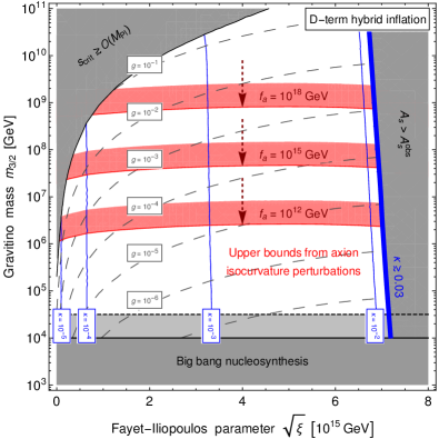
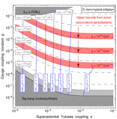
Figure 4: Parameter values for D-term hybrid inflation that reproduce the CMB data, $A_{s}=A_{s}^{\rm obs}$ and $n_{s}=n_{s}^{\rm obs}$, in combination with the CDM isocurvature constraint for several values of the axion decay constant and different assumptions regarding the axion DM fraction. The stronger [weaker] bounds correspond to $F_{\rm DM}^{a}=1$ [$F_{\rm DM}^{a}=0.1$]. (Left panel) Two-dimensional region in the $\sqrt{\xi}$–$m_{3/2}$ plane that manages to reproduce the observed CMB data. (Right panel) FI scale $\sqrt{\xi}$ and gravitino mass $m_{3/2}$ as functions of the Yukawa coupling $\kappa$ and the gauge coupling $g$. Both plots are based on a numerical analysis that accounts for the complete scalar potential in Eqs. (106) and (113).

In the case of FHI, the CDM isocurvature constraint forces one to venture into the small-$\kappa$ regime for all but the largest $f_{a}$ values. As we saw in the previous section, this is no longer necessary in DHI, where small $g$ values allow one to avoid large axion isocurvature perturbations even in the large-$\kappa$ regime. Nonetheless, we shall also study the dynamics of DHI for small $\kappa$ values. On the one hand, this will serve the purpose of completing our systematic study of supersymmetric hybrid inflation for large and small Yukawa couplings. On the other hand, small $\kappa$ values will again turn out to be the means of choice to suppress the cosmic string tension. At the same time, the small-$\kappa$ regime of DHI faces the same challenges w.r.t. the initial conditions of inflation as the small-$\kappa$ regime of FHI (see the first paragraph of Sec. 3.3 and the right panel of Fig. 3). This means that a suppressed cosmic string tension can again only be achieved at the cost of a somewhat tuned initial field value.

To obtain the scalar potential in the small-$\kappa$ regime, we are able to proceed in the same way as in Sec. 3.3. That is, we have to replace the logarithm $\ln\left(x\right)$ in Eq. (116) by the function $L_{2}\left(y\right)$,

$$V\simeq V_{D}^{0}+\frac{1}{2}\,m_{s}^{2}\,s^{2}+\frac{1}{2}\,V_{1\ell}^{0}\,L_{2}\left(y\right)\,,$$ (144)

where we again neglected the quartic SUGRA term. Correspondingly, $\varepsilon$ and $\eta$ in Eq. (122) turn into

$$\varepsilon=\frac{1}{2}\left(\frac{m_{s}^{2}s_{\rm crit}s+c_{1}V_{1\ell}^{0}/2}{V_{D}^{0}}\right)^{2}\left(\frac{M_{\rm Pl}}{s_{\rm crit}}\right)^{2}\,,\quad\eta=\Delta+\frac{V_{1\ell}^{0}}{2\,V_{D}^{0}}\left(c_{2}+\frac{3}{2}\,\bar{c}_{2}+\bar{c}_{2}\ln y\right)\left(\frac{M_{\rm Pl}}{s_{\rm crit}}\right)^{2}\,.$$ (145)

In contrast to FHI in the small-$\kappa$ regime, the parameter $\varepsilon$ now receives a field-dependent contribution from the quadratic mass term in Eq. (144). This contribution comes with a negative sign (recall that $m_{s}^{2}<0$), which is responsible for the presence of the local maximum at $s_{\rm max}$. In the small-$\kappa$ regime, the field value $s_{\rm max}$ follows from the requirement that $\varepsilon$ in Eq. (145) must vanish at $s=s_{\rm max}$,

$$s_{\rm max}=-\frac{c_{1}V_{1\ell}^{0}}{2\,s_{\rm crit}\,m_{s}^{2}}=\frac{\ln 2\,g^{3}\kappa}{8\sqrt{2}\,\pi^{2}}\left(\frac{\sqrt{\xi}}{m_{3/2}}\right)^{2}\sqrt{\xi}\,.$$ (146)

This expression comes in handy when writing down the slow-roll equation of motion for the inflaton,

$$s^{\prime}=\Delta\left(s-s_{\rm max}\right)\,,$$ (147)

where $\Delta$ is still defined as in Eq. (123). Together with the boundary condition $s=s_{\rm crit}$ at $N_{e}=0$, the differential equation in Eq. (147) has a unique solution in terms of a simple exponential function,

$$s\left(N_{e}\right)=s_{\rm max}+\left(s_{\rm crit}-s_{\rm max}\right)e^{\Delta\,N_{e}}\,.$$ (148)

This result allows us to write down explicit expressions for $\varepsilon$ and $\eta$ as functions of $y_{\rm max}$, $N_{e}$, and $\Delta$,

$$\varepsilon =\bigg{(}\frac{g}{4\pi}\bigg{)}^{2}\left(\frac{y_{\rm max}}{1+y_{\rm max}}\right)^{2}c_{1}\,e^{2\,\Delta\,N_{e}}\left|\Delta\right|\,,$$ (149)

$$\eta =\Delta-\Delta\left(y_{\rm max}+1\right)\left[\frac{c_{2}}{c_{1}}+\frac{3\,\bar{c}_{2}}{2\,c_{1}}+\frac{\bar{c}_{2}}{c_{1}}\ln\left(y_{\rm max}\left(1-e^{\Delta\,N_{e}}\right)\right)\right]\,,$$

where $y_{\rm max}=s_{\rm max}/s_{\rm crit}-1$ (see also Eq. (77)). Again, we notice that $\varepsilon$ is suppressed w.r.t. $\eta$.

Next, we use the two conditions $A_{s}=A_{s}^{\rm obs}$ and $n_{s}=n_{s}^{\rm ons}$ to determine the two parameters $y_{\rm max}$ and $\Delta$. First, let us consider the amplitude of the scalar power spectrum. Combining our results in Eqs. (53), (109), (123), (146), and (149), a straightforward calculation provides us with

$$A_{s}=\frac{c_{1}}{3}\left(\frac{\kappa}{4\pi}\right)^{4}\frac{e^{-2\,\Delta\,N_{e}}}{\left(y_{\rm max}+1\right)y_{\rm max}^{2}\left|\Delta\right|^{3}}\approx\frac{c_{1}}{3}\left(\frac{\kappa}{4\pi}\right)^{4}\frac{e^{-2\,\Delta\,N_{e}}}{y_{\rm max}^{2}\left|\Delta\right|^{3}}\,.$$ (150)

Here, we made use of the fact that $y_{\rm max}$ is much smaller than unity in the small-$\kappa$ regime, $y_{\rm max}\ll 1$. Imposing the condition that $A_{s}$ must reproduce $A_{s}^{\rm obs}$, we are able to solve Eq. (150) for $y_{\rm max}$,

$$y_{\rm max}=\left(\frac{c_{1}}{3A_{s}^{\rm obs}}\right)^{1/2}\bigg{(}\frac{\kappa}{4\pi}\bigg{)}^{2}\>\frac{e^{-\Delta\,N_{e}}}{\left|\Delta\right|^{3/2}}\,,$$ (151)

which is suppressed by two powers of the small factor $\kappa/\left(4\pi\right)$. Together with Eq. (149), this result allows us to write down the scalar spectral index $n_{s}$ as a function of $N_{e}$, $\Delta$, and $\kappa$. As before, we will neglect the slow-roll parameter $\varepsilon$ and simply approximate $n_{s}$ by $n_{s}\approx 1+2\,\eta$. We, thus, obtain

$$n_{s}\approx 1+2\,\Delta-2\,\Delta\left[\frac{c_{2}}{c_{1}}+\frac{3\,\bar{c}_{2}}{2\,c_{1}}+\frac{\bar{c}_{2}}{c_{1}}\ln\bigg{(}\left(\frac{c_{1}}{3A_{s}^{\rm obs}}\right)^{1/2}\bigg{(}\frac{\kappa}{4\pi}\bigg{)}^{2}\>\frac{e^{-\Delta\,N_{e}}-1}{\left|\Delta\right|^{3/2}}\bigg{)}\right]\,.$$ (152)

For a fixed value of $N_{e}$, the condition $n_{s}=n_{s}^{\rm obs}$ can be numerically solved for $\Delta$ as a function of $\kappa$,

$$\quad N_{e}=47.5\,,\quad n_{s}=n_{s}^{\rm obs}\qquad\Rightarrow\qquad\Delta\simeq-1.2\times 10^{-3}\>\bigg{(}\frac{\kappa}{10^{-5}}\bigg{)}^{p}\,,\quad p=0.14\,.$$ (153)

Evidently, $\Delta$ depends only very weakly on the Yukawa coupling $\kappa$. The slight numerical uncertainty in the exponent $p$ is therefore irrelevant for all practical purposes. In fact, we checked that the power law in Eq. (153) represents an adequate fit to the exact numerical result for all relevant $\kappa$ values deep inside the small-$\kappa$ regime, $\kappa\lesssim\mathcal{O}\left(10^{-4}\right)$. Together with Eq. (151), we now obtain for $y_{\rm max}$,

$$y_{\rm max}\simeq 3.1\times 10^{-4}\>\bigg{(}\frac{\kappa}{10^{-5}}\bigg{)}^{1.79}\,,$$ (154)

which is, indeed, much smaller than unity as long as $\kappa$ is sufficiently small.

With the numerical expressions in Eqs. (153) and (154) at our disposal, we are now ready to compute the mass scales that are relevant in the description of DHI for small $\kappa$ values. As in Sec. 4.2, we first consider the FI mass scale $\sqrt{\xi}$. Making use of Eqs. (123) and (146), we find

$$\sqrt{\xi}=\left(\frac{c_{1}}{\left(1+y_{\rm max}\right)\left|\Delta\right|}\right)^{1/2}\frac{\kappa}{4\pi}\,M_{\rm Pl}\simeq 9.2\times 10^{13}\,\textrm{GeV}\>\bigg{(}\frac{\kappa}{10^{-5}}\bigg{)}^{0.93}\,.$$ (155)

In contrast to the value in Eq. (135), this result is suppressed by the small Yukawa coupling $\kappa$ and, hence, parametrically smaller than $\Lambda_{\rm GUT}$. The same applies to the value of the SSB scale $v$,

$$v=\left(\frac{2\,c_{1}}{\left(1+y_{\rm max}\right)\left|\Delta\right|}\right)^{1/2}\frac{\kappa}{4\pi}\,M_{\rm Pl}\simeq 1.3\times 10^{14}\,\textrm{GeV}\>\bigg{(}\frac{\kappa}{10^{-5}}\bigg{)}^{0.93}\,.$$ (156)

As a consequence, the cosmic string tension turns out to be suppressed by almost two powers of $\kappa$,

$$G\,\mu_{\rm CS}=\frac{c_{1}}{4\left(1+y_{\rm max}\right)\left|\Delta\right|}\>\bigg{(}\frac{\kappa}{4\pi}\bigg{)}^{2}\simeq 3.5\times 10^{-10}\>\bigg{(}\frac{\kappa}{10^{-5}}\bigg{)}^{1.86}\,.$$ (157)

Similarly as in FHI, it is therefore always possible to avoid the cosmic string bound in Eq. (33) by choosing $\kappa$ small enough. This resolves the cosmic string problem of DHI at the price of fine-tuned initial conditions. We also note that the mass scales $\sqrt{\xi}$ and $v$ are solely controlled by $\kappa$. This is no longer the case for the Hubble rate $H_{\rm inf}$, which depends on both $\kappa$ and $g$ (see Eq. (110)),

$$H_{\rm inf}=\frac{c_{1}\,g}{\sqrt{6}\left(1+y_{\rm max}\right)\left|\Delta\right|}\>\bigg{(}\frac{\kappa}{4\pi}\bigg{)}^{2}M_{\rm Pl}\simeq 1.4\times 10^{7}\,\textrm{GeV}\>\bigg{(}\frac{g}{10^{-2}}\bigg{)}\bigg{(}\frac{\kappa}{10^{-5}}\bigg{)}^{1.86}\,.$$ (158)

This result illustrates that, at small $\kappa$ values, the Hubble rate approximately scales like $H_{\rm inf}\propto g\kappa^{2}$. It is, thus, possible to suppress $H_{\rm inf}$ by a small $\kappa$ value while keeping $g$ moderately large. This is an important difference from the large-$\kappa$ regime where $H_{\rm inf}$ can only be suppressed by small values of $g$ (see Eq. (138)). The situation is similar for the gravitino mass for which we obtain (see Eq. (132))

$$m_{3/2}=\frac{c_{1}\,g}{2\left(1+y_{\rm max}\right)\left|\Delta\right|^{1/2}}\>\bigg{(}\frac{\kappa}{4\pi}\bigg{)}^{2}M_{\rm Pl}\simeq 6.1\times 10^{5}\,\textrm{GeV}\>\bigg{(}\frac{g}{10^{-2}}\bigg{)}\bigg{(}\frac{\kappa}{10^{-5}}\bigg{)}^{1.93}\,.$$ (159)

For the fourth and last time, we are now able to use our results and constrain the viable parameter space by means of the CDM isocurvature constraint in Eq. (15). Together, Eqs. (15) and (158) yield

$$\boxed{g\lesssim 2.0\times 10^{-2}\left(\frac{10^{-5}}{\kappa}\right)^{1.86}\left(\frac{1}{F_{\rm DM}^{a}}\right)^{1/2}\left(\frac{f_{a}}{10^{12}\,\textrm{GeV}}\right)^{0.42}}$$ (160)

This bound is weaker than the one in Eq. (141), which reflects the fact that, now, the Hubble rate $H_{\rm inf}$ is suppressed by the small values of both $\kappa$ and $g$. In particular, we note that $g$ can now even be larger than $\mathcal{O}\left(10^{-3}\right)$. However, it is important to remember that this is only possible as long as we are in the small-$\kappa$ regime, i.e., as long as $\kappa\lesssim\mathcal{O}\left(10^{-3}\right)$ (see Eq. (140)). In summary, we therefore conclude that, also in the small-$\kappa$ regime, at least one coupling constant must not be larger than $\mathcal{O}\left(10^{-3}\right)$. This completes our analysis of the upper bounds on $\kappa$ and $g$ in consequence of the CDM isocurvature constraint. Our main result according to Eqs. (74), (97), (141), and (160) is that

Supersymmetric hybrid inflation complies with the CDM isocurvature constraint if an appropriate (Yukawa or gauge) coupling constant is set to a value of $\mathit{\mathcal{O}\left(10^{-3}\right)}$ or smaller.

The upper bound in Eq. (160) can also be used to derive an upper bound on $m_{3/2}$ (see Eq. (159)),

$$\boxed{m_{3/2}\lesssim 1.2\times 10^{6}\,\textrm{GeV}\>\bigg{(}\frac{\kappa}{10^{-5}}\bigg{)}^{0.07}\left(\frac{1}{F_{\rm DM}^{a}}\right)^{1/2}\left(\frac{f_{a}}{10^{12}\,\textrm{GeV}}\right)^{0.42}}$$ (161)

This bound is stronger than the one in Eq. (142), which is consistent with the fact that, in the small-$\kappa$ regime, all mass scales are subject to an additional suppression by the small value of $\kappa$. Eq. (161) completes our analysis of the upper bounds on $m_{3/2}$. Similarly as for $\kappa$ and $g$, we are now able to compare and summarize the bounds in Eq. (75), (98), (142), and (161). We conclude that

For $\mathit{f_{a}}$ as large as $\mathit{f_{a}\sim M_{\textrm{{Pl}}}}$, the CDM isocurvature constraint translates into absolute upper bounds on the gravitino mass of $\mathit{\mathcal{O}\left(10^{5}\right)\,\textrm{{GeV}}}$ in FHI and $\mathit{\mathcal{O}\left(10^{9}\right)\,\textrm{{GeV}}}$ in DHI.

The analytical results in Eqs. (160) and (161) need to be compared with the fully numerical result in Fig. 4. Once again, we find excellent agreement. Furthermore, we can use our result for $G\,\mu_{\rm CS}$ in Eq. (157) to determine the range of $\kappa$ values that allow to satisfy the upper bound on the cosmic string tension. Together with Eq. (161), we find the following upper bounds on $\kappa$ and $m_{3/2}$,

$$G\,\mu_{\rm CS}<G\,\mu_{\rm CS}^{\rm max}\qquad\Rightarrow\qquad\kappa\lesssim 2.1\times 10^{-4}\,,\quad m_{3/2}\lesssim 2.1\times 10^{8}\,\textrm{GeV}\>\bigg{(}\frac{g}{10^{-2}}\bigg{)}\,.$$ (162)

The upper bound on $\kappa$ is slightly smaller than the critical $\kappa$ value in Eq. (140). This means that the cosmic string bound can only be circumvented for $\kappa$ values deep inside the small-$\kappa$ regime. For all other $\kappa$ values, we have to assume that no cosmic strings are produced at the end of inflation. Making use of Eqs. (155), (156), and (158), the constraints in Eq. (162) can also be translated into

$$v\lesssim 2.2\times 10^{15}\,\textrm{GeV}\,,\quad\sqrt{\xi}\lesssim 1.5\times 10^{15}\,\textrm{GeV}\,,\quad H_{\rm inf}\lesssim 4.0\times 10^{9}\,\textrm{GeV}\>\bigg{(}\frac{g}{10^{-2}}\bigg{)}\,.$$ (163)

The result is consistent with the bound on the FI mass scale $\sqrt{\xi}$ in Eq. (115).

Finally, we use the expressions in Eqs. (158) and (159) to identify the region in parameter space where the PQ symmetry remains unbroken during inflation. In analogy to Eq. (101), we find

$$g\gtrsim 7.1\times 10^{-2}\left(\frac{10^{-5}}{\kappa}\right)^{1.86}\left(\frac{f_{a}}{10^{8}\,\textrm{GeV}}\right)\,,\quad m_{3/2}\gtrsim 4.3\times 10^{6}\,\textrm{GeV}\>\bigg{(}\frac{\kappa}{10^{-5}}\bigg{)}^{0.07}\left(\frac{f_{a}}{10^{8}\,\textrm{GeV}}\right)\,.$$ (164)

However, this time, we must be careful when asking for the interpretation of these results. For values of $g$ and $m_{3/2}$ as large as those in Eq. (164), the critical field value $s_{\rm crit}$ begins to exceed the Planck scale (see Eq. (112)). Thus, in this part of parameter space, inflaton occurs at super-Planckian field values where we have less control over the SUGRA corrections to the scalar potential. In this paper, we decided to restrict ourselves to regions in parameter space where $s_{\rm crit}\lesssim\mathcal{O}\left(M_{\rm Pl}\right)$. For this reason, the bounds in Eq. (164) are irrelevant for our purposes as soon as they are in conflict with Eq. (112).

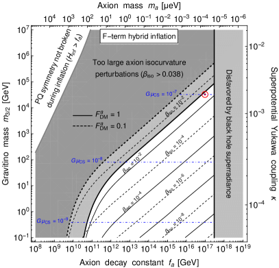
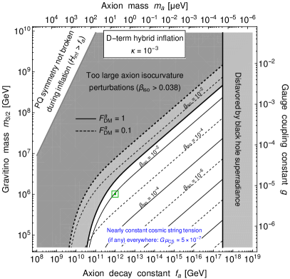
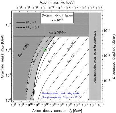
Figure 5: Bounds on the parameter space of (upper left panel) F-term hybrid inflation for all possible $\kappa$ values, (upper right panel) D-term hybrid inflation for $\kappa=10^{-1}$, (lower left panel) D-term hybrid inflation for $\kappa=10^{-3}$, (lower right panel) D-term hybrid inflation for $\kappa=10^{-5}$. All plots are based on a fully numerical analysis. The analytical expressions for the upper bounds on the gravitino mass can be found in Eqs. (75), (98), (142), and (161). The lower bounds that lead to the postinflationary PQSB scenario can be found in Eqs. (76), (101), (143), and (164). Analytical expressions for the cosmic string tension are contained in Eqs. (70), (93), (137), and (157). The constraints on the axion decay constant from black hole superradiance, $3\times 10^{17}\lesssim f_{a}/\textrm{GeV}\lesssim 10^{19}$, are taken from [123, 125, 126]. The red circle (in the upper left panel, at $f_{a}=10^{17}\,\textrm{GeV}$ and $m_{3/2}=30\,\textrm{TeV}$) as well as the green square (in all other panels, at $f_{a}=10^{12}\,\textrm{GeV}$ and $m_{3/2}=1000\,\textrm{TeV}$) denote the two benchmark points discussed in Sec. 5.

5 Benchmark scenarios

In the two previous sections, we presented a detailed slow-roll analysis that enabled us to assess the consequences of the CDM isocurvature constraint in Eq. (15) for supersymmetric hybrid inflation. Our main results are summarized in Fig. 5. The four plots in this figure show the various upper and lower bounds that we obtained throughout our analysis in dependence of the axion decay constant $f_{a}$. For both FHI and DHI, we conclude that it turns out to be quite easy to satisfy the requirement of small axion isocurvature perturbations. In fact, for both types of supersymmetric hybrid inflation, we find large regions in parameter space that are consistent with all observational constraints, including the measured values of the inflationary CMB observables $A_{s}$ and $n_{s}$ as well as the upper bound on the cosmic string tension $G\,\mu_{\rm CS}$. To explore the physical implications of our results a bit further, let us now elaborate on two characteristic benchmark scenarios in the viable part of parameter space (see the red circle in the upper left panel of Fig. 5 as well as the green square in all other panels of Fig. 5). This discussion will help us illustrate in an exemplary fashion the possible conclusions that one can draw from our numerical results in Fig. 5. For both benchmark points, we list the defining parameter values as well as the corresponding predictions for all dependent quantities in Tab. 1.

Benchmark point I

First, let us consider FHI for $m_{3/2}=30\,\textrm{TeV}$, $f_{a}=10^{17}\,\textrm{GeV}$, and $F_{\rm DM}^{a}=1$. Here, the large gravitino mass is characteristic for models of high-scale supersymmetry that mostly rely on gravitational effects to mediate the spontaneous breaking of supersymmetry to the visible sector [143, 144, 145]. A minimal example for such a scenario is, e.g., the mediation scheme of pure gravity mediation [146, 147, 148] (see also [149]). The large value of the axion decay constant is inspired by string theory, which typically predicts $f_{a}$ values of the order of $f_{a}\sim 10^{16}\cdots 10^{17}\,\textrm{GeV}$ [122, 123, 124]. For $f_{a}=10^{17}\,\textrm{GeV}$, the axion is expected to have a tiny mass, $m_{a}\simeq 5.7\times 10^{-5}\,\textrm{\lx@text@micro\hskip 0.5pteV}$ (see Eq. (2)). Remarkably enough, this falls into the range of masses that might be probed by CASPEr [150], a proposed magnetometry experiment that aims at measuring the precession of nuclear spins induced by their interaction with the axion DM background. At the same time, an axion decay constant as large as $f_{a}=10^{17}\,\textrm{GeV}$ implies that the initial misalignment angle $\bar{\theta}_{\rm ini}$ must be fine-tuned to a relatively small value, $\bar{\theta}_{\rm ini}/\pi\simeq 3.5\times 10^{-4}$, in order to avoid the overproduction of DM (see Eq. (6)). Such a small value may, e.g., be the outcome of anthropic selection in a landscape of string vacua. But irrespective of that, one should also keep in mind that tuning $\bar{\theta}_{\rm ini}$ at the level of $1$ in $10^{3}$ is certainly less severe than tuning the bare vacuum angle $\bar{\theta}$ to a value less than $10^{-10}$ by brute force.

The two observational constraints $A_{s}=A_{s}^{\rm obs}$ and $n_{s}=n_{s}^{\rm obs}$ effectively reduce the viable parameter space of FHI to a one-dimensional hypersurface (see Fig. 2). Our choice of $m_{3/2}$ therefore fixes all other model parameters of FHI. For $m_{3/2}=30\,\textrm{TeV}$, consistency with the scalar CMB power spectrum requires an inflaton Yukawa coupling $\kappa\simeq 1.7\times 10^{-3}$ and an inflaton F-term mass scale $\mu_{S}\simeq 1.1\times 10^{14}\,\textrm{GeV}$. In view of the critical $\kappa$ value in Eq. (73), $\kappa_{0}\simeq 1.8\times 10^{-3}$, this indicates that benchmark point I is located just in the transition region in between the large-$\kappa$ regime and the small-$\kappa$ regime. As a consequence, the initial inflaton field value needs to be slightly tuned, so as to make sure that the inflaton rolls into the correct direction in field space (see the right panel of Fig. 1). However, compared to the situation deep inside the small-$\kappa$ regime, this tuning is still comparatively mild. The required values of $\kappa$ and $\mu_{S}$, moreover, imply a SSB scale during the waterfall transition of $v\simeq 3.6\times 10^{15}\,\textrm{GeV}$. This value lies within an order of magnitude of the GUT scale, $\Lambda_{\rm GUT}\sim 10^{16}\,\textrm{GeV}$, which might hint at a possible connection between FHI and grand unification.

The required F-term mass scale $\mu_{S}$ also determines the Hubble rate during inflation, $H_{\rm inf}\simeq 2.6\times 10^{9}\,\textrm{GeV}$. Given the large value of the axion decay constant, this result complies with the CDM isocurvature constraint in Eq. (15). In fact, for $H_{\rm inf}\simeq 2.6\times 10^{9}\,\textrm{GeV}$, $f_{a}=10^{17}\,\textrm{GeV}$, and $F_{\rm DM}^{a}=1$, we expect a primordial isocurvature fraction $\beta_{\rm iso}\simeq 2.5\times 10^{-2}$, which is smaller than the current upper bound on $\beta_{\rm iso}$ by roughly $30\,\%$. The observational sensitivity to $\beta_{\rm iso}$ is limited by cosmic variance and predicted to be around $\beta_{\rm iso}\simeq 10^{-2}$ (see, e.g., [46]). An ultimate CMB experiment limited only by cosmic variance may therefore be able to detect the primordial axion isocurvature perturbations that contribute to the scalar CMB power spectrum in this benchmark scenario. These are exciting prospects that illustrate how future axion and CMB experiments will help shed more light on the possible interplay of supersymmetry breaking, inflation, and axion physics.

Finally, we comment on the issue of cosmic strings in benchmark scenario I. For $\kappa=1.7\times 10^{-3}$, we predict a cosmic string tension $G\,\mu_{\rm CS}\simeq 9.7\times 10^{-8}$, which just falls short of the current upper bound in Eq. (33). Therefore, if cosmic strings should, indeed, be produced during the waterfall transition at the end of inflation, any improvement over the current bound in the near future should provide clues for the presence of cosmic strings. On the other hand, we caution that a nondetection of cosmic strings would not immediately rule out benchmark point I. In this case, the local gauge symmetry in the waterfall sector may simply be broken in a different sector already before the end of inflation (see the discussion below Eq. (38)). The same conclusion applies if one contrasts our prediction $G\,\mu_{\rm CS}\simeq 9.7\times 10^{-8}$ with less conservative bounds on $G\,\mu_{\rm CS}$ (see, e.g., [110, 111, 112, 113]).

		Benchmark point I	Benchmark point II
Inflation model		FHI	DHI
Gravitino mass $m_{3/2}$	[TeV]	$30$	$1000$
Axion decay constant $f_{a}$	[GeV]	$10^{17}$	$10^{12}$
Axion DM fraction $F_{\rm DM}^{a}$	[%]	$100$	$100$
Axion mass $m_{a}$	[µ eV]	$5.7\times 10^{-5}$	$5.7$
Misalignment angle $\bar{\theta}_{\rm ini}$	[$\pi$]	$3.5\times 10^{-4}$	$0.28$
Yukawa coupling $\kappa$		$1.7\times 10^{-3}$	$10^{-5}$	$10^{-3}$	$10^{-1}$
Gauge coupling $g$		$0.72$	$1.7\times 10^{-2}$	$6.1\times 10^{-6}$	$1.4\times 10^{-6}$
SSB scale $v$	[GeV]	$3.6\times 10^{15}$	$1.3\times 10^{14}$	$4.7\times 10^{15}$	$1.0\times 10^{16}$
F-term mass scale $\mu_{S}$	[GeV]	$1.1\times 10^{14}$	——	——	——
FI mass scale $\sqrt{\xi}$	[GeV]	——	$9.1\times 10^{13}$	$3.3\times 10^{15}$	$7.0\times 10^{15}$
Hubble rate $H_{\rm inf}$	[GeV]	$2.6\times 10^{9}$	$2.3\times 10^{7}$	$1.1\times 10^{7}$	$1.2\times 10^{7}$
CS tension $G\,\mu_{\rm CS}$ (if any)		$9.7\times 10^{-8}$	$3.5\times 10^{-10}$	$4.6\times 10^{-7}$	$2.1\times 10^{-6}$
Isocurvature fraction $\beta_{\rm iso}$		$2.5\times 10^{-2}$	$3.5\times 10^{-2}$	$8.4\times 10^{-3}$	$9.6\times 10^{-3}$

Table 1: Parameter values and predictions for several observables for the two benchmark points discussed in Sec. 5. Benchmark point I is based on F-term hybrid inflation and assumes that the QCD axion has its dynamical origin in string theory (viz., $f_{a}=10^{17}\,\textrm{GeV}$). Benchmark point II is, by contrast, based on D-term hybrid inflation and assumes that the QCD axion has its dynamical origin in field theory (viz., $f_{a}=10^{12}\,\textrm{GeV}$). Both points are also shown in Fig. 5 (see the red circle in the upper left panel of Fig. 5 as well as the green square in all other panels of Fig. 5).

Benchmark point II

Next, we consider DHI for $m_{3/2}=1000\,\textrm{TeV}$, $f_{a}=10^{12}\,\textrm{GeV}$, and $F_{\rm DM}^{a}=1$. Again, the large value of the gravitino mass is inspired by high-scale SUSY scenarios such as pure gravity mediation. Now, however, we choose $m_{3/2}$ towards the upper end of the expected range of values. Such a large gravitino mass may be instrumental in suppressing the rate of dangerous flavor-changing neutral currents [151]. Meanwhile, the chosen value of the axion decay constant corresponds to the upper end of the classical axion window that allows to generate axion DM without any fine-tuning in the initial misalignment angle (see Eq. (4)). Indeed, for $f_{a}=10^{12}\,\textrm{GeV}$, we require an initial misalignment angle $\bar{\theta}_{\rm ini}/\pi\simeq 0.28$ to achieve pure axion DM (i.e., $F_{\rm DM}^{a}=1$), which is a natural value. At the same time, an axion decay constant $f_{a}=10^{12}\,\textrm{GeV}$ is a typical value that can be easily realized in field-theoretic implementations of the Peccei-Quinn mechanism (see, e.g., [152, 153]). An important consequence of the lower axion decay constant compared to benchmark scenario I is a correspondingly heavier axion, $m_{a}\simeq 5.7\,\textrm{\lx@text@micro\hskip 0.5pteV}$ (see Eq. (2)). Axion DM in this mass range will be probed by ADMX [154] and CULTASK [155], two microwave cavity experiments that aim at detecting the resonant conversion of axions into photons in a strong magnetic field.

To make use of the observational constraints $A_{s}=A_{s}^{\rm obs}$ and $n_{s}=n_{s}^{\rm obs}$, we need to fix one more model parameter. For definiteness, we will take this parameter to be the Yukawa coupling $\kappa$ and compare the predictions of DHI for three different $\kappa$ values in the following, $\kappa=10^{-5}$, $10^{-3}$, $10^{-1}$ (see the upper right and the two lower panels of Fig. 5). These values are chosen such that they give a characteristic impression of the viable parameter space for small ($\kappa=10^{-5}$), intermediate ($\kappa=10^{-3}$), and large $\kappa$ values ($\kappa=10^{-1}$). Together with our choice of $m_{3/2}$, the three benchmark values for $\kappa$ allow us to determine the gauge coupling constant $g$, the SSB scale $v$, the FI mass scale $\sqrt{\xi}$, and the Hubble rate $H_{\rm inf}$ (see Fig. 4 and Tab. 1). From the numerical results in Tab. 1, it is evident that, among the three $\kappa$ values under consideration, $\kappa=10^{-1}$ is arguably the most attractive one. Not only does it require the least tuning of the initial inflaton field value (see Fig. 3), but it also results in a SSB scale of exactly $v=1.0\times 10^{16}\,\textrm{GeV}$. Benchmark point II in combination with $\kappa=10^{-1}$ therefore suggests a possible connection between DHI and grand unification.

The three different values of the Hubble rate in Tab. 1 are all of the same order of magnitude, $H_{\rm inf}\sim 10^{7}\,\textrm{GeV}$. By construction, these values are small enough to comply with the CDM isocurvature constraint in Eq. (15). Recall that, depending on the precise value of $\kappa$, a suppressed Hubble rate can be either achieved by a small gauge coupling $g$ (see Eq. (138)) or by a small Yukawa coupling $\kappa$ (see Eq. (158)). This is also reflected in the different $\kappa$ and $g$ values in Tab. 1. In combination with $f_{a}=10^{12}\,\textrm{GeV}$ and $F_{\rm DM}^{a}=1$, the $H_{\rm inf}$ values in Tab. 1 allow us to compute the primordial isocurvature fraction $\beta_{\rm iso}$. For $\kappa=10^{-3}$ and $\kappa=10^{-1}$, we find $\beta_{\rm iso}\sim 10^{-2}$, which may or may not be within reach of an ultimate CMB experiment. For $\kappa=10^{-5}$, on the other hand, we obtain $\beta_{\rm iso}\simeq 3.5\times 10^{-2}$, which is only roughly $8\,\%$ smaller than the current upper bound. Here, the fact that we find different predictions for $\beta_{\rm iso}$ in dependence of $\kappa$ is a consequence of the slightly different $\kappa$ dependence of $H_{\rm inf}$ and $m_{3/2}$ in Eqs. (158) and (159). From this perspective, smaller $\kappa$ values appear more favorable, as they push $\beta_{\rm iso}$ further into the observable range. Similarly, smaller Yukawa couplings also help suppress the cosmic string tension (see Tab. 1). Indeed, only for $\kappa=10^{-5}$, we find a cosmic string tension in accord with the upper bound in Eq. (33). For $\kappa=10^{-3}$ and $\kappa=10^{-1}$, we have to assume again that no cosmic strings are produced during the waterfall transition.

6 Conclusions

The PQ mechanism constitutes a well-motivated BSM scenario that offers not only an attractive solution to the strong $CP$ problem but also a viable particle candidate for DM — the QCD axion. A consistent implementation of the PQ mechanism into inflationary cosmology can, however, be challenging, depending on the details of the underlying model of PQ symmetry breaking. That is, if the global PQ symmetry is spontaneously broken only after inflation, one encounters a domain wall problem, unless domain walls decay sufficiently fast for one reason or another. On the other hand, if the global PQ symmetry is already broken during inflation and not restored afterwards, quantum fluctuations of the axion field during inflation can result in primordial CDM isocurvature perturbations that exceed the current upper bound on the primordial isocurvature fraction $\beta_{\rm iso}$.

The main purpose of this paper was to demonstrate that the axion isocurvature perturbations problem in the preinflationary PQSB scenario can be easily solved in the context of supersymmetric hybrid inflation. To this end, we studied in detail the slow-roll dynamics of both FHI and DHI. These models represent interesting inflationary scenarios that feature a rapid second-order phase transition at the end of inflation, which can be identified with the spontaneous breaking of a local GUT symmetry. For both FHI and DHI, we explicitly accounted for the effect of spontaneous SUSY breaking in a hidden Polonyi sector, which gave us additional control over the shape of the scalar potential. In FHI, the leading soft contribution to the scalar potential turns out to be a linear tadpole term, while in DHI, one obtains a quadratic mass term. The sizes of both terms are controlled by the gravitino mass $m_{3/2}$, and the signs of both terms can be chosen so as to partially cancel various contributions to the scalar potential. In the case of FHI, this means that one has to consider inflation on the negative real axis, where the coefficient of the soft tadpole term in Eq. (28) turns negative. In DHI, on the other hand, one has to assume a higher-dimensional operator in the Kähler potential, $K\supset\chi/M_{\rm Pl}^{2}\left|S\right|^{2}\left|X\right|^{2}$ with a large positive coefficient, $\chi>1/3$, such that the soft inflaton mass becomes tachyonic. Provided these extra assumptions, one is able to render the scalar potential particularly flat by tuning the soft SUGRA contributions against the radiative corrections in the effective potential. At the same time, the inflaton F-term mass scale $\mu_{S}$ (in the FHI case) as well as the FI parameter $\sqrt{\xi}$ (in the DHI case) always allow one to adjust the total energy scale of the scalar potential and, hence, reproduce the measured amplitude of the scalar power spectrum. Together, these two features of supersymmetric hybrid inflation represent a powerful mechanism to suppress the inflationary Hubble rate $H_{\rm inf}$ and, thus, solve the axion isocurvature perturbations problem.

Both FHI and DHI can occur for small as well as for relatively large field excursions, depending on the inflaton Yukawa coupling $\kappa$. In our analysis, we therefore had to distinguish twice between a small-$\kappa$ regime (where $\kappa\lesssim 10^{-3}$ and $s_{*}\simeq s_{\rm crit}$) and a large-$\kappa$ regime (where $\kappa\gtrsim 10^{-3}$ and $s_{*}\gg s_{\rm crit}$). In a first step, we considered FHI in the large-$\kappa$ regime. As we were able to show, this scenario turns out to be heavily restricted by the CDM isocurvature constraint (see Eqs. (74) and (75)). In fact, only axion decay constants of the order of the Planck scale, $f_{a}\sim M_{\rm Pl}$, allow to sufficiently suppress the isocurvature power spectrum in this case. The reason for this is the lack of parametric freedom in the large-$\kappa$ regime of FHI. That is, as long as one restricts oneself to large Yukawa couplings only, the Hubble rate automatically ends up being rather large (see Eq. (71)). However, an axion decay constant as large as the Planck scale is disfavored for various reasons. On the theory side, string theory typically predicts sub-Planckian values of $f_{a}$, while from the phenomenological perspective, current bounds from black hole superradiance seem to exclude $f_{a}\sim M_{\rm Pl}$. These issues can be avoided in the small-$\kappa$ regime of FHI, which offers the possibility to suppress the Hubble rate by means of the small Yukawa coupling $\kappa$ (see Eq. (94)). Consequently, the small-$\kappa$ regime of FHI complies with the CDM isocurvature constraint for all reasonable values of $f_{a}$ (see Eqs. (97) and (98)). On top of that, small $\kappa$ values also suppress the tension of cosmic strings (see Eq. (93)), such that the production of cosmic strings during the waterfall transition no longer poses a potential threat. These virtues of the small-$\kappa$ regime, however, come at the cost of a fine-tuned initial inflaton field value. For small Yukawa couplings, one has to ensure that inflation begins on the correct side of a local maximum in the scalar potential, $s_{\rm crit}<s_{\rm ini}<s_{\rm max}$, where $s_{\rm crit}$ and $s_{\rm max}$ lie very close together. Otherwise, the inflaton will roll into the wrong direction in field space and become trapped in a wrong vacuum. This situation is further complicated by the fact that FHI is, in reality, a two-field model of inflation (see Eq. (28)) that can result in complicated trajectories in the complex inflaton plane.

Because of these limitations of FHI, we turned to DHI in Sec. 4. Not only is DHI a standard single-field model of inflation, it also introduces a larger parametric freedom through its dependence on the gauge coupling $g$. As we were able to demonstrate, this extra freedom allows one to decrease the Hubble rate to very small values even in the large-$\kappa$ regime (see Eqs. (138)). This is a characteristic advantage of DHI over FHI, which explains why DHI in the large-$\kappa$ regime can be made consistent with the CDM isocurvature constraint for a large range of $f_{a}$ values (see Eqs. (141) and (142)). The only remaining issue in this scenario is the possible presence of cosmic strings with a large energy per unit length. It may well be that the local gauge symmetry in the waterfall sector is already broken during inflation for some reason or another (see the discussion below Eq. (38)). In this case, one does not have to worry about the production of cosmic strings. However, if cosmic strings should, indeed, be produced at the end of inflation, one must resort again to the small-$\kappa$ regime, so as to suppress the cosmic string tension by means of a small Yukawa coupling (see Eq. (157)). Similarly to the case of FHI, this scenario allows for an efficient suppression of the Hubble rate (see Eq. (158)), which is why it readily satisfies the CDM isocurvature constraint for a broad range of $f_{a}$ values (see Eqs. (160) and (161)). The only drawback in this case is the need for a fine-tuned initial inflaton field value. This time, however, one does not have to deal with complicated trajectories in field space.

For both FHI and DHI, we found that at least one coupling constant needs to be set to a value of $\mathcal{O}\left(10^{-3}\right)$ or smaller. In the case of FHI, this coupling corresponds to the Yukawa coupling $\kappa$, while for DHI, it typically corresponds to the gauge coupling $g$. In both cases, we argued that such a small coupling constant is stable against quantum corrections and, hence, technically natural. Supersymmetric hybrid inflation is therefore able to solve the axion isocurvature perturbations problems without any unnatural fine-tuning of model parameters. In addition, we showed how the upper bounds on $\kappa$ and $g$ translate into upper bounds on the gravitino mass. For FHI, we obtained $m_{3/2}\lesssim\mathcal{O}\left(10^{5}\right)\,\textrm{GeV}$, while for DHI, we obtained $m_{3/2}\lesssim\mathcal{O}\left(10^{9}\right)\,\textrm{GeV}$. These observations helped us identify interesting benchmark points in parameter space (see Sec. 5), which will be probed by upcoming axion and CMB experiments. Possible signatures of our benchmark points include (i) an axion mass that may be detected by axion experiments such as CASPEr, ADMX, or CULTASK, (ii) a cosmic string tension just below the current upper bound, and (iii) a primordial isocurvature fraction that could be measured by an ultimate purely cosmic-variance-limited CMB experiment.

We also emphasize that, thanks to our analysis, a future detection of axion DM with a decay constant $f_{a}\sim 10^{11}\cdots 10^{12}\,\textrm{GeV}$ would provide us with important clues regarding the expected scheme for the mediation of spontaneous SUSY breaking to the visible sector. If interpreted in the context of FHI, such a value would point towards gravitino masses below the electroweak scale, $m_{3/2}\lesssim 1\cdots 10\,\textrm{GeV}$, which would suggest that SUSY breaking is communicated to the visible sector via gauge mediation. In the context of DHI, on the other hand, the detection of axion DM with $f_{a}\sim 10^{11}\cdots 10^{12}\,\textrm{GeV}$ would provide with us a weaker bound on the gravitino mass, $m_{3/2}\lesssim 10^{5}\cdots 10^{6}\,\textrm{GeV}$. This would, in turn, be compatible with the idea of high-scale SUSY breaking in combination with a mediation scheme such as pure gravity mediation. In either case, we conclude that the results of our analysis allow us to derive highly nontrivial statements regarding the energy scale of soft SUSY breaking from cosmological arguments. In this sense, the CDM isocurvature constraint on $H_{\rm inf}$ in the QCD axion scenario proves to be a remarkably powerful tool to constrain possible BSM scenarios.

In this paper, we focused on the slow-roll dynamics of supersymmetric hybrid inflation as well as on the implications of the CDM isocurvature constraint on its parameter space. At this point, it is worth stressing that our analytical results in Secs. 3 and 4 are, in fact, extremely general and, thus, well suited for further investigations of supersymmetric hybrid inflation. Moreover, it is clear that we refrained from embedding our setup into a comprehensive cosmological scenario that coherently describes the evolution of the Universe from very early to very late times. This is, e.g., illustrated by the fact that we merely used the gravitino mass $m_{3/2}$ as a free input parameter. We did not specify the dynamical origin of $m_{3/2}$, nor did we assume an explicit scheme for the mediation of spontaneous SUSY breaking to the visible sector. Similarly, we did not speculate about the possible composition of DM, in the case in which it should not consist exclusively of axions (i.e., for $F_{\rm DM}^{a}<1$). Any extra assumption related to these issues would prompt a more careful analysis regarding the interplay of DM production, heavy particle decays, big bang nucleosynthesis, etc. However, such a more complete analysis is beyond the scope of this paper and left for future work. We conclude our discussion by stressing once more that supersymmetric hybrid inflation is a prime candidate for a model of inflation that offers a viable solution to the axion isocurvature perturbations problem.

Acknowledgements

The authors are grateful to the organizers of the Kavli IPMU 10${}^{\textrm{{th}}}$ Anniversary Symposium held in October 2017 in Kashiwa, Japan, where this work was initiated. We wish Kavli IPMU a bright future and are looking forward to its 20${}^{\textrm{th}}$ anniversary. The authors thank Marco Gorghetto, Andrew Long, and Fuminobu Takahashi for useful discussions and valuable comments. This project has received support from the European Union’s Horizon 2020 research and innovation programme under the Marie Skłodowska-Curie grant agreement No. 674896 (K. S.). It has also been supported by Grants-in-Aid for Scientific Research from the Ministry of Education, Culture, Sports, Science, and Technology (MEXT), Japan, No. 26104001, No. 26104009, No. 16H02176, and No. 17H02878 (T. T. Y.) and by the World Premier International Research Center Initiative, MEXT, Japan (T. T. Y.).

References

- [1] R. D. Peccei and H. R. Quinn, CP Conservation in the Presence of Instantons, Phys. Rev. Lett. 38 (1977) 1440–1443.
- [2] R. D. Peccei and H. R. Quinn, Constraints Imposed by CP Conservation in the Presence of Instantons, Phys. Rev. D16 (1977) 1791–1797.
- [3] S. Weinberg, A New Light Boson?, Phys. Rev. Lett. 40 (1978) 223–226.
- [4] F. Wilczek, Problem of Strong p and t Invariance in the Presence of Instantons, Phys. Rev. Lett. 40 (1978) 279–282.
- [5] C. Vafa and E. Witten, Parity Conservation in QCD, Phys. Rev. Lett. 53 (1984) 535.
- [6] J. E. Kim, Weak Interaction Singlet and Strong CP Invariance, Phys. Rev. Lett. 43 (1979) 103.
- [7] M. A. Shifman, A. I. Vainshtein, and V. I. Zakharov, Can Confinement Ensure Natural CP Invariance of Strong Interactions?, Nucl. Phys. B166 (1980) 493–506.
- [8] M. Dine, W. Fischler, and M. Srednicki, A Simple Solution to the Strong CP Problem with a Harmless Axion, Phys. Lett. 104B (1981) 199–202.
- [9] A. R. Zhitnitsky, On Possible Suppression of the Axion Hadron Interactions. (In Russian), Sov. J. Nucl. Phys. 31 (1980) 260. [Yad. Fiz.31,497(1980)].
- [10] M. Kuster, G. Raffelt, and B. Beltran, Axions: Theory, cosmology, and experimental searches. Proceedings, 1st Joint ILIAS-CERN-CAST axion training, Geneva, Switzerland, November 30–December 2, 2005, Lect. Notes Phys. 741 (2008) 1–258.
- [11] J. E. Kim and G. Carosi, Axions and the Strong CP Problem, Rev. Mod. Phys. 82 (2010) 557–602, [arXiv:0807.3125].
- [12] D. J. E. Marsh, Axion Cosmology, Phys. Rept. 643 (2016) 1–79, [arXiv:1510.07633].
- [13] Particle Data Group Collaboration, C. Patrignani et al., Review of Particle Physics, Chin. Phys. C40 (2016), no. 10 100001.
- [14] I. G. Irastorza and J. Redondo, New experimental approaches in the search for axion-like particles, Prog. Part. Nucl. Phys. 102 (2018) 89–159, [arXiv:1801.08127].
- [15] J. Preskill, M. B. Wise, and F. Wilczek, Cosmology of the Invisible Axion, Phys. Lett. B120 (1983) 127–132.
- [16] L. F. Abbott and P. Sikivie, A Cosmological Bound on the Invisible Axion, Phys. Lett. B120 (1983) 133–136.
- [17] M. Dine and W. Fischler, The Not So Harmless Axion, Phys. Lett. B120 (1983) 137–141.
- [18] A. A. Starobinsky, A New Type of Isotropic Cosmological Models Without Singularity, Phys. Lett. B91 (1980) 99–102. [,771(1980)].
- [19] A. H. Guth, The Inflationary Universe: A Possible Solution to the Horizon and Flatness Problems, Phys. Rev. D23 (1981) 347–356.
- [20] A. D. Linde, A New Inflationary Universe Scenario: A Possible Solution of the Horizon, Flatness, Homogeneity, Isotropy and Primordial Monopole Problems, Phys. Lett. 108B (1982) 389–393.
- [21] A. Albrecht and P. J. Steinhardt, Cosmology for Grand Unified Theories with Radiatively Induced Symmetry Breaking, Phys. Rev. Lett. 48 (1982) 1220–1223.
- [22] P. Sikivie, Of Axions, Domain Walls and the Early Universe, Phys. Rev. Lett. 48 (1982) 1156–1159.
- [23] G. Ballesteros, J. Redondo, A. Ringwald, and C. Tamarit, Unifying inflation with the axion, dark matter, baryogenesis and the seesaw mechanism, Phys. Rev. Lett. 118 (2017), no. 7 071802, [arXiv:1608.05414].
- [24] G. Ballesteros, J. Redondo, A. Ringwald, and C. Tamarit, Standard Model – axion – seesaw – Higgs portal inflation. Five problems of particle physics and cosmology solved in one stroke, JCAP 1708 (2017), no. 08 001, [arXiv:1610.01639].
- [25] T. Hiramatsu, M. Kawasaki, K. Saikawa, and T. Sekiguchi, Production of dark matter axions from collapse of string-wall systems, Phys. Rev. D85 (2012) 105020, [arXiv:1202.5851]. [Erratum: Phys. Rev.D86,089902(2012)].
- [26] M. Kawasaki, K. Saikawa, and T. Sekiguchi, Axion dark matter from topological defects, Phys. Rev. D91 (2015), no. 6 065014, [arXiv:1412.0789].
- [27] V. B. Klaer and G. D. Moore, The dark-matter axion mass, JCAP 1711 (2017), no. 11 049, [arXiv:1708.07521].
- [28] M. Gorghetto, E. Hardy, and G. Villadoro, Axions from Strings: the Attractive Solution, JHEP 07 (2018) 151, [arXiv:1806.04677].
- [29] A. Ringwald and K. Saikawa, Axion dark matter in the post-inflationary Peccei-Quinn symmetry breaking scenario, Phys. Rev. D93 (2016), no. 8 085031, [arXiv:1512.06436]. [Addendum: Phys. Rev.D94,no.4,049908(2016)].
- [30] J. M. Pendlebury et al., Revised experimental upper limit on the electric dipole moment of the neutron, Phys. Rev. D92 (2015), no. 9 092003, [arXiv:1509.04411].
- [31] M. Axenides, R. H. Brandenberger, and M. S. Turner, Development of Axion Perturbations in an Axion Dominated Universe, Phys. Lett. 126B (1983) 178–182.
- [32] A. D. Linde, Generation of Isothermal Density Perturbations in the Inflationary Universe, Phys. Lett. 158B (1985) 375–380.
- [33] D. Seckel and M. S. Turner, Isothermal Density Perturbations in an Axion Dominated Inflationary Universe, Phys. Rev. D32 (1985) 3178.
- [34] D. H. Lyth, A Limit on the Inflationary Energy Density From Axion Isocurvature Fluctuations, Phys. Lett. B236 (1990) 408–410.
- [35] A. D. Linde and D. H. Lyth, Axionic domain wall production during inflation, Phys. Lett. B246 (1990) 353–358.
- [36] M. S. Turner and F. Wilczek, Inflationary axion cosmology, Phys. Rev. Lett. 66 (1991) 5–8.
- [37] A. D. Linde, Axions in inflationary cosmology, Phys. Lett. B259 (1991) 38–47.
- [38] M. Kawasaki, N. Sugiyama, and T. Yanagida, Isocurvature and adiabatic fluctuations of axion in chaotic inflation models and large scale structure, Phys. Rev. D54 (1996) 2442–2446, [hep-ph/9512368].
- [39] M. Kawasaki and T. Yanagida, Are isocurvature fluctuations of the M theory axion observable?, Prog. Theor. Phys. 97 (1997) 809–812, [hep-ph/9703261].
- [40] S. Kasuya, M. Kawasaki, and T. Yanagida, Domain wall problem of axion and isocurvature fluctuations in chaotic inflation models, Phys. Lett. B415 (1997) 117–121, [hep-ph/9709202].
- [41] T. Kanazawa, M. Kawasaki, N. Sugiyama, and T. Yanagida, Isocurvature fluctuations of the M theory axion in a hybrid inflation model, Prog. Theor. Phys. 100 (1998) 1055–1062, [hep-ph/9803293].
- [42] T. Kanazawa, M. Kawasaki, N. Sugiyama, and T. Yanagida, Observational implications of axionic isocurvature fluctuations, Prog. Theor. Phys. 102 (1999) 71–87, [astro-ph/9805102].
- [43] P. Fox, A. Pierce, and S. D. Thomas, Probing a QCD string axion with precision cosmological measurements, hep-th/0409059.
- [44] M. Beltran, J. Garcia-Bellido, and J. Lesgourgues, Isocurvature bounds on axions revisited, Phys. Rev. D75 (2007) 103507, [hep-ph/0606107].
- [45] M. P. Hertzberg, M. Tegmark, and F. Wilczek, Axion Cosmology and the Energy Scale of Inflation, Phys. Rev. D78 (2008) 083507, [arXiv:0807.1726].
- [46] J. Hamann, S. Hannestad, G. G. Raffelt, and Y. Y. Y. Wong, Isocurvature forecast in the anthropic axion window, JCAP 0906 (2009) 022, [arXiv:0904.0647].
- [47] S. Kasuya and M. Kawasaki, Axion isocurvature fluctuations with extremely blue spectrum, Phys. Rev. D80 (2009) 023516, [arXiv:0904.3800].
- [48] T. Kobayashi, R. Kurematsu, and F. Takahashi, Isocurvature Constraints and Anharmonic Effects on QCD Axion Dark Matter, JCAP 1309 (2013) 032, [arXiv:1304.0922].
- [49] K. S. Jeong and F. Takahashi, Suppressing Isocurvature Perturbations of QCD Axion Dark Matter, Phys. Lett. B727 (2013) 448–451, [arXiv:1304.8131].
- [50] M. Kawasaki, T. T. Yanagida, and K. Yoshino, Domain wall and isocurvature perturbation problems in axion models, JCAP 1311 (2013) 030, [arXiv:1305.5338].
- [51] T. Higaki, K. S. Jeong, and F. Takahashi, Solving the Tension between High-Scale Inflation and Axion Isocurvature Perturbations, Phys. Lett. B734 (2014) 21–26, [arXiv:1403.4186].
- [52] M. Kawasaki, N. Kitajima, and F. Takahashi, Relaxing Isocurvature Bounds on String Axion Dark Matter, Phys. Lett. B737 (2014) 178–184, [arXiv:1406.0660].
- [53] N. Kitajima and F. Takahashi, Resonant conversions of QCD axions into hidden axions and suppressed isocurvature perturbations, JCAP 1501 (2015), no. 01 032, [arXiv:1411.2011].
- [54] K. Kadota, J.-O. Gong, K. Ichiki, and T. Matsubara, CMB probes on the correlated axion isocurvature perturbation, JCAP 1503 (2015), no. 03 026, [arXiv:1411.3974].
- [55] K. Nakayama and M. Takimoto, Higgs inflation and suppression of axion isocurvature perturbation, Phys. Lett. B748 (2015) 108–112, [arXiv:1505.02119].
- [56] K. Harigaya, M. Ibe, M. Kawasaki, and T. T. Yanagida, Dynamics of Peccei-Quinn Breaking Field after Inflation and Axion Isocurvature Perturbations, JCAP 1511 (2015), no. 11 003, [arXiv:1507.00119].
- [57] K. Kadota, T. Kobayashi, and H. Otsuka, Axion inflation with cross-correlated axion isocurvature perturbations, JCAP 1601 (2016), no. 01 044, [arXiv:1509.04523].
- [58] M. Kawasaki, F. Takahashi, and M. Yamada, Suppressing the QCD Axion Abundance by Hidden Monopoles, Phys. Lett. B753 (2016) 677–681, [arXiv:1511.05030].
- [59] Y. Nomura, S. Rajendran, and F. Sanches, Axion Isocurvature and Magnetic Monopoles, Phys. Rev. Lett. 116 (2016), no. 14 141803, [arXiv:1511.06347].
- [60] J. Kearney, N. Orlofsky, and A. Pierce, High-Scale Axions without Isocurvature from Inflationary Dynamics, Phys. Rev. D93 (2016), no. 9 095026, [arXiv:1601.03049].
- [61] M. Estevez and O. Santillán, About the isocurvature tension between axion and high scale inflationary models, Eur. Phys. J. C76 (2016), no. 7 398, [arXiv:1606.02389].
- [62] D. J. Chung and A. Upadhye, Bump in the blue axion isocurvature spectrum, Phys. Rev. D95 (2017), no. 2 023503, [arXiv:1610.04284].
- [63] M. Kawasaki, F. Takahashi, and M. Yamada, Adiabatic suppression of the axion abundance and isocurvature due to coupling to hidden monopoles, JHEP 01 (2018) 053, [arXiv:1708.06047].
- [64] M. Kawasaki and E. Sonomoto, Domain wall and isocurvature perturbation problems in a supersymmetric axion model, Phys. Rev. D97 (2018), no. 8 083507, [arXiv:1710.07269].
- [65] D. J. H. Chung and A. Upadhye, Search for strongly blue axion isocurvature, Phys. Rev. D98 (2018), no. 2 023525, [arXiv:1711.06736].
- [66] PLANCK Collaboration, P. A. R. Ade et al., PLANCK 2015 results. XIII. Cosmological parameters, Astron. Astrophys. 594 (2016) A13, [arXiv:1502.01589].
- [67] PLANCK Collaboration, P. A. R. Ade et al., PLANCK 2015 results. XX. Constraints on inflation, Astron. Astrophys. 594 (2016) A20, [arXiv:1502.02114].
- [68] A. D. Linde, Hybrid inflation, Phys. Rev. D49 (1994) 748–754, [astro-ph/9307002].
- [69] E. J. Copeland, A. R. Liddle, D. H. Lyth, E. D. Stewart, and D. Wands, False vacuum inflation with Einstein gravity, Phys. Rev. D49 (1994) 6410–6433, [astro-ph/9401011].
- [70] G. R. Dvali, Q. Shafi, and R. K. Schaefer, Large scale structure and supersymmetric inflation without fine tuning, Phys. Rev. Lett. 73 (1994) 1886–1889, [hep-ph/9406319].
- [71] P. Binetruy and G. R. Dvali, D term inflation, Phys. Lett. B388 (1996) 241–246, [hep-ph/9606342].
- [72] E. Halyo, Hybrid inflation from supergravity D terms, Phys. Lett. B387 (1996) 43–47, [hep-ph/9606423].
- [73] W. Buchmuller, K. Schmitz, and G. Vertongen, Matter and Dark Matter from False Vacuum Decay, Phys. Lett. B693 (2010) 421–425, [arXiv:1008.2355].
- [74] W. Buchmuller, K. Schmitz, and G. Vertongen, Entropy, Baryon Asymmetry and Dark Matter from Heavy Neutrino Decays, Nucl. Phys. B851 (2011) 481–532, [arXiv:1104.2750].
- [75] W. Buchmuller, V. Domcke, and K. Schmitz, Spontaneous Breaking as the Origin of the Hot Early Universe, Nucl. Phys. B862 (2012) 587–632, [arXiv:1202.6679].
- [76] W. Buchmuller, V. Domcke, and K. Schmitz, WIMP Dark Matter from Gravitino Decays and Leptogenesis, Phys. Lett. B713 (2012) 63–67, [arXiv:1203.0285].
- [77] W. Buchmuller, V. Domcke, K. Kamada, and K. Schmitz, The Gravitational Wave Spectrum from Cosmological Breaking, JCAP 1310 (2013) 003, [arXiv:1305.3392].
- [78] K. Schmitz, The Phase Transition: Implications for Cosmology and Neutrinos. PhD thesis, Hamburg U., 2012. arXiv:1307.3887.
- [79] W. Buchmuller, V. Domcke, K. Kamada, and K. Schmitz, A Minimal Supersymmetric Model of Particle Physics and the Early Universe, in Cosmology and Particle Physics beyond Standard Models (L. Álvarez-Gaumé, G. S. Djordjević, and D. Stojković, eds.), CERN-Proceedings-2014-001, pp. 47–77. CERN, Geneva, 2014. arXiv:1309.7788.
- [80] V. Domcke, Matter, Dark Matter and Gravitational Waves from a GUT-Scale U(1) Phase Transition. PhD thesis, Hamburg U., 2013.
- [81] V. Domcke and K. Schmitz, Unified model of D-term inflation, Phys. Rev. D95 (2017), no. 7 075020, [arXiv:1702.02173].
- [82] V. Domcke and K. Schmitz, Inflation from High-Scale Supersymmetry Breaking, Phys. Rev. D97 (2018), no. 11 115025, [arXiv:1712.08121].
- [83] G. Grilli di Cortona, E. Hardy, J. Pardo Vega, and G. Villadoro, The QCD axion, precisely, JHEP 01 (2016) 034, [arXiv:1511.02867].
- [84] S. Borsanyi et al., Calculation of the axion mass based on high-temperature lattice quantum chromodynamics, Nature 539 (2016) 69–71, [arXiv:1606.07494].
- [85] L. Visinelli and P. Gondolo, Dark Matter Axions Revisited, Phys. Rev. D80 (2009) 035024, [arXiv:0903.4377].
- [86] P. W. Graham and A. Scherlis, Stochastic axion scenario, Phys. Rev. D98 (2018), no. 3 035017, [arXiv:1805.07362].
- [87] F. Takahashi, W. Yin, and A. H. Guth, QCD axion window and low-scale inflation, Phys. Rev. D98 (2018), no. 1 015042, [arXiv:1805.08763].
- [88] A. D. Linde, Inflation and Axion Cosmology, Phys. Lett. B201 (1988) 437–439.
- [89] M. Tegmark, A. Aguirre, M. Rees, and F. Wilczek, Dimensionless constants, cosmology and other dark matters, Phys. Rev. D73 (2006) 023505, [astro-ph/0511774].
- [90] B. Freivogel, Anthropic Explanation of the Dark Matter Abundance, JCAP 1003 (2010) 021, [arXiv:0810.0703].
- [91] M. C. Guzzetti, N. Bartolo, M. Liguori, and S. Matarrese, Gravitational waves from inflation, Riv. Nuovo Cim. 39 (2016), no. 9 399–495, [arXiv:1605.01615].
- [92] W. Buchmuller, L. Covi, and D. Delepine, Inflation and supersymmetry breaking, Phys. Lett. B491 (2000) 183–189, [hep-ph/0006168].
- [93] J. Polonyi, Generalization of the Massive Scalar Multiplet Coupling to the Supergravity, Tech. Rep. KFKI-77-93, Hungary Central Research Institute, 1977.
- [94] K.-I. Izawa and T. Yanagida, Dynamical supersymmetry breaking in vector - like gauge theories, Prog. Theor. Phys. 95 (1996) 829–830, [hep-th/9602180].
- [95] K. A. Intriligator and S. D. Thomas, Dynamical supersymmetry breaking on quantum moduli spaces, Nucl. Phys. B473 (1996) 121–142, [hep-th/9603158].
- [96] Z. Chacko, M. A. Luty, and E. Ponton, Calculable dynamical supersymmetry breaking on deformed moduli spaces, JHEP 12 (1998) 016, [hep-th/9810253].
- [97] C. Panagiotakopoulos, Blue perturbation spectra from hybrid inflation with canonical supergravity, Phys. Rev. D55 (1997) R7335–R7339, [hep-ph/9702433].
- [98] A. D. Linde and A. Riotto, Hybrid inflation in supergravity, Phys. Rev. D56 (1997) R1841–R1844, [hep-ph/9703209].
- [99] M. U. Rehman, Q. Shafi, and J. R. Wickman, Supersymmetric Hybrid Inflation Redux, Phys. Lett. B683 (2010) 191–195, [arXiv:0908.3896].
- [100] M. U. Rehman, Q. Shafi, and J. R. Wickman, Minimal Supersymmetric Hybrid Inflation, Flipped SU(5) and Proton Decay, Phys. Lett. B688 (2010) 75–81, [arXiv:0912.4737].
- [101] K. Nakayama, F. Takahashi, and T. T. Yanagida, Constraint on the gravitino mass in hybrid inflation, JCAP 1012 (2010) 010, [arXiv:1007.5152].
- [102] W. Buchmuller, V. Domcke, K. Kamada, and K. Schmitz, Hybrid Inflation in the Complex Plane, JCAP 1407 (2014) 054, [arXiv:1404.1832].
- [103] S. R. Coleman and E. J. Weinberg, Radiative Corrections as the Origin of Spontaneous Symmetry Breaking, Phys. Rev. D7 (1973) 1888–1910.
- [104] T. W. B. Kibble, Topology of Cosmic Domains and Strings, J. Phys. A9 (1976) 1387–1398.
- [105] A. Vilenkin, Cosmic Strings and Domain Walls, Phys. Rept. 121 (1985) 263–315.
- [106] C. T. Hill, H. M. Hodges, and M. S. Turner, Bosonic Superconducting Cosmic Strings, Phys. Rev. D37 (1988) 263.
- [107] M. B. Hindmarsh and T. W. B. Kibble, Cosmic strings, Rept. Prog. Phys. 58 (1995) 477–562, [hep-ph/9411342].
- [108] R. Jeannerot, J. Rocher, and M. Sakellariadou, How generic is cosmic string formation in SUSY GUTs, Phys. Rev. D68 (2003) 103514, [hep-ph/0308134].
- [109] PLANCK Collaboration, P. A. R. Ade et al., PLANCK 2013 results. XXV. Searches for cosmic strings and other topological defects, Astron. Astrophys. 571 (2014) A25, [arXiv:1303.5085].
- [110] S. A. Sanidas, R. A. Battye, and B. W. Stappers, Constraints on cosmic string tension imposed by the limit on the stochastic gravitational wave background from the European Pulsar Timing Array, Phys. Rev. D85 (2012) 122003, [arXiv:1201.2419].
- [111] J. J. Blanco-Pillado, K. D. Olum, and X. Siemens, New limits on cosmic strings from gravitational wave observation, Phys. Lett. B778 (2018) 392–396, [arXiv:1709.02434].
- [112] C. Ringeval and T. Suyama, Stochastic gravitational waves from cosmic string loops in scaling, JCAP 1712 (2017), no. 12 027, [arXiv:1709.03845].
- [113] H. F. Santana Mota and M. Hindmarsh, Big-Bang Nucleosynthesis and Gamma-Ray Constraints on Cosmic Strings with a large Higgs condensate, Phys. Rev. D91 (2015), no. 4 043001, [arXiv:1407.3599].
- [114] R. Jeannerot and M. Postma, Confronting hybrid inflation in supergravity with CMB data, JHEP 05 (2005) 071, [hep-ph/0503146].
- [115] R. A. Battye, B. Garbrecht, and A. Moss, Constraints on Supersymmetric Models of Hybrid Inflation, JCAP 0609 (2006) 007, [astro-ph/0607339].
- [116] R. Battye, B. Garbrecht, and A. Moss, Tight constraints on F- and D-term hybrid inflation scenarios, Phys. Rev. D81 (2010) 123512, [arXiv:1001.0769].
- [117] T. Charnock, A. Avgoustidis, E. J. Copeland, and A. Moss, CMB constraints on cosmic strings and superstrings, Phys. Rev. D93 (2016), no. 12 123503, [arXiv:1603.01275].
- [118] J. Lizarraga, J. Urrestilla, D. Daverio, M. Hindmarsh, and M. Kunz, New CMB constraints for Abelian Higgs cosmic strings, JCAP 1610 (2016), no. 10 042, [arXiv:1609.03386].
- [119] E. B. Bogomolny, Stability of Classical Solutions, Sov. J. Nucl. Phys. 24 (1976) 449. [Yad. Fiz. 24, 861 (1976)].
- [120] J. L. Evans, T. Gherghetta, N. Nagata, and M. Peloso, Low-scale D-term inflation and the relaxion mechanism, Phys. Rev. D95 (2017), no. 11 115027, [arXiv:1704.03695].
- [121] M. Fukugita and T. Yanagida, Baryogenesis Without Grand Unification, Phys. Lett. B174 (1986) 45–47.
- [122] P. Svrcek and E. Witten, Axions In String Theory, JHEP 06 (2006) 051, [hep-th/0605206].
- [123] A. Arvanitaki, S. Dimopoulos, S. Dubovsky, N. Kaloper, and J. March-Russell, String Axiverse, Phys. Rev. D81 (2010) 123530, [arXiv:0905.4720].
- [124] M. Cicoli, M. Goodsell, and A. Ringwald, The type IIB string axiverse and its low-energy phenomenology, JHEP 10 (2012) 146, [arXiv:1206.0819].
- [125] A. Arvanitaki and S. Dubovsky, Exploring the String Axiverse with Precision Black Hole Physics, Phys. Rev. D83 (2011) 044026, [arXiv:1004.3558].
- [126] A. Arvanitaki, M. Baryakhtar, and X. Huang, Discovering the QCD Axion with Black Holes and Gravitational Waves, Phys. Rev. D91 (2015), no. 8 084011, [arXiv:1411.2263].
- [127] G. ’t Hooft, Naturalness, chiral symmetry, and spontaneous chiral symmetry breaking, NATO Sci. Ser. B 59 (1980) 135–157.
- [128] P. Fayet and J. Iliopoulos, Spontaneously Broken Supergauge Symmetries and Goldstone Spinors, Phys. Lett. 51B (1974) 461–464.
- [129] Z. Komargodski and N. Seiberg, Comments on the Fayet-Iliopoulos Term in Field Theory and Supergravity, JHEP 06 (2009) 007, [arXiv:0904.1159].
- [130] K. R. Dienes and B. Thomas, On the Inconsistency of Fayet-Iliopoulos Terms in Supergravity Theories, Phys. Rev. D81 (2010) 065023, [arXiv:0911.0677].
- [131] M. Dine, N. Seiberg, and E. Witten, Fayet-Iliopoulos Terms in String Theory, Nucl. Phys. B289 (1987) 589–598.
- [132] J. J. Atick, L. J. Dixon, and A. Sen, String Calculation of Fayet-Iliopoulos d Terms in Arbitrary Supersymmetric Compactifications, Nucl. Phys. B292 (1987) 109–149.
- [133] M. B. Green and J. H. Schwarz, Anomaly Cancellation in Supersymmetric D=10 Gauge Theory and Superstring Theory, Phys. Lett. 149B (1984) 117–122.
- [134] V. Domcke, K. Schmitz, and T. T. Yanagida, Dynamical D-Terms in Supergravity, Nucl. Phys. B891 (2015) 230–258, [arXiv:1410.4641].
- [135] N. Cribiori, F. Farakos, M. Tournoy, and A. van Proeyen, Fayet-Iliopoulos terms in supergravity without gauged R-symmetry, JHEP 04 (2018) 032, [arXiv:1712.08601].
- [136] S. M. Kuzenko, Taking a vector supermultiplet apart: Alternative Fayet–Iliopoulos-type terms, Phys. Lett. B781 (2018) 723–727, [arXiv:1801.04794].
- [137] I. Antoniadis, A. Chatrabhuti, H. Isono, and R. Knoops, Fayet–Iliopoulos terms in supergravity and D-term inflation, Eur. Phys. J. C78 (2018), no. 5 366, [arXiv:1803.03817].
- [138] W. Buchmuller, V. Domcke, and K. Schmitz, The Chaotic Regime of D-Term Inflation, JCAP 1411 (2014), no. 11 006, [arXiv:1406.6300].
- [139] W. Buchmuller and K. Ishiwata, Grand Unification and Subcritical Hybrid Inflation, Phys. Rev. D91 (2015), no. 8 081302, [arXiv:1412.3764].
- [140] B. C. Bryant and S. Raby, Pati-Salam version of subcritical hybrid inflation, Phys. Rev. D93 (2016), no. 9 095003, [arXiv:1601.03749].
- [141] B. C. Bryant, Z. Poh, and S. Raby, Reheating and Leptogenesis after Pati-Salam F-term Subcritical Hybrid Inflation, arXiv:1612.04382.
- [142] K. Ishiwata, Superconformal Subcritical Hybrid Inflation, Phys. Lett. B782 (2018) 367–371, [arXiv:1803.08274].
- [143] G. F. Giudice, M. A. Luty, H. Murayama, and R. Rattazzi, Gaugino mass without singlets, JHEP 12 (1998) 027, [hep-ph/9810442].
- [144] J. D. Wells, Implications of supersymmetry breaking with a little hierarchy between gauginos and scalars, in 11th International Conference on Supersymmetry and the Unification of Fundamental Interactions (SUSY 2003) Tucson, Arizona, June 5-10, 2003, 2003. hep-ph/0306127.
- [145] J. D. Wells, PeV-scale supersymmetry, Phys. Rev. D71 (2005) 015013, [hep-ph/0411041].
- [146] M. Ibe, T. Moroi, and T. T. Yanagida, Possible Signals of Wino LSP at the Large Hadron Collider, Phys. Lett. B644 (2007) 355–360, [hep-ph/0610277].
- [147] M. Ibe and T. T. Yanagida, The Lightest Higgs Boson Mass in Pure Gravity Mediation Model, Phys. Lett. B709 (2012) 374–380, [arXiv:1112.2462].
- [148] M. Ibe, S. Matsumoto, and T. T. Yanagida, Pure Gravity Mediation with , Phys. Rev. D85 (2012) 095011, [arXiv:1202.2253].
- [149] N. Arkani-Hamed, A. Gupta, D. E. Kaplan, N. Weiner, and T. Zorawski, Simply Unnatural Supersymmetry, arXiv:1212.6971.
- [150] D. Budker, P. W. Graham, M. Ledbetter, S. Rajendran, and A. Sushkov, Proposal for a Cosmic Axion Spin Precession Experiment (CASPEr), Phys. Rev. X4 (2014), no. 2 021030, [arXiv:1306.6089].
- [151] B. Bhattacherjee, B. Feldstein, M. Ibe, S. Matsumoto, and T. T. Yanagida, Pure gravity mediation of supersymmetry breaking at the Large Hadron Collider, Phys. Rev. D87 (2013), no. 1 015028, [arXiv:1207.5453].
- [152] K. Harigaya, M. Ibe, K. Schmitz, and T. T. Yanagida, Peccei-Quinn symmetry from a gauged discrete R symmetry, Phys. Rev. D88 (2013), no. 7 075022, [arXiv:1308.1227].
- [153] K. Harigaya, M. Ibe, K. Schmitz, and T. T. Yanagida, Peccei-Quinn Symmetry from Dynamical Supersymmetry Breaking, Phys. Rev. D92 (2015), no. 7 075003, [arXiv:1505.07388].
- [154] I. Stern, ADMX Status, PoS ICHEP2016 (2016) 198, [arXiv:1612.08296].
- [155] W. Chung, CULTASK, The Coldest Axion Experiment at CAPP/IBS in Korea, PoS CORFU2015 (2016) 047.