Coordinate-wise descent methods for leading eigenvalue problem

Abstract

Leading eigenvalue problems for large scale matrices arise in many applications. Coordinate-wise descent methods are considered in this work for such problems based on a reformulation of the leading eigenvalue problem as a non-convex optimization problem. The convergence of several coordinate-wise methods is analyzed and compared. Numerical examples of applications to quantum many-body problems demonstrate the efficiency and provide benchmarks of the proposed coordinate-wise descent methods.

Keywords. Stochastic iterative method; coordinate-wise descent method; leading eigenvalue problem.

1 Introduction

This paper focuses on solving the leading eigenvalue problem (LEVP) via coordinate-wise descent methods. Given a symmetric matrix $A$, the LEVP is defined as

$$Ax=\lambda x,$$ (1)

for $A\in\mathbb{R}^{n\times n}$, $A^{\top}=A$, $\lambda$ is the largest eigenvalue of $A$, and $x\in\mathbb{R}^{n}$ is the corresponding eigenvector (we assume here and in the sequel that the leading eigenvalue is positive and non-degenerate). In the case that several leading eigenpairs are needed, we can combine the methods for LEVP together with deflation technique to obtain all desired eigenpairs. If the eigenvalue of largest magnitude is needed, we can apply the proposed methods to both $A$ and $-A$ and then select the desired one.

Leading eigenvalue(s) problems appear in a wide range of applications, including principal component analysis (PCA), spectral clustering, dimension reduction, electronic structure calculation, quantum many-body problems, etc. As a result, many methods have been developed to address the leading eigenvalue(s) problems, e.g., power method, Lanczos algorithm [9, 17], randomized SVD [11], (Jacobi-)Davidson algorithm [6, 37], local optimal block preconditioned conjugate gradient (LOBPCG) [16], projected preconditioned conjugate gradient (PPCG) [45], orbital minimization method (OMM) [5, 26], Gauss-Newton algorithm [25], etc. However, most of those traditional iterative methods apply the matrix $A$ every iteration and require many iterations before convergence, where the iteration number usually depends on the condition number of $A$ or the leading eigengap of $A$. Some other methods conduct the inverse of the matrix every iterations, which is too expensive for large $A$. In this paper, we focus on designing algorithms for solving LEVP of extremely large size and expensive matrix evaluation. Full configuration interaction (FCI) from quantum many-body problems is one of the examples in such a setting. In FCI calculation [40, pp. 350–353], the size of the Hamiltonian matrix grows factorially as the number of electrons and orbitals in the system increases. For such a large dimensional problem, it is infeasible to store the matrix in the main memory and matrix entry should be computed on-the-fly. Thus the evaluation of the matrix entry is expensive. Another property of FCI is that the magnitudes of coordinates of the leading eigenvector span widely. Many coordinates are relatively negligible. Hence traditional methods, which treat all coordinates evenly, are unfavorable for FCI problems. Novel algorithms adapted to the properties of FCI are desired. Although the designed algorithms in this paper can be applied to other problems, FCI will be regarded as the target application.

The LEVP naturally can be rewritten as the following unconstrained optimization problem,

$$\min_{x\in\mathbb{R}^{n}}\norm{A-xx^{\top}}_{F}^{2},$$ (2)

where $\norm{\cdot}_{F}$ denotes the Frobenius norm. Throughout this paper, we denote $f(x)=\norm{A-xx^{\top}}_{F}^{2}$ as the objective function. Based on the eigendecomposition of $A$, it is easy to verify that $x=\pm\sqrt{\lambda_{1}}v_{1}$ are minimizers of (2), where $\lambda_{1}$ is the largest eigenvalue of $A$ and $v_{1}$ is the corresponding eigenvector with $\norm{v_{1}}=1$. Therefore, if the optimization problem (2) can be solved, the leading eigenpair $(\lambda_{1},v_{1})$ can be reconstructed from the minimizer $x^{*}$, i.e., $\lambda_{1}=\norm{x^{*}}^{2}$ and $v_{1}=\frac{x^{*}}{\norm{x^{*}}}$. Such an unconstrained optimization problem (2) has appeared before for solving eigenvalue problems [21, 25]. In this paper, we solve the LEVP problem (2) with algorithms adapted to FCI problems.

Recently, as the rise of big data and deep learning, stochastic iterative methods are revived and revisited to reduce the computational cost per iteration, allow aggressive choice of stepsize, and fully adopt the modern computer architecture. Stochastic gradient descent methods and coordinate-wise descent methods (CDMs) are two popular groups of methods among them. Considering CDMs, when single coordinate is updated every iteration, they only access one column of $A$ each iteration and hence cost $O(n)$ operations per-iteration for $n$ being the size of the problem. Meanwhile, the stepsize could be often $n$ times bigger than that in the traditional gradient descent method for convex objective function [29, 34, 47]. Massive parallelization capability is also observed [23, 24, 31, 41, 52], which is achieved mostly via its “asynchronized” property of different coordinates.  In this work, we develop and analyze methods within the scope of coordinate-wise descent methods addressing the LEVP.

1.1 Coordinate-wise descent method

The history of coordinate-wise methods (CDMs) dates back to the early development of the discipline of optimization [7]. It did not catch much attention until very recently. Readers are referred to the recent surveys [35, 47] and references therein for detailed history of the development and analysis of general CDMs. Since the survey papers, the area of CDMs is still under fast development, see e.g., [15, 33, 48, 51]. Momentum acceleration can also be combined with the CDMs to further accelerate the convergence [2, 20, 22, 29]. Besides these new development of methodology, new applications adopt CMDs to accelerate computations, including but not limit to the area of imaging processing [12], signal processing [1, 27, 53], wireless communication [49, 50], data science [36, 43, 44], etc. It is worth mentioning that Peng et al., [32] discussed coordinate friendly structure, which could be beneficial for more applications.

In terms of designing CDMs for LEVP, Lei et al., [21] proposes coordinate-wise power method (CPM) addressing the LEVP. CPM accelerates the traditional power method by the coordinate-wise updating technique. In the same paper, a symmetric greedy coordinate descent (SGCD) method is proposed, which will be reviewed in detail in the following. Wang et al., [46] adopts shift-and-invert power method to solve the LEVP, where the inverse of the shifted linear system is addressed by coordinate-wise descent method. Different coordinate updating rules are employed, i.e., Gauss-Southwell-Lipschitz rule (SI-GSL), cyclic rule (SI-Cyclic), and accelerated randomized coordinate descent methods (SI-ACDM). All these methods are proposed as methods calculating the leading eigenvector and outperforms many other method when an accurate upper bound of the leading eigenvalue is given. It is not clear how to obtain such upper bound efficiently in practice however.

Input: Symmetric matrix $A\in\mathbb{R}^{n\times n}$; initial vector ${x}^{(0)}$.

1:  ${z}^{(0)}=A{x}^{(0)}$

2:  $\ell=0$

3:  while (not converged) do

4:     $j_{\ell}=\text{coordinate-pick}({x}^{(\ell)},{z}^{(\ell)})$

5:     ${x}^{(\ell+1)}_{j}=\left\{\begin{array}[]{ll}\text{coordinate-update}({x}^{(\ell)},{z}^{(\ell)},j_{\ell}),&j=j_{\ell}\\ {x}^{(\ell)}_{j},&j\neq j_{\ell}\end{array}\right.$

6:     ${z}^{(\ell+1)}={z}^{(\ell)}+A_{:,j_{\ell}}\left({x}^{(\ell+1)}_{j_{\ell}}-{x}^{(\ell)}_{j_{\ell}}\right)$

7:     $\ell=\ell+1$

8:  end while

Algorithm 1 General coordinate-wise descent method for LEVP

A general coordinate-wise descent method (CDM) for the LEVP can be summarised as Algorithm 1. Given a symmetric matrix $A$ and the initial vector ${x}^{(0)}$. CDM first picks a coordinate $j_{\ell}$ according to a specific rule “$\text{coordinate-pick}({x}^{(\ell)},{z}^{(\ell)})$”. Then it updates the $j_{\ell}$-th coordinate of ${x}^{(\ell)}$ with “$\text{coordinate-update}({x}^{(\ell)},{z}^{(\ell)},j_{\ell})$” and reaches the vector ${x}^{(\ell+1)}$ for the next iteration. One key to obtain a good choice of $j_{\ell}$ and the update is to get ${z}^{(\ell)}=A{x}^{(\ell)}$ involved in the calculation. Since ${x}^{(\ell+1)}$ and ${x}^{(\ell)}$ only differ by a single coordinate, we have an efficient updating expression for ${z}^{(\ell)}$,

$${z}^{(\ell+1)}=A{x}^{(\ell+1)}=A\left({x}^{(\ell)}+\left({x}^{(\ell+1)}_{j_{\ell}}-{x}^{(\ell)}_{j_{\ell}}\right)e_{j_{\ell}}\right)={z}^{(\ell)}+A_{:,j_{\ell}}\left({x}^{(\ell+1)}_{j_{\ell}}-{x}^{(\ell)}_{j_{\ell}}\right).$$

Therefore, updating ${z}^{(\ell+1)}$ from ${z}^{(\ell)}$ costs $O(n)$ or less operations. Generally, most coordinate-wise descent methods cost $O(n)$ or less operations per iteration, which is much smaller than traditional iterative method with $O(n^{2})$ operations per iteration. Such a gap of the computational cost per iteration enables CDM focusing on the update of more important coordinates throughout iterations. The increase of the number of iterations is also leveraged by the choice of stepsize in the updating. The upper bound for the stepsize with guaranteed convergence in the CDM could be much larger than that in the traditional gradient descent method. Therefore, although CDM requires a little more number of iterations to achieve the convergence criteria, the operations counts and the runtime is much smaller than that of many traditional iterative methods [4, 21].

	Short name	Explanation
Type of CDM	CD	plain CDM
	GCD	greedy CDM, the coordinate is pick via a greedy way
	SCD	stochastic CDM, the coordinate is sampled from a probability distribution
Coordinate-pick	Cyc	the coordinate is chosen in a cyclic way
	Uni	the coordinate is sampled uniformly
	Grad	the coordinate is chosen according to the magnitude of the gradient
	LS	the coordinate is chosen according to the exact line-search
Coordinate-update	Grad	the coordinate is updated according to the gradient multiplying a stepsize
	LS	the coordinate is updated according to the exact line-search
	vecLS	the exact line-search is applied to a sparse vector direction

Table 1: Short names in name convention.

Throughout this paper, several proposed CDMs together with existing methods will be mentioned many times. In order to reduce the difficulty in remembering all these names, we will follow a systematic name convention. The name of a CDM is composed of three parts, the type of coordinate-wise descent, coordinate-pick strategy, and coordinate-update strategy. Three parts are separated with hyphens. Table 1 defines the short names used in each part. Some of the short name works with specific choice of the type of CDM. For example, Uni can only be combined with SCD. We remark that some of the existing methods in literature are renamed under this system, e.g., the coordinate descent method considered in [7, 13] and [19] are called CD-Cyc-LS and CD-Cyc-Grad respectively; SGCD [21] is renamed as GCD-Grad-LS; etc.

1.2 Contribution

We first highlight our contribution as following bullet points and then discuss in detail.

• Analyze the landscape of $f(x)$ as (2) in detail;

• Derive GCD-LS-LS as the most greedy CDM of $f(x)$ and show that most of the saddle points can be avoided under the method;

• Propose SCD-Grad-vecLS($t$) and SCD-Grad-LS($t$) as a family of stochastic CDMs of $f(x)$ for $t$ being the sampling power, and the local convergence is proved with a convergence rate monotonically increasing as $t$ increases.

In more details, we first analyze the landscape of the objective function $f(x)$. Through our analysis, we show that, although $f(x)$ is non-convex, $x=\pm\sqrt{\lambda_{1}}v_{1}$ are the only two local minima of $f(x)$. Since they are of the same function value, we conclude that all local minima of $f(x)$ are global minima.

Then, we investigate a gradient based CDM, CD-Cyc-Grad. It selects coordinate in a cyclic way and the updating follows the gradient vector restricted to that coordinate multiplying by a fixed stepsize. Thanks to the locality of the gradient updating, we show that CD-Cyc-Grad converges to global minima almost surely for the LEVP optimization problem (2).

As many other problems solved by CDMs, exact line search along each coordinate direction can be conducted for (2). We further derive that maximum coordinate improvement is achievable in $O(n)$ operations, which leads to a CDM called GCD-LS-LS. Through the analysis of saddle points and the greedy strategy in GCD-LS-LS, we find that many saddle points of the non-convex problem in (2) are escapable.

Though greedy method, the GCD-LS-LS, is efficient with single coordinate update per-iteration, they often fail in convergence when multiple coordinates are updated per-iteration. Such a problem can be resolved by introducing stochastic coordinate sampling. The SCD-Grad-vecLS($t$) and the SCD-Grad-LS($t$) sample several coordinates per-iteration with the probabilities proportional to the $t$-th power of the gradient vector at current iteration. When the power goes to infinity, the stochastic CDMs become the greedy ones. Further, we analyze the local convergence property for the stochastic CDMs for different sampling power $t$. The theorem can be applied to show the local convergent property of GCD-Grad-LS and GCD-LS-LS as corollaries. One important message of the theorem is that larger sampling power $t$ leads to faster local convergence rate. Therefore the convergence rate of either GCD-LS-LS or SCD-Grad-LS($t$) with $t>0$ is provably faster or equal to that of SCD-Grad-LS($0$) which corresponds to the uniform sampling. However, greedy CDMs or stochastic CDMs with larger $t$ are more difficult to escape from strict saddle points when the objective is non-convex. Therefore, through our analysis and numerical experiments, we recommend SCD-Grad-LS($1$) for LEVP.

Although all methods are introduced as a solution to $f(x)$ in (2), they, especially SCD-Grad-vecLS($t$) and SCD-Grad-LS($t$), can be widely extended to other problems. Most of the associated analysis could be extended as well.

All proposed and reviewed methods are tested on synthetic matrices and eigenvalue problems from quantum many-body problems. In all examples, CDMs of (2) outperform power method, coordinate-wise power method, and full gradient descent with exact line search. When the matrix is shifted by a big positive number, CDMs of (2) converges in the similar number of iterations as in the case without shifting. While power method or coordinate-wise power method, which are sensitive to the shifting, converge much slower. For the matrix from quantum many-body problems, where we know a priori that some of the coordinates of the leading eigenvector is more important than others due to the physical property, all CDMs including CDMs of (2) and coordinate-wise power method significantly outperform full vector updating methods. This shows great potential of applying the CDMs to quantum many-body problems.

1.3 Organization

The rest of the paper is organized as follows. We introduce notations and analyze the landscape of (2) in Section 2. Section 3, 4 and 5 follow the same structure, which first introduces or reviews several CDMs, and then conducts the corresponding analysis. Section 3 focuses on CDMs with conservative stepsize, whereas Section 4 and Section 5 focus on greedy and stochastic CDMs respectively. The numerical results are given in Section 6, followed by the conclusion and discussion in Section 7.

2 Landscape Analysis

This section focuses on the analysis of the variational problem (2). More specifically, we analyze the landscape of $f(x)$, especially properties of stationary points in this section. The results show some advantages in working with (2), and more importantly, provide insights in designing optimization algorithms.

Notations. Before the detailed analysis, we define a few common notations as in Table 2. These notations will be used without further explanation for the rest of the paper.

Notation	Explanation
$n$	the size of the problem
$i,j$	coordinate index
$\Omega$	a set of coordinate index
$k$	the size of $\Omega$
$\ell$	the iteration index
$\alpha,\beta$	real coefficients
$\lambda,\lambda_{1}$	an eigenvalue and the largest eigenvalue
$v,v_{1}$	an eigenvector and the eigenvector associated with $\lambda_{1}$
$e_{i}$	indicator vector with one on the $i$-th entry and zero everywhere else
$x,y,z$	vectors
${x}^{(\ell)}$	the vector of the $\ell$-th iteration
$x_{i}$	the $i$-th entry of vector $x$
$x_{\Omega}$	a vector with entries indexed by $\Omega$ of $x$
$A$	the matrix under consideration
$I$	identity matrix, the size may depend on the context
$A_{i,j}$	the $(i,j)$-th entry of matrix $A$
$A_{i,:},A_{:,j}$	the $i$-th row and the $j$-th column of matrix $A$
$\norm{\cdot}_{F},\norm{\cdot}_{2}$	Frobenius norm and 2-norm

Table 2: Common notations.

Some of the notations in Table 2 can be used in a combined way, e.g., ${x}^{(\ell)}_{i}$ denotes the $i$-th entry of the vector $x$ at $\ell$-th iteration. The set of coordinate index, $\Omega$, can also be applied to the subscript of a matrix, e.g., $A_{:,\Omega}$ denotes the columns of $A$ with index in $\Omega$. Notice that Frobenius norm and 2-norm are different measure for a matrix, but they are the same measure acting on a vector. Therefore, we will drop the subscript of the norm for vectors, i.e., $\norm{x}=\norm{x}_{2}=\norm{x}_{F}$.

Stationary points and global minimizers. When working with non-convex problems, the understanding of the landscape of the objective function is crucial for iterative methods. If the objective function is bounded from below and the gradient of the objective function is assumed to be Lipschitz continuous, gradient based iterative methods generally are guaranteed to converge to a stationary point such that $\norm{\nabla f(x)}<\epsilon$ within $O(1/\epsilon^{2})$ iterations [28]. Without rate, Lee et al., [19] show that gradient based iterative methods converge to local minima almost surely if all saddle points are strict saddle points. Adding a random perturbation to the gradient based iterative methods enables the analysis of the convergence to local minima with various rates [8, 14]. However, convergence to global minima in most cases is not guaranteed if the landscape of the objective function is complicated.

In this section, we analyze the landscape of (2) and show that every local minimum is a global minimum. For simplicity of presentation, we assume that $f(x)$ is a second order differentiable function (which obviously holds when $f$ is given by (2)). Denote the gradient vector and Hessian matrix of $f(x)$ as $\nabla f(x)$ and $\nabla^{2}f(x)$ respectively. We give the following definitions.

Definition 2.1 (Stationary point).

A point $y$ is a stationary point of $f$ if $\nabla f(y)=0$.

Definition 2.2 (Strict saddle point).

A point $y$ is a strict saddle point of $f$ if $y$ is a stationary point and $\lambda_{\text{min}}\left(\nabla^{2}f(y)\right)<0$, where $\lambda_{\text{min}}\left(\nabla^{2}f(y)\right)$ is the smallest eigenvalue of the Hessian matrix.

Definition 2.3 (Local minimizer).

A point $y$ is a local minimizer of $f$ if there exists an $\epsilon$ such that $f(y)\leq f(x)$ for any $\norm{x-y}\leq\epsilon$. If further $f(y)<f(x)$ when $x\neq y$, then $y$ is called a strict local minimizer.

Following these definitions, we explicitly write down the form of the stationary points, strict saddle points and local minimizers of the objective function $f(x)$ in (2). The assumptions on the matrix $A$ are summarized in Assumption A.

Assumption A.

The matrix $A$ is symmetric with eigenvalues and eigenvectors $\lambda_{1}>\lambda_{2}\geq\lambda_{3}\geq\cdots\geq\lambda_{n}$ and $v_{1},v_{2},v_{3},\dots,v_{n}$ respectively. In addition, the largest eigenvalue is positive, $\lambda_{1}>0$.

Lemma 2.4.

Under Assumption A, $x=0$ is a stationary point of $f(x)$. Other stationary points of $f(x)$ are of the form $\sqrt{\lambda}v$ where $\lambda$ is a positive eigenvalue of $A$ and $v\in\mathrm{null}\bigl{(}\lambda I-A\bigr{)}$ with $\norm{v}=1$. In particular, $\pm\sqrt{\lambda_{1}}v_{1}$ are both stationary points.

Proof.

The stationary point of $f(x)$ satisfies

$$\nabla f(x)=-4Ax+4\left(x^{\top}x\right)x=0.$$ (3)

Obviously, $x=0$ is a stationary point. When $x\neq 0$, we have $\left(x^{\top}xI-A\right)x=0$. This implies that $x^{\top}xI-A$ is singular, i.e., $x^{\top}x=\lambda$ for $\lambda$ being a positive eigenvalue of $A$. When $\lambda=\lambda_{1}$, we have $x\in\mathrm{null}\bigl{(}\lambda_{1}I-A\bigr{)}=\mathrm{span}\bigl{(}v_{1}\bigr{)}$ and $x^{\top}x=\lambda_{1}$, which implies $x=\pm\sqrt{\lambda_{1}}v_{1}$. When $0<\lambda<\lambda_{1}$, we have $x\in\mathrm{null}\bigl{(}\lambda I-A\bigr{)}$ and $x^{\top}x=\lambda$. Hence, $x=\sqrt{\lambda}v$ for $v\in\mathrm{null}\bigl{(}\lambda I-A\bigr{)}$ and $\norm{v}=1$. ∎

Lemma 2.5.

Under Assumption A, $0$ and $\sqrt{\lambda}v$ with $v\in\mathrm{null}\bigl{(}\lambda I-A\bigr{)}$ and $\norm{v}=1$ are strict saddle points of $f(x)$, where $\lambda<\lambda_{1}$ and $\lambda$ is a positive eigenvalue of $A$.

Proof.

According to Lemma 2.4, $0$ and $\sqrt{\lambda}v$ are stationary points of $f(x)$. It suffices to validate the second condition in Definition 2.2, i.e.,

$$\lambda_{min}\left(\nabla^{2}f(x)\right)=\lambda_{min}\left(-4A+8xx^{\top}+4x^{\top}xI\right)<0.$$ (4)

When $x=0$, (4) is obvious since $\lambda_{1}>0$. When $x=\sqrt{\lambda}v$, we apply $\nabla^{2}f(x)$ to $v_{1}$ and get

$$\nabla^{2}f(x)v_{1}=4(\lambda-\lambda_{1})v_{1},$$ (5)

where we have used the orthogonality between $v$ and $v_{1}$. Therefore $4(\lambda-\lambda_{1})$ is a negative eigenvalue of $\nabla^{2}f(x)$ and $\sqrt{\lambda}v$ is a strict saddle point. ∎

From the proof, we observe that for all the strict saddle points of $f$, the leading eigenvector $v_{1}$ of $A$ is always an unstable direction. This will help us in the convergence proof.

The following theorem follows directly from Lemmas 2.4 and 2.5.

Theorem 1.

Under Assumption A, local minimizers of $f(x)$ are given by $\pm\sqrt{\lambda_{1}}v_{1}$ and both local minimizers of $f(x)$ are global minimizers.

Proof.

Lemma 2.4 and 2.5 imply that the only possible local minimizers are $\sqrt{\lambda_{1}}v_{1}$ and $-\sqrt{\lambda_{1}}v_{1}$. We easily check that the objective function values are equal at both $\sqrt{\lambda_{1}}v_{1}$ and $-\sqrt{\lambda_{1}}v_{1}$:

$$f(\sqrt{\lambda_{1}}v_{1})=f(-\sqrt{\lambda_{1}}v_{1})=\norm{A-\lambda_{1}v_{1}v_{1}^{\top}}_{F}^{2}.$$ (6)

Because $f(x)\geq 0$ is bounded from below and $\absolutevalue{f(x)}\to\infty$ as $x\to\infty$, global minimizers exist. Therefore, $\pm\sqrt{\lambda_{1}}v_{1}$ are both local minimizers as well as global minimizers. ∎

Theorem 1 shows that $f(x)$ has no spurious local minima. If an iterative method converges to a local minimum of $f(x)$, it achieves the global minimum. The remaining obstacle of the global convergence is the (strict) saddle points.

3 Coordinate-wise descent method with conservative stepsize

In this section, we discuss CD-Cyc-Grad, whose “coordinate-update” is as the entries of the gradient multiplied by a stepsize. The method has guarantee that for almost all initial values, the iterative procedure converges to the global minimum. While, the choice of stepsize is problem-dependent and conservative. According to our numerical experiments, the number of iterations of these coordinate-wise gradient based methods are too large to be competitive.

Input: Symmetric matrix $A\in\mathbb{R}^{n\times n}$; initial vector ${x}^{(0)}$; stepsize $\gamma$.

1:  ${z}^{(0)}=A{x}^{(0)}$

2:  $\ell=0$

3:  while (not converged) do

4:     $j_{\ell}=(\ell\mod n)+1$

5:     ${x}^{(\ell+1)}_{j}=\left\{\begin{array}[]{ll}{x}^{(\ell)}_{j}-\gamma\left(-4{z}^{(\ell)}_{j}+4\norm{{x}^{(\ell)}}^{2}{x}^{(\ell)}_{j}\right),&j=j_{\ell}\\ {x}^{(\ell)}_{j},&j\neq j_{\ell}\end{array}\right.$

6:     ${z}^{(\ell+1)}={z}^{(\ell)}+A_{:,j_{\ell}}\left({x}^{(\ell+1)}_{j_{\ell}}-{x}^{(\ell)}_{j_{\ell}}\right)$

7:     $\ell=\ell+1$

8:  end while

Algorithm 2 CD-Cyc-Grad for LEVP

3.1 CD-Cyc-Grad and SCD-Cyc-Grad

The first coordinate-wise descent method we consider addressing (2) is CD-Cyc-Grad, following the name convention in Section 1.1.

CD-Cyc-Grad conducts the “coordinate-pick” step in Algorithm 1 in a cyclic way, i.e.,

$$j_{\ell}=(\ell\mod n)+1.$$ (7)

Hence, all coordinates are picked in a fixed order with almost equal number of updatings throughout iterations. The “coordinate-update” adopts coordinate-wise gradient, that is

$${x}^{(\ell+1)}_{j_{\ell}}={x}^{(\ell)}_{j_{\ell}}-\gamma\nabla_{j_{\ell}}f({x}^{(\ell)})={x}^{(\ell)}_{j_{\ell}}-\gamma\Bigl{(}-4A_{j_{\ell},:}{x}^{(\ell)}+4\norm{{x}^{(\ell)}}^{2}{x}^{(\ell)}_{j_{\ell}}\Bigr{)},$$ (8)

where $\nabla_{j_{\ell}}f({x}^{(\ell)})$ denotes the $j_{\ell}$-th entry of the gradient of $f$ at ${x}^{(\ell)}$ and $\gamma$ is the stepsize. CD-Cyc-Grad is detailed as Algorithm 2, with ${z}^{(\ell)}=A{x}^{(\ell)}$ being adopted in (8). The advantage of CD-Cyc-Grad over the full gradient descent (GD) method is mainly that the choice of the stepsize in CD-Cyc-Grad could be much larger than that in GD, which could lead to faster convergence [29].

Here we mention another widely used choice of the “coordinate-pick” called random cyclic, which involves randomness. In the beginning of every $n$ iterations, a random permutation $\Pi^{(\ell)}$ of the indices $1,\dots,n$ is generated. $\Pi^{(\ell)}$ is a vector of size $n$ and the superscript $\ell$ denotes the iteration number when the random permutation is generated. Once the random permutation is provided, the following $n$ iteration update the coordinate according to the order in $\Pi^{(\ell)}$. Recently, several works [10, 18, 39] discussed the comparison of the convergence rates for CDMs with cyclic and random strategy of “coordinate-pick” for convex problems.

3.2 Global convergence of gradient based coordinate-wise descent method

In this section, we show the global convergence of CD-Cyc-Grad in Theorems 2. In this paper, global convergence means the iterate points converge to the global minimum as the number of iterations goes to infinity. For simplicity of the argument, here we further restrict the assumption of $A$ such that the positive eigenvalues of $A$ are distinct.

The following theorem establish the global convergence (up to measure $0$ set of initial conditions) of the Algorithms 2 without convergence rate.

Theorem 2.

Let $R\geq\sqrt{\max_{j}\norm{A_{:,j}}}$ be a constant and $\gamma\leq\frac{1}{4(n+4)R^{2}}$ be the stepsize. Assume the iteration follows CD-Cyc-Grad as in Algorithm 2 and the iteration starts from the domain $W_{0}=\left\{x:\norm{x}_{\infty}<R\right\}$. The iteration converges to global minima for all ${x}^{(0)}\in W_{0}$ up to a measure zero set.

The proof of the theorem can be found in Appendix A. The idea of the proof follows the recent work [19]. Comparing the choice of stepsize in Theorem 2 with the CDM stepsize for some other optimization problems, for example [34, 47], the stepsize $\gamma$ here is about a fraction of $1/n$ smaller. This is due to the fact that the diagonal of the Hessian of $f(x)$, as in (4), is unbounded from above. The choice of $R$ and $\gamma$ ensures that the iteration stays within $W_{0}$, in which the Hessian of $f$ remains bounded. It is worth pointing out that, according to our numerical experiments, when ${x}^{(0)}$ is set to be close to the boundary of $W_{0}$, larger $\gamma$ leads to divergent iteration. When ${x}^{(0)}$ is set close to the origin, the stepsize $\gamma$ can be tuned sightly larger for the our testing cases with some randomly generated matrix $A$. Although the choice of $\gamma$ is very restrictive and leads to slow convergence, CD-Cyc-Grad has a guarantee of global convergence up to a measure zero set of initial points.

4 Greedy coordinate-wise descent method

In this section, we will review a greedy CDM, GCD-Grad-LS, and present another fully greedy CDM, named GCD-LS-LS. Both greedy methods update the coordinate according to exact line search, and thus the stepsize could be much larger than the conservative choice in CD-Cyc-Grad. GCD-Grad-LS selects coordinate according to the magnitude of the gradient vector and then performs the exact line search along that coordinate, while GCD-LS-LS conducts an exact line search along all coordinate directions and move to the minimizer. We show the advantage of the exact line search in GCD-LS-LS, as it can escape certain saddle points of $f$, which will be discussed in Section 4.2.

4.1 GCD-Grad-LS and GCD-LS-LS

We first review GCD-Grad-LS, proposed in [21]. One of the most widely used greedy strategy in the “coordinate-pick” is the Gauss-Southwell rule [38],

$$j_{\ell}=\operatorname*{arg\,max}_{j}\absolutevalue{\nabla_{j}f\bigl{(}{x}^{(\ell)}\bigr{)}},$$ (9)

which is the “coordinate-pick” strategy in GCD-Grad-LS. Since the Gauss-Southwell rule selects the coordinate according to the magnitude of the gradient vector, we denote such strategy as “Grad” under the name convention.

Once the coordinate is selected, we solve the minimization problem for the exact line search,

$$\alpha_{j_{\ell}}=\operatorname*{arg\,min}_{\alpha}f\bigl{(}{x}^{(\ell)}+\alpha e_{j_{\ell}}\bigr{)}.$$ (10)

Since $h(\alpha)=f\bigl{(}{x}^{(\ell)}+\alpha e_{j_{\ell}}\bigr{)}$ is a quartic polynomial in $\alpha$, solving the minimization problem is equivalent to find the roots of $h^{\prime}(\alpha)=0$. Straightforward calculation shows that,

$$h^{\prime}(\alpha)=4\bigl{(}\alpha^{3}+b_{j_{\ell}}\alpha^{2}+c_{j_{\ell}}\alpha+d_{j_{\ell}}\bigr{)}=0,$$ (11)

where the coefficients are defined as

$$b_{j_{\ell}}=3{x}^{(\ell)}_{j_{\ell}},\quad c_{j_{\ell}}=\bigl{\lVert}{x}^{(\ell)}\bigr{\rVert}^{2}+2\bigl{(}{x}^{(\ell)}_{j_{\ell}}\bigr{)}^{2}-A_{j_{\ell},j_{\ell}},\quad\text{and}\quad d_{j_{\ell}}=\bigl{\lVert}{x}^{(\ell)}\bigr{\rVert}^{2}{x}^{(\ell)}_{j_{\ell}}-{z}^{(\ell)}_{j_{\ell}}.$$ (12)

We notice that the coefficients of the cubic polynomial requires $O(n)$ operations to compute. Once the coefficients are calculated, solving (11) can be done in $O(1)$ operations. There could be multiple roots of (11), and we can use the following root picking strategy to find the one minimizing $h(\alpha)$:

• If there is only one root of (11), then it minimizes $h(\alpha)$.

• If there are two roots of $\eqref{eq:cubicroot}$, according to the property of cubic polynomial, one of them must be single root and the other one is of multiplicity two. The single root minimizes $h(\alpha)$.

• If there are three roots in a row, the middle one is a local maximizer of $h(\alpha)$ and the root further away from the middle one minimizes $h(\alpha)$.

Therefore, with this root picking strategy to find the minimizer of $h(\alpha)$, the solution of (10) can be achieved in $O(n)$ operations.

Input: Symmetric matrix $A\in\mathbb{R}^{n\times n}$; initial vector ${x}^{(0)}$.

1:  ${z}^{(0)}=A{x}^{(0)}$

2:  $\ell=0$

3:  while (not converged) do

4:     $\nu=\norm{{x}^{(\ell)}}^{2}$

5:     $j_{\ell}=\operatorname*{arg\,max}_{j}\absolutevalue{\nu{x}^{(\ell)}_{j}-{z}^{(\ell)}_{j}}$

6:     $b_{j_{\ell}}=3{x}^{(\ell)}_{j_{\ell}}$

7:     $c_{j_{\ell}}=\nu+2\bigl{(}{x}^{(\ell)}_{j_{\ell}}\bigr{)}^{2}-A_{j_{\ell},j_{\ell}}$

8:     $d_{j_{\ell}}=\nu{x}^{(\ell)}_{j_{\ell}}-{z}^{(\ell)}_{j_{\ell}}$

9:     Solve $\alpha^{3}+b_{j_{\ell}}\alpha^{2}+c_{j_{\ell}}\alpha+d_{j_{\ell}}=0$ with the root picking strategy for $\alpha_{j_{\ell}}$

10:     ${x}^{(\ell+1)}_{j}=\begin{cases}{x}^{(\ell)}_{j}+\alpha_{j_{\ell}},&j=j_{\ell}\\ {x}^{(\ell)}_{j},&j\neq j_{\ell}\end{cases}$

11:     ${z}^{(\ell+1)}={z}^{(\ell)}+A_{:,j_{\ell}}\alpha_{j_{\ell}}$

12:     $\ell=\ell+1$

13:  end while

Algorithm 3 GCD-Grad-LS for LEVP

Algorithm 3 describes the steps of GCD-Grad-LS in detail. The local convergence of GCD-Grad-LS can be established: GCD-Grad-LS can be viewed as a special case of SCD-Grad-LS($t$) with $t=\infty$ and $k=1$, which will be discussed later in Section 5.2; We will prove the local convergence of SCD-Grad-LS for all $t\geq 0$, where the local convergence of GCD-Grad-LS is automatically implied.

We observe that in (11), all the $O(n)$ computational cost comes from the calculation of $\norm{{x}^{(\ell)}}^{2}$. Once $\nu=\norm{{x}^{(\ell)}}^{2}$ is pre-calculated, all coefficients in (11) can be calculated in $O(1)$ operations and hence (10) can be solved in $O(1)$ operations. Therefore, applying this to each coordinate, once $\nu$ is pre-calculated, solving (10) for all coordinates can be done in $O(n)$ operations. This leads us to investigate the possibility of conducting exact line search along all coordinates,

$$\begin{split}&j_{\ell},\alpha_{j_{\ell}}=\operatorname*{arg\,min}_{j,\alpha}f\left({x}^{(\ell)}+\alpha e_{j}\right)\\ \iff&j_{\ell}=\operatorname*{arg\,min}_{j}f\bigl{(}{x}^{(\ell)}+\alpha_{j}e_{j}\bigr{)}\quad\mathrm{with}\quad\alpha_{j}=\operatorname*{arg\,min}_{\alpha}f\bigl{(}{x}^{(\ell)}+\alpha e_{j}\bigr{)}.\end{split}$$ (13)

Based on the discussion above, $\alpha_{j}$ for all $j=1,\dots,n$ can be obtained in $O(n)$ operations. Now, we will show that evaluating the difference of $f\bigl{(}{x}^{(\ell)}+\alpha_{j}e_{j}\bigr{)}$ and $f\bigl{(}{x}^{(\ell)}\bigr{)}$ for all $j$ can be done in $O(n)$ operations as well. Therefore the minimization problem of $j$ in the second line of (13) can be solved efficiently. Through tedious but straightforward calculation, we obtain

$$\Delta f_{j}:=f\bigl{(}{x}^{(\ell)}+\alpha_{j}e_{j}\bigr{)}-f\bigl{(}{x}^{(\ell)}\bigr{)}=\alpha_{j}^{4}+\frac{4b_{j}}{3}\alpha_{j}^{3}+2c_{j}\alpha_{j}^{2}+4d_{j}\alpha_{j}$$ (14)

where $b_{j},c_{j}$ and $d_{j}$ are defined analogous to (11). Combining (11) and (14), we conclude that (13) is achievable in $O(n)$ operations. The corresponding method is described in Algorithm 4.

Input: Symmetric matrix $A\in\mathbb{R}^{n\times n}$; initial vector ${x}^{(0)}$.

1:  ${z}^{(0)}=A{x}^{(0)}$

2:  $\ell=0$

3:  while (not converged) do

4:     $\nu=\norm{{x}^{(\ell)}}^{2}$

5:     for $j=1,2,\dots,n$ do

6:        $b_{j}=3{x}^{(\ell)}_{j}$

7:        $c_{j}=\nu+2\bigl{(}{x}^{(\ell)}_{j}\bigr{)}^{2}-A_{j,j}$

8:        $d_{j}=\nu{x}^{(\ell)}_{j}-{z}^{(\ell)}_{j}$

9:        Solve $\alpha^{3}+b_{j}\alpha^{2}+c_{j}\alpha+d_{j}=0$ with the root picking strategy for $\alpha_{j}$

10:        $\Delta f_{j}=\alpha_{j}^{4}+\frac{4b_{j}}{3}\alpha_{j}^{3}+2c_{j}\alpha_{j}^{2}+4d_{j}\alpha_{j}$

11:     end for

12:     $j_{\ell}=\operatorname*{arg\,min}_{j}\Delta f_{j}$

13:     ${x}^{(\ell+1)}_{j}=\begin{cases}{x}^{(\ell)}_{j}+\alpha_{j},&j=j_{\ell}\\ {x}^{(\ell)}_{j},&j\neq j_{\ell}\end{cases}$

14:     ${z}^{(\ell+1)}={z}^{(\ell)}+A_{:,j_{\ell}}\alpha_{j_{\ell}}$

15:     $\ell=\ell+1$

16:  end while

Algorithm 4 GCD-LS-LS for LEVP

Similar to GCD-Grad-LS, the local convergent of GCD-LS-LS can be established; we will defer the local convergence analysis to the end of Section 5.2.

4.2 Escapable saddle points using exact line search

This section discusses one advantage in working with the exact line search along all coordinate directions, (13), of escaping some of the saddle points. The iteration of GCD-LS-LS can be summarized as

$${x}^{(\ell+1)}={x}^{(\ell)}+\alpha_{\ell}e_{j_{\ell}},$$ (15)

$$\text{with }\alpha_{\ell},j_{\ell}=\operatorname*{arg\,min}_{\alpha,j}f\bigl{(}{x}^{(\ell)}+\alpha e_{j}\bigr{)}.$$

Theorem 3.

Assume Assumption A holds and $x^{s}\neq 0$ is a strict saddle point associated with eigenvalue $\lambda<\max_{i}A_{i,i}$. There exists a constant $\delta_{0}$ such that if $\norm{x^{(0)}-x^{s}}<\delta_{0}$, then $f(x^{(1)})<f(x^{s})$.

Since exact line search in all direction guarantees that $f\bigl{(}{x}^{(\ell+1)}\bigr{)}<f\bigl{(}{x}^{(\ell)}\bigr{)}$, the theorem guarantees that the iteration will never come back to the neighborhood of the saddle point.

Proof.

Without loss of generality, we assume that $A_{1,1}=\max_{i}A_{i,i}$.

Let $\Delta x=x-x^{s}$ and $\norm{\Delta x}=\delta$. We update $x$ by $\beta_{1}e_{1}$. The update of the objective function is given by

$$f\left(x+\beta_{1}e_{1}\right)=f(x^{s})+C_{0}+\Delta x^{\top}C_{1}+\Delta x^{\top}C_{2}\Delta x+(\Delta x^{\top}\Delta x)\Delta x^{\top}C_{3}+(\Delta x^{\top}\Delta x)^{2},$$ (16)

where

$$\begin{split}C_{0}&=\beta_{1}^{2}\left(\beta_{1}^{2}+4x^{s}_{1}\beta_{1}+2\lambda+4\left(x^{s}_{1}\right)^{2}-2A_{1,1}\right)=:q(\beta_{1}),\\ C_{1}&=-4\beta_{1}A_{:,1}+4\beta_{1}\lambda e_{1}+8\beta_{1}x^{s}_{1}x^{s}+4\beta_{1}^{2}x^{s}+8\beta_{1}x^{s}_{1}e_{1}+4\beta_{1}^{3}e_{1},\\ C_{2}&=-2A+4x^{s}\left(x^{s}\right)^{\top}+4\beta_{1}e_{1}e_{1}^{\top}+2\lambda I+4\beta_{1}e_{1}\left(x^{s}\right)^{\top}+4\beta_{1}x^{s}e_{1}^{\top}+4\beta_{1}x^{s}_{1}I+2\beta_{1}^{2}I,\\ C_{3}&=4x^{s}+4\beta_{1}e_{1}.\end{split}$$ (17)

Applying Cauchy-Schwartz inequality to the last four terms in (16), we have

$$f(x+\beta_{1}e_{1})\leq f(x^{s})+q(\beta_{1})+\norm{C_{1}}\delta+\norm{C_{2}}_{2}\delta^{2}+\norm{C_{3}}\delta^{3}+\delta^{4}=f(x^{s})+p(\delta),$$ (18)

where $p(\delta)=q(\beta_{1})+\norm{C_{1}}\delta+\norm{C_{2}}_{2}\delta^{2}+\norm{C_{3}}\delta^{3}+\delta^{4}$ is a quartic polynomial in $\delta$ with constant coefficient (independent of $\Delta x$). Observe that for the polynomial in $\beta$

$$q(\beta)=\beta^{2}\bigl{(}\beta^{2}+4x^{s}_{1}\beta+2\lambda+4\left(x^{s}_{1}\right)^{2}-2A_{1,1}\bigr{)},$$ (19)

$\beta^{2}$ is always positive, and the discriminant of the remaining $2$-nd order polynomial is $\Delta=8(A_{1,1}-\lambda)>0$ by assumption of $\lambda$. Thus we can choose $\beta_{1}$ such that $q(\beta_{1})<0$, and hence $p(\delta=0)=q(\beta_{1})<0$.

By continuity, there exists $\delta_{0}>0$ such that $\forall 0\leq\delta<\delta_{0}$, $p(\delta)<0$. Hence, following the greedy coordinate-wise iteration as in (15) and ${x}^{(0)}=x$ for $\norm{x-x^{s}}\leq\delta<\delta_{0}$, we obtain,

$$f\bigl{(}{x}^{(1)}\bigr{)}=f\bigl{(}{x}^{(0)}+\alpha_{\ell}e_{j_{\ell}}\bigr{)}\leq f\bigl{(}{x}^{(0)}+\beta_{1}e_{1}\bigr{)}<f(x^{s}).$$ (20)

The iteration escapes the strict saddle point $x^{s}$ in one step. ∎

To authors’ best knowledge, the analysis of global convergence of greedy coordinate-wise descent method is still open for non-convex objective function. Theorem 3 provides more insights of the behavior of the methods around the saddle points of (2). The number of problematic saddle points can be very limited or even zero for a given matrix in practice. For example, combining the result with the Gershgorin circle theorem to locate the eigenvalues can rule out many saddle points. In the literature, there are some analysis of the convergence of coordinate-wise descent method, such as [42]. However, the analysis [42] shows the convergence to coordinate-wise local minima but not the general local minima.

5 Stochastic coordinate-wise descent methods

Greedy coordinate-wise descent method, including both GCD-Grad-LS and GCD-LS-LS in Section 4, updates a single coordinate every iteration. These methods are beautiful from the theoretical point of view. In practice, these single coordinate methods are not satisfactory on modern computer architecture. Distributed memory super computing cluster, shared big memory machine or even personal laptop have multi-thread parallelism enabled. In order to fully use the computing resources, multi-coordinate updating per iteration is desired for practical usage so that each thread can process a single coordinate simultaneously. The direct extension of the greedy methods to multi-coordinate version simply replaces “coordinate-pick” from the most desired coordinate to the $k$ most desired coordinates; and the “coordinate-update” remains the same for each picked coordinate. However, this change leads to non-convergent iteration. Figure 1 (a) demonstrates the non-convergence behavior of the greedy CDMs with $k=4$. In this section, we propose another natural extension of the greedy methods, i.e., stochastically sampling multiple coordinates from certain probability distribution and updating each coordinate accordingly. We also provide the analysis of the method for (locally) strongly convex problems. The local convergence analysis of SCD-Uni-LS and GCD-Grad-LS can be viewed as two extreme cases of our analysis. Moreover, the local convergence of GCD-LS-LS also follows as a direct corollary. As will be shown in the analysis part, greedy CDMs are provably outperforms stochastic CDMs when the initial value is in a strongly convex region near the minimizers and single coordinate updating is adopted. If the iteration starts from a non-convex region, as shown in Figure 1 (b), stochastic CDMs could converge faster than greedy CDMs. The behavior in the figure will be discussed in more detail at the end of this section.

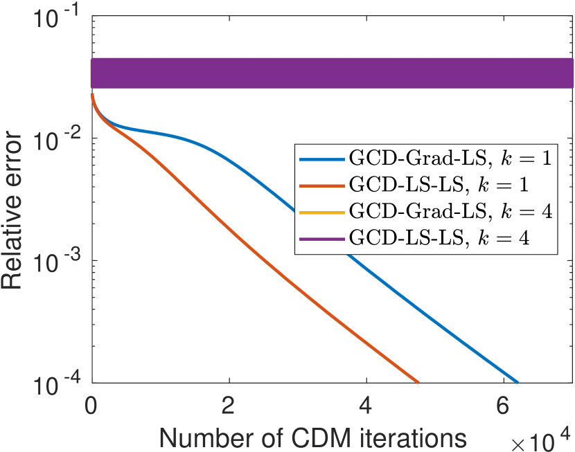
(a) The non-convergence behavior of greedy CDMs on $A_{108}$ with $k=4$ comparing with convergent greedy CDMs with $k=1$. The initial vector is $e_{1}$.

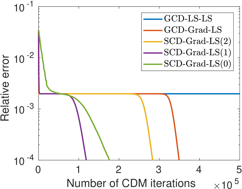
(b) The convergence behavior of greedy CDMs and stochastic CDMs on $A_{108}-100I$. The initial vector has $100$ non-zero entries on random coordinates.

Figure 1: Convergence behavior of greedy coordinate-wise methods vs stochastic coordinate-wise methods. Both (a) and (b) demonstrate the convergence behavior for solving (2) and the matrix $A_{108}$ is a random matrix of size 5000 with largest eigenvalue being 108 and other eigenvalue equally distributed in $[1,100)$. Note that we shift the matrix in (b) as $A_{108}-100I$ so that the only saddle point is the origin.

5.1 SCD-Grad-vecLS and SCD-Grad-LS

Input: Symmetric matrix $A\in\mathbb{R}^{n\times n}$; initial vector ${x}^{(0)}$; probability power $t$; number of coordinates $k$.

1:  ${z}^{(0)}=A{x}^{(0)}$

2:  $\ell=0$

3:  while (not converged) do

4:     $\nu=\norm{{x}^{(\ell)}}^{2}$

5:     for $j=1,2,\dots,n$ do

6:        ${c}^{(\ell)}_{j}=\nu{x}^{(\ell)}_{j}-{z}^{(\ell)}_{j}$

7:     end for

8:     Sample $k$ coordinates with probability proportional to $\absolutevalue{{c}^{(\ell)}}^{t}$, denote it as $\Omega$

9:     Solve (21) with the root picking strategy for $\alpha_{\ell}$

10:     ${x}^{(\ell+1)}_{j}=\begin{cases}{x}^{(\ell)}_{j}+\alpha_{\ell}\nabla_{j}f\bigl{(}{x}^{(\ell)}\bigr{)},&j\in\Omega\\ {x}^{(\ell)}_{j},&j\not\in\Omega\end{cases}$

11:     ${z}^{(\ell+1)}={z}^{(\ell)}+A_{:,\Omega}\bigl{(}{x}^{(\ell+1)}_{\Omega}-{x}^{(\ell)}_{\Omega}\bigr{)}$

12:     $\ell=\ell+1$

13:  end while

Algorithm 5 SCD-Grad-vecLS for LEVP

The first stochastic coordinate-wise descent method we consider is SCD-Grad-vecLS as in Algorithm 5. SCD-Grad-vecLS is a stochastic version of GCD-Grad-LS: Instead of picking the coordinate with largest magnitude in ${c}^{(\ell)}_{j}$, we sample $k$ coordinates with probability proportional to $\bigl{\lvert}{c}^{(\ell)}_{j}\bigr{\rvert}^{t}$ for $t\geq 0$ and the set of sampled indices is denoted as $\Omega$, where as in GCD-Grad-LS in Section 4.1, ${c}^{(\ell)}$ is proportional to the gradient vector, $\nabla f({x}^{(\ell)})$. Hence the sampling strategy here is equivalent to sampling with probability proportional to the $t$-th power of the absolute value of the gradient vector. Through the similar derivation as in Section 4, we can show that the exact line search can also be conducted along a given search direction. We denote the line search objective function as $h(\alpha)=f\bigl{(}{x}^{(\ell)}+\alpha v\bigr{)}=f\bigl{(}{x}^{(\ell)}+\alpha\sum_{j\in\Omega}\nabla_{j}f\bigl{(}{x}^{(\ell)}\bigr{)}e_{j}\bigr{)}$, where $v=\sum_{j\in\Omega}\nabla_{j}f\bigl{(}{x}^{(\ell)}\bigr{)}e_{j}$ defines the search direction. Function $h(\alpha)$ is again a quartic polynomial of $\alpha$. All candidates of optimal $\alpha$ are roots of the cubic polynomial,

$$\begin{split}\frac{\,\mathrm{d}h}{\,\mathrm{d}\alpha}(\alpha)=&4\norm{v_{\Omega}}^{4}\alpha^{3}+12\left(v_{\Omega}^{\top}{x}^{(\ell)}_{\Omega}\right)\norm{v_{\Omega}}^{2}\alpha^{2}\\ &+4\left(\nu\norm{v_{\Omega}}^{2}+2\left(v_{\Omega}^{\top}{x}^{(\ell)}_{\Omega}\right)^{2}-v_{\Omega}^{\top}A_{\Omega,\Omega}v_{\Omega}\right)\alpha+4\nu\left(v_{\Omega}^{\top}{x}^{(\ell)}_{\Omega}\right)-4v_{\Omega}^{\top}{z}^{(\ell)}_{\Omega}=0,\\ \end{split}$$ (21)

where $\nu=\norm{{x}^{(\ell)}}^{2}$. We notice that all coefficients in (21), given $\nu$, can be computed in $O(k^{2})$ operations for $k$ being the number of indices in $\Omega$. Hence all candidates of the optimal $\alpha$ can be obtained in $O(k^{2})$ operations. Analog to Section 4, we adopt the root picking strategy to find the optimal $\alpha$ which has lowest function value. We conclude that the optimal $\alpha$ is achievable in $O(k^{2})$ operations given pre-calculated $\nu$. Algorithm 5 describes the steps in detail.

Input: Symmetric matrix $A\in\mathbb{R}^{n\times n}$; initial vector ${x}^{(0)}$; probability power $t$; number of coordinates $k$.

1:  ${z}^{(0)}=A{x}^{(0)}$

2:  $\ell=0$

3:  while (not converged) do

4:     $\nu=\norm{{x}^{(\ell)}}^{2}$

5:     for $j=1,2,\dots,n$ do

6:        ${c}^{(\ell)}_{j}=\nu{x}^{(\ell)}_{j}-{z}^{(\ell)}_{j}$

7:     end for

8:     Sample $k$ coordinates with probability proportional to $\bigl{|}{c}^{(\ell)}\bigr{|}^{t}$; denote $\Omega$ the sampled index set

9:     for $j\in\Omega$ do

10:        $p_{j}=\nu-\bigl{(}{x}^{(\ell)}_{j}\bigr{)}^{2}-A_{j,j}$

11:        $q_{j}=A_{j,j}{x}^{(\ell)}_{j}-{z}^{(\ell)}_{j}$

12:        Solve $\alpha_{j}^{3}+p_{j}\alpha_{j}+q_{j}=0$ for real $\alpha_{j}$

13:     end for

14:     ${x}^{(\ell+1)}_{j}=\begin{cases}{x}^{(\ell)}_{j}+\alpha_{j},&j\in\Omega\\ {x}^{(\ell)}_{j},&j\not\in\Omega\end{cases}$

15:     ${z}^{(\ell+1)}={z}^{(\ell)}+A_{:,\Omega}\bigl{(}{x}^{(\ell+1)}_{\Omega}-{x}^{(\ell)}_{\Omega}\bigr{)}$

16:     $\ell=\ell+1$

17:  end while

Algorithm 6 SCD-Grad-LS for LEVP

One drawback of Algorithm 5 is that the exact line search relies on all selected coordinates, which is unsuitable for asynchronous implementation. Here we propose an aggressive SCD method, SCD-Grad-LS, which can be implemented in an asynchronized fashion. The method combines the coordinate picking strategy in SCD-Grad-vecLS and coordinate updating strategy in GCD-Grad-LS. But the updating strategy in SCD-Grad-LS updates each coordinate with the coordinate-wise exact line search independently and can be delayed. Algorithm 6 is the pseudo code of SCD-Grad-LS.

Updating $k>1$ coordinates independently as in Algorithm 6 does not have guarantee of convergence. When $k$ is large or $t$ is large such that the same coordinate is updated multiple times, we do observe non-convergent behavior of the iteration in practice. However, as shown in the numerical results, when $k$ is relatively small compared to $n$ and $t=1,2$, SCD-Grad-LS, on average, requires about a fraction of $1/k$ number of iterations. There exists a fix to guarantee the convergence for any $k>1$. Instead of updating as ${x}^{(\ell+1)}={x}^{(\ell)}+\sum_{j\in\Omega}\alpha_{j}e_{j}$, we update as

$${x}^{(\ell+1)}={x}^{(\ell)}+\frac{1}{k}\sum_{j\in\Omega}\alpha_{j}e_{j},$$ (22)

where $\alpha_{j}$ is the optimal step size in $j$-th coordinate as in (10). Such a change enables convergence but usually increases the iteration number by a factor of $k$ if both cases converge.

In the sampling procedure of stochastic CDMs, there are two ways of sampling, sampling with replacement and sampling without replacement. We claim that when $k\ll n$ and the variance of $\absolutevalue{{c}^{(\ell)}}^{t}$ is small, sampling with or without replacement behaves very similarly. While, for $\absolutevalue{{c}^{(\ell)}}^{t}$ with large variance or $k\approx n$, these two sampling strategies behave drastically differently. For example, when $t\rightarrow\infty$, probability proportional to $\absolutevalue{{c}^{(\ell)}}^{t}$ becomes an indicator vector on a single coordinate (assuming non-degeneracy). Sampling with replacement results a set $\Omega$ of $k$ same indices, whereas sampling without replacement results a set of $k$ different indices corresponding to the largest $k$ entries in $\absolutevalue{{c}^{(\ell)}}$. In the analysis below, we prove the local convergence analysis of the Algorithm 5 and Algorithm 6 when $k=1$ (the two algorithms are equivalent when $k=1$). Similar but more complicated analysis could be done for $k\geq 1$ when sampling with replacement is adopted and the modified updating strategy (22) is adopted in Algorithm 6.

5.2 Local convergence of stochastic coordinate-wise descent method

In this section, we analyze the convergence properties of stochastic coordinate-wise descent methods for SCD-Grad-LS. We will present the analysis for a general strongly convex objective function with Lipschitz continuous gradient. The analysis uses the following notations and definitions. We take

$$B^{\pm}=\Set{y}{\norm{y\mp\sqrt{\lambda_{1}}v_{1}}\leq\frac{1}{30}\frac{\min(2\lambda_{1},\lambda_{1}-\lambda_{2})}{\sqrt{\lambda_{1}}}}$$ (23)

as two neighborhoods around global minimizers $\pm\sqrt{\lambda_{1}}v_{1}$ respectively.

Definition 5.1 (Coordinate-wise Lipschitz continuous).

Let a function $g(x):\mathbb{S}\mapsto\mathbb{R}$ be continuously differentiable. The gradient of the function $\nabla g(x)$ is coordinate-wise Lipschitz continuous on $\mathbb{S}$ if there exists a positive constant $L$ such that,

$$\absolutevalue{\nabla_{i}g(x+\alpha e_{i})-\nabla_{i}g(x)}\leq L\absolutevalue{\alpha},\quad\forall\,x,x+\alpha e_{i}\in\mathbb{S}\text{ and }i=1,2,\dots,n.$$ (24)

Compared to the usual Lipschitz constant of $\nabla g(x)$, denoted as $L_{g}$, we have the relation, $L\leq L_{g}$. If $g(x)$ is further assumed to be convex, then we have $L_{g}\leq nL$. If $g(x)$ is twice-differentiable, Definition 5.1 is equivalent to $\absolutevalue{e_{i}^{\top}\nabla^{2}g(x)e_{i}}\leq L$ for all $i=1,2,\dots,n$ and $x\in\mathbb{S}$. An important consequence of a coordinate-wise Lipschitz continuous function $g(x)$ is that

$$g(x+\alpha e_{i})\leq g(x)+\nabla_{i}g(x)\alpha+\frac{L}{2}\alpha^{2},\quad\forall\,x\in\mathbb{S}\text{ and }x+\alpha e_{i}\in\mathbb{S}.$$ (25)

The following lemma extends [21, Lemma A.3] to objective function $f(x)$ with matrix $A$ satisfying Assumption A.

Lemma 5.2.

Function $f(x)$ defined in (2) is a continuously differentiable function. Further the gradient function $\nabla f(x)$ is coordinate-wise Lipschitz continuous on either $B^{+}$ or $B^{-}$ with constant $L=12\lambda_{1}+2\min(2\lambda_{1},\lambda_{1}-\lambda_{2})+4\max_{i}\absolutevalue{A_{i,i}}$.

Definition 5.3 (strongly $\norm{\cdot}_{p}$-convexity).

Let a function $g(x):\mathbb{S}\mapsto\mathbb{R}$ be continuously differentiable. It is said to be strongly $\norm{\cdot}_{p}$-convex, if there exists a constant $\mu_{p}>0$ such that

$$g(y)\geq g(x)+\nabla g(x)^{\top}(y-x)+\frac{\mu_{p}}{2}\norm{y-x}_{p}^{2},\quad\forall x,y\in\mathbb{S}.$$ (26)

Throughout the paper, we assume $p\geq 1$ in the definition. Definition 5.3 is a generalized version of the traditional strong convexity, which corresponds to $p=2$ case.

Combine (26) with the equivalence of different norms in finite dimensional vector space, we obtain for any $p\geq q\geq 1$

$$\begin{split}g(y)&\geq g(x)+\nabla g(x)^{\top}(y-x)+\frac{\mu_{p}}{2}\norm{y-x}_{p}^{2}\\ &\geq g(x)+\nabla g(x)^{\top}(y-x)+n^{\nicefrac{{2}}{{p}}-\nicefrac{{2}}{{q}}}\frac{\mu_{p}}{2}\norm{y-x}_{q}^{2},\quad\forall x,y\in\mathbb{S}.\end{split}$$ (27)

Therefore, if $g(x)$ is a strongly $\norm{\cdot}_{p}$-convex function with constant $\mu_{p}$, then $g(x)$ is a strongly $\norm{\cdot}_{q}$-convex function with constant $\mu_{q}\geq n^{\nicefrac{{2}}{{p}}-\nicefrac{{2}}{{q}}}\mu_{p}$, which is equivalent to $n^{\nicefrac{{2}}{{q}}}\mu_{q}\geq n^{\nicefrac{{2}}{{p}}}\mu_{p}$. On the other hand side, using the inequality of vector norm together with (26), we obtain for any $p\geq q\geq 1$,

$$\begin{split}g(y)&\geq g(x)+\nabla g(x)^{\top}(y-x)+\frac{\mu_{q}}{2}\norm{y-x}_{q}^{2}\\ &\geq g(x)+\nabla g(x)^{\top}(y-x)+\frac{\mu_{q}}{2}\norm{y-x}_{p}^{2},\quad\forall x,y\in\mathbb{S}.\end{split}$$ (28)

Therefore, if $g(x)$ is a strongly $\norm{\cdot}_{q}$-convex function with constant $\mu_{q}$, then $g(x)$ is a strongly $\norm{\cdot}_{p}$-convex function with constant $\mu_{p}\geq\mu_{q}$. Putting two parts together, we have the following inequalities of $\mu_{p}$ and $\mu_{q}$

$$n^{\nicefrac{{2}}{{p}}-\nicefrac{{2}}{{q}}}\mu_{p}\leq\mu_{q}\leq\mu_{p},$$ (29)

where $p\geq q\geq 1$.

Lemma 5.4.

Function $f(x)$ defined in (2) is strongly $\norm{\cdot}_{2}$-convex on either $B^{+}$ or $B^{-}$ with constant $\mu_{2}=3\min(2\lambda_{1},\lambda_{1}-\lambda_{2})$, and hence, there exists $\mu_{p}$ such that $f(x)$ is strongly $\norm{\cdot}_{p}$-convex for any $p\geq 1$.

The proof of the strongly $\norm{\cdot}_{2}$-convexity in Lemma 5.4 follows an extension of the proof of Lemma A.2 in [21], where the minimum eigenvalue of the Hessian matrix is modified according to the assumption of the matrix $A$. Combining with (29), we have the existence of $\mu_{p}$ for all $p\geq 1$.

$B^{+}$ and $B^{-}$ are two disjoint 2-norm ball around global minimizers. Next we define two sublevel sets $D^{+}$ and $D^{-}$, contained in $B^{+}$ and $B^{-}$ respectively as

$$D^{\pm}=\Set{x\in B^{\pm}}{f(x)\leq\min_{y\in\partial B^{\pm}}f(y)},$$ (30)

where $\partial B^{\pm}$ denote the boundary of $B^{\pm}$. Obviously, two global minimizers lie in $D^{\pm}$ respectively, i.e., $\pm\sqrt{\lambda_{1}}v_{1}\in D^{\pm}$. Lemma 5.5 shows monotonic decay property of the iteration defined by Algorithm 6 once the iterations falls in $D^{\pm}$. It also shows that $D^{+}\cup D^{-}$ is a contraction set for the iteration.

Lemma 5.5.

Consider function $f(x)$ as defined in (2) and the iteration follows Algorithm 6 with $k=1$. For any ${x}^{(\ell)}\in D^{+}\cup D^{-}$, we have

$$f\bigl{(}{x}^{(\ell+1)}\bigr{)}\leq f\bigl{(}{x}^{(\ell)}\bigr{)}-\frac{1}{2L}\left(\nabla_{j_{\ell}}f\bigl{(}{x}^{(\ell)}\bigr{)}\right)^{2},$$ (31)

where $j_{\ell}$ is the index of the coordinate being picked. Moreover, we have ${x}^{(\ell+1)}\in D^{+}\cup D^{-}$.

The proof of Lemma 5.5 can be found in Appendix B.

In Algorithm 6, we notice that the iteration of ${x}^{(\ell)}$ in the SCD-Grad-LS samples coordinate $j$ with probability proportional to $\absolutevalue{\nabla_{j}f\left({x}^{(\ell)}\right)}^{t}$ for some non-negative power $t$. In the following lemma and theorem, we adopt notation $f^{*}$ as the minimum of the function and $X^{*}$ be the set of minimizers, i.e., $X^{*}=\Set{\pm\sqrt{\lambda_{1}}v_{1}}$. A distance function between two sets or between a point and a set is defined as, $\mathrm{dist}\bigl{(}S_{1},S_{2}\bigr{)}=\min_{x\in S_{1},y\in S_{2}}\norm{x-y}$.

Lemma 5.6.

Consider function $f(x)$ as defined in (2) and the iteration follows Algorithm 6 with $k=1$. For any ${x}^{(\ell)}\in D^{+}\cup D^{-}$,

$$\mathbb{E}\bigl{[}f\bigl{(}{x}^{(\ell+1)}\bigr{)}\mid{x}^{(\ell)}\bigr{]}-f^{*}\leq\left(1-\frac{\mu_{q}}{Ln^{2-\frac{2}{q}}}\right)\left(f\bigl{(}{x}^{(\ell)}\bigr{)}-f^{*}\right),$$ (32)

where $q=\frac{t+2}{t+1}$.

The proof of Lemma 5.6 can be found in Appendix B.

Theorem 4.

Consider function $f(x)$ as defined in (2) and the iteration follows Algorithm 6 with $k=1$. For any ${x}^{(0)}\in D^{+}\cup D^{-}$,

$$\mathbb{E}\bigl{[}f\bigl{(}{x}^{(\ell)}\bigr{)}\mid{x}^{(0)}\bigr{]}-f^{*}\leq\left(1-\frac{\mu_{q}}{Ln^{2-\frac{2}{q}}}\right)^{\ell}\left(f\bigl{(}{x}^{(0)}\bigr{)}-f^{*}\right),$$ (33)

where $q=\frac{t+2}{t+1}$. Moreover,

$$\mathbb{E}\bigl{[}\mathrm{dist}\bigl{(}{x}^{(\ell)},X^{*}\bigr{)}^{2}\mid{x}^{(0)}\bigr{]}\leq\frac{2}{\mu_{2}}\left(1-\frac{\mu_{q}}{Ln^{2-\frac{2}{q}}}\right)^{\ell}\left(f\bigl{(}{x}^{(0)}\bigr{)}-f^{*}\right).$$ (34)

The proof of Theorem 4 can be found in the Appendix B. Theorem 4 is slightly more complicated than Lemma 5.6 since Algorithm 6 adopts the exact line search and there are two sublevel sets $D^{\pm}$ for the non-convex objective function $f(x)$. The iteration ${x}^{(\ell)}$ might jump between the two sets. The monotonicity of the exact line search is the key to extend Lemma 5.6 to Theorem 4.

Remark 5.7.

According to Theorem 4, the convergence rate depends on $n^{\nicefrac{{2}}{{q}}}\mu_{q}$, which depends on $q$ and hence $t$. The right side of (29) indicates that, for a problem such that $\mu_{1}=\mu_{q}=\mu_{2}$, the convergence rate of $q=1\Leftrightarrow t=\infty$ is $n$ times larger than that of $q=2\Leftrightarrow t=0$. This means that greedy CDM could be potentially $n$ times faster than stochastic CDM with uniform sampling. According to the left side of inequality (29), for $p\geq q$, we have $n^{\nicefrac{{2}}{{p}}}\mu_{p}\leq n^{\nicefrac{{2}}{{q}}}\mu_{q}$, which means the convergence rate of $q$ is equal to or faster than that of $p$. In terms of $t$, we conclude that the convergence rate of smaller $t$ is smaller than that of larger $t$ and larger $t$ potentially leads to faster convergence.

Remark 5.8.

For a fair comparison between CDMs with traditional methods such as gradient descent, we should take $n$ iterations of CDM and compare it against a single iteration of gradient descent since one iteration of CDM only updates one coordinate whereas one iteration of gradient descent updates $n$ coordinates. Under such a setting, Theorem 4 implies that

$$\mathbb{E}\bigl{[}f\bigl{(}{x}^{(n\ell)}\bigr{)}\mid{x}^{(0)}\bigr{]}-f^{*} \leq\left(1-\frac{\mu_{q}}{Ln^{2-\frac{2}{q}}}\right)^{n\ell}\left(f\bigl{(}{x}^{(0)}\bigr{)}-f^{*}\right)$$

$$\leq\bigl{(}e^{-\frac{\mu_{q}}{L}n^{\frac{2}{q}-1}}\bigr{)}^{\ell}\left(f\bigl{(}{x}^{(0)}\bigr{)}-f^{*}\right),$$

and

$$\mathbb{E}\bigl{[}\mathrm{dist}\bigl{(}{x}^{(n\ell)},X^{*}\bigr{)}^{2}\mid{x}^{(0)}\bigr{]}\leq\frac{2}{\mu_{2}}\bigl{(}e^{-\frac{\mu_{q}}{L}n^{\frac{2}{q}-1}}\bigr{)}^{\ell}\left(f\bigl{(}{x}^{(0)}\bigr{)}-f^{*}\right).$$

For uniform sampling, $t=0$ and $q=2$, the decreasing factor is $e^{-\frac{\mu_{q}}{L}n^{\frac{2}{q}-1}}=e^{-\frac{\mu_{2}}{L}}$, which is independent of $n$. This result implies Algorithm 6 with uniform sampling has the same convergence rate as gradient descent. Combining with Remark 5.7, we conclude that Algorithm 6 with arbitrary $t\geq 0$ converges at least as fast as gradient descent.

Remark 5.9.

If we extend Definition 5.1 to multi-coordinate Lipschitz continuity, and assume $f(x)$ is multi-coordinate Lipschitz continuous with $\widetilde{L}$, a natural extension of Theorem 4 would follow. Unfortunately, if the coordinates are sampled independently, in an extreme case when $k$ same coordinates are sampled, the convergence rate would be the same as that in Theorem 4. In the end, the convergence rate would not be improved and could be even worse. This is similar to the argument of CDM vs. full gradient descent method. In practice, when $k$ is not too large, and the sampled coordinates are distinct, we do observe $k$-fold speed-up of the iterations. This observation suggests that the convergence rate in Theorem 4 is not sharp for $k>1$.

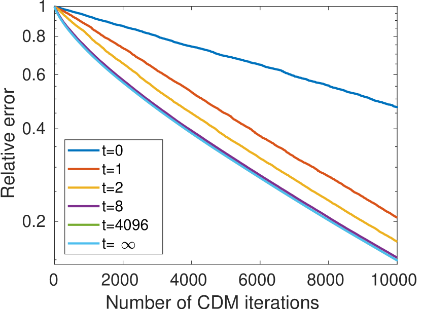
(a) single-coordinate updating

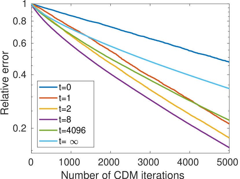
(b) double-coordinate updating

Figure 2: Convergence behavior of SCD-Grad-Grad method with different choice of $t$. The axis of iterations on (a) is twice as long as that in (b).

Combining Theorem 4 together with the monotonicity of $\mu_{q}$ as (29) shows that the lower bound of the convergence rate increases monotonically as $q$ decreases. In terms of $t$, the larger $t$ corresponds to smaller $q$ which leads to larger $\mu_{q}$ for $q=\frac{t+2}{t+1}$. Here we would like to argue that the equality of (29) is achievable which demonstrates the power of CDMs with such a sampling strategy. Consider a simple example $f(x)=\norm{Ax-b}^{2}$ for $A$ being a diagonal matrix with diagonal entries $A_{i,i}=1000$, $i=1,2,\dots,4999$, $A_{5000,5000}=1$ and $b=\begin{bmatrix}0&\cdots&0&1\end{bmatrix}^{\top}$ being a column vector of size $5000$. Through elementary calculations, we can show that $\nabla^{2}f(x)=2A^{2}$, $\mu_{0}=2$ and $\mu_{\infty}\approx 1.99$. Therefore all $\mu_{t}$ lies in the small interval $[1.99,2]$ and different choice of $t$ would lead to different rate of convergence. We minimize $f(x)$ using the SCD-Grad-Grad method. The step size is fixed to be $10^{-6}$ and the initial vector is chosen randomly. Figure 2 (a) demonstrates the first $10^{4}$ iterations of the SCD-Grad-Grad with different choice of $t$. The relative error is defined to be $\bigl{(}f\bigl{(}{x}^{(\ell)}\bigr{)}-f\bigl{(}x^{*}\bigr{)}\bigr{)}/f\bigl{(}{x}^{(0)}\bigr{)}$. Clearly, different choice of $t$ leads to different convergence rates. And we also notice that the most significant improvement appears when increasing $t$ from 0 to 1, which implies that sampling with respect to magnitude of gradient is much better than sampling uniformly. In Figure 2 (a), the line with $t=4096$ and that with $t=\infty$ overlap.

According to either Theorem 4 or Figure 2 (a), it is convincing that for single-coordinate updating CDM, picking the index with largest gradient magnitude should be the optimal strategy. Figure 2 (b) investigates the case with double-coordinate updating, i.e., sample two coordinates independently and update two entries simultaneously in every iteration. Comparing Figure 2 (a) and (b), we notice for small $t$, double-coordinate updating strategy almost reduces the required number of iterations by half. As $t\rightarrow\infty$, the sampling approaches choosing the coordinate with largest gradient magnitude with probability $1$. Sampling two coordinates independently thus results in sampling the same index twice and the iteration behaves similar to the single-coordinate updating CDM. Readers may argue that we should sample without replacement or sampling two indices with two largest gradient magnitudes and updating accordingly. However, when the objective function is non-convex, for example, the objective function $f(x)$ defined in (2), the iteration usually stick in the middle of iteration (see Figure 1 (a)).

Remark 5.10 (Local convergence of greedy coordinate-wise descent method).

The local convergence analysis of SCDMs can be extended to the greedy coordinate-wise descent methods. GCD-Grad-LS as in Algorithm 4 is a special case of SCD-Grad-LS with $t=\infty$ and $k=1$. Hence Theorem 4 proves the local convergence of the GCD-Grad-LS with $q=1$.

GCD-LS-LS as in Algorithm 4 conducts optimal coordinate-wise descent every iteration. Therefore, for GCD-LS-LS, Lemma 5.5 can be proved for any index of coordinate $j$ and then Lemma 5.6 holds for $q=1$. The modified lemmas lead to the following corollary.

Corollary 5.11.

Consider function $f(x)$ as defined in (2) and the iteration follows Algorithm 4. For any ${x}^{(0)}\in D^{+}\cup D^{-}$,

$$\mathbb{E}\bigl{[}f\bigl{(}{x}^{(\ell)}\bigr{)}\mid{x}^{(0)}\bigr{]}-f^{*}\leq\left(1-\frac{\mu_{1}}{L}\right)^{\ell}\left(f\bigl{(}{x}^{(0)}\bigr{)}-f^{*}\right).$$ (35)

Moreover,

$$\mathbb{E}\bigl{[}\mathrm{dist}\bigl{(}{x}^{(\ell)},X^{*}\bigr{)}^{2}\mid{x}^{(0)}\bigr{]}\leq\frac{2}{\mu_{2}}\left(1-\frac{\mu_{1}}{L}\right)^{\ell}\left(f\bigl{(}{x}^{(0)}\bigr{)}-f^{*}\right).$$ (36)

The local convergence of GCD-Grad-LS and GCD-LS-LS are achieveable, while the global convergences are so far still open. Numerically, both methods converge to global minima for most the cases we tested.

Remark 5.12 (Convergence behavior in non-convex area).

We demonstrate one example such that the stochastic CDMs outperforms greedy CDMs even all methods are conducting single coordinate updating. We generate a random matrix $A_{108}-100I$ of size 5000, whose the largest eigenvalue is 8 and other eigenvalues are distributed equally on $[-99,0)$. According to Lemma 2.5, $0$ is the only strict saddle point of the problem. If all methods start with a sparse initial vector, in this problem, they all converge to the strict saddle point first, and then escape from it. Figure 1 (b) shows the convergence behavior of five methods ordered by the degree of greediness. The horizontal line is the relative error at the strict saddle point 0. As we can see that it takes more time for greedier method to escape from the saddle point. And although SCD-Grad-LS(0) escape from the saddle point fastest, but the overall performance is worse than SCD-Grad-LS(1). This motivates us to apply SCD-Grad-LS with small $t$ in practice. Such methods are almost as efficient as the greedy methods, as shown in Figure 2, they are also robust to non-convex objective functions near saddle points.

6 Numerical results

In this section, we perform numerical tests of the methods mentioned in previous sections on two different kinds of matrices. The first numerical test calculates the largest eigenvalue of a random symmetric dense matrix, where we have control of the difficulty of the problems. The leading eigenvector is evenly distributed among all the entries. The second test calculates the ground energy and ground state of the two dimensional (2D) Hubbard model, which is one of our target applications for the quantum many-body calculation. The ground state problem in quantum many-body system is equivalent to find the smallest eigenvalue of a huge sparse symmetric matrix, with each coordinate representing the coefficient of a Slater determinant. Although the eigenvector in this example is dense, it is also ‘sparse’ in some sense, which means a great majority of the entries is close to zero. Without eigenvector compression, for the quantum many-body calculation, the state-of-the-art algorithms are in fact variants of power iterations. Hence in this paper, we compare coordinate-wise methods against power method as it is a simple baseline algorithm. Due to the nature of the problem, it is anticipated that CDMs will have much better performance over the traditional power method.

Three quantities are used to measure the convergence of the methods: the square root of the relative error of the objective function value (2), the relative error of the eigenvalue and the tangent of the angle between ${x}^{(\ell)}$ and the eigenvector. The square root of the relative error of the objective function value is defined as

$$\epsilon_{\mathrm{obj}}=\sqrt{\frac{f\bigl{(}x^{(\ell)}\bigr{)}-f^{*}}{f^{*}}},$$ (37)

where $f^{*}$ denotes the minimum of $f(x)$. Since $f^{*}$ is on the scale of $\lambda_{1}^{2}$, we use the square root of the relative error of the objective function which is on the same scale as $\lambda_{1}$. To estimate the eigenvalue, we use

$$E=\frac{x_{*}^{\top}Ax^{(\ell)}}{x_{*}^{\top}x^{(\ell)}},$$ (38)

where $x_{*}$ is the reference vector that overlaps with the eigenvector $v_{1}$. In our test, $x_{*}$ is a unit vector and will be specified later. This estimator is referred as the projected energy in the context of quantum chemistry. Thus the relative error is define by

$$\epsilon_{\mathrm{energy}}=\frac{\absolutevalue{E-\lambda_{1}}}{\absolutevalue{\lambda_{1}}}.$$ (39)

Last,

$$\epsilon_{\mathrm{tan}}=\tan{\theta(v^{(\ell)},v_{1})}$$ (40)

is used to measure the convergence of the eigenvector.

The number of matrix column evaluation is used to measure the efficiency of the methods. There are several reasons why the number of matrix column evaluation is a good measure. First it is independent of the computation environment. Second we assume the evaluation of matrix column is the most expensive step. It is usually true in quantum many-body calculation in chemistry (full configuration interaction method) because the matrix is too large to be stored, the evaluation has to be on-th-fly and the evaluation of each entry is relatively expensive. Third, it can be used to compare with other related methods.

All methods are implemented and tested in MATLAB R2017b. The exact eigenvalue and eigenvector of each problem are calculated by the “eigs” function in Matlab with high precision.

6.1 Dense random matrices

Table 3: Performance of various algorithms for $A_{108}$

Method	$k$	Min Iter Num	Med Iter Num	Max Iter Num	Total Col Access
PM	5000	-	135	-	675000
CPM	1	-	309085	-	309085
CPM	4	-	75829	-	303316
CPM	16	-	18809	-	300944
SI-GSL($\lambda_{1}$)	1	-	260000	-	260000
SI-GSL($1.5\lambda_{1}$)	1	-	1002283	-	1002283
Grad-vecLS	5000	-	80	-	400000
GCD-Grad-LS	1	-	109751	-	109751
GCD-LS-LS	1	-	100464	-	100464
SCD-Grad-vecLS(0)	4	86054	94837	128467	379348
SCD-Grad-vecLS(0)	16	21409	24066	30850	385056
SCD-Grad-vecLS(1)	4	36081	40866	52279	163464
SCD-Grad-vecLS(1)	16	9225	10205	11934	163280
SCD-Grad-vecLS(2)	4	29867	33538	45480	134152
SCD-Grad-vecLS(2)	16	7417	8334	11410	133344
SCD-Grad-LS(0)	1	342945	377783	483842	377783
SCD-Grad-LS(0)	4	86241	96074	150090	384296
SCD-Grad-LS(0)	16	21952	24487	31313	391792
SCD-Grad-LS(1)	1	146161	166415	223471	166415
SCD-Grad-LS(1)	4	38034	41773	53257	167092
SCD-Grad-LS(1)	16	9207	10479	15063	167664
SCD-Grad-LS(2)	1	120411	136468	177161	136468
SCD-Grad-LS(2)	4	30200	34091	44993	136364
SCD-Grad-LS(2)	16	7583	8631	11415	138096

We first show the advantage of the coordinate-wise descent methods over power method on dense random matrices. All matrices tested in this section involve symmetric matrices of size 5000 with random eigenvectors, i.e.,

$$A_{\lambda_{1}}=Q\begin{bmatrix}\lambda_{1}&&&\\ &\lambda_{2}&&\\ &&\ddots&\\ &&&\lambda_{5000}\end{bmatrix}Q^{\top},$$ (41)

where $\lambda_{2},\dots,\lambda_{5000}$ are equally distributed on $[1,100)$ and $Q$ is a random unitary matrix generated by a QR factorization of a random matrix with each entry being Gaussian random number. We use $\lambda_{1}$ to control the difficulty of the problem. In particular, we tested three matrices $A_{108}$, $A_{101}$, and $A_{108}+1000I$. The last one is a shifted version of $A_{108}$. It is obvious that $A_{108}+1000I$ is more difficult than $A_{108}$ for power methods. For the optimization problem (2), it is also more difficult since the landscape of the objective function becomes steeper. While, in practice, CDMs for the optimization problem is less sensitive to the shift. In this section, all results are reported in terms of number of column accesses, converging to $10^{-6}$ under the measure of $\epsilon_{\mathrm{obj}}$. For non-stochastic methods, we report the number of column accesses from a single run and reported in the column named “Med Iter Num”. While, for stochastic methods, we report the minimum, medium, and maximum numbers of iterations from 100 runs. In all tables, the column named “Total Col Access” provides the total number of matrix column evaluation, which is calculated as the product of number of coordinates updating each iteration, i.e., $k$, and the medium number of iterations. The initial vector of CDM is always chosen to be the unit vector $e_{1}$, with $1$ in the first coordinate and $0$ in all others.

Table 4: Performance of various algorithms for $A_{101}$

Method	$k$	Min Iter Num	Med Iter Num	Max Iter Num	Total Col Access
PM	5000	-	839	-	4195000
CPM	1	-	1899296	-	1899296
CPM	4	-	471779	-	1887116
CPM	16	-	125525	-	2008400
SI-GSL($\lambda_{1}$)	1	-	460000	-	460000
SI-GSL($1.5\lambda_{1}$)	1	-	3972548	-	3972548
Grad-vecLS	5000	-	480	-	2400000
GCD-Grad-LS	1	-	726093	-	726093
GCD-LS-LS	1	-	554521	-	554521
SCD-Grad-vecLS(0)	4	444954	557394	788291	2229576
SCD-Grad-vecLS(0)	16	118259	140177	178029	2242832
SCD-Grad-vecLS(1)	4	207804	253035	389396	1012140
SCD-Grad-vecLS(1)	16	53497	62959	84697	1007344
SCD-Grad-vecLS(2)	4	173455	206857	367199	827428
SCD-Grad-vecLS(2)	16	43618	51701	82524	827216
SCD-Grad-LS(0)	1	1896835	2208812	3279223	2208812
SCD-Grad-LS(0)	4	483657	571571	832675	2286284
SCD-Grad-LS(0)	16	119192	139788	203427	2236608
SCD-Grad-LS(1)	1	871362	1022169	1481621	1022169
SCD-Grad-LS(1)	4	206500	262616	402321	1050464
SCD-Grad-LS(1)	16	54106	63607	94236	1017712
SCD-Grad-LS(2)	1	717007	820728	1205225	820728
SCD-Grad-LS(2)	4	176141	209155	288910	836620
SCD-Grad-LS(2)	16	43237	51768	75115	828288

Table 5: Performance of various algorithms for $A_{108}+1000I$

Method	$k$	Min Iter Num	Med Iter Num	Max Iter Num	Total Col Access
PM	5000	-	1214	-	6070000
CPM	1	-	3338202	-	3338202
CPM	4	-	853724	-	3414896
CPM	16	-	214645	-	3434320
SI-GSL($\lambda_{1}$)	1	-	140000	-	140000
SI-GSL($1.5\lambda_{1}$)	1	-	1409635	-	1409635
Grad-vecLS	5000	-	875	-	4375000
GCD-Grad-LS	1	-	92532	-	92532
GCD-LS-LS	1	-	102098	-	102098
SCD-Grad-vecLS(0)	4	78212	92682	126872	370728
SCD-Grad-vecLS(0)	16	18632	21257	30375	340112
SCD-Grad-vecLS(1)	4	31107	34023	48125	136092
SCD-Grad-vecLS(1)	16	7888	8570	10915	137120
SCD-Grad-vecLS(2)	4	25047	27733	37547	110932
SCD-Grad-vecLS(2)	16	6111	7000	9788	112000
SCD-Grad-LS(0)	1	336724	404492	486490	404492
SCD-Grad-LS(0)	4	88807	100736	127954	402944
SCD-Grad-LS(0)	16	22687	25715	34403	411440
SCD-Grad-LS(1)	1	125623	139462	192680	139462
SCD-Grad-LS(1)	4	31205	34731	54808	138924
SCD-Grad-LS(1)	16	8081	9524	13275	152384
SCD-Grad-LS(2)	1	101177	110757	147548	110757
SCD-Grad-LS(2)	4	25399	31354	52048	125416
SCD-Grad-LS(2)	16	do not converge

Among the methods compared, PM and Grad-vecLS with $k=5000$ update all coordinates per iteration. All other methods are coordinate-wise methods and all of them show speedup. PM converges the slowest. Although the iteration number is small, the cost of each iteration is huge. CPM reduces the cost by half on average, which is a big improvement. Grad-vecLS with $k=5000$ is equivalent to gradient descent with exact line search. Since it updates at the full gradient direction, the cost is also large. SI-GSL($\lambda_{1}$) and SI-GSL($1.5\lambda_{1}$) adopt $\lambda_{1}$ and $1.5\lambda_{1}$ as the estimation of the leading eigenvalue respectively, and other parameters in SI-GSL are set to be the underlying true values. SI-GSL($\lambda_{1}$) in general performs compariable to GCD-Grad-LS and GCD-LS-LS, while SI-GSL($1.5\lambda_{1}$) is siganificantly slower than all optimization based CDMs. The performance of SI-GSL sensitively depends on the provided a priori estimation of the leading eigenvalue, which makes it impractical for our target application settings. The greedy methods GCD-Grad-LS and GCD-LS-LS speed up significantly. They are about six times faster than PM for $A_{108}$ and $A_{101}$. While, for $A_{108}+1000I$, the greedy methods is about 70 times faster. The two greedy methods themselves have similar cost. For the stochastic methods, we use gradient information to pick the coordinates and use vecLS or LS to update. Different probability power $t$ and number of coordinates updated $k$ are tested. With the same parameters, SCD-Grad-vecLS and SCD-Grad-LS share the similar performance. For $t=0$, which is equivalent to uniform sampling, the number of column accesses are almost the same as the steepest gradient descent. It is reasonable since uniform sampling does not pick the important coordinate and should behave similar with the full gradient. For $t=1$ and $t=2$, the speedup is obvious. The performance for different $t$ agrees with Theorem 4, since larger $t$ shows faster convergence. Another thing to notice is that the cost is not influenced by the different choices of $k$ for CPM and SCD. Therefore if we do the real asynchronized version, more speedup can be gained. Moreover, for stochastic CDMs, the variance is not large.

Comparing the performance for $A_{101}$ and $A_{108}$, the numbers of column accesses for $A_{101}$ are approximately six times as many as for $A_{108}$ for all methods. This behavior is anticipated. Comparing $A_{108}$ to $A_{108}+1000I$, we see that PM, CPM and Grad-vecLS slow down significantly by the shift, since the condition number ($\frac{\lambda_{1}}{\lambda_{1}-\lambda_{2}}$ for PM and the condition number of the Hessian for gradient descent) increases. However, all SI-GSL, GCD and SCD methods converge at almost the same speed, or even a little faster.

6.2 Hubbard models

In this test, we calculate the ground energy and ground state of the 2D Hubbard model. The fermion Hubbard model is widely used in condensed matter physics, which models interacting fermion particles in a lattice with the nearest neighbor hopping and on-site interaction. It is defined by the Hamiltonian in the second quantization notation:

$$\hat{H}=-t\sum_{\langle r,r^{\prime}\rangle,\sigma}\hat{c}_{r,\sigma}^{\dagger}\hat{c}_{r^{\prime},\sigma}+U\sum_{r}\hat{n}_{r\uparrow}\hat{n}_{r\downarrow},$$ (42)

where $t$ is the hopping strength and $U$ is the on-site interaction strength. $r,r^{\prime}$ are indexes of sites in the lattice, and $\langle r,r^{\prime}\rangle$ means $r$ and $r^{\prime}$ are the nearest neighbor. The spin $\sigma$ takes value of $\uparrow$ and $\downarrow$. The operators $\hat{c}_{r,\sigma}^{\dagger}$ and $\hat{c}_{r,\sigma}$ are creation and annihilation operators, which create or destroy a fermion at site $r$ with spin $\sigma$. They satisfy the canonical anticommutation relation:

$$\{\hat{c}_{r,\sigma},\hat{c}_{r^{\prime},\sigma^{\prime}}^{\dagger}\}=\delta_{r,r^{\prime}}\delta_{\sigma,\sigma^{\prime}},\qquad\{\hat{c}_{r,\sigma},\hat{c}_{r^{\prime},\sigma^{\prime}}\}=0,\quad\text{and}\quad\{\hat{c}_{r,\sigma}^{\dagger},\hat{c}_{r^{\prime},\sigma^{\prime}}^{\dagger}\}=0,$$

where $\{A,B\}=AB+BA$ is the anti-commutator. $\hat{n}_{r,\sigma}=\hat{c}_{r,\sigma}^{\dagger}\hat{c}_{r,\sigma}$ is the number operator.

When the interaction is not strong, we usually work in the momentum space. Because in the momentum space, the hopping term in the Hamiltonian is diagonalized and the ground state is close to the Hatree-Fock (HF) state. Mathematically speaking, the normalized leading eigenvector $v_{1}$ is close to the unit vector $e_{\mathrm{HF}}$ whose nonzero entry indicates the HF state. The Hamiltonian in momentum space can be written as

$$\hat{H}=t\sum_{k,\sigma}\varepsilon(k)\hat{n}_{k,\sigma}+\frac{U}{N^{\text{orb}}}\sum_{k,p,q}\hat{c}_{p-q,\uparrow}^{\dagger}\hat{c}_{k+q,\downarrow}^{\dagger}\hat{c}_{k,\downarrow}\hat{c}_{p,\uparrow},$$ (43)

where $\varepsilon(k)=-2(\cos(k_{1})+\cos(k_{2}))$ and $N^{\text{orb}}$ is the number of orbitals. In momentum space, $k$ is the wave number and the creation and annihilation operator can be obtained by the transform $\hat{c}_{k,\sigma}=\frac{1}{\sqrt{N^{\text{orb}}}}\sum_{r}e^{ik\cdot r}\hat{c}_{r,\sigma}$.

To study the performance of methods, we test several 2D Hubbard models with different sizes. Here we report the results of two Hubbard models: both of them are on the $4\times 4$ lattice with periodic boundary condition. The hopping strength is $t=1$ and the interaction strength is $U=4$. The first example contains $6$ electrons, with $3$ spin up and $3$ spin down, whereas the second example contains $10$ electrons, with $5$ spin up and $5$ spin down. The properties of the Hamiltonians are summarized in Table 6. The nonzero off-diagonal entries of $H$ take value $\pm\frac{U}{N^{\text{orb}}}=\pm 0.25$, and the diagonal entries distribute in $(-20,30)$ with bell-like shape. From the table we see that the Hamiltonians are indeed sparse. The smallest eigenvalue (Eigenvalues Min) is the ground energy we are to compute, thus the difference between the smallest one and the second smallest one is the eigengap. Since the spectra of $H$ of the two examples live in the interval $(-100,100)$, the matrix $A=100I-H$ is used for calculation such that the smallest eigenvalue of $H$ becomes the largest one of $A$ and $A$ is positive definite. Both the initial vector and the reference vector of the energy estimator are chosen to be $10\,e_{\mathrm{HF}}$ for all calculation, this amounts to an initial guess of eigenvector $e_{\mathrm{HF}}$ with eigenvalue $10^{2}=100$ on the same scale as the diagonal of $A$ (due to the $100I$ shift). Notice that the reference vector has only one nonzero entry, so computing the projected energy is cheap.

Table 6: Properties of the Hubbard Hamiltonian

$H$	Dim	nnz per col			Eigenvalues
		Min	Med	Max	Min	2nd Min	Max
6 electrons	$1.96\times 10^{4}$	$100$	$102$	$112$	$-14.90$	$-14.55$	$20.26$
10 electrons	$1.19\times 10^{6}$	$196$	$202$	$240$	$-19.58$	$-17.08$	$32.73$

For the first example, the $4\times 4$ Hubbard model with $6$ electrons, we run the methods until the relative error of the objective function value $e_{\mathrm{obj}}<10^{-6}$. The result is shown in Table 7.

Table 7: Performance of various algorithms for $4\times 4$ Hubbard model with $6$ electrons

Method	$k$	Min Iter Num	Med Iter Num	Max Iter Num	Total Col Access
PM	19600	-	2255	-	44198000
CPM	1	-	456503	-	456503
CPM	16	-	29293	-	468688
Grad-vecLS	19600	-	361	-	7075600
GCD-Grad-LS	1	-	31997	-	31997
GCD-LS-LS	1	-	30996	-	30996
SCD-Grad-vecLS(1)	4	36966	38763	40224	155052
SCD-Grad-vecLS(1)	16	11490	12115	12644	193840
SCD-Grad-vecLS(1)	32	6283	6642	6991	212544
SCD-Grad-vecLS(2)	4	18934	19260	19613	77040
SCD-Grad-vecLS(2)	16	6438	6547	6652	104752
SCD-Grad-vecLS(2)	32	3880	3946	4002	126272
SCD-Grad-LS(1)	1	117261	120613	123744	120613
SCD-Grad-LS(1)	2	58536	60470	62209	120940
SCD-Grad-LS(1)	4	28716	30152	30918	120608
SCD-Grad-LS(1)	8	13053	15352	20197	122816
SCD-Grad-LS(2)	1	47603	48136	48802	48136
SCD-Grad-LS(2)	2	23789	24059	24399	48118
SCD-Grad-LS(2)	4	do not converge
SCD-Grad-LS(2)	8	do not converge

In Table 7, the second column $k$ is the number of coordinates updated in one iteration. Each stochastic method runs for $100$ times and we report the number of iterations and matrix column accesses, similar to the previous tests.

Since the dimension of the Hubbard model is larger and the eigenvector $v_{1}$ is sparser than that in the first dense matrix example, the advantage of the coordinate-wise methods is more significant. They are $10^{2}$ to $10^{3}$ faster than PM. GCD-Grad-LS and GCD-LS-LS are still the fastest one. Stochastic CDMs also outperform PM and CPM. Comparing with the greedy CDMs, they are about 3-5 times slower, which is more than that in the previous tests.

For the second model with $10$ electrons in the $4\times 4$ grid, we also compare with other methods, such as SCPM (stochastic version of CPM), SCD-Uni-Grad (which samples coordinate uniformly and updates the coordinate as the gradient multiplying a fixed stepsize), CD-Cyc-LS (which picks the coordinate in a cyclic way and updates the coordinate using line search), and SCD-Uni-LS (i.e., SCD-Grad-LS(0)). The step size, if used, is chosen to be $2$. This step size is larger than that in Theorem 2, but numerically the iteration converges. All methods besides PM update single coordinate per iteration and running up to $10^{7}$ column accesses or desired accuracy. Stochastic CDMs sample coordinate with respect to the magnitude of the gradient, i.e., $t=1$. The convergence of the square root of the relative error of objective function value $\epsilon_{\mathrm{obj}}$, eigenvalue estimator $\epsilon_{\mathrm{energy}}$ and eigenvector estimator $\epsilon_{\mathrm{tan}}$ are plotted in Figure 3.

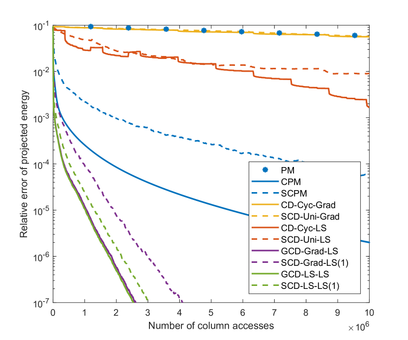
(a) $\epsilon_{\mathrm{energy}}$, Relative error of projected energy

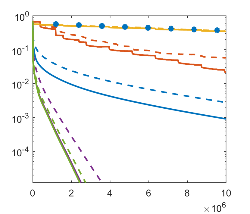
(b) $\epsilon_{\mathrm{tangent}}$, Tangent of angle between $v^{(\ell)}$ and $v_{1}$

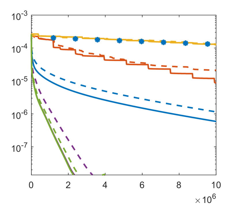
(c) $\epsilon_{\mathrm{obj}}$, Relative error of objective function value

Figure 3: Convergence behavior of the methods for the $4\times 4$ Hubbard model with $10$ electrons. $k=1$ for all methods except PM.

From Figure 3, we see that the convergence of the three error measures share a similar pattern, thus the convergence of one quantity should imply the convergence of the other two in practice. The convergence of all methods tested consist of one or two stages: a possible fast decay followed by linear convergence. We know that both power method (PM) and gradient descent (Grad) converge linearly. In this figure there are only $8$ iterates of PM since each iteration needs the full access of the matrix. CD-Cyc-Grad and SCD-Uni-Grad seem to behave similarly with slow linear decay, which is reasonable since they treat each coordinate equally and should behave similarly as the gradient descent method. CD-Cyc-LS and SCD-Uni-LS also decay linearly, but with a faster rate. This is because updating coordinates by Grad uses the same step size for all coordinates and all iterates, which has to be small thus not optimal. LS always gives the fastest local decay for different coordinates and different iterates. This argument can be confirmed by the sudden-decay-behavior of CD-Cyc-LS. When CD-Cyc-LS updates the important coordinate, it will give a large ‘step size’ and the error drops down rapidly.

All the other methods decay very fast at the beginning, and the common feature is that they pick the coordinates for updating according to their importance, instead of treating them equally. This justifies the motivation of coordinate descent methods. Within $10^{5}$ column accesses, equivalent to $\nicefrac{{1}}{{12}}$ iteration of PM, the projected energy reaches $10^{-2}$ to $10^{-4}$ accuracy. This is really amazing, and agrees with the result of the previous examples. GCD-Grad-LS and GCD-LS-LS behave almost the same and they converge fastest both at the initial stage and the linear convergence stage. The projected energy reaches $10^{-8}$ accuracy when PM only iterates $3$ times. SCD-LS-LS and SCD-Grad-LS also converge fast. The convergence rates of CPM and SCPM are not as fast as SCD-LS-LS and SCG-Grad-LS, but they are still much better than PM.

Comparing between the stochastic CDMs and the greedy CDMs, greedy methods always converge a little faster, such as CD-Cyc-LS versus SCD-Uni-LS and GCD-Grad-LS versus SCD-Grad-LS. This agrees with our theoretical results and previous examples. If more than $1$ coordinate is updated at each iteration, greedy CDMs often get stuck but stochastic CDMs are much less likely. Another thing to mention is that in a small neighborhood of the minimum, updating by LS is almost the same as updating by Grad with some step size depending on the Hessian of the minimum. Thus, updating by Grad could perform as well as LS ideally if there exists a step size which both guarantees the convergence and also converges fast. On the other hand size, LS choose a optimal step size every iteration.

7 Conclusion

We analyze the landscape of the non-convex objective function $f(x)$ of LEVP as (2) and conclude that all local minima of $f(x)$ are global minima. We then investigate CD-Cyc-Grad and prove the global convergence of CD-Cyc-Grad on $f(x)$ almost surely. Through the derivation of the exact line search along a coordinate, GCD-LS-LS is presented as the most greedy CDM and avoids many saddle points of $f(x)$. Finally we propose SCD-Grad-vecLS($t$) and SCD-Grad-LS($t$). The local convergence analysis for these stochastic CDMs shows that convergence rate of either GCD-LS-LS or SCD-Grad-LS($t$) with $t>0$ is provably faster or equal to that of SCD-Uni-LS. And one example as in Figure 1 (b), demonstrates the robustness of the SCD-Grad-LS($t$) with small $t$. Therefore we recommend SCD-Grad-LS(1) as an efficient and robust CDM for LEVP. Numerical results agree with our analysis. The performance of CDMs on a protypical quantum many-body problem of the Hubbard model shows that CDMs has great potential for quantum many-body calculations.

There are several directions worth exploring for future works. Momentum acceleration for coordinate descent [2, 20, 22, 29] can be combined with the proposed methods to potentially accelerate the convergence at least in the local convex area. Also it is of interest to pursue the asynchronous implementation of the proposed methods and prove the convergence property in that setting. Another possible future direction is to employ the sparsity of the matrix into the method such that per-iteration cost could be further reduced. Last but not least, the proposed methods should be extensively tested on other quantum many-body calculations and more other areas whose computational bottlenecks are the LEVP.

Acknowledgments. This work is partially supported by the National Science Foundation under awards OAC-1450280 and DMS-1454939. We thank Stephen J. Wright, Weitao Yang and Wotao Yin for helpful discussions.

Appendix A Proof of Theorem 2

In order to show the global convergence of the CD-Cyc-Grad, we introduce a few definitions and terminologies here. Let $\chi^{s}$ be a set of strict saddle points of $f(x)$, i.e., $\chi^{s}$ is characterized by Lemma 2.5. Let $g_{j}(x)$ be the “coordinate-updating” in Algorithm 2, mapping from ${x}^{(\ell)}$ to ${x}^{(\ell+1)}$ with coordinate $j$, i.e.,

$${x}^{(\ell+1)}=g_{j}({x}^{(\ell)}).$$ (44)

When $n$ steps of updating are composed together, we denote the composed mapping as

$$g=g_{n}\circ g_{n-1}\circ\cdots\circ g_{1}.$$ (45)

The corresponding iteration then is

$${x}^{((k+1)n)}=g({x}^{(kn)}),\qquad k=0,1,2,\dots.$$ (46)

We first establish a few lemmas for the proof of Theorem 2.

Lemma A.1.

Let $R\geq\sqrt{\max_{j}\norm{A_{:,j}}}$ be a constant, $\gamma\leq\frac{1}{4(n+4)R^{2}}$ be the stepsize, and $W_{0}=\left\{x:\norm{x}_{\infty}<R\right\}$ be the set of initial vectors. For any $x^{(0)}\in W_{0}$, and any coordinate index $j$, the following iteration is still in $W_{0}$, i.e.,

$$x^{(1)}=g_{j}(x^{(0)})=x^{(0)}-\gamma\left(-4{z}^{(0)}_{j}+4\norm{x^{(0)}}^{2}{x}^{(0)}_{j}\right)e_{j}\in W_{0},$$ (47)

where $g_{j}$ is defined as (44).

Proof.

Since $x^{(0)}$ and $x^{(1)}$ only differ by one entry from each other, in order to validate that $x^{(1)}\in W_{0}$, it is sufficient to show that

$$\absolutevalue{{x}^{(0)}_{j}-\gamma\left(-4{z}^{(0)}_{j}+4\norm{x^{(0)}}^{2}{x}^{(0)}_{j}\right)}<R.$$ (48)

In the rest of the proof, we drop the superscript $(0)$ to simplify the notations. We denote the expression in the absolute value in (48) as

$$h\bigl{(}x_{j}\bigr{)}=-4\gamma x_{j}^{3}+\left(1+4\gamma A_{j,j}-4\gamma\sum_{i\neq j}x_{i}^{2}\right)x_{j}+4\gamma\sum_{i\neq j}A_{i,j}x_{i},$$ (49)

which is a cubic polynomial. Showing (48) is equivalent to show that $-R<h\bigl{(}x\bigr{)}<R$ for any $x\in(-R,R)$. The local maximizer and minimizer of $h(x)$ are the roots of $h^{\prime}(x)$,

$$x^{\pm}=\pm\sqrt{\frac{1}{12\gamma}+\frac{A_{j,j}}{3}-\frac{\sum_{i\neq j}x_{i}^{2}}{3}},$$ (50)

where we have used the fact that $1+4\gamma A_{j,j}-4\gamma\sum_{i\neq j}x_{i}^{2}\geq 0$, which can be verified using the constraints on $R$ and $\gamma$. Again, by the constraints, we obtain

$$\absolutevalue{x^{\pm}}\geq\sqrt{R^{2}+\frac{R^{2}+A_{j,j}}{3}+\frac{nR^{2}-\sum_{i\neq j}x_{i}^{2}}{3}}>R,$$ (51)

which means the local maximizer and minimizer are beyond the interval $(-R,R)$. The leading coefficient of $h(x)$ is $-4\gamma<0$. Therefore, showing $-R<h(x)<R$ for any $x\in(-R,R)$ can be implied by $h(R)<R$ and $h(-R)>-R$.

The inequality $h(R)<R$ can be shown as

$$\begin{split}h(R)&=R+4\gamma\left(\sum_{i}A_{i,j}x_{i}-R\sum_{i}x_{i}^{2}\right)\leq R+4\gamma\left(\norm{A_{:,j}}\norm{x}-R\norm{x}^{2}\right)\\ &\leq R+4\gamma\norm{x}\left(\norm{A_{:,j}}-R^{2}\right)<R,\end{split}$$ (52)

where the first inequality adopts Hölder’s inequality and the second inequality is due to the fact that $\norm{x}\geq R$. The inequality $h(-R)>-R$ can be shown analogously. Hence we proved the lemma. ∎

Lemma A.2.

For any $x\in W_{0}$,

$$\max_{i,j}\absolutevalue{e_{i}^{\top}\nabla^{2}f(x)e_{j}}<4(n+3)R^{2},$$ (53)

where $W_{0}$ and $R$ are as defined in Lemma A.1, $f$ is the objective function as in (2).

Proof.

For any $x\in W_{0}$ and any $i,j=1,2,\dots,n$, we have,

$$\absolutevalue{e_{i}^{\top}\nabla^{2}f(x)e_{j}}=\absolutevalue{-4A_{i,j}+8x_{i}x_{j}+4\norm{x}^{2}}<4\absolutevalue{A_{i,j}}+8R^{2}+4nR^{2}<4(n+3)R^{2}.$$ (54)

∎

One direct consequence of Lemma A.2 is that for any consecutive iterations in either CD-Cyc-Grad, we have the following relation,

$$f\bigl{(}{x}^{(\ell+1)}\bigr{)}\leq f\bigl{(}{x}^{(\ell)}\bigr{)}+\nabla_{j_{\ell}}f\bigl{(}{x}^{(\ell)}\bigr{)}\bigl{(}{x}^{(\ell+1)}_{j_{\ell}}-{x}^{(\ell)}_{j_{\ell}}\bigr{)}+\frac{L}{2}\absolutevalue{{x}^{(\ell+1)}_{j_{\ell}}-{x}^{(\ell)}_{j_{\ell}}}^{2}$$ (55)

where $j_{\ell}$ is the chosen coordinate at the $\ell$-th iteration and $L=4(n+3)R^{2}$ is the Lipschitz constant for the gradient of $f$. To simplify the presentation below, we will use $L$ instead of the explicit expression.

Lemma A.3.

Let $R\geq\sqrt{\max_{j}\norm{A_{:,j}}}$ be a constant, $\gamma\leq\frac{1}{4(n+4)R^{2}}$ be the stepsize, and $W_{0}=\Set{x}{\norm{x}_{\infty}<R}$ be the set of initial vectors. For any ${x}^{(0)}\in W_{0}$, and the iteration follows either CD-Cyc-Grad, we have

$$\lim_{\ell\rightarrow\infty}\norm{\nabla f\bigl{(}{x}^{(\ell)}\bigr{)}}=0.$$ (56)

Proof.

Substituting the updating expression in Algorithm 2 into (55), we obtain,

$$f\bigl{(}{x}^{(\ell+1)}\bigr{)}\leq f\bigl{(}{x}^{(\ell)}\bigr{)}-\gamma\bigl{(}\nabla_{j_{\ell}}f\bigl{(}{x}^{(\ell)}\bigr{)}\bigr{)}^{2}+\frac{L\gamma^{2}}{2}\bigl{(}\nabla_{j_{\ell}}f\bigl{(}{x}^{(\ell)}\bigr{)}\bigr{)}^{2}.$$ (57)

Since $1-\frac{\gamma L}{2}>0$, we have for any $\ell$

$$\bigl{(}\nabla_{j_{\ell}}f\bigl{(}{x}^{(\ell)}\bigr{)}\bigr{)}^{2}\leq\frac{1}{\gamma\bigl{(}1-\frac{\gamma L}{2}\bigr{)}}\bigl{(}f\bigl{(}{x}^{(\ell)}\bigr{)}-f\bigl{(}{x}^{(\ell+1)}\bigr{)}\bigr{)}.$$ (58)

Summing over all $\ell$ from 0 to $T=nK$ for any big integer $K$, we have

$$\begin{split}\sum_{k=0}^{K}\sum_{\ell=nk}^{n(k+1)-1}\bigl{(}\nabla_{j_{\ell}}f\bigl{(}{x}^{(\ell)}\bigr{)}\bigr{)}^{2}\leq&\frac{1}{\gamma\bigl{(}1-\frac{\gamma L}{2}\bigr{)}}\bigl{(}f\bigl{(}{x}^{(0)}\bigr{)}-f\bigl{(}{x}^{(T)}\bigr{)}\bigr{)}\\ \leq&\frac{1}{\gamma\bigl{(}1-\frac{\gamma L}{2}\bigr{)}}\bigl{(}f\bigl{(}{x}^{(0)}\bigr{)}-f^{*}\bigr{)}.\end{split}$$ (59)

where $f^{*}$ denotes the minimum of the objective function. Hence this means $\lim_{\ell\rightarrow\infty}\nabla_{j_{\ell}}f\bigl{(}{x}^{(\ell)}\bigr{)}=0$. The limit is equivalent to say that for any $\delta_{0}$, there exists a constant $K_{0}$ such that for any $k\geq K_{0}$, we have,

$$\bigl{\lvert}\nabla_{j_{\ell}}f\bigl{(}{x}^{(\ell)}\bigr{)}\bigr{\rvert}\leq\delta_{0},\qquad\ell=kn,\dots,(k+1)n-1.$$ (60)

Let $\ell_{1}$ and $\ell_{2}$ be two iterations within $kn$ and $(k+1)n-1$, we first conduct a loose Lipschitz bound on the coordinate-wise gradient, without loss of generality, we assume $\ell_{1}\leq\ell_{2}$,

$$\begin{split}\absolutevalue{\nabla_{j_{\ell_{1}}}f\bigl{(}{x}^{(\ell_{1})}\bigr{)}-\nabla_{j_{\ell_{1}}}f\bigl{(}{x}^{(\ell_{2})}\bigr{)}}\leq&\sum_{\ell=\ell_{1}}^{\ell_{2}-1}\absolutevalue{\nabla_{j_{\ell_{1}}}f\bigl{(}{x}^{(\ell)}\bigr{)}-\nabla_{j_{\ell_{1}}}f\bigl{(}{x}^{(\ell+1)}\bigr{)}}\\ \leq&L\sum_{\ell=\ell_{1}}^{\ell_{2}-1}\absolutevalue{{x}^{(\ell)}-{x}^{(\ell+1)}}\\ \leq&L\sum_{\ell=\ell_{1}}^{\ell_{2}-1}\absolutevalue{\gamma\nabla_{j_{\ell}}f\bigl{(}{x}^{(\ell)}\bigr{)}}\leq n\delta_{0},\end{split}$$ (61)

where the last inequality is due to (60) and $\gamma L\leq 1$. Let $\ell_{0}$ be an iteration within $kn$ and $(k+1)n-1$. And another important point in Algorithm 2 is that $\{j_{\ell}\}_{\ell=nk}^{(k+1)n-1}$ is $\{1,2,\dots,n\}$. Next, we would show that the square norm of the full gradient also converges to zero,

$$\begin{split}\norm{\nabla f\bigl{(}{x}^{(\ell_{0})}\bigr{)}}^{2}=&\sum_{j=1}^{n}\bigl{(}\nabla_{j}f\bigl{(}{x}^{(\ell_{0})}\bigr{)}\bigr{)}^{2}\\ =&\sum_{\ell=nk}^{(k+1)n-1}\bigl{(}\nabla_{j_{\ell}}f\bigl{(}{x}^{(\ell_{0})}\bigr{)}-\nabla_{j_{\ell}}f\bigl{(}{x}^{(\ell)}\bigr{)}+\nabla_{j_{\ell}}f\bigl{(}{x}^{(\ell)}\bigr{)}\bigr{)}^{2}\\ \leq&\sum_{\ell=nk}^{(k+1)n-1}\Bigl{(}\bigl{(}\nabla_{j_{\ell}}f\bigl{(}{x}^{(\ell)}\bigr{)}\bigr{)}^{2}+2\delta_{0}\absolutevalue{\nabla_{j_{\ell}}f\bigl{(}{x}^{(\ell_{0})}\bigr{)}-\nabla_{j_{\ell}}f\bigl{(}{x}^{(\ell)}\bigr{)}}\\ &+\absolutevalue{\nabla_{j_{\ell}}f\bigl{(}{x}^{(\ell_{0})}\bigr{)}-\nabla_{j_{\ell}}f\bigl{(}{x}^{(\ell)}\bigr{)}}^{2}\Bigr{)}\\ \leq&(n+2n^{2}+n^{3})\delta_{0}^{2}.\end{split}$$ (62)

Since $\delta_{0}$ can be arbitary small, therefore, we conclude that $\lim_{\ell\rightarrow\infty}\norm{\nabla f\bigl{(}{x}^{(\ell)}\bigr{)}}=0$.

Here, the initial vector of the method must be chosen in the $W_{0}$ to guarantee the bounded Lipschitz condition on the gradient of $f$ and iteration stays within $W_{0}$. ∎

Proof of Theorem 2.

Since $R\geq\sqrt{\max_{j}\norm{A_{:,j}}}$ and $\gamma\leq\frac{1}{4(n+4)R^{2}}$, Lemma A.1 states that for any $x\in W_{0}$ and $j$, we have $g_{j}(x)\in W_{0}$. Hence we have, for any $x\in W_{0}$, $g(x)\in W_{0}$, where $g$ is defined as (45). Further, as stated by Lemma A.2, $f$ has bounded Lipschitz coordinate gradient in $W_{0}$ and the stepsize $\gamma$ obeys $\gamma\leq\frac{1}{4(n+4)R^{2}}<\frac{1}{4(n+3)R^{2}}$. Proposition 4 in [19] shows that under these conditions, $\det(Dg(x))\neq 0$. Corollary 1 in [19] shows that $\mu\bigl{(}\Set{{x}^{(0)}}{\lim_{k\rightarrow\infty}g^{k}({x}^{(0)})\in\chi^{s}}\bigr{)}=0$. Combining with the conclusion of Lemma A.3, we obtain the conclusion of Theorem 2.

∎

Appendix B Proof of local convergence

Proof of Lemma 5.5.

For any ${x}^{(\ell)}\in D^{+}\subset B^{+}$ and fixed index $j$, $f\bigl{(}{x}^{(\ell)}\bigr{)}$ is a quartic monic polynomial of ${x}^{(\ell)}_{j}$, denoted as $p({x}^{(\ell)}_{j})$. Since $f\bigl{(}{x}^{(\ell)}\bigr{)}=p({x}^{(\ell)}_{j})$, $\mathcal{I}=\{y:p(y)\leq f\bigl{(}{x}^{(\ell)}\bigr{)}\}$ is a non-empty set.

When $p^{\prime}({x}^{(\ell)}_{j})=\nabla_{j}f\bigl{(}{x}^{(\ell)}\bigr{)}=0$, we obtain,

$$f\bigl{(}{x}^{(\ell+1)}\bigr{)}\leq f\bigl{(}{x}^{(\ell)}\bigr{)}-\frac{1}{2L}\left(\nabla_{j}f\bigl{(}{x}^{(\ell)}\bigr{)}\right)^{2}.$$ (63)

When $p^{\prime}({x}^{(\ell)}_{j})=\nabla_{j}f\bigl{(}{x}^{(\ell)}\bigr{)}<0$, there exists an interval $[a,b]$ with $a<b$ such that $p(a)=p(b)=f\bigl{(}{x}^{(\ell)}\bigr{)}$ and $p(y)<f\bigl{(}{x}^{(\ell)}\bigr{)}$ for all $y\in(a,b)$. It can be further confirmed that $a={x}^{(\ell)}_{j}$. By mean value theorem, there exists at least one number $c\in(a,b)$ such that $p^{\prime}(c)=0$. If there are two, let $c$ denote the smaller one so that $p^{\prime}(y)<0$ for $y\in(a,c)$. Applying the mean value theorem one more time, we have,

$$0<-\nabla_{j}f\bigl{(}{x}^{(\ell)}\bigr{)}=-p^{\prime}(a)=p^{\prime}(c)-p^{\prime}(a)=(c-a)p^{\prime\prime}(\xi)\leq(c-a)L,$$ (64)

which means

$$a-\frac{\nabla_{j}f\bigl{(}{x}^{(\ell)}\bigr{)}}{L}={x}^{(\ell)}_{j}-\frac{\nabla_{j}f\bigl{(}{x}^{(\ell)}\bigr{)}}{L}\in(a,c).$$ (65)

Equation (65) implies ${x}^{(\ell)}-\frac{1}{L}\nabla_{j}f\bigl{(}{x}^{(\ell)}\bigr{)}e_{j}\in D^{+}$. Following the Lipschitz condition of $\nabla_{j}f$ in $D^{+}$, we obtain,

$$\begin{split}f\bigl{(}{x}^{(\ell+1)}\bigr{)}\leq&f\bigl{(}{x}^{(\ell)}-\frac{1}{L}\nabla_{j}f\bigl{(}{x}^{(\ell)}\bigr{)}e_{j}\bigr{)}\\ \leq&f\bigl{(}{x}^{(\ell)}\bigr{)}-\frac{1}{L}\left(\nabla_{j}f\bigl{(}{x}^{(\ell)}\bigr{)}\right)^{2}+\frac{L}{2}\left(\frac{1}{L}\nabla_{j}f\bigl{(}{x}^{(\ell)}\bigr{)}\right)^{2}\\ =&f\bigl{(}{x}^{(\ell)}\bigr{)}-\frac{1}{2L}\left(\nabla_{j}f\bigl{(}{x}^{(\ell)}\bigr{)}\right)^{2}.\end{split}$$ (66)

Similarly, equation (66) can be obtain when $p^{\prime}({x}^{(\ell)}_{j})=\nabla_{j}f\bigl{(}{x}^{(\ell)}\bigr{)}>0$ as the case of $p^{\prime}({x}^{(\ell)}_{j})=\nabla_{j}f\bigl{(}{x}^{(\ell)}\bigr{)}<0$.

Analogically, we can show the same conditions with the same constants hold for $f$ in $D^{-}$.

Once we have $f\bigl{(}{x}^{(\ell+1)}\bigr{)}\leq f\bigl{(}{x}^{(\ell)}\bigr{)}-\frac{1}{2L}\bigl{(}\nabla_{j}f\bigl{(}{x}^{(\ell)}\bigr{)}\bigr{)}^{2}$, it is straightforward to show that ${x}^{(\ell+1)}\in D^{+}\cup D^{-}$. If ${x}^{(\ell+1)}\not\in D^{+}\cup D^{-}$ then there exist more than two minimizers of $f(x)$ which violates Theorem 1. Hence, ${x}^{(\ell+1)}\in D^{+}\cup D^{-}$. ∎

Proof of Lemma 5.6.

By Lemma 5.5, we have,

$$f\bigl{(}{x}^{(\ell+1)}\bigr{)}\leq f\bigl{(}{x}^{(\ell)}\bigr{)}-\frac{1}{2L}\left(\nabla_{j_{\ell}}f\bigl{(}{x}^{(\ell)}\bigr{)}\right)^{2},$$ (67)

where $j_{\ell}$ denotes the index picked at $\ell$-th iteration. Subtracting $f^{*}$ from both side of (67) and taking the conditional expectation, we obtain,

$$\begin{split}\mathbb{E}\bigl{[}f\bigl{(}{x}^{(\ell+1)}\bigr{)}\mid{x}^{(\ell)}\bigr{]}-f^{*}\leq&f\bigl{(}{x}^{(\ell)}\bigr{)}-f^{*}-\frac{1}{2L}\mathbb{E}\bigl{[}\bigl{(}\nabla_{j_{\ell}}f\bigl{(}{x}^{(\ell)}\bigr{)}\bigr{)}^{2}\mid{x}^{(\ell)}\bigr{]}\\ =&f\bigl{(}{x}^{(\ell)}\bigr{)}-f^{*}-\frac{1}{2L}\sum_{j=1}^{n}\frac{\absolutevalue{\nabla_{j}f\bigl{(}{x}^{(\ell)}\bigr{)}}^{t+2}}{\norm{\nabla f\bigl{(}{x}^{(\ell)}\bigr{)}}_{t}^{t}}\\ =&f\bigl{(}{x}^{(\ell)}\bigr{)}-f^{*}-\frac{1}{2L}\frac{\norm{\nabla f\bigl{(}{x}^{(\ell)}\bigr{)}}_{t+2}^{t}}{\norm{\nabla f\bigl{(}{x}^{(\ell)}\bigr{)}}_{t}^{t}}\norm{\nabla f\bigl{(}{x}^{(\ell)}\bigr{)}}_{t+2}^{2}\\ \leq&f\bigl{(}{x}^{(\ell)}\bigr{)}-f^{*}-\frac{1}{2Ln^{\frac{2}{t+2}}}\norm{\nabla f\bigl{(}{x}^{(\ell)}\bigr{)}}_{t+2}^{2},\end{split}$$ (68)

where the first equality uses the probability $p_{j}$ of the sampling procedure and the last equality is due to elementary vector norm inequality.

Next, we will bound the last term in (68) with the strongly $\norm{\cdot}_{\frac{t+2}{t+1}}$-convex property of $f(x)$. Minimizing both side of (26) with respect to $y$ and substituting $x={x}^{(\ell)}$, we have,

$$\begin{split}f^{*}\geq&f\bigl{(}{x}^{(\ell)}\bigr{)}-\sup_{y}\left\{-\nabla f\bigl{(}{x}^{(\ell)}\bigr{)}^{\top}\left(y-{x}^{(\ell)}\right)-\frac{\mu_{q}}{2}\norm{y-{x}^{(\ell)}}_{\frac{t+2}{t+1}}^{2}\right\}\\ \geq&f\bigl{(}{x}^{(\ell)}\bigr{)}-\frac{1}{2\mu_{q}}\norm{\nabla f\bigl{(}{x}^{(\ell)}\bigr{)}}_{t+2}^{2},\\ \end{split}$$ (69)

where $q=\frac{t+2}{t+1}$ and the last supreme term in the first line is a conjugate of function $\frac{\mu_{q}}{2}\norm{\cdot}_{\frac{t+2}{t+1}}^{2}$ and the result is given by Example 3.27 in [3], which is $\frac{1}{2\mu_{q}}\norm{\cdot}_{t+2}^{2}$. Here $\norm{\cdot}_{t+2}$ is the dual norm of $\norm{\cdot}_{\frac{t+2}{t+1}}$.

Substituting (69) into (68), we obtain,

$$\mathbb{E}\bigl{[}f\bigl{(}{x}^{(\ell+1)}\bigr{)}\mid{x}^{(\ell)}\bigr{]}-f^{*}\leq\bigl{(}1-\frac{\mu_{q}}{Ln^{2-2\frac{t+1}{t+2}}}\bigr{)}\bigl{(}f\bigl{(}{x}^{(\ell)}\bigr{)}-f^{*}\bigr{)}=\bigl{(}1-\frac{\mu_{q}}{Ln^{2-\frac{2}{q}}}\bigr{)}\bigl{(}f\bigl{(}{x}^{(\ell)}\bigr{)}-f^{*}\bigr{)}.$$ (70)

∎

Proof of Theorem 4.

By Lemma 5.5, we know that if ${x}^{(0)}\in D^{+}\cup D^{-}$, then ${x}^{(\ell)}\in D^{+}\cup D^{-}$ for all $\ell$. Hence Lemma 5.6 holds for all ${x}^{(\ell)}\in D^{+}\cup D^{-}$. We take expectation condition on the sigma algebra of ${x}^{(0)}$,

$$\begin{split}\mathbb{E}\bigl{[}f\bigl{(}{x}^{(\ell)}\bigr{)}\mid{x}^{(0)}\bigr{]}-f^{*}\leq&\bigl{(}1-\frac{\mu_{q}}{Ln^{2-\frac{2}{q}}}\bigr{)}\left(\mathbb{E}\bigl{[}f\bigl{(}{x}^{(\ell-1)}\bigr{)}\mid{x}^{(0)}\bigr{]}-f^{*}\right)\\ \leq&\cdots\leq\bigl{(}1-\frac{\mu_{q}}{Ln^{2-\frac{2}{q}}}\bigr{)}^{\ell}\left(f\bigl{(}{x}^{(0)}\bigr{)}-f^{*}\right),\end{split}$$ (71)

where we adopt property of conditional expectation.

Assume ${x}^{(\ell)}\in D^{+}$ and $x^{*}=\sqrt{\lambda_{1}}v_{1}\in D^{+}$. Due to the strongly convexity of $f(x)$, we have

$$\begin{split}\mathbb{E}\bigl{[}\mathrm{dist}\bigl{(}{x}^{(\ell)},X^{*}\bigr{)}^{2}\mid{x}^{(0)}\bigr{]}\leq&\mathbb{E}\bigl{[}\norm{{x}^{(\ell)}-x^{*}}^{2}\mid{x}^{(0)}\bigr{]}\\ \leq&\frac{2}{\mu_{2}}\mathbb{E}\bigl{[}f\bigl{(}{x}^{(\ell)}\bigr{)}-f(x^{*})\mid{x}^{(0)}\bigr{]}\\ \leq&\frac{2}{\mu_{2}}\bigl{(}1-\frac{\mu_{q}}{Ln^{2-\frac{2}{q}}}\bigr{)}^{\ell}\left(f\bigl{(}{x}^{(0)}\bigr{)}-f^{*}\right).\end{split}$$ (72)

If ${x}^{(\ell)}\in D^{-}$, then we choose $x^{*}=-\sqrt{\lambda_{1}}v_{1}\in D^{-}$ and the conclusion follows as above. ∎

References

- Alaee Kerahroodi et al., [2017] Alaee Kerahroodi, M., Aubry, A., De Maio, A., Naghsh, M. M., and Modarres-Hashemi, M. (2017). A coordinate-descent framework to design low PSL/ISL sequences. IEEE Trans. Signal Process., 65(22):5942–5956.
- Allen-Zhu et al., [2016] Allen-Zhu, Z., Qu, Z., Richtárik, P., and Yuan, Y. (2016). Even faster accelerated coordinate descent using non-uniform sampling. In Proc. 33rd Int. Conf. Mach. Learn., pages 1–9.
- Boyd and Vandenberghe, [2004] Boyd, S. and Vandenberghe, L. (2004). Convex optimization. Cambridge University Press, Cambridge.
- Chow et al., [2017] Chow, Y. T., Wu, T., and Yin, W. (2017). Cyclic coordinate-update algorithms for fixed-point problems: Analysis and applications. SIAM J. Sci. Comput., 39(4):A1280–A1300.
- Corsetti, [2014] Corsetti, F. (2014). The orbital minimization method for electronic structure calculations with finite-range atomic basis sets. Comput. Phys. Commun., 185(3):873–883.
- Davidson, [1975] Davidson, E. R. (1975). The iterative calculation of a few of the lowest eigenvalues and corresponding eigenvectors of large real-symmetric matrices. J. Comput. Phys., 17(1):87–94.
- D’esopo, [1959] D’esopo, D. A. (1959). A convex programming procedure. Nav. Res. Logist. Q., 6(1):33–42.
- Ge et al., [2015] Ge, R., Huang, F., Jin, C., and Yuan, Y. (2015). Escaping from saddle points – online stochastic gradient for tensor decomposition. In J. Mach. Learn. Res., volume 40, pages 1–46.
- Golub and Van Loan, [2013] Golub, G. H. and Van Loan, C. F. (2013). Matrix Computations. The Johns Hopkins University Press, 4th edition.
- Gurbuzbalaban et al., [2017] Gurbuzbalaban, M., Ozdaglar, A., Parrilo, P. A., and Vanli, N. (2017). When cyclic coordinate descent outperforms randomized coordinate descent. In Adv. Neural Inf. Process. Syst. 30, pages 6999–7007.
- Halko et al., [2011] Halko, N., Martinsson, P.-G., and Tropp, J. A. (2011). Finding structure with randomness: probabilistic algorithms for constructing approximate matrix decompositions. SIAM Rev., 53(2):217–288.
- Han et al., [2018] Han, J., Song, K. S., Kim, J., and Kang, M. G. (2018). Permuted coordinate-wise optimizations applied to Lp-regularized image deconvolution. IEEE Trans. Image Process., 27(7):3556–3570.
- Hong et al., [2017] Hong, M., Wang, X., Razaviyayn, M., and Luo, Z.-Q. (2017). Iteration complexity analysis of block coordinate descent methods. Math. Program., 163(1-2):85–114.
- Jin et al., [2017] Jin, C., Ge, R., Netrapalli, P., Kakade, S. M., and Jordan, M. I. (2017). How to escape saddle points efficiently. In Proc. 34th Int. Conf. Mach. Learn., volume 70 of Proceedings of Machine Learning Research, pages 1724–1732, International Convention Centre, Sydney, Australia. PMLR.
- Johnson and Guestrin, [2017] Johnson, T. B. and Guestrin, C. (2017). StingyCD: Safely avoiding wasteful updates in coordinate descent. In Proc. 34th Int. Conf. Mach. Learn., pages 1752–1760.
- Knyazev, [2001] Knyazev, A. V. (2001). Toward the optimal preconditioned eigensolver: Locally optimal block preconditioned conjugate gradient method. SIAM J. Sci. Comput., 23(2):517–541.
- Lanczos, [1950] Lanczos, C. (1950). An iteration method for the solution of the eigenvalue problem of linear differential and integral operators. J. Res. Natl. Bur. Stand. (1934)., 45(4):255.
- Lee and Wright, [2016] Lee, C.-p. and Wright, S. J. (2016). Random permutations fix a worst case for cyclic coordinate descent. IMA J. Numer. Anal.
- Lee et al., [2017] Lee, J. D., Panageas, I., Piliouras, G., Simchowitz, M., Jordan, M. I., and Recht, B. (2017). First-order methods almost always avoid saddle points. http://arxiv.org/abs/1710.07406.
- Lee and Sidford, [2013] Lee, Y. T. and Sidford, A. (2013). Efficient accelerated coordinate descent methods and faster algorithms for solving linear systems. In 2013 IEEE 54th Annu. Symp. Found. Comput. Sci., pages 147–156. IEEE.
- Lei et al., [2016] Lei, Q., Zhong, K., and Dhillon, I. S. (2016). Coordinate-wise power method. In Adv. Neural Inf. Process. Syst. 29, pages 2064–2072. Curran Associates, Inc.
- Lin et al., [2015] Lin, Q., Lu, Z., and Xiao, L. (2015). An accelerated randomized proximal coordinate gradient method and its application to regularized empirical risk minimization. SIAM J. Optim., 25:2244–2273.
- Liu and Wright, [2015] Liu, J. and Wright, S. J. (2015). Asynchronous stochastic coordinate descent: Parallelism and convergence properties. SIAM J. Optim., 25(1):351–376.
- [24] Liu, J., Wright, S. J., Ré, C., Bittorf, V., and Sridhar, S. (2015a). An asynchronous parallel stochastic coordinate descent algorithm. J. Mach. Learn. Res., 16:285–322.
- [25] Liu, X., Wen, Z., and Zhang, Y. (2015b). An Efficient Gauss–Newton Algorithm for Symmetric Low-Rank Product Matrix Approximations. SIAM J. Optim., 25(3):1571–1608.
- Lu and Thicke, [2017] Lu, J. and Thicke, K. (2017). Orbital minimization method with l1 regularization. J. Comput. Phys., 336:87–103.
- Mitchell et al., [2016] Mitchell, A. E., Smith, G. E., Bell, K. L., and Rangaswamy, M. (2016). Coordinate descent for cognitve radar adaptation. In 2016 CIE Int. Conf. Radar, pages 1–5. IEEE.
- Nesterov, [2004] Nesterov, Y. (2004). Introductory lectures on convex optimization: a basic course. Springer, 1st editio edition.
- Nesterov, [2012] Nesterov, Y. (2012). Efficiency of coordinate descent methods on huge-scale optimization problems. SIAM J. Optim., 22(2):341–362.
- Nutini et al., [2015] Nutini, J., Schmidt, M., Laradji, I. H., Friedlander, M., and Koepke, H. (2015). Coordinate descent converges faster with the Gauss-Southwell rule than random selection. In Proc. 32nd Int. Conf. Mach. Learn., pages 1632–1641.
- Parnell et al., [2018] Parnell, T., Dünner, C., Atasu, K., Sifalakis, M., and Pozidis, H. (2018). Tera-scale coordinate descent on GPUs. Futur. Gener. Comput. Syst.
- Peng et al., [2016] Peng, Z., Wu, T., Xu, Y., Yan, M., and Yin, W. (2016). Coordinate-friendly structures, algorithms and applications. Ann. Math. Sci. Appl., 1(1):57–119.
- Perekrestenko et al., [2017] Perekrestenko, D., Cevher, V., and Jaggi, M. (2017). Faster coordinate descent via adaptive importance sampling. In Proc. Mach. Learn. Res., volume 54, pages 869–877.
- Richtárik and Takáč, [2014] Richtárik, P. and Takáč, M. (2014). Iteration complexity of randomized block-coordinate descent methods for minimizing a composite function. Math. Program., 144(1-2):1–38.
- Shi et al., [2016] Shi, H.-J. M., Tu, S., Xu, Y., and Yin, W. (2016). A primer on coordinate descent algorithms. http://arxiv.org/abs/1610.00040.
- Shi et al., [2017] Shi, Q., Sun, H., Lu, S., Hong, M., and Razaviyayn, M. (2017). Inexact block coordinate descent methods for symmetric nonnegative matrix factorization. IEEE Trans. Signal Process., 65(22):5995–6008.
- Sleijpen and Van der Vorst, [1996] Sleijpen, G. L. G. and Van der Vorst, H. A. (1996). A Jacobi–Davidson iteration method for linear eigenvalue problems. SIAM J. Matrix Anal. Appl., 17(2):401–425.
- Southwell, [2010] Southwell, R. V. (2010). Relaxation methods in engineering science – a treatise on approximate computation. Pickard Press.
- Sun and Ye, [2016] Sun, R. and Ye, Y. (2016). Worst-case complexity of cyclic coordinate descent: gap with randomized version. http://arxiv.org/abs/1604.07130.
- Szabo and Ostlund, [1996] Szabo, A. and Ostlund, N. S. (1996). Modern Quantum Chemistry. Dover.
- Tappenden et al., [2018] Tappenden, R., Takáč, M., and Richtárik, P. (2018). On the complexity of parallel coordinate descent. Optim. Methods Softw., 33(2):372–395.
- Tseng, [2001] Tseng, P. (2001). Convergence of a block coordinate descent method for nondifferentiable minimization. J. Optim. Theory Appl., 109(3):475–494.
- Tu et al., [2016] Tu, S., Roelofs, R., Venkataraman, S., and Recht, B. (2016). Large scale kernel learning using block coordinate descent. http://arxiv.org/abs/1602.05310.
- Vandaele et al., [2016] Vandaele, A., Gillis, N., Lei, Q., Zhong, K., and Dhillon, I. (2016). Efficient and non-convex coordinate descent for symmetric nonnegative matrix factorization. IEEE Trans. Signal Process., 64(21):5571–5584.
- Vecharynski et al., [2015] Vecharynski, E., Yang, C., and Pask, J. E. (2015). A projected preconditioned conjugate gradient algorithm for computing many extreme eigenpairs of a Hermitian matrix. J. Comput. Phys., 290:73–89.
- Wang et al., [2018] Wang, J., Wang, W., Garber, D., and Srebro, N. (2018). Efficient coordinate-wise leading eigenvector computation. In Proc. Algorithmic Learn. Theory, PMLR, volume 83, pages 806–820.
- Wright, [2015] Wright, S. J. (2015). Coordinate descent algorithms. Math. Program., 151(1):3–34.
- Wright and Lee, [2017] Wright, S. J. and Lee, C.-p. (2017). Analyzing random permutations for cyclic coordinate descent. http://arxiv.org/abs/1706.00908.
- [49] Wu, M., Dick, C., Cavallaro, J. R., and Studer, C. (2016a). FPGA design of a coordinate descent data detector for large-scale MU-MIMO. In 2016 IEEE Int. Symp. Circuits Syst., pages 1894–1897. IEEE.
- [50] Wu, M., Dick, C., Cavallaro, J. R., and Studer, C. (2016b). High-throughput data detection for massive MU-MIMO-OFDM using coordinate descent. IEEE Trans. Circuits Syst. I Regul. Pap., 63(12):2357–2367.
- Xu, [2018] Xu, Y. (2018). Hybrid Jacobian and Gauss–Seidel proximal block coordinate update methods for linearly constrained convex programming. SIAM J. Optim., 28(1):646–670.
- You et al., [2016] You, Y., Lian, X., Liu, J., Yu, H.-F., Dhillon, I. S., Demmel, J., and Hsieh, C.-J. (2016). Asynchronous parallel greedy coordinate descent. In Adv. Neural Inf. Process. Syst. 29, pages 4682–4690. Curran Associates, Inc.
- Zeng and So, [2017] Zeng, W.-J. and So, H. C. (2017). Coordinate descent algorithms for phase retrieval. http://arxiv.org/abs/1706.03474.