Rare-earth/transition-metal magnets at finite temperature: self-interaction-corrected relativistic density functional theory in the disordered local moment picture

Abstract

Atomic-scale computational modeling of technologically relevant permanent magnetic materials faces two key challenges. First, a material’s magnetic properties depend sensitively on temperature, so the calculations must account for thermally induced magnetic disorder. Second, the most widely-used permanent magnets are based on rare-earth elements, whose highly localized 4$f$ electrons are poorly described by standard electronic structure methods. Here, we take two established theories, the disordered local moment picture of thermally induced magnetic disorder and self-interaction-corrected density functional theory, and devise a computational framework to overcome these challenges. Using the new approach, we calculate magnetic moments and Curie temperatures of the rare-earth cobalt (RECo₅) family for RE=Y–Lu. The calculations correctly reproduce the experimentally measured trends across the series and confirm that, apart from the hypothetical compound EuCo₅, SmCo₅ has the strongest magnetic properties at high temperature. An order-parameter analysis demonstrates that varying the RE has a surprisingly strong effect on the Co–Co magnetic interactions determining the Curie temperature, even when the lattice parameters are kept fixed. We propose the origin of this behavior is a small contribution to the density from $f$-character electrons located close to the Fermi level.

I Introduction

In solids the 15 lanthanides (atomic numbers 57–71) usually exist in a 3+ state, with three electrons (two of $s$ and one of $d$ character) donated to the valence band. Grouping the lanthanides with Y and Sc, which behave in the same way, forms the group of elements known as the “rare earths” (REs) Elliott (1972). The chemical variation within the REs originates from their strongly-localized 4$f$ spin up/down subshells, which vary from being totally empty (Sc/Y/La, 4$f^{0}$) to totally filled (Lu, 4$f^{14}$). Lying at the centre of the lanthanide block, Gd (4$f^{7}$) has one completely filled and one completely empty spin subshell, and marks the boundary between the “light” (Sc–Eu) and the “heavy” REs (Gd–Lu). Notable anomalous lanthanides include Ce, whose valence varies due to the relative ease that its single 4$f$ electron can delocalize; Pm, which is radioactively unstable; and Eu and Yb which, rather than having a single hole in a spin subshell associated with the 3+ state, usually prefer to capture an additional $4f$ electron and adopt a 2+ state Elliott (1972); Koskenmaki and Gschneidner Jr. (1978).

Aside from their uses in e.g. catalysts, batteries and energy-efficient lighting Zepf (2013), the excellent magnetic properties of Sm-Co Strnat et al. (1967) and Nd-Fe-B Sagawa et al. (1984); Croat et al. (1984) compounds have led to REs becoming critical to many industries as components in high-performance permanent magnets Gutfleisch et al. (2011). The key principle underlying such magnets is that while elemental transition metals (TMs) like Fe and Co remain strongly magnetic up to very high temperatures ($\sim$1000 K), they are relatively easy to demagnetize with external fields Coey (2011). Alloying the elemental TMs with the REs largely retains their good high-temperature properties whilst simultaneously providing a massive increase in the coercivity (resistance to demagnetization) Coey (2011). The principal microscopic mechanism driving this increased coercivity is the electrostatic interaction of the localized RE-4$f$ electrons with their environment (the crystal field) Kuz’min and Tishin (2008). The magnetic moment associated with the RE-4$f$ electrons gains a strong directional preference, i.e. magnetocrystalline anisotropy, which anchors the TM magnetism along the same axis through the RE-TM exchange interaction. The benefits of this alloying approach can be seen in SmCo₅, whose Curie temperature ($T_{\mathrm{C}}$) of 1020 K is comparable to pure Co (1360 K) Buschow (1977); Coey (2011) but whose magnetocrystalline anisotropy energy density is 20 times larger Chikazumi (1997). Indeed, over 50 years since its discovery the high-temperature properties of SmCo₅ remain hard to beat Gutfleisch et al. (2011).

This simple picture—that the RE provides the coercivity and the TM provides the large magnetization and $T_{\mathrm{C}}$—is an oversimplification, since it neglects the contribution to the magnetization from the REs themselves. A more coherent picture of RE-TM intermetallics Kuz’min and Tishin (2008) models the RE as an array of isolated 3+ ions interacting with the crystal field and an effective magnetic field originating from the RE-TM exchange interaction. Diagonalization of the crystal-field Hamiltonian gives the RE contribution to the magnetization and anisotropy. The TM contribution is deduced empirically from RE-TM compounds with a nonmagnetic RE, like Y Tie-song et al. (1991).

The crystal-field picture does an excellent job of explaining the temperature dependence of magnetic quantities which are heavily RE-dependent, such as the low-temperature anisotropy and magnetization Tie-song et al. (1991); Kuz’min and Tishin (2008). However, the phenomenological description of the TM limits the predictive power of the theory, especially with regard to $T_{\mathrm{C}}$. Since a material rapidly loses its magnetic properties at temperatures in the vicinity of its Curie temperature, having a high $T_{\mathrm{C}}$ is very useful for practical permanent magnets. It is known experimentally that $T_{\mathrm{C}}$ is RE-dependent: referring to the experimental review of Ref. 10, SmCo₅ has the highest $T_{\mathrm{C}}$ of the compounds that form stoichiometrically as RECo₅ (1020 K), slightly higher than GdCo₅ (1014 K). Meanwhile for the RE₂Co₇ and RE₂Co₁₇ series of magnets it is RE=Gd which has the highest $T_{\mathrm{C}}$ (771/1218 K) with RE=Sm lower (713/1195 K). The fact that Gd has the largest spin moment of the REs might suggest some correlation of this quantity with $T_{\mathrm{C}}$, but the RE₂Co₇ series provides the counterexamples of RE=Dy and Ho, whose nominal spin moments are larger than Sm but whose $T_{\mathrm{C}}$ is smaller (640 and 647 K) Buschow (1977). Magnetostructural effects could also play a role, with the RE modifying the lattice constants and thus the magnetic interactions Andreev (1995). However it is by no means clear how these and other effects might combine to influence $T_{\mathrm{C}}$.

A predictive, first-principles theory of the $T_{\mathrm{C}}$ of RE-TM magnets could provide insight into the physical processes governing the high-temparature performance of these magnets, and suggest strategies for further optimization. However, such a theory is currently missing. Density-functional theory (DFT) Kohn and Sham (1965) provides a practical framework to perform first-principles studies of RE-TM magnets, but is faced with the challenge of describing with sufficient accuracy (i) the finite-temperature disorder of the magnetic moments and (ii) the complex interactions between the localized RE-4$f$ electrons and their itinerant counterparts.

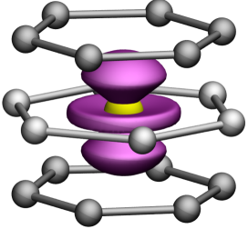
Figure 1: Schematic of the RECo₅ crystal structure, showing the RE (yellow) and Co sites (gray). The 2$c$ sites (referred to as Co_I in the text) are in-plane with the RE, and the 3$g$ sites (Co_II) lie above and below. An isosurface plot representing the Sm-4$f$ charge density, obtained as the sum of the squared spherical harmonics with $l=3,m=3,2,...,-1$ is also shown.

In this work we introduce a theory which attacks these two problems directly. Finite temperature effects are modeled within the disordered local moment (DLM) Györffy et al. (1985); Staunton et al. (2006) picture, which is reviewed in Section II. Meanwhile the problematic RE-$4f$ electrons are treated within DFT using the local self-interaction correction (LSIC) Lüders et al. (2005). Previous modeling of REs within this framework has been limited to Gd Mendive-Tapia and Staunton (2017); Patrick et al. (2017); Petit et al. (2015); Hughes et al. (2007), but the developments described in Section III now allow investigation of the entire RE series for the same computational cost. We use the new theory to study the RECo₅ family of magnets (Fig. 1), exploring the evolution of magnetism from 0 K (Sec. IV) to $T_{\mathrm{C}}$ (Sec. V). We conclude with our analysis of why, as is observed experimentally, the calculations find SmCo₅ to have the highest $T_{\mathrm{C}}$ of the RECo₅ magnets (Sec. VI).

II The DFT-DLM approach

At finite temperature, the functional properties of all materials are modified to some extent due to the thermal population of excited vibrational states, e.g. thermal expansion or increased electrical resistivity Baroni et al. (2001); Giustino (2017). However, independent of lattice vibrations, the magnetic properties of a material are extremely sensitive to temperature. The disordered local moment (DLM) picture of magnetism provides a conceptual basis to understand this temperature variation Györffy et al. (1985). Here the material is modeled as an array of microscopic magnetic moments (e.g. one associated with each atom), of fixed magnitude but variable orientation. This picture of local moments makes no assumption that the electrons themselves are localized; for example, the 3$d$ electrons responsible for magnetism in Fe, the prototypical DLM metal, are completely itinerant Staunton (1994). Rather, the spin-spin correlation between electrons near atomic sites can be strong enough to establish magnetically-polarized regions which exist for much longer timescales than those associated with electron motion Györffy et al. (1985). These are the local moments.

A DLM magnetic microstate is specified by the orientations $\{\bm{\hat{e}_{i}}\}=\{\bm{\hat{e}_{1}},...,\bm{\hat{e}_{N}}\}$ of the $N$ local moments. The grand potential energy $\Omega(\{\bm{\hat{e}_{i}}\})$ is a function of these local moment orientations, and the (classical) statistical mechanics of the system is determined by the partition function

$$Z=\int d\bm{\hat{e}_{1}}d\bm{\hat{e}_{2}}...d\bm{\hat{e}_{N}}\exp\left[-\beta\Omega(\{\bm{\hat{e}_{i}}\})\right],$$ (1)

where $1/\beta=k_{B}T$, and $T$ and $k_{B}$ are the temperature and Boltzmann constant. Experimental measurements correspond to thermal averages over the magnetic microstates. For instance, a magnetization measurement probes the average orientations of the local moments,

$$\langle\bm{\hat{e}_{j}}\rangle_{T}=\frac{1}{Z}\int\bm{\hat{e}_{j}}\ d\bm{\hat{e}_{1}}d\bm{\hat{e}_{2}}...d\bm{\hat{e}_{N}}\exp\left[-\beta\Omega(\{\bm{\hat{e}_{i}}\})\right].$$ (2)

The DLM paramagnetic state corresponds to each orientation averaging to zero, $\langle\bm{\hat{e}_{j}}\rangle_{T}=0$, and the highest temperature at which $\langle\bm{\hat{e}_{j}}\rangle_{T}\neq 0$ corresponds to the Curie temperature $T_{\mathrm{C}}$.

In principle, DFT provides a pathway to a first-principles DLM theory through the possibility of evaluating the grand potential energy $\Omega(\{\bm{\hat{e}_{i}}\})$, although finding a sufficiently accurate approximation for the exact exchange-correlation functional remains an ongoing and formidable challenge.Cohen et al. (2008); Illas et al. (2004) Specifically, $\Omega(\{\bm{\hat{e}_{i}}\})$ could be obtained from constrained DFT calculations, with the applied constraints forcing the local magnetizations to point along designated local moment directions $\{\bm{\hat{e}_{i}}\})$ Györffy et al. (1985). In practice however, any direct attempt to perform statistical mechanics would soon be faced with the problem of covering the huge phase space spanned by $\{\bm{\hat{e}_{i}}\}$, requiring an effectively infinite supercell to contain all $N$ local moments.

A popular method of circumventing this problem is to replace the “exact” $\Omega$ with a model, e.g. a Heisenberg model based on pairwise interactions between local moments. The model parameters are extracted from DFT calculations, e.g. from the Liechtenstein formula Liechtenstein et al. (1987) or constrained DFT Cao et al. (2009). $T_{\mathrm{C}}$ is then obtained from the simpler statistical mechanics of the model, which might be solved through a mean field approach, the random-phase approximation or Monte Carlo integration Rosengaard and Johansson (1997); Kashyap et al. (2003); Turek et al. (2003); Körmann et al. (2009); Fukazawa et al. (2017).

These schemes require striking a balance between a model which is sufficiently complex to capture the necessary magnetic interactions, yet simple enough for the statistical mechanics problem to be tractable. The most popular pairwise model should, as its name suggests, only apply when the interaction between two local moments is independent of the alignments of all other local moments in the system. This picture is not particularly intuitive in a metal where one would expect a co-operative effect, i.e. magnetic interactions being reinforced when the material is in a global ferromagnetic state and weakened in the paramagnetic state. Practically, this issue leads to the question of whether one should parametrize the pairwise model for the ferromagnetic or paramagnetic state Liechtenstein et al. (1987), and what to do at intermediate temperatures Körmann et al. (2014).

The DFT-DLM theory described in Györffy et al. (1985) approaches the problem in a different way. Instead of approximating the grand potential energy, one instead introduces an auxilliary quantity $\Omega_{0}(\{\bm{\hat{e}_{i}}\})$ with a known functional form,

$$\Omega_{0}(\{\bm{\hat{e}_{i}}\})=-\sum_{i}\bm{h_{i}}\cdot\bm{\hat{e}_{i}},$$ (3)

where the “Weiss fields” $\{\bm{h_{i}}\}$ are obtained self-consistently. Specifically, the thermodynamic inequality

$$F(T)\leq F_{0}(T)+\langle\Omega\rangle_{0,T}-\langle\Omega_{0}\rangle_{0,T}$$ (4)

provides a relation between the exact free energy $F(T)$ and the free energy of the auxiliary system, $F_{0}(T)=-k_{B}T\ln Z_{0}$, with

$$Z_{0}=\prod_{i}\int d\bm{\hat{e}_{i}}\exp[\bm{\lambda_{i}}\cdot\bm{\hat{e}_{i}}]=\prod_{i}\frac{4\pi}{\lambda_{i}}\sinh\lambda_{i}$$ (5)

and $\bm{\lambda_{i}}=\beta\bm{h_{i}}$. Crucially the thermal averages $\langle\rangle_{0,T}$ appearing in the inequality 4 are calculated with respect to the auxilliary system, e.g.

$$\langle\Omega\rangle_{0,T}=\frac{1}{Z_{0}}\prod_{j}\int d\bm{\hat{e}_{j}}\exp[\bm{\lambda_{j}}\cdot\bm{\hat{e}_{j}}]\Omega(\{\bm{\hat{e}_{i}}\}).$$ (6)

The Weiss fields are chosen to minimize the right hand side of the inequality 4. Then,

$$\bm{h_{i}}=-\frac{3}{4\pi}\int d\bm{\hat{e}_{i}}\langle\Omega\rangle_{0,T}^{\bm{\hat{e}_{i}}}\ \bm{\hat{e}_{i}}.$$ (7)

The partial average $\langle\Omega\rangle_{0,T}^{\bm{\hat{e}_{i}}}$ integrates over all the degrees of freedom in equation 6 except the single local moment orientation $\bm{\hat{e}_{i}}$. The Weiss fields have the periodicity of the magnetic unit cell, i.e. the number of distinct Weiss fields equals the number of magnetic sublattices.

As indicated by equation 7, the Weiss fields are temperature dependent. The DFT-DLM estimate of $T_{\mathrm{C}}$ is the temperature at which all the Weiss fields vanish. Alternatively, one can introduce local order parameters,

$$\bm{m_{i}}(T)\equiv\langle\bm{\hat{e}_{i}}\rangle_{0,T}=\bm{\hat{\lambda}_{i}}L(\lambda_{i})$$ (8)

with $L(\lambda_{i})=\coth(\lambda_{i})-1/\lambda_{i}$. These quantities vary between 1 at zero temperature and 0 at $T_{\mathrm{C}}$.

We stress that the key quantities in the DFT-DLM theory, the Weiss fields $\{\bm{h_{i}}\}$, are calculated with the full grand potential energy $\Omega$, without any assumption on the nature of the underlying interactions e.g. pairwise, four-spin etc Mendive-Tapia and Staunton (2017). Furthermore, through the averaging in equation 7 the magnitudes of the Weiss fields are indeed influenced by the degree of global order in the system, ensuring self consistency between $\{\bm{h_{i}}\}$ and the “reference state” used to calculate them.

The partial average $\langle\Omega\rangle_{0,T}^{\bm{\hat{e}_{i}}}$ appearing in equation 7 still presents a challenge to the most widely-used implementations of DFT, which solve the Kohn-Sham equations to determine single-particle wavefunctions Kohn and Sham (1965). However, the Green’s-function-based Korringa-Kohn-Rostoker multiple-scattering formulation of DFT, in combination with the coherent potential approximation (KKR-CPA) Györffy and Stocks (1979) allows the partial average to be recast as an impurity problem. This impurity problem, which sees each local moment sitting in an effective medium designed to mimic the averaged properties of the disordered system, can be solved using the same KKR-CPA techniques originally developed to tackle compositional disorder in the simulation of alloys Ebert et al. (2011). The DFT-DLM theory has undergone a number of developments from its original formulation, and is being applied to an increasingly wide range of magnetic systems Staunton et al. (2004); Hughes et al. (2007); Petit et al. (2015); Patrick et al. (2017, 2018).  The practical steps to calculating self-consistent Weiss fields and the key multiple-scattering equations are described in Refs. Patrick et al. (2017); Matsumoto et al. (2014); Staunton et al. (2006).

The fact that the DFT-DLM theory is rooted in KKR-CPA has both advantages and disadvantages. Thermally-averaged quantities, e.g. spin and orbital moments, can be calculated relatively easily by tracing the relevant operators with the Green’s function. The calculations include both core and valence electrons explicitly, and the structure of the KKR-CPA equations allow for a very high degree of numerical precision e.g. in evaluating integrals over the the Brillouin zone Bruno and Ginatempo (1997). However, the formalism generally involves making a shape approximation to the Kohn-Sham potential (here we use the atomic sphere approximation, ASA) which, although allowing a compact angular momentum basis to be used to describe the Green’s function and scattering matrices, is not expected to perform equally well for cubic and non-cubic crystal structures Andersen et al. (1991). In addition, we note that DFT-DLM is a mean-field theory, with the Weiss fields in equation 3 driving the magnetic ordering and vice versa. With these caveats in mind, we expect trends calculated across a series to be more robust than absolute values of specific quantities.

III Solving the Kohn-Sham-Dirac equation within the LSIC-LSDA

III.1 Relativistic DFT-DLM calculations

The large atomic number of the REs necessitates the use of relativistic (R) DFT-DLM theory to describe the spin-orbit coupling inherent in RE-TM magnets as well as mass-velocity and Darwin effects. Practically, our RDFT-DLM calculations involve two steps. In the first step, a self-consistent, scalar-relativistic DFT calculation is performed for a reference magnetic state. This reference magnetic state may be fully ordered (e.g. a ferromagnetic arrangement of spins) or fully disordered (the DLM/paramagnetic state). The output of this calculation is a set of atom-centered potentials. In the second step these potentials are fed into the fully-relativistic Kohn-Sham-Dirac (KSD) equation, thus treating spin-orbit coupling nonperturbatively. Combining the solutions of the KSD equation with the full KKR-CPA machinery allows the Weiss fields and $T_{\mathrm{C}}$ to be computed. Although not a methodological necessity Deák et al. (2014), the potentials here are kept “frozen” in the second step, i.e. the density derived from the Green’s function of the partially-ordered system is not used to update the potentials.

When constructing the potentials in the first step, in common with all DFT calculations it is necessary to make an approximation for the exchange-correlation energy. The local-spin-density approximation (LSDA) Kohn and Sham (1965); Vosko et al. (1980) performs rather well in describing the magnetism of itinerant electrons, but struggles to described the strongly-localized 4$f$ states which characterize REs Perdew and Zunger (1981). Furthermore, the orbital moments of transition metals are generally smaller than observed experimentally when calculated within the LSDA Eriksson et al. (1990). As a result, it is imperative to go beyond the LSDA exchange-correlation when modeling RE-TM magnets.

III.2 Treating RE-4$f$ electrons

Recent computational works performed at zero temperature have employed charge-self-consistent dynamical mean-field theory (DMFT) Kotliar et al. (2006), in particular using the Hubbard-$I$ approximation Lichtenstein and Katsnelson (1998), to calculate the magnetic moments of REs Locht et al. (2016) and RE-TM intermetallics like SmCo₅ Grånäs et al. (2012); Söderlind et al. (2017); Delange et al. (2017) and NdFe₁₂ Delange et al. (2017). The simpler, “open-core” scheme Brooks et al. (1991) constrains the total spin-density of the RE-4$f$ electrons to be that predicted by Hund’s rules Brooks et al. (1991); Richter and Eschrig (1991); Steinbeck et al. (2001); Söderlind et al. (2017); Fukazawa et al. (2017). Such calculations, which provide much important insight into RE-TM systems, bear some resemblance to crystal-field theory in the sense that the RE-4$f$ electrons are partitioned from the rest of the material, with the amount of hybridization they can undergo sensitive to how the calculation is set up Richter and Eschrig (1991); Delange et al. (2017). Alternative approaches like LDA/GGA+$U$ Larson et al. (2004, 2003); Waller et al. (2016), the orbital polarization correction (OPC) Söderlind et al. (2014) and the self-interaction correction (SIC) Lebègue et al. (2005) modify the potential at the RE site but treat all electrons equally, in principle allowing the RE-$4f$ states to hybridize freely Larson et al. (2004). An advantage of these schemes when studying trends across the RE-TM series is that, beyond initial choices about how the schemes are implemented, the calculations require minimal user input. Indeed the parameters entering the OPC and LDA/GGA+$U$ can be calculated from first-principles, e.g. the Racah parameters calculated from wavefunctions in the OPC Eriksson et al. (1990), or the $U$ and $J$ energies calculated from linear response Cococcioni and de Gironcoli (2005) or constrained random-phase approximation calculations Karlsson et al. (2010).

The SIC, which we employ here, aims to ensure that the exchange-correlation potential cancels the electrostatic (Hartree) energy of a single electron interacting with itself, which is not automatically realized in the LSDA Perdew and Zunger (1981). While the scheme becomes more complicated in extended systems, the localized nature of the RE-4$f$ electrons makes them particularly suitable for the SIC Lebègue et al. (2005). Furthermore, the SIC has already been formulated within the KKR-CPA theory as the local self-interaction correction (LSIC) Lüders et al. (2005). Indeed the LSIC has been previously used in DFT-DLM calculations to study Gd Mendive-Tapia and Staunton (2017); Patrick et al. (2017); Petit et al. (2015); Hughes et al. (2007); Patrick et al. (2018). However, in order to treat an arbitrary RE it is necessary to generalize the formalism. Conveniently, this same formalism allows the OPC to be also incorporated in the RDFT-DLM framework, facilitating an improved description of the Co orbital moments.

III.3 An LSIC-LSDA scheme based on Hund’s rules

The LSIC formalism Lüders et al. (2005) is based on applying the self-interaction correction to individual spin and orbital angular channels, each characterized by the pair of quantum numbers $\sigma L$. $\sigma$ labels spin, and $L$ is a composite quantum number which, in principle, labels a member of any complete set of angular momentum states. In the original LSIC implementation, these angular momentum states have the same symmetry as the nonmagnetic crystal Lüders et al. (2005). However, since the orbital moments are largely unquenched in the RE-TM compounds, here we choose $L$ to label the “atomic” $(l,m)$ quantum numbers associated with the complex spherical harmonics, i.e. eigenfunctions of the orbital angular momentum operator $\hat{l}_{z}$. As such, states that are degenerate in the nonmagnetic crystal may be split by the LSIC.

Figure 2: Scheme to correct RE-4$f$ states based on Hund’s rules. Each triangle corresponds to a single spin and orbital angular momentum channel i.e. $\sigma,l(=3),m$. LSIC channels with $\sigma=\uparrow$ ($\downarrow$) are represented by yellow (blue) triangles. We also show the moments obtained simply by adding the expectation values of the spin and orbital operators acting on the individual corrected states.

We must also choose which spin and orbital angular momentum channels we should apply the LSIC to. We propose to follow the scheme illustrated in Fig. 2, which is inspired by Hund’s rules. An extra LSIC channel is added for each RE-4$f$ electron, filling up $\sigma L$ combinations of the same spin ($\downarrow$) first with the largest available opposing $m$ (e.g. $m=+3$ for Ce). After entirely filling the $\downarrow$ channel at Gd, we start filling the $\uparrow$ channel, again starting with the largest available opposing $m$ (e.g. $m=-3$ for Tb) in accordance with the single-electron tendency of orbital and spin momenta to antialign Chikazumi (1997). As shown in Fig. 2, adding up the individual spin and orbital angular momentum contributions associated with these filled states gives quantities symmetric and antisymmetric respectively about Gd.

III.4 Including the LSIC/OPC in the KSD equation

The LSIC scalar-relativistic calculation (the first step referred to in Sec. III.1) proceeds as described in Ref. Lüders et al. (2005). At the second step in the RDFT-DLM procedure (and at variance with previous work Mendive-Tapia and Staunton (2017); Patrick et al. (2017); Petit et al. (2015); Hughes et al. (2007); Patrick et al. (2018)) the atom-centered potentials have a contribution which depends on angular momentum, conveniently written as

$$V_{\mathrm{SIC}}(\bm{r})=\sum_{L,\sigma}V_{L}^{\sigma}(r)\hat{P}_{L\sigma}.$$ (9)

Here $V^{\sigma}_{L}(r)$ is the spherically-symmetric correction to the potential obtained in the scalar-relativistic calculation Lüders et al. (2005), while $\hat{P}_{L\sigma}$ is a projection operator. In the Pauli representation these operators are $2\times 2$ matrices which are diagonal for spin polarization along the $z$ axis, whose elements project out states with angular momentum character $L$.

The angular-momentum dependent potentials result in a modified KSD equation,

$$\left[\bm{\tilde{\alpha}}\cdot\bm{p}c+\tilde{V}_{\mathrm{SIC}}+\tilde{I}(V(r)-W)\right.$$

$$\left.+\tilde{\beta}\left(\tilde{I}mc^{2}+\tilde{\sigma}_{z}B_{\mathrm{XC}}(r)\right)\right] \Psi=0.$$ (10)

Quantities with tildes are $4\times 4$ matrices; $\Psi$ is a bispinor, and $W$ and $m$ the electron energy and rest mass. Compared to the usual KSD equation Strange (1998), equation 10 has an extra term $\tilde{V}_{\mathrm{SIC}}$, simply related to $V_{\mathrm{SIC}}$ in equation 9:

$$\tilde{V}_{\mathrm{SIC}}=\begin{pmatrix}V_{\mathrm{SIC}}&0\\ 0&V_{\mathrm{SIC}}\end{pmatrix}.$$ (11)

We now follow the standard method of solving the radial KSD equation in multiple scattering theory Strange et al. (1984), i.e. we investigate the solutions

$$\Psi_{\nu}^{m_{j}}(\bm{r})=\sum_{\kappa_{1}}\begin{pmatrix}g^{m_{j}}_{\kappa_{1}\nu}(r)|\chi_{\kappa_{1}}^{m_{j}}\rangle\\ if^{m_{j}}_{\kappa_{1}\nu}(r)|\chi_{-\kappa_{1}}^{m_{j}}\rangle\ \end{pmatrix}.$$ (12)

The spin-angular functions $|\chi_{\kappa_{1}}^{m_{j}}\rangle$ are superpositions of the products of Pauli spinors and spherical harmonics weighted by Clebsch-Gordan coefficients Strange (1998). They are characterized by the quantum numbers $\kappa_{1}$ and $m_{j}$, and describe the angular character of free-particle solutions of the KSD equation. $\kappa_{1}$ is related to $j$, the sum of spin and orbital angular momentum in the spin-angular functions, with $\kappa=-l-1$ for $j=l+1/2$ and $\kappa^{\prime}=l$ for $j=l-1/2$. As indicated, we reserve the label $\kappa$ for negative values and $\kappa^{\prime}$ for positive values of $\kappa_{1}$. The label $\nu$ denotes the different solutions required to build the Green’s function in scattering theory, i.e. solutions with an asymptotic free-electron character which are regular or irregular at the origin Strange et al. (1984).

After inserting the trial solution 12 into equation 10 and performing a series of manipulations Strange (1998), we obtain coupled equations for the radial functions $f$ and $g$:

$$\frac{d{f^{m_{j}}_{\kappa\nu}}}{dr} = \frac{(\kappa-1)}{r}{f^{m_{j}}_{\kappa\nu}}+\frac{1}{\hbar c}(V-E){g^{m_{j}}_{\kappa\nu}}$$

$$+\frac{1}{\hbar c}\mathcal{G}^{m_{j}}_{+}(\kappa,\kappa){g^{m_{j}}_{\kappa\nu}}+\frac{1}{\hbar c}\mathcal{G}^{m_{j}}_{+}(\kappa,\kappa^{\prime}){g^{m_{j}}_{\kappa^{\prime}\nu}}$$

$$\frac{d{g^{m_{j}}_{\kappa\nu}}}{dr} = -\frac{(\kappa+1)}{r}{g^{m_{j}}_{\kappa\nu}}+\frac{1}{\hbar c}(E-V+2mc^{2}){f^{m_{j}}_{\kappa\nu}}$$ (13)

$$+\frac{1}{\hbar c}\mathcal{G}^{m_{j}}_{-}(-\kappa,-\kappa){f^{m_{j}}_{\kappa\nu}}.$$

Here, $E=W-mc^{2}$. The differential equations for $f^{m_{j}}_{\kappa^{\prime}\nu}$ and $g^{m_{j}}_{\kappa^{\prime}\nu}$ are obtained from equations 13 simply by interchanging $\kappa$ and $\kappa^{\prime}$. Crucially, compared to previous calculations which only included $B_{\mathrm{XC}}$, the basic structure of the coupled equations 13 is unchanged by the addition of $V_{\mathrm{SIC}}$. The difference is in the coupling functions,

$$\mathcal{G}^{m_{j}}_{\pm}(\kappa_{1},\kappa_{2})=\langle\chi_{\kappa_{1}}^{m_{j}}|(\sigma_{z}B_{\mathrm{XC}}\pm V_{\mathrm{SIC}})|\chi_{\kappa_{2}}^{m_{j}}\rangle.$$ (14)

$B_{\mathrm{XC}}(r)$ is now augmented by a linear combination of the LSIC potentials $V_{(l,m)\sigma}(r)$ weighted by Clebsch-Gordan coefficients. We give the explicit form of these coupling functions in the appendix A, but here just show an example of $\mathcal{G}^{m_{j}}_{\pm}(\kappa,\kappa)$ with $\kappa=-4$, $m_{j}=1/2$:

$$\mathcal{G}^{1/2}_{\pm}(-4,-4)=\frac{1}{7}B_{\mathrm{XC}}\pm\left[\frac{4}{7}V_{(3,0)}^{\uparrow}+\frac{3}{7}V_{(3,1)}^{\downarrow}\right].$$ (15)

We see that the coupling functions mix occupied, SI-corrected channels with unoccupied, non-SI-corrected channels, as discussed more in Appendix B.

It should be noted that, when deriving the coupled equations 13, additional coupling functions of the form $\mathcal{G}^{m_{j}}_{\pm}(-\kappa,\kappa+1)$ are introduced by both $\sigma_{z}$ and $V_{\mathrm{SIC}}$. Follow previous work Strange et al. (1984) we neglect these terms, which would otherwise result in an infinite ladder of couplings between orbital angular momenta $l$, $l\pm 2$, $l\pm 4$ etc. Ebert (2000).

The coupled equations 13, containing the appropriately weighted LSIC potentials, are solved numerically to give the scattering matrices and regular and irregular contributions to the Green’s function. From these quantities the entire RDFT-DLM computational machinery Matsumoto et al. (2014) can be applied without further modification.

The OPC enters the KSD equation in exactly the same way as the LSIC. This is most easily seen by writing the OPC analogy of equation 9 as Steinbeck et al. (2001); Ebert (2000)

$$V_{\mathrm{OPC}}(\bm{\hat{r}})=\sum_{l=2}\sum_{m,\sigma}-B_{l\sigma}m\langle\hat{l}_{z}\rangle_{\sigma}\hat{P}_{lm\sigma}.$$ (16)

where $B_{l\sigma}$ is a Racah parameter, and $\langle\hat{l}_{z}\rangle_{\sigma}$ is the spin-resolved expectation value for the relevant atom (we have anticipated applying the OPC to the $d$ channel). Thus the OPC can be considered a special case of the LSIC where the potential is independent of $r$, entering $\mathcal{G}^{m_{j}}_{\pm}(\kappa_{1},\kappa_{2})$ weighted by the coefficients in Appendix A. We stress that, since they only modify the coupling functions, the computational cost of including the LSIC or OPC is negligible.

III.5 Technical details

	$a$	$c$	$r_{\mathrm{ASA}}$	Ref.
YCo5	4.94	3.98	1.83/1.39/1.42	Andreev (1995)
LaCo5	5.11	3.97	1.91/1.40/1.44	Buschow (1977)
CeCo5	4.93	4.01	1.83/1.39/1.42	Andreev (1995)
PrCo5	5.01	3.99	1.86/1.40/1.43	Andreev (1995)
NdCo5	5.01	3.98	1.86/1.40/1.43	Andreev (1995)
SmCo5	4.97	3.98	1.85/1.39/1.42	Andreev (1995)
GdCo5	4.96	3.97	1.85/1.39/1.42	Andreev (1995)
TbCo5	4.94	3.97	1.84/1.39/1.42	Andreev (1995)
DyCo5	4.91	3.98	1.82/1.38/1.41	Andreev (1995)
HoCo5	4.91	3.97	1.82/1.38/1.41	Andreev (1995)
ErCo5	4.87	4.00	1.81/1.38/1.41	Buschow (1977)
TmCo5	4.86	4.02	1.81/1.38/1.41	Buschow (1977)

Table 1: Experimental lattice constants, taken from Refs. Andreev (1995); Buschow (1977). The ASA radii for the three non-equivalent sites (RE/Co_2c/Co_3g) are also given. All units are Å.

We generate the atomic-centered potentials in the fully-ordered (zero temperature) state in self-consistent scalar-relativistic LSIC-LSDA calculations Vosko et al. (1980); Lüders et al. (2005) within the ASA, as implemented in the hutsepot code Däne et al. (2009). Angular momentum expansions were truncated at $l_{\mathrm{max}}=3$, and the full Brillouin zone sampled on a 20$\times$20$\times$20 grid with state occupancies determined by a Fermi-Dirac distribution with an electronic temperature of 400 K. The calculations were performed using experimental lattice constants Andreev (1995); Buschow (1977), which are listed in Table 1 together with the ASA radii for the three nonequivalent sites in the RECo₅ structure. We used the same relations between ASA radii as in our previous work on YCo₅ and GdCo₅ Patrick et al. (2017).

For the RDFT-DLM calculations, apart from the inclusion of the LSIC described above we used the same computational setup (angular mesh, energy contour, electronic temperature) as in Patrick et al. (2017), including an adaptive sampling of the Brillouin zone Bruno and Ginatempo (1997). We applied the LSIC to the RE-$4f$ electrons and the OPC to the Co-$3d$ electrons. The magnitude of the OPC was determined iteratively at 0 K with the magnetization aligned along the $c$ axis, updating $\langle\hat{l}_{z}\rangle_{\sigma}$ at each iteration to self-consistency. The Racah parameters were calculated scalar-relativistically. The same OPC was used for all temperatures, consistent with the frozen-potential approach.

IV Zero-temperature calculations

IV.1 RECo₅ moments

We first use the RDFT-DLM formalism to calculate the magnetic moments of the RECo₅ series at zero temperature. To illustrate the trend across the lanthanide block we consider all members of the RE=Y–Lu series, including the non-forming RE = Pm, Eu, Yb and Lu compounds. Here, we fix the lattice parameters to those of GdCo₅; using the appropriate experimental RECo₅ lattice parameters (where available) produces very similar zero-temperature moments (Appendix C). For Ce, Pr and Nd we also performed calculations without applying the LSIC (i.e. treating the f-electrons as itinerant).

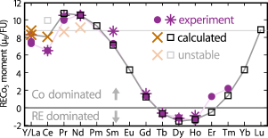
Figure 3: Magnetic moments calculated at zero temperature with (squares) and without (crosses) the LSIC applied, compared to experimental values reported in Refs. Buschow (1977) (circles) and Andreev (1995) (stars). Faint symbols were calculated to be energetically unfavorable. The gray horizontal line at 8.78$\mu_{\mathrm{B}}$ corresponds to the calculated YCo₅ moment.

In Fig. 3 we show the calculated RECo₅ moments and compare them to low-temperature experiments Buschow (1977); Andreev (1995). Here the Co moments are aligned along the $c$-axis, which defines the positive direction. A negative moment in Fig. 3 therefore means that the RE contribution to the magnetization is larger than that from the Co moments and is pointing in the opposite direction (RE-dominated). Usually, experimental measurements (e.g. on powdered samples) only measure the absolute magnetization. However, as we show below, RECo₅ compounds which are RE-dominated at 0 K show a compensation point (minimum) in their magnetization versus temperature curves, and Ref. Buschow (1977) reports compensation temperatures for Tb, Dy and HoCo₅. Accordingly we plot the experimental moments of these three compounds with minus signs.

Considering the calculations without the LSIC first (crosses in Fig. 3) we see relatively small variation for different REs, with the moments fluctuating around the YCo₅ value (shown as the gray horizontal line). We do observe a reduction in moment on moving from YCo₅ to LaCo₅, despite both elements having an empty 4$f$ shell. In fact, the moment of YCo₅ is much closer to that of LuCo₅, whose 4$f$ shell is totally filled. This behavior echoes that of quantities like melting points, electronegativities and ionization energies, which follow more naturally a Sc-Y-Lu series compared to Sc-Y-La Jensen (2015).

Applying the LSIC (squares in Fig. 3) has a dramatic effect on the magnetization, for instance increasing the moment of CeCo₅ by 2 $\mu_{\mathrm{B}}$/formula unit (FU). Now a strong variation with RE is observed, with PrCo₅/DyCo₅ achieving the largest TM/RE-dominated moments respectively. The transition from TM to RE-dominated magnetization occurs between Gd and Tb, and back to TM-dominated between Er and Tm.

In order to decide whether the calculations with or without the LSIC should be used to describe a given RE, we examine the total energies calculated at the scalar-relativistic level omitting spin-orbit coupling effects. This approach follows e.g. Refs. Lüders et al. (2005) and Strange et al. (1999), where the comparison of SIC total energies was used to determine the volume triggering the $\alpha\rightarrow\gamma$ transition in Ce or the valency of the rare earths and their sulphides. We find that applying the LSIC to PrCo₅ and NdCo₅ lowers the total energy, i.e. it is energetically favorable. Indeed for heavier REs the non-LSIC calculations become difficult to converge. However, applying the LSIC to CeCo₅ increases the scalar-relativistic total energy, indicating that the single Ce-4$f$ electron would prefer to be delocalized in this compound. Using this total energy as our criterion, we do not apply the LSIC to CeCo₅. Indeed the picture of the itinerant Ce-4$f$ electron has already been established in previous theoretical work Nordström et al. (1990). Other non-energetically-favorable calculations are shown in Fig. 3 as faint symbols.

The variation in RECo₅ moment calculated with the LSIC largely follows the simple picture presented in Fig. 2. In general the antiferromagnetic RE-TM exchange interaction causes the RE spin moments to point in the opposite direction to the Co moments Brooks et al. (1989), but whether or not the total RE moment aligns parallel or antiparallel depends on the sign and magnitude of the orbital contribution Nesbitt et al. (1962). The lightest REs have large orbital components pointing opposite to their spin which leads to parallel alignment of the total moments, whereas the spin and orbital moments of the heavy REs always reinforce each other to give antiparallel alignment.

IV.2 Decomposition of RECo₅ moments

	RE moment	Scalar rel.	Co moment	Total moment/FU	Exp. Buschow (1977)	Exp. Andreev (1995)
	(spin/orbital/total)	spin ($f$/$spd$)	(spin/orbital/total)
YCo5	-0.31/0.04/-0.28	-0.31 (0.00/-0.31)	7.54/1.25/8.78	8.50	7.52	8.3
LaCo5	-0.30/0.04/-0.26	-0.30 (-0.04/-0.25)	7.11/1.19/8.30	8.04	7.3	—
CeCo5	-0.92/0.51/-0.41	-0.86 (-0.57/-0.29)	7.07/1.40/8.47	8.06	6.5	6.5
CeCo5*	-1.37/2.97/1.60	-1.37 (-1.07/-0.30)	7.19/1.14/8.33	9.93	6.5	6.5
PrCo5	-2.46/4.88/2.42	-2.47 (-2.13/-0.34)	7.25/1.06/8.31	10.73	9.95	10.5
NdCo5	-3.56/5.74/2.18	-3.58 (-3.22/-0.37)	7.33/1.02/8.35	10.53	10.6	10.5
PmCo5	-4.63/5.60/0.97	-4.71 (-4.32/-0.39)	7.38/0.97/8.35	9.32	—	—
SmCo5	-5.63/4.55/-1.08	-5.82 (-5.41/-0.40)	7.36/0.85/8.21	7.13	7.3	8.7
EuCo5	-6.60/2.60/-4.01	-6.90 (-6.48/-0.42)	7.36/0.95/8.32	4.31	—	—
GdCo5	-7.50/0.03/-7.47	-7.49 (-7.00/-0.49)	7.43/1.27/8.70	1.23	1.37	1.6
TbCo5	-6.42/-2.96/-9.38	-6.41 (-5.98/-0.44)	7.44/1.28/8.72	-0.67	-0.68	-0.6
DyCo5	-5.33/-4.93/-10.26	-5.32 (-4.93/-0.39)	7.46/1.28/8.75	-1.52	-1.1	-1.2
HoCo5	-4.26/-5.88/-10.14	-4.20 (-3.86/-0.34)	7.51/1.29/8.80	-1.34	-1.49	-0.9
ErCo5	-3.28/-5.89/-9.17	-3.09 (-2.78/-0.31)	7.40/1.27/8.67	-0.50	1.28	—
TmCo5	-2.27/-4.92/-7.19	-2.00 (-1.71/-0.29)	7.32/1.25/8.57	1.38	2.2	—
YbCo5	-1.26/-2.95/-4.22	-0.92 (-0.65/-0.27)	7.30/1.24/8.53	4.32	—	—
LuCo5	-0.29/0.04/-0.25	-0.30 (-0.03/-0.27)	7.59/1.29/8.88	8.63	—	—

Table 2: Decomposition of zero-temperature moments. All quantities are in $\mu_{\mathrm{B}}$. For comparison we include the calculations for CeCo₅ with the LSIC applied (*) even though it is energetically unfavorable.

In Table 2 we resolve the calculated moments into spin and orbital contributions from the RE and TM. We also give the spin moments calculated at the scalar-relativistic level, which are further resolved into contributions of different angular momentum ($f$ or $spd$) character.

Concentrating first on the RE contribution to the magnetization, we see that the spin moments roughly track the expected spin of the LSIC channels, peaking at Gd. The scalar-relativistic decomposition shows the spin moments have an $spd$ component which increases from 0.25$\mu_{\mathrm{B}}$ for La to 0.49$\mu_{\mathrm{B}}$ for Gd. However, the $f$ components of the spin moment are not simply integers. Based on the simple picture of Fig. 2 this observation is surprising, since we would expect each localized RE-$4f$ electron to contribute $\pm$1$\mu_{\mathrm{B}}$ to the magnetization. Instead, we see that for each additional LSIC channel the change in $f$ components is closer to $\pm$1.1$\mu_{\mathrm{B}}$, until the elements with filled spin subshells (GdCo₅ and LuCo₅) are reached. This behavior indicates that the nominally unoccupied RE-4$f$ states, which do not have the LSIC applied, are affecting the calculated properties.

The RE orbital moments also follow the general trend of Fig. 2, but are better described by $\mu_{o}=(2-g_{J})J$, where $g_{J}$ is the Landé factor Richter (1998). This textbook expression is obtained by projecting the orbital moment onto the total angular momentum direction, which is valid for strong spin-orbit coupling. It is therefore natural to ask whether the spin RE moments should in fact be described by $\mu_{s}=2(g_{J}-1)J$, which is the corresponding projection for spin Richter (1998). However, in our calculations the principal interaction affecting the spin moments is the scalar-relativistic exchange, which can be confirmed by noting the close agreement between the RDFT-DLM and scalar-relativistic spin moments in Table 2. Therefore, the spin-orbit interaction plays a relatively minor role in determining the spin moment and the considerations leading to $\mu_{s}$ do not apply. We note that this situation is qualitatively different to the open-core scheme Brooks et al. (1991), which fixes the RE spin moments to $\mu_{s}$.

Now considering the TM contribution to the magnetization, the most striking feature in Table 2 is the different behavior of the light and heavy RECo₅ compounds. The Co moments exhibit relatively small variations for the heavy REs except for LuCo₅ which, as already noted, behaves similarly to YCo₅. However the variations for the light REs are much larger. Moving from La to Eu, the Co spin and orbital moments increase and decrease respectively, and in general the total Co moments are smaller than for the heavy RECo₅ compounds. As we discuss in Sec. V, a qualitative difference in light and heavy RECo₅ behavior is also observed in $T_{\mathrm{C}}$.

IV.3 Comparison to experiment

When comparing to experiment, it is important to note that there is a sizeable scatter in the published data. We have taken experimental low-temperature moments from the review articles of Refs. Buschow (1977) and Andreev (1995) which agree reasonably well with each other except for YCo₅ and SmCo₅, which deviate by approximately 1$\mu_{\mathrm{B}}$. Also, we note that the RE = Tb–Tm compounds do not form with exact RECo₅ stoichiometry. Instead, due to defects where the RE is substituted with pairs (dumbbells) of Co atoms Kumar (1988), the compounds become increasingly Co-rich. For example, the actual stoichiometry of the RE=Tm compound reported in Ref. Buschow (1977) is TmCo₆.

With these limitations in mind, the calculations compare reasonably well to experiment in Fig. 3. Certainly a number of qualitative features are reproduced, e.g. a drop in moment from Y to La, a large increase from Ce to Pr, and RE-dominated magnetization for Tb–Ho.

For the special case of CeCo₅, we note that the energetically-unstable LSIC calculation gives a moment which is in qualitative disagreement with the experimental trend. Interestingly however, whilst the LSDA+OPC calculations are closer to experiment they still overestimate the CeCo₅ moment. Not including the OPC on the Co atoms rather improves the agreement (Ref. Nordström et al. (1990) and Appendix C), suggesting that, (like for the LSIC), there might be a criterion based on energetics to decide whether or not the OPC should be applied.

Apart from the cases of ErCo₅ and TmCo₅ where the experiments are Co-rich, the remaining compound where the discrepancy between calculations and experiment is quite large is SmCo₅, specifically compared to the value of 8.7$\mu_{\mathrm{B}}$/FU in Ref. Andreev (1995). Interestingly, a recent neutron diffraction experiment reported even larger local moments in SmCo₅, which add up to give a resultant magnetization in excess of 12$\mu_{\mathrm{B}}$/FU Kohlmann et al. (2018). Studies employing DMFT and open-core calculations have reported smaller Sm total moments of approximately -0.3$\mu_{\mathrm{B}}$, which would bring the total SmCo₅ moment closer to 8$\mu_{\mathrm{B}}$/FU Grånäs et al. (2012); Söderlind et al. (2017); Delange et al. (2017). Earlier GGA+$U$ calculations found a much larger total moment of 9.9$\mu_{\mathrm{B}}$/FU due to a ferromagnetic alignment of Sm and Co spins. The scatter in theoretical and experimental data hints at the richness of the physics of SmCo₅ which, as we show next, is also seen in $T_{\mathrm{C}}$.

V Finite-temperature calculations

V.1 Magnetization vs. temperature curves

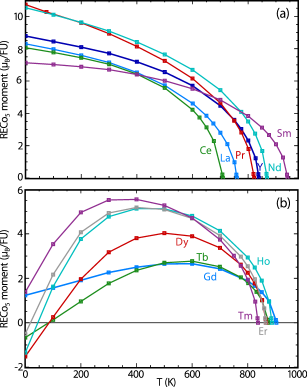
Figure 4: Magnetization per formula unit calculated at different temperatures for the (a) light and (b) heavy RECo₅ compounds. Calculations were performed at the GdCo₅ lattice parameters.

We now include local moment disorder within the RDFT-DLM picture. Figures 4(a) and (b) show the magnetization versus temperature ($M$v$T$) curves calculated for light and heavy RECo₅ compounds. These calculations were performed at the GdCo₅ lattice constants (Table 1). The light REs show behaviour associated with ferromagnets, i.e. a monotonic decrease in magnetization with increasing temperature. By contrast the heavy RECo₅ compounds have magnetizations which initially become more positive (TM-dominated) as the temperature increases, before reducing at higher temperatures. As we have shown previously by comparing YCo₅ and GdCo₅ Patrick et al. (2017) this contrasting behaviour is due to the RE moments disordering more quickly with temperature compared to the antiferromagnetically-aligned Co sublattice. As a result, the strong negative contribution to the total magnetization from the heavy RE diminishes quickly, leaving the positive Co magnetization.

In the case that the zero-temperature magnetization is RE-dominated, there is a compensation temperature at which the strongly-disordered RE magnetization cancels the weakly-disordered Co magnetization. Our calculated compensation temperatures are 84 K (TbCo₅), 85 K (DyCo₅), 45 K (HoCo₅) and 19 K (ErCo₅). Ref. Buschow (1977) reports experimental compensation temperatures of 110 K (TbCo₅), 123 K (DyCo₅) and 71 K (HoCo₅).

We note that the calculated $M$v$T$ curves have finite slopes at $T=0$ K, while experimentally-measured curves tend to be flat Patrick et al. (2017). The origin of this discrepancy is the classical statistical mechanics used in the DLM picture (equation 3), which does not give an energy barrier between the zero-temperature arrangement of local moments and an excited state where the moments have undergone infinitesimal rotations.

V.2 RE order parameters

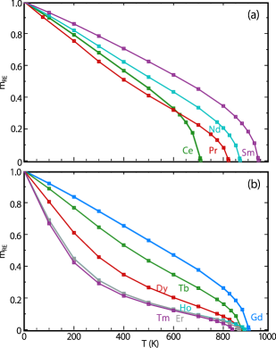
Figure 5: RE order parameters $m_{\mathrm{RE}}$ (equation 8) from the calculations of Fig. 4 on the light (a) and heavy (b) RECo₅ compounds.

In order to analyse the RE contribution to the magnetization in more detail, in Figs. 5(a) and(b) we plot the temperature evolution of the RE order parameter $m_{\mathrm{RE}}$ (equation 8). The heaviest REs Ho, Er and Tm disorder very quickly with temperature, losing 50% of their ordering below 200 K. By contrast, the Sm sublattice retains its ordering to much higher temperatures, e.g. 50% ordering at 650 K. Although part of the reason for this behavior is the higher $T_{\mathrm{C}}$ of SmCo₅, plots of the order parameter against reduced temperature $T/T_{\mathrm{C}}$ (not shown) demonstrate that even when this factor is accounted for, Sm orders the most strongly.

Having an ordered RE at high temperature is useful for permanent magnets, since the magnetocrystalline anisotropy decays faster than $m_{\mathrm{RE}}$ Kuz’min and Tishin (2008). Therefore SmCo₅ has a double advantage of having a high magnetocrystalline anisotropy at low temperature, and a strong RE ordering to retain this anisotropy at high temperature.

V.3 Curie temperatures

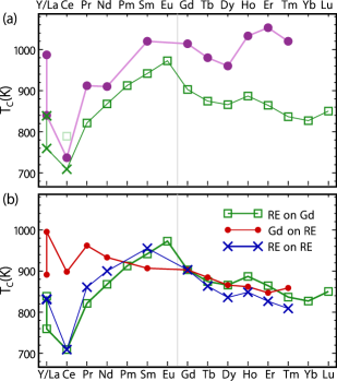
Figure 6: (a) $T_{\mathrm{C}}$ calculated for RECo₅ using the GdCo₅ lattice parameters, compared to the experimental values reported in Ref. Buschow (1977) (circles). Squares and crosses are calculated with and without the LSIC respectively, and the faint square is the energetically-unfavorable LSIC calculation for CeCo₅. (b) Comparison of $T_{\mathrm{C}}$ calculated for GdCo₅ using RECo₅ lattice parameters (circles), RECo₅ using GdCo₅ lattice parameters (squares), and RECo₅ using RECo₅ lattice parameters (crosses). The faint gray lines separate light and heavy REs.

In Fig. 6(a) we compare the calculated Curie temperatures $T_{\mathrm{C}}$ (extracted from Fig. 4) to the experimental values reported in Ref. Buschow (1977). We include $T_{\mathrm{C}}$ calculated for the non-forming Pm, Eu, Yb and LuCo₅ compounds. We remind the reader that experimental values are for Co-rich heavy RECo₅ compounds, for which we would expect an increased $T_{\mathrm{C}}$. For instance, the measured $T_{\mathrm{C}}$ of Gd₂Co₁₇ is 200 K higher than GdCo₅ Buschow (1977).

Fig. 6(a) clearly shows the contrasting behavior of the light and heavy RECo₅ compounds. Apart from YCo₅ and CeCo₅, the $T_{\mathrm{C}}$ of the light RECo₅ compounds increases monotonically with the number of RE-4$f$ electrons. Indeed, applying the energetically-unfavorable LSIC to the Ce-4$f$ electron also causes CeCo₅ to follow this trend [faint square in Fig. 6(a)]. Of the experimentally-known RECo₅ compounds, SmCo₅ is calculated to have the highest $T_{\mathrm{C}}$ (942 K), but the $T_{\mathrm{C}}$ of the non-forming EuCo₅ compound is found to be even higher, at 973 K.

The trend in calculated $T_{\mathrm{C}}$ of the heavy RECo₅ compounds is less obvious. In general, filling the remaining subshell causes a reduction in $T_{\mathrm{C}}$, but a secondary peak is observed at HoCo₅. This peak in $T_{\mathrm{C}}$ coincides with a slight peak in Co moments for HoCo₅ at zero temperature (Table. 2). Also, the $T_{\mathrm{C}}$ of LuCo₅ is very close to that calculated for YCo₅ (850 and 839 K respectively).

The calculations and experiments agree on a number of qualititative features. First, there is a substantial drop in $T_{\mathrm{C}}$ on moving from YCo₅ to LaCo₅, and another from LaCo₅ to CeCo₅. As already noted, the drop for CeCo₅ is not observed if the Ce-$4f$ electron is localized with the LSIC. Second, SmCo₅ has the highest $T_{\mathrm{C}}$ of all the experimentally-attainable RECo₅ compounds. Finally, the Co-rich heavy RECo₅ compounds do show a secondary peak in $T_{\mathrm{C}}$ like the calculations, although at Er not Ho. The heavy RE₂Co₁₇ compounds, whose stoichiometry is better defined, also show a secondary peak around Ho/Er/Tm followed by a sharp upturn for Lu Buschow (1977).

The calculated variation in $T_{\mathrm{C}}$ shown in Fig. 6(a) is only due to changing the RE. In order to quantify the magnetostructural effect of varying the lattice, we also calculated $T_{\mathrm{C}}$ for the RECo₅ compounds using experimentally-reported lattice parameters (Table 1). We further performed calculations where we varied the lattice but fixed the RE to Gd, i.e. GdCo₅ on different RECo₅ lattices. We compare the three different sets of calculations in Fig. 6(b).

First considering the calculations with the RE fixed to Gd [red circles in Fig. 6(b)], we observe a decrease in $T_{\mathrm{C}}$ across the lanthanide block. The exception is CeCo₅, which shows a strong magnetostructural effect; as shown in Table 1, CeCo₅ has an anomalously small $a$ parameter. These calculations do not reproduce experimental trends, e.g. predicting LaCo₅ to have the highest $T_{\mathrm{C}}$.

If instead we vary both the RE and the lattice parameters [blue crosses in Fig. 6(b)] we find the an almost identical trend in $T_{\mathrm{C}}$ as if we had kept the lattice parameters fixed at GdCo₅ (green squares). Using the RECo₅ lattice parameters accentuates the drop in $T_{\mathrm{C}}$ for CeCo₅. Unfortunately the experimentally-observed difference in $T_{\mathrm{C}}$ between YCo₅ and LaCo₅ is no longer calculated, which can be seen as a cancellation of competing green and red symbols in Fig. 6(b). In general, the calculations find magnetostructural effects to play a less important role in determining $T_{\mathrm{C}}$ than explicitly varying the RE.

V.4 Order parameter expansion of the free energy

Returning to the calculations with the lattice constants fixed to GdCo₅, to gain further insight into the calculated $T_{\mathrm{C}}$ we expand the RDFT-DLM potential energy $\langle\Omega\rangle_{0,T}$ in terms of the order parameters $m_{\mathrm{RE}}$, $m_{\mathrm{Co_{I}}}$ and $m_{\mathrm{Co_{II}}}$ Patrick et al. (2017). The labels I and II distinguish between the inequivalent Co positions in the RECo₅ structure (Fig. 1), i.e. the two Co atoms in plane with the RE (Co_I, Wyckoff position $2c$) and the three out-of-plane Co atoms (Co_II, Wyckoff position $3g$). In this expansion, the Weiss field at each site $(h_{\mathrm{RE}},h_{\mathrm{Co_{I}}},h_{\mathrm{Co_{II}}})$ is given by the equation

$$\begin{pmatrix}h_{\mathrm{RE}}\\ 2h_{\mathrm{Co_{I}}}\\ 3h_{\mathrm{Co_{II}}}\end{pmatrix}=\begin{pmatrix}J_{\mathrm{RE-RE}}&J_{\mathrm{RE-Co_{I}}}&J_{\mathrm{RE-Co_{II}}}\\ J_{\mathrm{RE-Co_{I}}}&J_{\mathrm{Co_{I}-Co_{I}}}&J_{\mathrm{Co_{I}-Co_{II}}}\\ J_{\mathrm{RE-Co_{II}}}&J_{\mathrm{Co_{I}-Co_{II}}}&J_{\mathrm{Co_{II}-Co_{II}}}\end{pmatrix}\begin{pmatrix}m_{\mathrm{RE}}\\ m_{\mathrm{Co_{I}}}\\ m_{\mathrm{Co_{II}}}\end{pmatrix}.$$ (17)

The prefactors in the Weiss fields account for the site multiplicities. The expansion of equation 17 is valid for small $m$, i.e. close to $T_{\mathrm{C}}$. The coefficients $J_{XY}$ are obtained by least-squares fitting of RDFT-DLM calculations. As discussed in Ref. Patrick et al. (2017), diagonalization of the matrix in equation 17 gives the RDFT-DLM $T_{\mathrm{C}}$, thus allowing the variation shown in Fig. 6(a) to be understood in terms of the strength of the interactions between different magnetic sublattices.

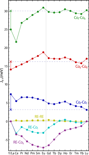
Figure 7: Different $J_{XY}$ parameters (c.f. equation 17) calculated for RECo₅ on the GdCo₅ lattice Note that the Ce calculation was performed without the LSIC, i.e. assuming that the Ce f-electron is itinerant. We highlight $J_{XY}$ for YCo₅ as crosses with horizontal dashed lines.

The calculated coefficients $J_{XY}$ are shown in Fig. 7. A negative $J_{XY}$ indicates a tendency for species $X$ and $Y$ to align antiferromagnetically. Comparing Figs. 6(a) and 7, we see that the behavior of $T_{\mathrm{C}}$ is mirrored by the largest $J_{XY}$ coefficient $J_{\mathrm{Co_{I}-Co_{II}}}$, which describes the inter-layer Co interaction. The next-largest coefficient $J_{\mathrm{Co_{II}-Co_{II}}}$, describing the intra-layer interactions of the pure Co layer, behaves similarly except that no drop at CeCo₅ is observed. It is not surprising either that $T_{\mathrm{C}}$ tracks the largest $J_{XY}$ coefficients or that these coefficients describe Co-Co interactions, in line with the picture that the TM is responsible for the high $T_{\mathrm{C}}$ in RE-TM magnets. What is less intuitive is that these coefficients should be so strongly affected by the RE.

As found for $T_{\mathrm{C}}$, there is clear distinction between light and heavy RECo₅ compounds for $J_{\mathrm{Co_{I}-Co_{II}}}$ and $J_{\mathrm{Co_{II}-Co_{II}}}$. By contrast $J_{\mathrm{Co_{I}-Co_{I}}}$ undergoes a general decrease from La–Lu, with slight fluctuations around Ho and a dip at Ce. The Co interactions are very similar for Y and Lu, consistent with their similar $T_{\mathrm{C}}$.

The $J_{\mathrm{RE}-Y}$ coefficients which quantify RE interactions are smaller in magnitude. $J_{\mathrm{RE}-\mathrm{RE}}$ is particularly weak and correlates with the size of the spin moment of the RE. The strongest RE-Co interactions are interplanar, RE-Co_II. Interestingly, neither $J_{\mathrm{Co_{II}-Co_{II}}}$ nor $J_{\mathrm{RE-Co_{II}}}$ show any strong anomaly at CeCo₅, indicating that it is only the Co_I interactions which are affected by the itinerant Ce-$4f$ electron.

Again comparing the light and heavy REs, we note that the in-plane interaction quantified by $J_{\mathrm{RE-Co_{I}}}$ actually becomes ferromagnetic for DyCo₅, HoCo₅ and ErCo₅, which coincides with the secondary peak in $T_{\mathrm{C}}$ [Fig. 6(a)]. Also, we observe that the strongest RE-Co interactions occur not for GdCo₅, which has the largest RE spin moment, but rather EuCo₅.

VI Discussion

VI.1 The RE-TM interaction

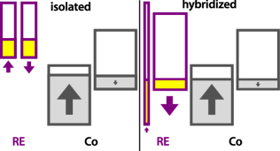
Figure 8: Schematic of antiferromagnetic RE-Co interaction, after Fig. 2 of Ref. Brooks et al. (1989). Wide/narrow rectangles symbolize strong/weak RE-Co hybridization in a given spin channel.

Our calculations have found that the strength of magnetic interactions between Co moments in RECo₅ is affected by the RE, even when the lattice parameters are held fixed. As a result of this variation, $T_{\mathrm{C}}$ depends heavily on the RE. To explain this behavior, we first recall the theory of RE-TM interactions described in Ref. Brooks et al. (1989), which explains the antiferromagnetic spin coupling in terms of hybridization between RE-5$d$ and TM-3$d$ states. Figure 8 is a schematic representation of the theory. The magnetic properties of Co originate from almost-full and almost-empty $3d$ bands of opposing spins. The minority spin Co-3$d$ band lies closer in energy to the RE-5$d$ bands than the majority Co-$d$ band, and therefore hybridizes more strongly. The preferential occupation of the lower-energy hybridized spin states causes the RE-5$d$ bands to develop a spin polarization in the direction of the Co minority spin, i.e. an antiferromagnetic coupling. Then, onsite RE 4$f$-5$d$ interactions polarize the RE-4$f$ spins in the same sense.

In this picture, the RE-TM interaction varies according to the strength of the 4$f$-5$d$ interaction, which is expected to scale with the spin moment of the RE. Accordingly, the strongest RE-TM interactions are expected for Gd. However, any effects on the TM magnetization are expected to proceed via the Co-3$d$-RE-5$d$ hybridization, with no direct link to the RE-$4f$ states.

VI.2 Magnetostructural effects

Within the picture of Fig. 8, any variation in $T_{\mathrm{C}}$ implies that the RE-5$d$ states are not the same for all REs. Of course, the RE-5$d$ orbitals do vary across the lanthanide block in terms of their spatial extent, as can be seen from the experimental lattice parameters in Table 1. The lattice parameter $a$ of LaCo₅ is 3% larger than GdCo₅, while for YCo₅ the difference is less than 0.5%. The experimental lattice parameters of LuCo₅ are not known, but the ionic radius of Lu is much closer to Y than La Taylor and Darby (1972). Correspondingly, the $T_{\mathrm{C}}$ values calculated at GdCo₅ lattice parameters are much closer for YCo₅ and LuCo₅ (11 K) than YCo₅ and LaCo₅ (80 K).

So, independent of any arguments based on the RE-4$f$ states, the calculations on YCo₅, LaCo₅ and LuCo₅ suggest that the size of the RE-5$d$ orbitals affects the Co magnetism. Indeed we could have reached a similar conclusion from our calculations on GdCo₅ with variable lattice parameter. Using the lattice parameters of lighter (heavier) RECo₅ compounds for GdCo₅ corresponds to expansion (compression) of $a$ (Table 1). From the red line of Fig. 6(b), we see that expansion of $a$ is correlated with an increased $T_{\mathrm{C}}$, while compression reduces it. Inversely, using GdCo₅ lattice parameters for the light and heavy RECo₅ compounds corresponds to compression and expansion of $a$ respectively. Comparing the green and blue symbols in Fig. 6(b) confirms that compression reduces $T_{\mathrm{C}}$ (green lower than blue for La–Gd) while expansion increases $T_{\mathrm{C}}$ (green higher than blue for Gd–Tm).

This magnetostructural effect makes some contribution to the overall variation of $T_{\mathrm{C}}$. Interestingly, the coefficients in Fig. 7 which quantify the Co_I-Co_I interaction (blue symbols) resemble the behavior of $T_{\mathrm{C}}$ calculated for GdCo₅ with different lattice parameters [red symbols in Fig. 6(b)]. Taken together with the fact that these Co_I atoms sit in plane with the RE atoms (Fig. 1), we assert that the variation $J_{\mathrm{Co_{I}-Co_{I}}}$ is magnetostructural in origin, with the RE-5$d$ orbitals affecting the in-plane Co-3$d$ interactions.

However, magnetostructural effects cannot really explain the observed variation in $T_{\mathrm{C}}$. First, they do not account for the qualitative difference in behavior between light and heavy RECo₅ compounds. Second, the $J_{\mathrm{Co_{I}-Co_{I}}}$ coefficients which are sensitive to the structure do not play a major role in determining $T_{\mathrm{C}}$, compared to $J_{\mathrm{Co_{I}-Co_{II}}}$ and $J_{\mathrm{Co_{II}-Co_{II}}}$. For example, LaCo₅ has the largest $J_{\mathrm{Co_{I}-Co_{I}}}$ but the second lowest $T_{\mathrm{C}}$ [Fig. 6(a)]. Therefore, we look for an additional explanation.

VI.3 Densities-of-states

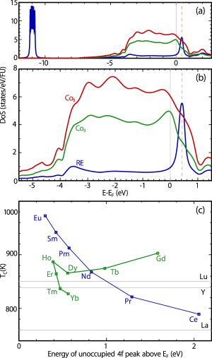
Figure 9: DoS calculated just below $T_{\mathrm{C}}$ for SmCo₅, resolved onto the Sm, Co_I and Co_II sublattices, shown (a) across a wide energy scale and (b) around the Fermi energy. The vertical dashed line intersects the center of the unoccupied 4$f$ peak above the Fermi energy. (c) $T_{\mathrm{C}}$ plotted against the center of this unoccupied peak for the different RECo₅ compounds. Note that here the value of $T_{\mathrm{C}}$ of CeCo₅ was calculated with the LSIC applied.

In Fig. 9(a) we plot the DFT Kohn-Sham density-of-states (DoS) of SmCo₅. The DoS was calculated just below $T_{\mathrm{C}}$ (i.e. at an almost completely disordered state), using GdCo₅ lattice parameters, and has been resolved into contributions from the RE, Co_I and Co_II sublattices. The wide energy scale of Fig. 9(a) was chosen to show explicitly the energy position of the occupied Sm-4$f$ states, 11 eV below the Fermi level $E_{F}$. Zooming in on the region around $E_{F}$ [Fig. 9(b)] shows the Co-$3d$ band (bandwidth $\sim$4 eV) hybridized with the RE-$5d$ states. However, an additional prominent feature is observed in the RE DoS, which is a narrow peak above $E_{F}$. The weight of this peak is approximately two electrons, and corresponds to the two unoccupied RE-$4f$ states in the $\downarrow$ spin channel (Fig. 2).

A similar peak can be observed in the DoS of all the RECo₅ compounds. For REs with almost empty 4$f$ spin subshells, the peak is located at high energy, and comes closer to $E_{F}$ as the subshell becomes filled (for light REs, a second peak corresponding to the opposite spin channel is also present, at much higher energies). We stress that in our DFT description, states above $E_{F}$ make no contribution to calculated properties. However, the tail of this unoccupied RE-4$f$ peak does extend below $E_{F}$ and therefore contributes to the density. In fact, this tail is the origin of the noninteger contribution to the $f$-resolved spin moments pointed out in Sec. IV.2 when discussing Table 2.

As indicated in Fig. 9(b), we can extract the energy corresponding to the centre of this unoccupied peak (dashed line). Then, in Fig. 9(c) we plot the calculated $T_{\mathrm{C}}$ as a function of this peak position. The light REs show an apparently strong correlation, with $T_{\mathrm{C}}$ increasing as the unoccupied peak becomes closer to $E_{F}$. By contrast the heavy REs do not show any particular correlation. The possible exception is HoCo₅, which as well as having a higher $T_{\mathrm{C}}$ than its neighbors also has the unoccupied RE-4$f$ peak closest to $E_{F}$.

An explanation for the differing behavior of the light and heavy RECo₅ compounds in Fig. 9(c) relates to the spin character of the unoccupied peak. For the light REs, the unoccupied RE-4$f$ peak closest to $E_{F}$ has the same $\downarrow$ spin as the Co-3$d$ minority spins, i.e. the states which hybridize strongly with the RE-5$d$ states and lead to antiferromagnetic coupling (Fig. 8). By contrast, the unoccupied RE-4$f$ peak of the heavy REs has the same $\uparrow$ spin character as the Co-$d$ majority spins. The hybridization of these states with RE-5$d$ is weak due to the energy separation; also, it favors ferromagnetic coupling. As noted when discussing Fig. 7, HoCo₅ does indeed have a positive $J_{\mathrm{RE}-\mathrm{Co_{I}}}$ coefficient, corresponding to a ferromagnetic RE-TM interaction. Indeed the temperature evolution of the order parameters in Fig. 5 shows how the overall antiferromagnetic RE-TM coupling is weakened for the heavy RECo₅ compounds.

We therefore propose a mechanism where a small contribution of $f$-character RE states, located just below the Fermi level, affects $T_{\mathrm{C}}$ by modifying the Co-3$d$ states, probably indirectly through the RE-5$d$ states. Such a mechanism could explain why we calculate higher $T_{\mathrm{C}}$s than GdCo₅ for Pm, Sm, and EuCo₅, despite these elements having smaller spin moments and being placed on a lattice with a compressed $a$ parameter. The effect is strong (weak) for the light (heavy) RECo₅ compounds, and favors antiferromagnetic (ferromagnetic) RE-TM coupling as described above, consistent with the behavior of $J_{\mathrm{RE}-\mathrm{Co_{I}}}$ and $J_{\mathrm{RE}-\mathrm{Co_{II}}}$ shown in Fig. 7.

We have already pointed out that the calculations have found SmCo₅ both to have the highest $T_{\mathrm{C}}$ of the experimentally-realized RECo₅ compounds and also a strong RE-TM interaction, which enables Sm to stay ordered at high temperature. Within the mechanism described here, the origin of this behavior is Sm’s almost-filled 4$f$ spin subshell. The hypothetical EuCo₅ compound would have an even higher $T_{\mathrm{C}}$, but unfortunately does not form. The total energies calculated at the scalar-relativistic level find Eu to be more stable in the 3+ state than 2+, when forced to occupy the RECo₅ structure. However, we have not investigated the full compositional phase diagram where different stoichiometries and structures might have a lower free energy.

VII Outlook

We have devised a physically transparent theory to model the magnetic properties of RE-TM compounds, with particular emphasis on their finite temperature properties. The magnetic disorder is described with the disordered local moment picture based on relativistic density-functional theory, with the RE-4$f$ electrons treated with the local self-interaction correction which encapsulates Hund’s rules. We used the theory to calculate the zero and finite temperature properties of the RECo₅ family of magnets, comparing magnetic moments and Curie temperatures to experimental measurements.

When presenting our theory we stated that, mainly as a result of the spherical approximations and mean-field nature of the theory, we expected our approach to perform best in calculating trends across a series. This statement has been borne out by our comparisons with experimental data, where we were able to reproduce a number of qualitative features. In particular we were able to track the behavior of $T_{\mathrm{C}}$, which to our knowledge has never been accomplished from first principles before.

We identified interesting behavior from the calculations, that even though $T_{\mathrm{C}}$ is generally determined by TM-TM interactions, these interactions were nonetheless affected by the RE. We argued that while the varying spatial extent of the RE-5$d$ orbitals did affect the TM-TM interactions, this effect was not sufficient to explain the variation in $T_{\mathrm{C}}$. Instead, we proposed a mechanism based on a small $f$-character contribution to the density around the Fermi level which, for the light RECo₅ compounds, strengthens both the RE-TM and TM-TM interactions.

We note that more expensive DMFT calculations do not provide an obvious pathway for a further exploration of this mechanism, neither in being able to calculate $T_{\mathrm{C}}$, nor also since we cannot make any assumptions about the hybridization of the RE-4$f$ electrons Delange et al. (2017). In terms of experimental evidence, we currently have only the observation that SmCo₅ has a higher $T_{\mathrm{C}}$ than GdCo₅. To our knowledge, this observation has not been explained before, but on its own cannot be considered justification for the correctness of the LSIC. However, the theory presented here opens the door to performing a more detailed comparision with experimental measurements on the temperature-dependent properties of any RE-TM compound, as was already done for YCo₅ and GdCo₅ Patrick et al. (2017).

Beyond exploring the fundamental physics of RE-TM magnets, our theoretical framework allows the study of practical aspects. In particular, the CPA formalism allows the effects of compositional disorder, e.g. substitution of RE or TM elements, to be investigated. Furthermore, with a view to optimizing high-temperature coercivity, it is highly desirable to tackle the temperature dependence of the magnetocrystalline anisotropy Staunton et al. (2004). Such calculations require a careful incorporation of crystal-field effects into our ASA calculations Hummler and Fähnle (1996) and also special care regarding how the calculated quantities are compared to experimental measurements, given the ferrimagnetic nature of the RE-TM magnets Patrick et al. (2018). Already the current calculations have found the high-temperature RE magnetic ordering to be strongest in SmCo₅, the best-performing magnet in the RECo₅ family.

Appendix A Coupling introduced by the LSIC

Here we list the formulae for the different coupling functions which enter the coupled equations 13. Again we emphasize that $\kappa=-l-1$ and $\kappa^{\prime}=l$. We have also introduced the quantities $\bar{l}_{1}=l+1$ and $\bar{l}_{2}=l-1$.

$$\mathcal{G}^{m_{j}}_{\pm}(\kappa,\kappa) = \frac{2m_{j}}{2l+1}B_{\mathrm{XC}}\pm\left[V_{l(m_{j}-1/2)}^{\uparrow}\left(\frac{l+m_{j}+1/2}{2l+1}\right)+V_{l(m_{j}+1/2)}^{\downarrow}\left(\frac{l-m_{j}+1/2}{2l+1}\right)\right]$$

$$\mathcal{G}^{m_{j}}_{\pm}(\kappa^{\prime},\kappa^{\prime}) = -\frac{2m_{j}}{2l+1}B_{\mathrm{XC}}\pm\left[V_{l(m_{j}-1/2)}^{\uparrow}\left(\frac{l-m_{j}+1/2}{2l+1}\right)+V_{l(m_{j}+1/2)}^{\downarrow}\left(\frac{l+m_{j}+1/2}{2l+1}\right)\right]$$

$$\mathcal{G}^{m_{j}}_{\pm}(\kappa,\kappa^{\prime}) = -\left(1-\frac{m_{j}^{2}}{(l+1/2)^{2}}\right)^{\frac{1}{2}}\left[B_{\mathrm{XC}}\mp\frac{V_{l(m_{j}-1/2)}^{\uparrow}-V_{l(m_{j}+1/2)}^{\downarrow}}{2}\right]=\mathcal{G}^{m_{j}}_{\pm}(\kappa^{\prime},\kappa)$$

$$\mathcal{G}^{m_{j}}_{\pm}(-\kappa,-\kappa) = -\frac{2m_{j}}{2\bar{l}_{1}+1}B_{\mathrm{XC}}\pm\left[V_{\bar{l}_{1}(m_{j}-1/2)}^{\uparrow}\left(\frac{\bar{l}_{1}-m_{j}+1/2}{2\bar{l}_{1}+1}\right)+V_{\bar{l}_{1}(m_{j}+1/2)}^{\downarrow}\left(\frac{\bar{l}_{1}+m_{j}+1/2}{2\bar{l}_{1}+1}\right)\right]$$

$$\mathcal{G}^{m_{j}}_{\pm}(-\kappa^{\prime},-\kappa^{\prime}) = -\frac{2m_{j}}{2\bar{l}_{2}+1}B_{\mathrm{XC}}\pm\left[V_{\bar{l}_{2}(m_{j}-1/2)}^{\uparrow}\left(\frac{\bar{l}_{2}-m_{j}+1/2}{2\bar{l}_{2}+1}\right)+V_{\bar{l}_{2}(m_{j}+1/2)}^{\downarrow}\left(\frac{\bar{l}_{2}+m_{j}+1/2}{2\bar{l}_{2}+1}\right)\right]$$

Appendix B Relativistic couplings between different spin-orbital channels

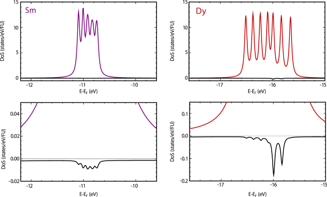
Figure 10: Spin-resolved, zero-temperature DoS for SmCo₅ (left) and DyCo₅ (right), at energies corresponding to the majority-spin, SI-corrected states. The majority and minority spin contributions are plotted with positive and negative signs, respectively, and the lower plots zoom in on the minority contribution. Note the larger scale for DyCo₅.

As indicated by equation 15, the spin-orbit interaction mixes different ($\sigma,m$) channels, including those which do and do not have the LSIC applied. In general, since there is a large energy separation between corrected and uncorrected states ($\sim$10 eV), the energy denominator that appears in the perturbative expansion of the state is large and thus the mixing is small. Nonetheless, the mixing can be seen by examining the zero-temperature, spin-resolved DoS at energies around the occupied (majority spin) 4$f$ electrons.

This quantity is plotted in Fig. 10 for SmCo₅ and DyCo₅. In the scalar-relativistic calculation the occupied 4$f$ electrons are spin pure, but on performing the relativistic calculation a small contribution appears in the minority spin channel (negative scale in Fig. 10), due to the mixing described above. This contribution is bigger for DyCo₅ than SmCo₅ (note change of scale) because there are two SI-corrected minority spin states located 4 eV above the majority spin peak which mix more strongly. For SmCo₅ the mixing only occurs with SI-uncorrected states lying above the Fermi level. The large energy separation suppresses the mixing in this case.

Appendix C Zero-temperature moments calculated at experimental lattice parameters

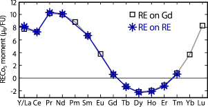
Figure 11: Magnetic moments calculated at zero temperature for RECo₅ using GdCo₅ lattice parameters (squares), and RECo₅ using RECo₅ lattice parameters (stars).

In Fig. 11 we compare the zero temperature moments calculated either using GdCo₅ lattice parameters or, where available, RECo₅ lattice parameters (Table 1). Note that these calculations were performed without the OPC applied, which results in reduced Co moments compared to Fig. 3.