Statistical Significance of CP Violation in Long Baseline Neutrino Experiments

Abstract

The p-value or statistical significance of a CP conservation null hypothesis test is determined from counting electron neutrino and antineutrino appearance oscillation events. The statistical estimates include cases with background events and different data sample sizes, graphical plots to interpret results and methods to combine p-values from different experiments. These estimates are useful for optimizing the search for CP violation with different amounts of neutrino and antineutrino beam running, comparing results from different experiments and for simple cross checks of more elaborate statistical estimates that use likelihood fitting of neutrino parameters.

1 Introduction

The search for charge-parity (CP) symmetry violation in neutrino interactions[1] is a major effort in the current[2] and future[3] particle physics program. A violation of this fundamental symmetry may be related to the matter-antimatter imbalance observed in the universe and testing this symmetry is now a fundamental physics question. This search can be performed using long baseline neutrino experiments by measuring the neutrino and antineutrino appearance oscillation probabilities, $P\left(\nu_{\mu}\rightarrow\nu_{e}\right)$ and $P\left(\overline{\nu}_{\mu}\rightarrow\overline{\nu}_{e}\right)$, respectively. The conservation of the CP symmetry predicts these probabilities are equal in vacuum,

$$P\left(\nu_{\mu}\rightarrow\nu_{e}\right)=P\left(\overline{\nu}_{\mu}\rightarrow\overline{\nu}_{e}\right)$$ (1)

These probability values depend[1] on neutrino mixing angles, mass splittings, CP phase and $E/L$, where $E$ is the neutrino or the antineutrino energy and $L$ is the oscillation distance between the neutrino origin and its measurement position. CP conservation (CPC) predicts while travelling in vacuum that the neutrino probability and the antineutrino probability are equal. If these probabilities are not equal, then there is CP violation (CPV) in the neutrino sector. In the case of neutrinos travelling in dense matter over very long distances, these probabilities can differ due to the MSW effect[4]. The purpose of this paper is to examine various p-value hypothesis tests of CP conservation (called the null hypothesis) in long baseline neutrino test measurements

The experimental setup typically has a proton beam striking a target which produces positive and negative mesons that are selectively focused into a long decay pipe to produce either predominately $\nu_{\mu}$ and $\overline{\nu}_{\mu}$ beams, that are measured in a near neutrino detector and which continue to travel a long baseline distance to be observed in a far neutrino detector. As the $\nu_{\mu}$ and $\overline{\nu}_{\mu}$ beams travel to the far detector a fraction may under go oscillations into $\nu_{e}$ and $\overline{\nu}_{e}$ events, respectively, which are detected in the far detector. The neutrino and antineutrino rates are determined by measurements of the following inclusive interactions,

$$\begin{array}[]{ccc}\nu_{\mu}+N&\rightarrow&\mu^{-}+X\\ \overline{\nu}_{\mu}+N&\rightarrow&\mu^{+}+X\\ \nu_{e}+N&\rightarrow&e^{-}+X\\ \overline{\nu}_{e}+N&\rightarrow&e^{+}+X\end{array}$$ (2)

The direct test of CP conservation uses four sample populations which are the observed numbers of the unoscillated $\nu_{\mu}$ and $\overline{\nu}_{\mu}$ events at the near detector and the $\nu_{e}$ and $\overline{\nu}_{e}$ appearance events at the far detector. The main statistical errors will come from the limited sample size of the appearance events. A simple test statistic[5] can be formed that is the difference of the two numbers of appearance events with an assumed known value of the CPC oscillation probabilities. Measurements of this difference can be used to calculate the p-value probability that a null hypothesis (CP conservation) could obtain at least this difference or more extreme values. In the next two sections simple examples are presented and then neutrino and antineutrino measurements are introduced. This is followed by sections describing specific neutrino cases.

2 Examples of null hypothesis tests using differences of two Poisson distributions

Several Poisson type test statististics[6] have been used extensively in other research areas for p-value calculations. An illustrative example is finding the probability that two soccer teams, that are rated to score the same goals per game, would have a game with a difference of $\Delta$ goals or larger. Suppose teams A and B are expected to both score on average 2.5 goals per game. A test statistic, called a Skellam distribution[5], of the difference in their scores forms a random integer variable that is the difference of two Poissons. The probability $P^{SK}$ as a function of the integer difference $\Delta$ is the convolution of the two Poissons with averages $\lambda_{A}=\lambda_{B}=2.5$,

$$P^{SK}\left(\Delta\right)=\sum_{n=-\infty}^{\infty}\frac{e^{-\lambda_{A}}\lambda_{A}^{\left(\varDelta+n\right)}}{\left(\varDelta+n\right)!}\frac{e^{-\lambda_{B}}\lambda_{B}^{n}}{n!}$$ (3)

The Skellam distribution is a 1-dimensional test statistic that is the probability $P^{SK}\left(\Delta\right)$ versus $\Delta=n_{A}-n_{B}$. This is plotted in Fig. 1 (a).

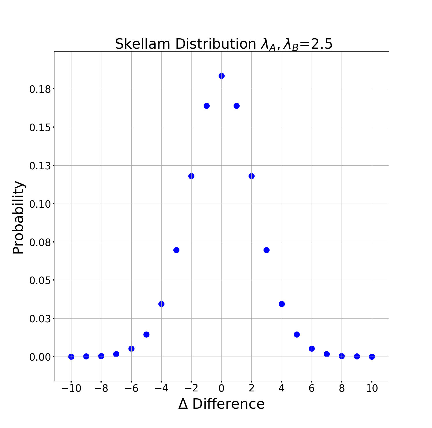
(a)

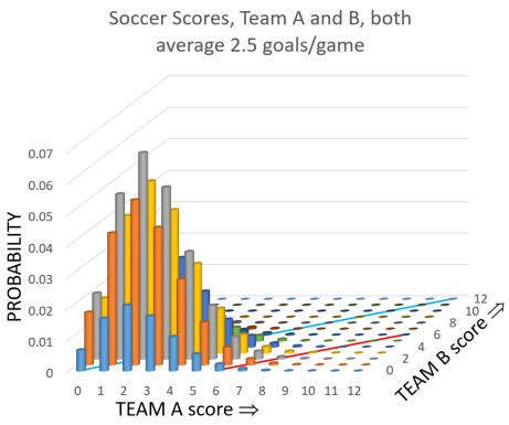
(b)

Fig. 1. The Skellam distribution, shown in (a), of the difference of scores between soccer team A and B assuming each team has an average of 2.5 goals per game. Note if team A and B has a difference of 6 goals, then this corresponds to a probability of 0.00534 and the difference of obtaining 6 or more goals is 0.00774 which is the sum of probabilities for $\Delta\geq 6$ . In (b) is the Poisson probability Lego plot of team A versus team B scores. The blue diagonal lines, $N_{A}=N_{B}$, corresponds to both teams getting the same score which is equivalent to the null hypothesis of team A and B having equal average scores. The red diagonal line corresponds to a difference boundary, $N_{A}=N_{B}+6$, with team A getting 6 goals more than team B. The sum of the probabilities of all scores on and to the right of the red line correspond to the p-value of a particular team A getting 6 or more goals than team B. Note that the diagonal lines are parallel with slope 1 and separated by 6 goals.

Suppose in a game, the teams had $N_{A}$=7 and $N_{B}$=1 goals. This particular game (or test measurement) with a difference of 6 goals has a probability of $P^{SK}\left(\Delta=6\right)=5.34\times 10^{-3}$. The probability of obtaining difference of 6 $or$ $more$ goals is,

$$\sum_{N_{A}=0}^{\infty}\sum_{N_{B}=0}^{\infty}\theta\left(N_{A}-N{}_{B}-\Delta+\epsilon\right)\frac{e^{-\lambda_{A}}\lambda_{A}^{N_{A}}}{N_{A}!}\frac{e^{-\lambda_{A}}\lambda_{B}^{N_{B}}}{N_{B}!}$$ (4)

which sums to $7.74\times 10^{-3}$ assuming $\lambda_{A}=\lambda_{B}=2.5$. This corresponds to the p-value which is the probability the null hypothesis, which assumes the same average $2.5$, can reach this extreme value or higher. The joint Poisson probabilities as a function of team A and B scores are displayed in Fig. 1(b). The blue diagonal line, $N_{A}=N{}_{B}$, corresponds to both teams having equal score probabilities. The red line, $N_{A}=N_{B}+6$, is the boundary, parallel to the blue line, that represents the difference of team A having six goals more than team B. Each bin of the Skellam distribution sums the probabilities in Fig. 1(b), in between two diagonal lines that are separated by a perpendicular distance of $1/\sqrt{2}$.

The test measurement p-value of the null hypothesis (both teams had the same average score 2.5 goals) is the probability that a difference of 6 or higher goals occurs and in this example the p-value is 0.0024. This corresponds to a 3 standard deviation test of the null hypothesis that the teams had the same average number of goals per game.

Another example is a test if two radioactive samples have the same decay rates. Suppose there are two samples of radioactive nuclei type A and B with initially $N_{A}$ and $N_{B}$ nuclei, respectively, which are equal. Then suppose there are measurements of $n_{A}$ and $n_{B}$ decays in a time t. The null hypothesis is if these two samples have the same decay rate $\varGamma$. This can be tested by calculating the p-value of the null hypothesis where $n_{A}=N_{A}\left(1-e^{-\Gamma t}\right)$ and $n_{B}=N_{B}\left(1-e^{-\Gamma t}\right)$. In this example, suppose a measurement of the samples yielded $n_{A}$ and $n_{B}$. The p-value that the radioactive samples are the same is calcuated with Eq. (6) where $\lambda_{A}=n_{A}$= $\lambda_{B}=n_{B}$ and $\Delta=n_{A}-n_{B}$.

3 Neutrino and Antineutrino Measurements

The test of CP violation in a long baseline neutrino experiment is analogous to testing if two radioactive nuclei samples have the same decay rates. The neutrino far detector counts the number of observed neutrino events $N_{e}$ found in a $\nu_{\mu}$ beam and the number of observed antineutrino events $\overline{N}_{e}$ found in a $\overline{\nu}_{\mu}$ beam and the difference is considered. The appearance probabilities in terms of observed events are,

$$P\left(\nu_{\mu}\rightarrow\nu_{e}\right)=\frac{N_{e}}{N_{\mu}}\text{ and }P\left(\overline{\nu}_{\mu}\rightarrow\overline{\nu}_{e}\right)=\frac{\overline{N}_{e}}{\overline{N}_{\mu}}$$ (5)

These number of events are averaged over $\left\langle E_{\nu}/L\right\rangle$ and $\left\langle E_{\overline{\nu}}/L\right\rangle$ where the neutrino and antineutrino energies should be identical. A test of the CPC hypothesis is performed by determining the p-value of the null hypothesis. Given experimental measurements of the $N_{e}$ and $\overline{N}_{e}$ and unoscillated $N_{\mu}$ and $\overline{N}_{\mu}$, the above probabilities can be obtained. The null hypothesis of CPC can also be formed using a test statistic such as the asymmetry $A$,

$$A=\frac{P\left(\nu_{\mu}\rightarrow\nu_{e}\right)-P\left(\overline{\nu}_{\mu}\rightarrow\overline{\nu}_{e}\right)}{P\left(\nu_{\mu}\rightarrow\nu_{e}\right)+P\left(\overline{\nu}_{\mu}\rightarrow\overline{\nu}_{e}\right)}$$ (6)

or the difference in the appearance rates, denoted as $\Delta$,

$$\Delta=N_{e}-\overline{N}_{e}$$ (7)

This assumes the unoscillated muon neutrino and antineutrino events samples at the far detector are the same, $N_{\mu}=\overline{N}_{\mu}$. This tests how unequal the probabilities are since,

$$P\left(\nu_{\mu}\rightarrow\nu_{e}\right)-P\left(\overline{\nu}_{\mu}\rightarrow\overline{\nu}_{e}\right)=\frac{N_{e}-\overline{N}_{e}}{N_{\mu}}$$ (8)

and it is seen that the p-value of a measurement difference test statistic $\Delta$ or more extreme is equivalent to measuring the corresponding neutrino-antineutrino probability difference in Eq. (6) or larger. If there are unequal sample sizes where $R=N_{\mu}/\overline{N}_{\mu}\neq 1$, then the above probability difference, $A$ and $\Delta$ become,

$$P\left(\nu_{\mu}\rightarrow\nu_{e}\right)-P\left(\overline{\nu}_{\mu}\rightarrow\overline{\nu}_{e}\right)=\frac{N_{e}}{N_{\mu}}-\frac{\overline{N}_{e}}{\overline{N}_{\mu}}=\frac{1}{N_{\mu}}\left(N_{e}-R\overline{N}_{e}\right)$$ (9)

$$A=\frac{N_{e}-R\overline{N}_{e}}{N_{e}+R\overline{N}_{e}}$$ (10)

$$\Delta=N_{e}-R\overline{N}_{e}$$ (11)

The $N_{e}$ and $\overline{N}_{e}$ are number of observed events averaged over neutrino energy. Again the p-value of the test statistic in Eq. (8) is equivalent to the p-value of the neutrino-antineutrino probability difference in Eq. (6). If the detector and the reconstruction efficiencies, the $\nu_{e}$ cross section, the $\overline{\nu}$_e cross section and the number of observed $N_{\mu}$ and $\overline{N}_{\mu}$ are included, the ratio $R$ becomes,

$$R=\left(\frac{\overline{\epsilon}_{e}}{\epsilon_{e}}\right)\frac{N_{\mu}/\epsilon_{\mu}}{\overline{N}_{\mu}/\overline{\epsilon}_{\mu}}$$ (12)

where $\epsilon_{e}$ and $\overline{\epsilon}_{e}$ are the efficiencies to reconstruct far detector events and $\epsilon_{\mu}$ and $\overline{\epsilon}_{\mu}$ are the efficiences to reconstruct the near detector events. Note a Poisson probability plotted as a function of $N_{e}$ versus $\overline{N}_{e}$, is analogous to Fig. 1(b), where the line representing equal rates, $0=N_{e}-R\overline{N}_{e}$, and the difference boundary $\Delta=N_{e}-R\overline{N}_{e}$ will be parallel to each other with slope $R$. The simple methods described here, should be useful to estimate p-value probabilities of the null CPV hypothesis. They require far detector measurements of the $N_{e}$ events in a neutrino beam, the $\overline{N}_{e}$ events in an antineutrino beam and the ratio of unoscillated rates of $\overline{N}_{\mu}/N_{\mu}$ at the far detector. If the long baseline experiment $E/L$, has muon neutrino disappearance that oscillates into zero events at the far detector, then a near detector will be essential to measure this ratio $\overline{N}_{\mu}/N_{\mu}$ and extrapolate the unoscillated rate ratio to the far detector. More complex methods to determine CPV include fitting the $E/L$ distributions to determine the Pontecorvo, Maki, Nakagawa and Sakata (PMNS) neutrino parameters[1], but due to the expected small statistics from neutrino long baseline neutrino experiments in the near term, the methods presented here should be adequate to predict p-value tests of CP violation. The difference test statistic $\Delta$ will not be affected by uncertainties of the PMNS neutrino parameters that include the mixing angles, CP phase and the mass hierarchy, however the magnitude of the probability depends on these PMNS parameters and this can affect the resulting p-value using a Skellam distribution. The aim in this paper is to test for CPV in Eqn. 1, independent of the values of the PMNS parameters.

In the following sections, different cases are presented with pedagogical examples. The material is presented in order of complexity and include cases; (I) equal data samples with no background, (II) equal data samples with background, (III) different data sample sizes, (IV) different sample sizes with backgrounds and (V), where the oscillation probabilies are assumed to be unknown. Finally a method to combine p-values from 2 different experiments is presented. Simple calculations and formulae are provided so the reader can replicate the results. In the appendix, the general case of an integrated flux measurement, cross sections, detection efficiencies and how their affects are included in the $R$ factor is described.

4 Case I. No Background and Equal Data Samples

The simplied case with no background and equal amounts of neutrino and antineutrino data is presented here. It is assumed, the reconstruction efficiency of the electron and muon neutrino interactions are the same and the uncertainties due to the numbers of $\nu_{\mu}$ and $\overline{\nu}_{\mu}$ are small compared to the uncertainties of the number of $\nu_{e}$ and $\overline{\nu}_{e}$ to simplify the equations. The simpliest test statistic is the difference in the number $\nu_{e}$ and $\overline{\nu}_{e}$ appearance events.

For our neutrino example, suppose at the far detector, the sample of the number of unoscillated muon neutrino and antineutrinos that could be reconstructed are the same,

$$N_{\mu}=\overline{N}_{\mu}$$ (13)

If CPC is true, the number of expected or average number of appearance events for neutrinos $\lambda$ and for antineutrinos $\overline{\lambda}$ should be equal.  The probability of a particular observation of $N_{e}$ and $\overline{N}_{e}$ will be,

$$\frac{e^{-\lambda}\lambda^{N_{e}}}{N_{e}!}\frac{e^{-\overline{\lambda}}\overline{\lambda}^{\overline{N}_{e}}}{\overline{N}_{e}!}$$ (14)

The Poisson probability is denoted as script $\mathscr{P}\left(N,\lambda\right)$ , where the double sum is always normalized,

$$\sum_{N_{e}=0}^{\infty}\sum_{\overline{N}_{e}=0}^{\infty}\mathscr{P}\left(N_{e},\lambda\right)\mathscr{P}\left(\overline{N}_{e},\overline{\lambda}\right)=\sum_{N_{e}=0}^{\infty}\mathscr{P}\left(N_{e},\lambda\right)\sum_{\overline{N}_{e}=0}^{\infty}\mathscr{P}\left(\overline{N}_{e},\overline{\lambda}\right)=1$$ (15)

The CPC p-value of observing a difference between the neutrino and antineutrino appearance rates, $N_{e}-\overline{N}_{e}\geq\Delta$ is given as

$$\sum_{N_{e}=0}^{\infty}\sum_{\overline{N}_{e}=0}^{\infty}\theta\left(N_{e}-\overline{N}_{e}-\Delta+\epsilon\right)\mathscr{P}\left(N_{e},\lambda\right)\mathscr{P}\left(\overline{N}_{e},\overline{\lambda}\right)$$ (16)

where $\theta\left(x\right)$ is the Heaviside or step function and where $1>\epsilon>0$ is added to ensure that the term where $N_{e}-\overline{N}_{e}=\Delta$ is counted. Note this can be rewritten in terms of modified Bessel function[5]. If a difference $\Delta$ is observed, the above formula is the extreme probability that the CPC hypothesis must have to produce a difference of $\Delta$ or larger.

Using the PMNS mixing matrix, the mixing angles and a nonzero CP phase, the CPV $\lambda$ and $\overline{\lambda}$ values and the resulting $\Delta$ can be determined and used to estimate the CPC p-value. Suppose for the CPC ($\delta_{CP}=0$) scenario these yield,

$$P\left(\nu_{\mu}\rightarrow\nu_{e}\right)=P\left(\overline{\nu}_{\mu}\rightarrow\overline{\nu}_{e}\right)=0.051$$ (17)

and for the CPV ($\delta_{CP}=-\pi/2$) scenario,

$$P\left(\nu_{\mu}\rightarrow\nu_{e}\right)=0.065$$ (18)

$$P\left(\overline{\nu}_{\mu}\rightarrow\overline{\nu}_{e}\right)=0.037$$ (19)

Then for sample size of $N_{\mu}=\overline{N}_{\mu}=1000,$ the predictions for CPC scenario, neutrino appearance in vacuum are,

$$N_{e}=\overline{N}_{e}=51$$ (20)

and for the CPV scenario the predictions are,

$$N_{e}=65$$ (21)

$$\overline{N}_{e}=37$$ (22)

The above CPV case predicts a difference value, $\Delta=65-37=28$ and with

$$\sum_{N_{e}=0}^{\infty}\sum_{\overline{N}_{e}=0}^{\infty}\theta\left(N_{e}-\overline{N}_{e}-28+\epsilon\right)\mathscr{P}\left(N_{e},65\right)\mathscr{P}\left(\overline{N}_{e},37\right)=0.59$$ (23)

This predicts there is a 59% chance of observing $\Delta$ with 28 or higher in a single measurement of the CPV scenario. The CPC case in vacuum has $\lambda$ and $\overline{\lambda}$ equal to 51 and the probability of a null CPC hypothesis is,

$$\sum_{N_{e}=0}^{\infty}\sum_{\overline{N}_{e}=0}^{\infty}\theta\left(N_{e}-\overline{N}_{e}-28+\epsilon\right)\mathscr{P}\left(N_{e},51\right)\mathscr{P}\left(\overline{N}_{e},51\right)=0.00242$$ (24)

Hence the p-value is 0.242% and the resulting double Poisson plot is given in the Fig. 2(a) with a boundary set by $\Delta=28$. The blue line in Fig. 2(a) is the boundary which is a 45^∘ line that lies on the boundary point at $N_{e}=65$ and $\overline{N}_{e}=37$. The Skellam distribution of the double Poisson distribution is plotted in Fig. 3(a). The arrow points to the 28 difference which corresponds to the 0.00242 probability which is the area to the left of the blue line. The p-value depends on the value of $\lambda$ and $\overline{\lambda}$. If $\lambda$ and $\overline{\lambda}$ were both equal to 46 or 56, then the resulting p-value (for the same $\Delta=28$) changes to 0.151 or 0.357, respectively. Note, if the mass effects are large, then unequal values of $\lambda$ and $\overline{\lambda}$ should be used for the null hypothesis.

(c)

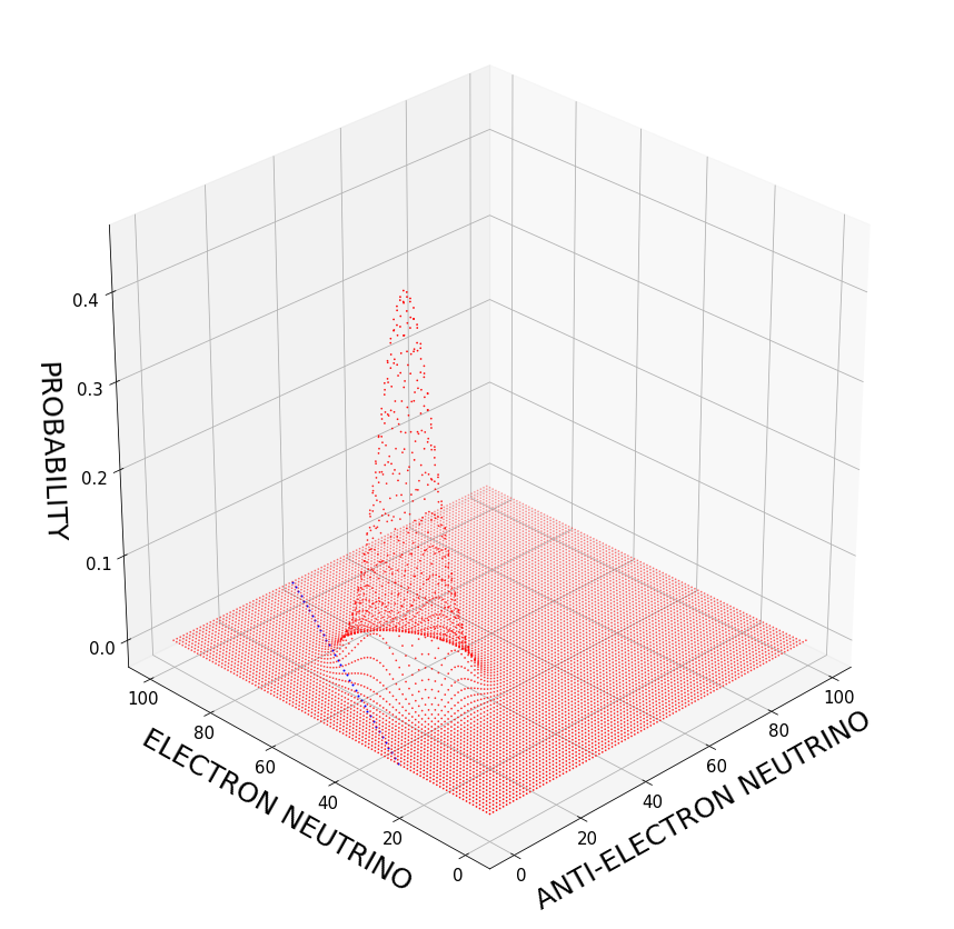
(d)

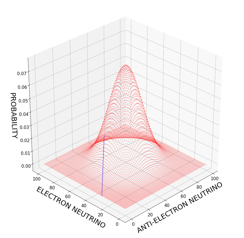
(e)

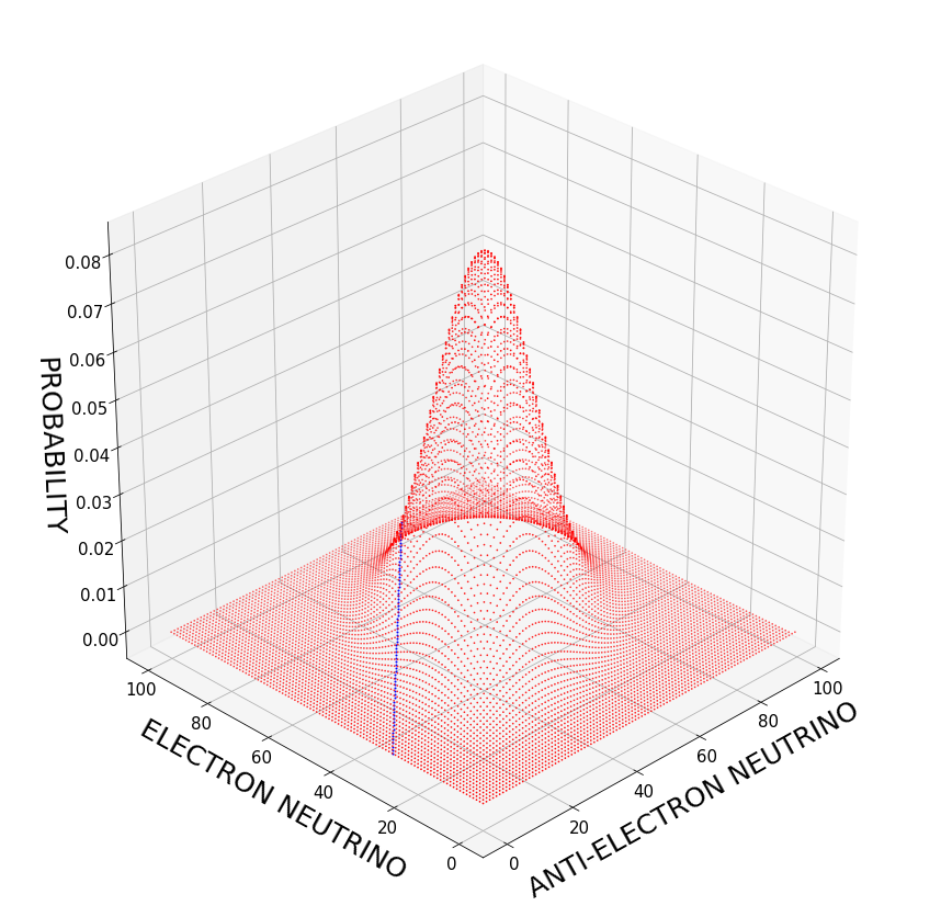
(f)

Fig. 2. In (a), the red dots are double Poisson distribution of number of $\nu_{e}$ versus the number of $\overline{\nu}_{e}$ events assuming that both distributions have an average of 51 events. The vertical probability axes are in percent. The blue dots represent the difference $n\left(\nu_{e}\right)-n\left(\overline{\nu}_{e}\right)=28$. The p-value which is the integrated probabilities of the region to the left of and including the blue dots is 0.24%. This represents statistical p-value of a test measurement of a difference of 28 events. In (b) The red dots are double Poisson distribution of number of $\nu_{e}$ (with average 51 events) versus the number of $\overline{\nu}_{e}$ events (with average of 28.5 events). The Probabilities are in percent. The blue dots represent the difference $n\left(\nu_{e}\right)-2\times n\left(\overline{\nu}_{e}\right)=28$. The p-value or integrated probabilities of the region to the left of and including the blue dots is 0.9%. This represents statistical p-value of a test measurement of a difference of n$\left(\nu_{e}\right)-2\times n\left(\overline{\nu}_{e}\right)\geq 28$ events. In (c) and (d), both Poisson distributions are smeared by 25%, however (d) has a correlation ratio of $\rho=0.5$. Note the positive correlation makes the distribution more narrow w.r.t. the blue diagonal and decreases the p-value. This is expected since this represents a cancellation of correlated neutrino and anti-neutrino errors.

The asymmetry test statistic can be calculated as,

$$A=\frac{\Delta}{N_{e}+\overline{N}_{e}}=\frac{65-37}{65+37}=\allowbreak 0.275$$ (25)

and the CPC probability of an observation is,

$$\sum_{N_{e}=0}^{\infty}\sum_{\overline{N}_{e}=0}^{\infty}\theta\left(\frac{N_{e}-\overline{N}_{e}}{N_{e}+\overline{N}_{e}}-A\right)\mathscr{P}\left(N_{e},51\right)\mathscr{P}\left(\overline{N}_{e},51\right)=0.0024$$ (26)

Note that the step functions are related,

$$\theta\left(\frac{N_{e}-\overline{N}_{e}}{N_{e}+\overline{N}_{e}}-A\right)=\theta\left(\frac{N_{e}-\overline{N}_{e}-A\left(N_{e}+\overline{N}_{e}\right)}{N_{e}+\overline{N}_{e}}\right)$$

$$=\theta\left(N_{e}-\overline{N}_{e}-A\left(N_{e}+\overline{N}_{e}\right)\right)$$ (27)

so the asymmetry statistic $A$ will have the exactly the same p-value probability results as the difference of observed events statistic $\Delta$ where $\Delta=A\left(N_{e}+\overline{N}_{e}\right)$.

Recapping the salient points, if one assumes the CPV ($\delta_{CP}=-\pi/2$) scenario is true, then there is a 59% chance of observing a measurement of at least a difference of 28 events and excluding CP conservation at the 3 standard deviation level.

5 Case II. Different Sample Sizes

In the previous sections, it was assumed the measurement efficiencies of $N_{e}$, $N_{\mu}$, $\overline{N}_{e}$ and $\overline{N}_{\mu}$ were the same. Experimentally, the muon and electron neutrino cross sections should be very similar, however the neutrino and antineutrino cross sections on the same nuclear targets will be different. Hence unless the neutrino and antineutrino integrated beam fluxes are adjusted to equalize the differences, we would expect very different sample sizes. However, this can be corrected by appropriately modifying the ratio $R$ defined in Eq. (11).

In this case, unequal neutrino and antineutrino data sizes, $N_{\mu}\neq\overline{N}_{\mu}$, are examined. Reconsider case 1 with a antineutrino sample size that is smaller and corresponds to $\overline{N}_{\mu}=500$. In this case the CPC average number of observed events is $\overline{\lambda}=\frac{51}{2}=25.5$ and a difference of neutrino and antineutrino events is considered where the antineutrino rate is scaled up by a factor 2, so the predicted difference is $65-2\times 18.5\geq 28$.

$$\sum_{N_{e}=0}^{\infty}\sum_{\overline{N}_{e}=0}^{\infty}\theta\left(N_{e}-2\times\overline{N}_{e}-28+\epsilon\right)\mathscr{P}\left(N_{e},51\right)\mathscr{P}\left(\overline{N}_{e},25.5\right)=0.0090$$ (28)

This case is displayed in Fig. 2(b). Note that step function is $N_{e}-2\times\overline{N}_{e}-28+\epsilon$ instead of $N_{e}-\overline{N}_{e}-(65-37/2+\epsilon)$. The CPC null hypothesis is along the line defined by $N_{e}=2\times\overline{N}_{e}$ and the p-value boundary is $N_{e}+28=2\times\overline{N}_{e}$ which is parallel to the CPC null hypothesis line.

A more extreme case is when $\overline{N}_{\mu}=200$, then p-value becomes,

$$\sum_{N_{e}=0}^{\infty}\sum_{\overline{N}_{e}=0}^{\infty}\theta\left(N_{e}-5\times\overline{N}_{e}-28+\epsilon\right)\mathscr{P}\left(N_{e},51\right)\mathscr{P}\left(\overline{N}_{e},10.2\right)=0.044$$ (29)

If the ratio of the neutrino to antineutrino sample sizes is $R$, then the general expression becomes,

$$\sum_{N_{e}=0}^{\infty}\sum_{\overline{N}_{e}=0}^{\infty}\theta\left(N_{e}-R\overline{N}_{e}-\Delta+\epsilon\right)\mathscr{P}\left(N_{e},\lambda\right)\mathscr{P}\left(\overline{N}_{e},\overline{\lambda}/R\right)$$ (30)

Note that the diagonal line the represents the boundary for Fig. 2(b), is has a slope of $R$ and unless $R$ is an integer, the line does not intersect all the integer points $[N_{e},\overline{N}_{e}]$ in the x-y plane in Fig. 2(b). In this case, it is not a conventional Skellam distribution that normally is an $integer$ test statistic as shown in Fig. 1(a), where the x-axis is in integer steps. If the ratio $R>1$ and not an integer ($ex.$ $R=\pi$), then it is more sensible to have a test statistic in units or steps of $R$ such that the 1-dimensional test statistic represents the summed probabilities between parallel lines with slope $R$. In this case, it is straight forward to see that these parallel lines with slope $R$ are separated by perpendicular distance, $R/\sqrt{R^{2}+1}$, which is consistent with the Skellam case when $R=1$.

6 Case III. Backgrounds

Real particle experiments typically have backgrounds or spurious events in their signal candidate event sample. This case is examined in this section. Suppose the antineutrino sample in the previous section has 10 background events. The Poisson probability will be

$$\mathscr{P}\left(N_{e},51\right)\mathscr{P}\left(\overline{N}_{e},51+10\right)$$ (31)

and the predicted difference in the number of events will be $65-\left(37+10\right)=18$.  The probability of a null hypothesis increases to

$$\sum_{N_{e}=0}^{\infty}\sum_{\overline{N}_{e}=0}^{\infty}\theta\left(N_{e}-\left(\overline{N}_{e}-10\right)-28+\epsilon\right)\mathscr{P}\left(N_{e},51\right)\mathscr{P}\left(\overline{N}_{e},51+10\right) =$$

$$\sum_{N_{e}=0}^{\infty}\sum_{\overline{N}_{e}=0}^{\infty}\theta\left(N_{e}-\overline{N}_{e}-18+\epsilon\right)\mathscr{P}\left(N_{e},51\right)\mathscr{P}\left(\overline{N}_{e},61\right)=0.0035$$ (32)

And if both neutrino and antineutrino samples had 10 background events, then the following probability for CPC is,

$$\sum_{N_{e}=0}^{\infty}\sum_{\overline{N}_{e}=0}^{\infty}\theta\left(N_{e}-\overline{N}_{e}-28+\epsilon\right)\mathscr{P}\left(N_{e},61\right)\mathscr{P}\left(\overline{N}_{e},61\right)=0.0050$$ (33)

The general form the test statistic with backgrounds will be given as before except the constants are changed by $\lambda\rightarrow\lambda+b$, $\overline{\lambda}\rightarrow\overline{\lambda}+\overline{b}$, and $\Delta\rightarrow\Delta+\left(b-\overline{b}\right)$, then,

$$\sum_{N_{e}=0}^{\infty}\sum_{\overline{N}_{e}=0}^{\infty}\theta\left(N_{e}-\overline{N}_{e}-\left(\Delta+b-\overline{b}\right)+\epsilon\right)\mathscr{P}\left(N_{e},\lambda+b\right)\mathscr{P}\left(\overline{N}_{e},\overline{\lambda}+\bar{b}\right)$$ (34)

If there is uncertainty in $\lambda$ or the background $b$, it is typically estimated as a Gaussian uncertainty $\sigma$, and the null hypothesis Poisson probability must be integrated and smeared about the $x_{0}=\lambda+b$,

$$\frac{1}{\mathscr{N}}\int_{0}^{\infty}e^{-\left(x-x_{0}\right)^{2}/2\sigma^{2}}\mathscr{P}\left(\mathrm{m,x}\right)dx=\frac{1}{N}\int_{0}^{\infty}\frac{e^{-x}x^{m}}{m!}e^{-\left(x-x_{0}\right)^{2}/2\sigma^{2}}dx$$ (35)

where, $\mathscr{N}=\int_{0}^{\infty}e^{-\left(x-x_{0}\right)^{2}/2\sigma^{2}}dx$. This integral can be solved numerically, but the definite integral[7] is related to parabolic cylindrical function $D_{n}(z)$ and has a simple closed form,

$$\begin{array}[]{c}\int_{0}^{\infty}e^{-x}x^{m}e^{-\left(x-x_{0}\right)^{2}/2\sigma^{2}}dx=\\ \\ \end{array}$$

$$\sigma^{m+1}\Gamma\left(m+1\right)exp\left(-\frac{x_{0}^{2}}{4\sigma^{2}}-\frac{x_{0}}{2}-\frac{\sigma^{2}}{4}\right)D_{-m-1}\left(-\frac{x_{0}}{\sigma}+\sigma\right)$$ (36)

Using the above, a Poisson convoluted with a Gaussian, $\widetilde{\mathscr{P}}\left(m,x_{0},\sigma\right)$ is defined as

$$\begin{array}[]{c}\widetilde{\mathscr{P}}\left(m,x_{0},\sigma\right)=\frac{1}{N}\int_{0}^{\infty}\frac{e^{-x}x^{m}}{m!}e^{-\left(x-x_{0}\right)^{2}/2\sigma^{2}}dx=\\ =\frac{\sigma^{m+1}\Gamma\left(m+1\right)}{Nm!}exp\left(-\frac{x_{0}^{2}}{4\sigma^{2}}-\frac{x_{0}}{2}-\frac{\sigma^{2}}{4}\right)D_{-m-1}\left(-\frac{x_{0}}{\sigma}+\sigma\right)\begin{array}[]{c}\\ \\ \end{array}\end{array}$$ (41)

and then the test statistic becomes,

$$\sum_{N_{e}=0}^{\infty}\sum_{\overline{N}_{e}=0}^{\infty}\theta\left(N_{e}-\overline{N}_{e}-\left(\Delta+b-\overline{b}\right)+\epsilon\right)\widetilde{\mathscr{P}}\left(N_{e},\lambda+b,\sigma\right)\mathscr{\widetilde{P}}\left(\overline{N}_{e},\overline{\lambda}+\overline{b},\overline{\sigma}\right)$$ (42)

Again, note that the double sum of the smeared Poisson is always normalized,

$$\sum_{N_{e}=0}^{\infty}\sum_{\overline{N}_{e}=0}^{\infty}\widetilde{\mathscr{P}}\left(N_{e},\lambda+b,\sigma\right)\mathscr{\widetilde{P}}\left(\overline{N}_{e},\lambda+\overline{b},\overline{\sigma}\right)$$

$$=\sum_{N_{e}=0}^{\infty}\widetilde{\mathscr{P}}\left(N_{e},\lambda+b,\sigma\right)\sum_{\overline{N}_{e}=0}^{\infty}\mathscr{\widetilde{P}}\left(\overline{N}_{e},\lambda+\overline{b},\overline{\sigma}\right)$$

$$=\frac{1}{\mathscr{N}}\int_{0}^{\infty}\left(\sum_{n=0}^{\infty}\frac{e^{-\lambda}\lambda^{n}}{n!}\right)e^{-\left(\lambda-\lambda_{0}\right)^{2}/2\sigma^{2}}d\lambda$$

$$\times\frac{1}{\overline{\mathscr{N}}}\int_{0}^{\infty}\left(\sum_{m=0}^{\infty}\frac{e^{-\overline{\lambda}}\overline{\lambda}^{m}}{m!}\right)e^{-\left(\overline{\lambda}-\overline{\lambda}_{0}\right)^{2}/2\overline{\sigma}^{2}}d\overline{\lambda}=1$$ (43)

If the errors in the neutrino and antineutrino Poisson’s are correlated, $\rho=\frac{\left\langle\sigma\overline{\sigma}\right\rangle}{\sigma\overline{\sigma}}\neq 0$, then a 2 dimensional integral with correlations is formed. The correlated errors can include the flux errors on the neutrino and antineutrino beams, the cross section uncertainties and the detector efficiency uncertainties. The separate integrals becomes a Gaussian bivariate distribution,

$$\frac{1}{\overline{\mathscr{N}}}\int_{0}^{\infty}\int_{0}^{\infty}\frac{e^{-x}x^{m}}{m!}\frac{e^{-y}y^{n}}{n!}$$

$$\times e^{\left(-\frac{1}{1-\rho^{2}}\left[-\frac{1}{2}\left(x-\lambda\right)^{2}/\sigma^{2}-\frac{1}{2}\left(y-\overline{\lambda}\right)^{2}/\overline{\sigma}^{2}+\rho\left(x-\lambda\right)\left(y-\overline{\lambda}\right)/\sigma\overline{\sigma}\right]\right)}dxdy$$ (44)

If the covariance is positive, $\rho>0$, then the p-value will be reduced since the principle axis of the error elipse that is parallel to the boundary of the p-value region will be narrower. In Figs. 2(c)-(d), are the results for 25% and 25% with correlation errors of $\rho=0.5,$ respectively.

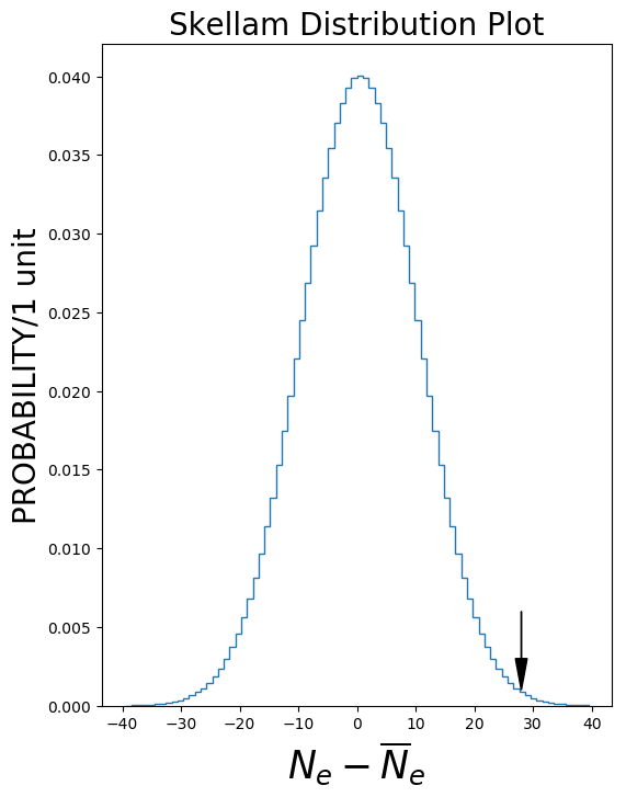
(g)

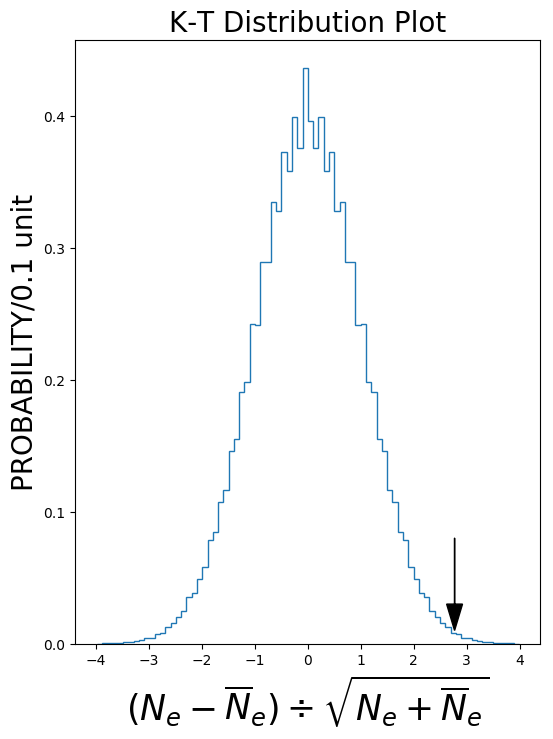
(h)

Fig. 3. In (a) is the Skellam distribution of the double Poisson distributions created from Fig. 2(a). The arrow at $N_{e}-\overline{N}_{e}=28$ corresponds to a p-value of 0.0024. The K-T test statistic of the difference in standard deviations is plotted in (b). The arrow at $\left(N_{e}-\overline{N}_{e}\right)/\sqrt{N_{e}+\overline{N}_{e}}=2.77$ corresponds to a p-value of 0.0027.

7 Case IV Different Sample Sizes with backgrounds.

Next, cases that include backgrounds and allows for difference sample sizes are presented. Starting again with case 1, it is assumed that the antineutrino events reduced by a factor $R=2$ and the antineutrino background is 10 events.  In this case there are $N_{\mu}=1000$, $\overline{N}_{\mu}=\frac{N_{\mu}}{2}=500$ and antineutrino background, $\overline{b}=10$. The CPC averages are $\lambda=51$ and $\overline{\lambda}=\lambda/R+\overline{b}=35.5$.  The expected difference (if $\delta_{CP}=-\pi/2$) is $65-R\times\left(37/R+\overline{b}\right)=65-2\times\left(37/2+10\right)=8$. The expression for this example becomes

$$\sum_{N_{e}=0}^{\infty}\sum_{\overline{N}_{e}=0}^{\infty}\theta\left(N_{e}-2\times\overline{N}_{e}-8+\epsilon\right)\mathscr{P}\left(N_{e},35.5\right)\mathscr{P}\left(\overline{N}_{e},35.5\right)$$ (45)

and a general expression of the p-value for a null hypothesis test is,

$$\sum_{N_{e}=0}^{\infty}\sum_{\overline{N}_{e}=0}^{\infty}\theta\left(N_{e}-R\times\overline{N}_{e}-\Delta+\epsilon\right)\mathscr{P}\left(N_{e},\lambda+b\right)\mathscr{P}\left(\overline{N}_{e},\overline{\lambda}/R+\overline{b}\right)$$ (46)

where $\Delta=N_{e}-R\times\overline{N}_{e}$ is the observed difference, $R$ is the ratio of $N_{\mu}/\overline{N}_{\mu}$ sample sizes, $\lambda+b$ is the predicted $N_{e}$ null hypothesis events, and $\overline{\lambda}/R+\overline{b}$ is the predicted $\overline{N}_{e}$ null hypothesis events. The relations between the CP conserving combination of $N_{e}$ and $\overline{N}_{e}$ events, the observed difference $\Delta$, and the p-value region is presented schematically in Fig. 4. The p-value will be the sum of the double Poisson terms $\mathscr{P}\left(N_{e},\lambda+b\right)\mathscr{P}\left(\overline{N}_{e},\overline{\lambda}/R+\overline{b}\right)$ in the light red region.

Fig 4. The CPC events satisfy $N_{e}-R\cdot\overline{N}_{e}=b-\overline{b}$ and will lie on the blue line. The events that have an observed difference of $N_{e}-R\cdot\overline{N}_{e}=\Delta^{meas}$ will lie on the dashed red line. The light red solid colored region above the dash red line is p-value region. The red dashed line p-value boundary has a slope R and is parallel to the blue line.

If the ratio $R$ has Gaussian uncertainty, then it can also be varied to get an averaged p-value. If the predicted number of events have Gaussian uncertainties, then the Poisson terms are replaced with the Gaussian smeared Poisson terms. A similar expression for A is,

$$\sum_{N_{e}=0}^{\infty}\sum_{\overline{N}_{e}=0}^{\infty}\theta\left(\frac{\left(N_{e}-b\right)-R\times\left(\overline{N}_{e}-\overline{b}\right)}{\left(N_{e}-b\right)+R\times\left(\overline{N}_{e}-\overline{b}\right)}-A\right)$$

$$\times\mathscr{P}\left(N_{e},\lambda/R+b\right)\mathscr{P}\left(\overline{N}_{e},\lambda/R+\overline{b}\right)$$ (47)

where $A$ is the measured asymmetry.

Fig. 5. The standard deviation distributions of the double Poisson distributions using the K-T test statistic. The x and y axes are in standard deviation units of $N_{e}/\sqrt{N_{e}+\overline{N}_{e}}$ and $\overline{N}_{e}/\sqrt{N_{e}+\overline{N}_{e}}$ , respectively. The Poisson distribution (red dots) has $\lambda=51$ and the blue boundary corresponds to observed $\Delta=N_{e}-\overline{N}_{e}=65-37=28$ with a p-value of $0.27\%$.

8 Case V Unknown Oscillation Probabilities

In the previous sections, a value of the CPC probability $\lambda$ was assumed to be known and was used in the null hypothesis calculations. In principle, the average of observed measurements of $N_{e}$ and $\overline{N}_{e}$ can be used as a statistical estimate for $\lambda$ and instead of using the difference test statistic, $N_{e}-\overline{N}_{e}$, a better test statistic is, $\frac{N_{e}-\overline{N}_{e}}{\sqrt{N_{e}+\overline{N}_{e}}}$, where the initial muon neutrino samples are assumed to be equal, $N_{\mu}=\overline{N}_{\mu}$. This statistic by Krishnamoorthy and Thomson (K-T)[8] represents the difference in units of standard deviations. If the best estimate of the CPC null hypothesis $\lambda$ is the average of the observed events, $\left(N_{e}+\overline{N}_{e}\right)/2$, then $\frac{N_{e}-\overline{N}_{e}}{\sqrt{N_{e}+\overline{N}_{e}}}$ is proportional to the difference in units of standard deviations. In the limit that the Poisson distribution becomes a Normal distribution it is noted that the p-value boundaries are in units of standard deviations and the p-value will not depend on a particular value of $\lambda$.

Reconsider Case I, by assuming the observed events are $N_{e}=65$ and $\overline{N}_{e}=37$ and using the test statistic $\frac{N_{e}-\overline{N}_{e}}{\sqrt{N_{e}+\overline{N}_{e}}}$. The p-value boundary point is at $N_{e}/\sqrt{N_{e}+\overline{N}_{e}}=6.44$ and $\overline{N}_{e}/\sqrt{N_{e}+\overline{N}_{e}}=3.66$ which has a difference of 2.772. The p-value is now estimated by assuming the unknown CP conserving probability is given by the estimate $\lambda=\left(N_{e}+\overline{N}_{e}\right)/2$ or 51.

$$\sum_{N_{e}=0}^{\infty}\sum_{\overline{N}_{e}=0}^{\infty}\theta\left((N_{e}-\overline{N}_{e})/\sqrt{(N_{e}+\overline{N}_{e}}-2.772+\epsilon\right)\mathscr{P}\left(N_{e},51\right)\mathscr{P}\left(\overline{N}_{e},51\right)=0.00271$$ (48)

The double Poisson is plotted as a function of $N_{e}/\sqrt{N_{e}+\overline{N}_{e}}$ and $\overline{N}_{e}/\sqrt{N_{e}+\overline{N}_{e}}$ with red dots and the p-value boundary in blue dots that is a 45 degree line that lies on the boundary point at $N_{e}/\sqrt{N_{e}+\overline{N}_{e}}=6.44$ and $\overline{N}_{e}/\sqrt{N_{e}+\overline{N}_{e}}=3.66$ in Fig. 5. The resulting p-value is $0.271\%$, which is very close to the results of Case 1 which obtained 0.242%. This test statistic is largely insensitive to the true value of $\lambda$. This is readily verified in our example by recalculating the p-values for different assumed values of $\lambda$ of 41 or 61 and obtaining the corresponding p-values of 0.265% or 0.274%, respectively.

This test statistic can be applied to Case II of different sample sizes. In this case $N_{e}=65$ and $\overline{N}_{e}=37$/2 events are observed and the p-value boundary point is $N_{e}/\sqrt{N_{e}+4\times\overline{N}_{e}}=5.51$ and $2\times\overline{N}_{e}/\sqrt{N_{e}+4\times\overline{N}_{e}}=3.14$ and the difference is 2.375. The p-value becomes,

$$\sum_{N_{e}=0}^{\infty}\sum_{\overline{N}_{e}=0}^{\infty}\theta\left((N_{e}-2\times\overline{N}_{e})/\sqrt{N_{e}+4\times\overline{N}_{e}}-2.375+\epsilon\right)\mathscr{P}\left(N_{e},51\right)\mathscr{P}\left(\overline{N}_{e},25.5\right)=1.36\%$$ (49)

The p-value increases to $1.36\%$ compared to the value of $0.9\%$ in Case II. If one assumes values of $\lambda$ of 41 or 61, the resulting p-values are 1.31% or 1.41%, respectively.

Next we apply the statistic to Case III with backgrounds. In this case, $N_{e}=65$ and $\overline{N}_{e}=37$+10 are observed events and the p-value boundary is $N_{e}/\sqrt{N_{e}+\overline{N}_{e}}=6.14$ and $\overline{N}_{e}/\sqrt{N_{e}+\overline{N}_{e}}=4.44$. The difference is 1.70. The p-value becomes,

$$\sum_{N_{e}=0}^{\infty}\sum_{\overline{N}_{e}=0}^{\infty}\theta\left((N_{e}-\overline{N}_{e})/\sqrt{N_{e}+\overline{N}_{e}}-1.70+\epsilon\right)\mathscr{P}\left(N_{e},51\right)\mathscr{P}\left(\overline{N}_{e},51+10\right)=0.41\%$$ (50)

The p-value slightly increases to $0.41\%$ compared to the value $0.35\%$ in Case III. If different assumed values of $\lambda$ of 41 or 61 are used, the resulting p-values are slightly changed to 0.31% or 0.51%, respectively.

9 Combining Different Experiments

As different long baseline neutrino experiments add more data and perform neutrino and antineutrino oscillation measurements, the results ($ex.$ from experiments A and B) could be combined to obtain a joint p-value test of the null hypothesis. Assuming both experiments have a CPC null hypothesis with a common value of $\lambda$ and one-sided distributions on the same side, then p-values could be extracted from two 1-dimensional Skellam distributions, $P_{a}^{SK}\left(\Delta_{a}\right)$ and $P_{b}^{SK}\left(\Delta_{b}\right)$. The problem of combining p-values from two independent measurements has been solved by R. A. Fisher[9] and a simple derivation[10] is given here. Since the p-value of the null hypotheses represents flat distributions of p-value_a and p-value_b, where each can vary from 0 to 1, a unit square can be formed with axes of these two probabilities. So unlike the probabilities in Fig. 1(b) and Figs. 2 (a)-(d), the joint p-value probabilities are flat or constant areas on the p-value_a vs p-value_b plane as shown in Fig. 6 (a). Suppose experiment A measures a p-value $p^{\prime}_{a}$ and experiment B measures a p-value $p^{\prime}_{b}$. These two values form a p-value boundary point. Their product is $c=p^{\prime}_{a}p^{\prime}_{b}$ and this forms inside the unit square a boundary defined by the curve, $p_{b}=c/p_{a}$ as shown in Fig. 6 (a) where the boundary point lies on the curve defined by $c=p^{\prime}_{a}p^{\prime}_{b}$. The p-value formed by combining these 2 experiments is given by the region or area inside the unit square corresponding to $p_{a}p_{b}\leq c$ which is below and to the left of this boundary line. This area equals $-c\ \ln c+c$ and represents the extreme p-value. The area above and to the right of the boundary curve is 1$-$(p-value). The p-values whose probabilities correspond to one sided 1, 2 and 3 standard deviations of normal probabilities are presented in Fig. 6 (a). Suppose there are two imaginary p-value measurements of 0.4 and 0.0925 from different experiments. This result appears as a green square in Fig. 6 (a). These measurements produce the green boundary line whose lower left area corresponds to 0.159 which is the joint p-value. Since $c=0.4\times 0.0925=0.037$, it is noted that the same combined p-value would be achieved with two imaginery p-values measurements of $0.37$ and $0.1$. The natural log of each p-value can be also be plotted as shown in Fig. 6 (b). The curves become simple diagonal lines and the region above and to the right of the diagonal lines represents 1$-$(p-value) region. This can be generalized to n experiments where the probability is an n dimensional volume and the n-1 dimensional hyper-surface defined by $c=p_{1}...p_{n}$ which forms the boundary separating the p-value region and the 1$-$(p-value) region.

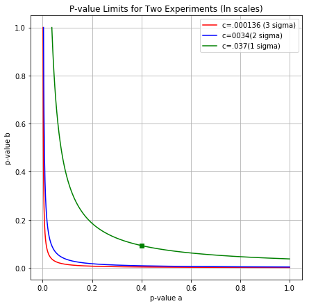
(i)

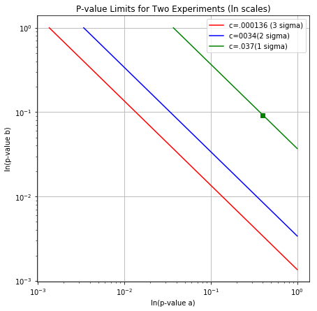
(j)

Fig. 6. In (a) is the unit square of p-value₁ versus p-value₂ with green, blue and red curves representing different probability boundaries for c = 0.037, 0.0034 and 0.000136, respectively. The areas below and to the left of each curve is 0.159, 0.0227 and 0.00135, respectively. If experiment 1 and 2 obtained p-values of .4 and .0925, respectively, then $c=0.4\times 0.0925=0.037$ which corresponds to the green dot, that lies on the green curve that represents the equation $p-value_{2}=0.037/p-value_{1}$. The p-value that combines the two experiments is represented by the area to the left and below the green curve that equals $-c\ \ln c+c=0.159$ and which is the one sided probability for 1 sigma normal distribution. The other blue and red boundaries correspond to the one sided 2 and 3 sigma normal probabilities, respectively. For small p-values, a more useful graphic is the plot of ln($p-value_{1}$) vs ln($p-value_{2}$) which forms straight line diagonal boundaries at 45^∘. This is shown in (b), where the upper left area with respect to these boundaries represents the 1$-$(p-value) for the two experiments.

10 Discussion and Summary

In this paper, the hypothesis of CP conservation that the neutrino and antineutrino electron appearance oscillation probabilities are equal, is tested by counting the number of neutrino and antineutrino events. The inputs to this test static include the observed $N_{e}$ and $\overline{N}_{e}$ and the unoscillated $N_{\mu}$ and $\overline{N}_{\mu}$ , the predicted null hypothesis rates $\lambda+b$ and $\overline{\lambda}+\overline{b}$ , and the ratio R that depends on the neutrino and antineutrino cross sections, the estimated backgrounds, the reconstruction efficiencies and relative integrated $\nu$ and $\overline{\nu}$ fluxes. The cases with equal data samples, with/without backgrounds, unequal data samples, smeared background rates and CP conserved oscillation probability rates and unknown CP conserved oscillation rates were discussed. The p-values can be recalculated as more data is accumulated in experiments and displayed in modified Skellam distributions or as 3-d plots of probabilities with p-value boundaries. In addition the p-values from 2 different experiments can be readily combined to produce a joint p-value to test the null CP conserving hypothesis in neutrino oscillations. The predictions in this note will be useful to check more sophisticated and complex statistical tests of CP violation that fit neutrino parameters.

Finally, methods in this paper can be used to predict the CP conserving p-value tests assuming a specific set of neutrino mixing parameters with future scenarios of different amounts of neutrino and antineutrino beam data. This could be advantageous to optimize the experimental test for CP violation by varying the amount or mix of neutrino and antineutrino beam running.

11 Acknowledgements

This work was supported by the U.S. Department of Energy, Office of Science, under Award Number DE-FOA-0001604. We acknowledge support from the Program of Research and Scholarly Excellence in High Energy Physics and Particle Astrophysics at Colorado State University and we thank Prof. Donald Estep for reading an early draft.

12 Appendix

The appendix describes the dependence between the reconstructed number of events, backgrounds, oscillation probabilities, cross sections, neutrino flux and reconstruction efficiencies. This section considers the case (1) where the neutrino and antineutrino fluxes peak at the same one energy and the case (2) where the neutrino and the antineutrino fluxes are spread over a range of energies. These relations will require careful Monte Carlo simulations of the CPC modeling, backgrounds, detector resolutions and efficiencies and neutrino beam fluxes.

Let’s first define the relation of the fluxes and observables. The number of unoscillated muon neutrinos and antineutrinos in our detectors are;

$$\begin{array}[]{c}\int\Phi^{\prime}\left(E_{\nu_{\mu}}\right)dE_{\nu_{\mu}}=n\left(\nu_{\mu}\right)\\ \int\overline{\Phi}^{\prime}\left(E_{\overline{\nu}_{\mu}}\right)dE_{\overline{\nu}_{\mu}}=n\left(\overline{\nu}_{\mu}\right)\end{array}$$ (51)

where the neutrino differential integrated flux is $\Phi^{\prime}\left(E_{\nu}\right)\equiv\partial\Phi\left(E_{\nu}\right)/\partial E_{\nu}$ and the analogous antineutrino barred quantities. The produced number of oscillated electron appearance neutrinos are;

$$\begin{array}[]{c}\int P\left(E_{\nu_{\mu}}\right)\times\Phi^{\prime}\left(E_{\nu_{\mu}}\right)dE_{\nu_{\mu}}=n\left(\nu_{e}\right)\\ \int\overline{P}\left(E_{\overline{\nu}_{\mu}}\right)\times\overline{\Phi}^{\prime}\left(E_{\overline{\nu}_{\mu}}\right)dE_{\overline{\nu}_{\mu}}=n\left(\overline{\nu}_{e}\right)\end{array}$$ (52)

where the PMNS probabilities for $P\left(\nu_{\mu}\rightarrow\nu_{e}\right)$ and $\overline{P}\left(\overline{\nu}_{\mu}\rightarrow\overline{\nu}_{e}\right)$ depend on all parameters,

$$\begin{array}[]{c}P\left(L/E,\theta_{ij},\Delta m_{ij}^{2},\delta_{CP},MH\right)\\ \overline{P}\left(L/E,\theta_{ij},\Delta m_{ij}^{2},\delta_{CP},MH\right)\end{array}$$ (53)

and where MH denotes the mass hierarchy. The true (or produced) and observed number of appearance $e^{+}/e^{-}$ events at the far detector are,

$$\begin{array}[]{c}\int\sigma\left(E_{\nu}\right)\times P\left(E_{\nu_{\mu}}\right)\times\Phi^{\prime}\left(E_{\nu}\right)dE_{\nu}=n^{true}\left(e^{-}\right)=\frac{n^{obs}\left(e^{-}\right)}{\epsilon_{e}}\\ \int\overline{\sigma}\left(E_{\overline{\nu}}\right)\times\overline{P}\left(E_{\overline{\nu}_{\mu}}\right)\times\overline{\Phi}^{\prime}\left(E_{\overline{\nu}}\right)dE_{\overline{\nu}}=n^{true}\left(e^{+}\right)=\frac{n^{obs}\left(e^{+}\right)}{\epsilon_{\overline{e}}}\end{array}$$ (54)

where $\epsilon_{e}$ and $\epsilon_{\overline{e}}$ are the detection and reconstruction efficiencies and where we use notation $n^{obs}\equiv N^{data}-B^{MC}$. The number of predicted data events are then,

$$\begin{array}[]{c}\lambda+b=\epsilon_{e}\int\sigma\left(E_{\nu}\right)\times P\left(E_{\nu_{\mu}}\right)\times\Phi^{\prime}\left(E_{\nu}\right)dE_{\nu}+B^{MC}\\ \overline{\lambda}+\overline{b}=\epsilon_{\overline{e}}\int\overline{\sigma}\left(E_{\overline{\nu}}\right)\times\overline{P}\left(E_{\overline{\nu}_{\mu}}\right)\times\overline{\Phi}^{\prime}\left(E_{\overline{\nu}}\right)dE_{\overline{\nu}}+\overline{B}^{MC}\end{array}$$ (55)

The number of unoscillated muon $\mu^{+}/\mu^{-}$ true (or produced) events at the near detector extrapolated to the far detector are

$$\begin{array}[]{c}\int\sigma\left(E_{\nu}\right)\times\Phi^{\prime}\left(E_{\nu}\right)dE_{\nu}=n^{true}\left(\mu^{-}\right)=\frac{n^{obs}\left(\mu^{-}\right)}{\epsilon_{\mu}}\\ \int\overline{\sigma}\left(E_{\overline{\nu}}\right)\times\overline{\Phi}^{\prime}\left(E_{\overline{\nu}}\right)dE_{\overline{\nu}}=n^{true}\left(\mu^{+}\right)=\frac{n^{obs}\left(\mu^{+}\right)}{\epsilon_{\overline{\mu}}}\end{array}$$ (56)

where we assume electron-muon universality, $\sigma_{e}\left(E_{\nu}\right)=\sigma_{\mu}\left(E_{\nu}\right)=\sigma\left(E_{\nu}\right)$ and $\overline{\sigma}_{e}\left(E_{\overline{\nu}}\right)=\overline{\sigma}_{\mu}\left(E_{\overline{\nu}}\right)=\overline{\sigma}\left(E_{\overline{\nu}}\right)$ and the efficiencies are $\epsilon_{\mu}$ and $\epsilon_{\overline{\mu}}$ . The ratio of muon neutrino/antineutrino corrected event rates measured at the near detector is,

$$r=\frac{\int\overline{\sigma}\left(E_{\overline{\nu}}\right)\overline{\Phi}^{\prime}\left(E_{\overline{\nu}}\right)dE_{\overline{\nu}}}{\int\sigma\left(E_{\nu}\right)\Phi^{\prime}\left(E_{\nu}\right)dE_{\nu}}$$ (57)

In order to test CP violation, we require $P\left(E\right)=\overline{P}\left(E\right)$ for all values of energy $E$.

Case (1) Suppose we have a neutrino and antineutrino beam at the same one energy given by a Dirac delta function, $\Phi^{\prime}\left(E_{\nu}\right)=\delta\left(E_{\nu}-E_{0}\right)$, we can readily see

$$\begin{array}[]{c}P\left(E_{0}\right)=\frac{\Phi_{e}\left(E_{0}\right)}{\Phi_{\mu}\left(E_{0}\right)}=\frac{\sigma_{e}\left(E_{0}\right)\times P\left(E_{0}\right)\times\Phi_{\mu}\left(E_{0}\right)}{\sigma_{\mu}\left(E_{0}\right)\times\Phi_{\mu}\left(E_{0}\right)}=\frac{n^{true}\left(e^{-}\right)}{n^{true}\left(\mu^{-}\right)}\\ \overline{P}\left(E_{0}\right)=\frac{\overline{\Phi}_{e}\left(E_{0}\right)}{\overline{\Phi}_{\mu}\left(E_{0}\right)}=\frac{\overline{\sigma}_{e}\left(E_{0}\right)\times\overline{P}\left(E_{0}\right)\times\overline{\Phi}_{\mu}\left(E_{0}\right)}{\overline{\sigma}_{\mu}\left(E_{0}\right)\times\overline{\Phi}_{\mu}\left(E_{0}\right)}=\frac{n^{true}\left(e^{+}\right)}{n^{true}\left(\mu^{+}\right)}\end{array}$$ (58)

Then $P\left(E_{0}\right)=\overline{P}\left(E_{0}\right)$ can be tested by using our observed results and checking for inequality of,

$$\frac{n^{obs}\left(e^{-}\right)/\epsilon_{e}}{n^{obs}\left(\mu^{-}\right)/\epsilon_{\mu}}\neq\frac{n^{obs}\left(e^{+}\right)/\epsilon_{\overline{e}}}{n^{obs}\left(\mu^{+}\right)/\epsilon_{\overline{\mu}}}$$

$$\frac{n^{obs}\left(e^{+}\right)/\epsilon_{\overline{e}}}{n^{obs}\left(e^{-}\right)/\epsilon_{e}}\neq\frac{n^{obs}\left(\mu^{+}\right)/\epsilon_{\overline{\mu}}}{n^{obs}\left(\mu^{-}\right)/\epsilon_{\mu}}=r$$

$$n^{obs}\left(e^{+}\right)-R\times n^{obs}\left(e^{-}\right)\neq 0$$ (59)

where $R=r\times\frac{\epsilon_{\overline{e}}}{\epsilon_{e}}$.

Case (2), Suppose we consider that the flux energy is not a Delta function and has a flux that is spreadout and smeared as a function of neutrino/antineutrino energy and they do not have the same shape. Then we need to be more careful since even if $P=\overline{P}$, is true at all energies, then it is NOT necessarily true that,

$$\frac{\int\overline{\sigma}\left(E_{\overline{\nu}}\right)\times\overline{P}\left(E_{\overline{\nu}_{\mu}}\right)\times\overline{\Phi}^{\prime}\left(E_{\overline{\nu}}\right)dE_{\overline{\nu}}}{\int\overline{\sigma}\left(E_{\overline{\nu}}\right)\times\overline{\Phi}^{\prime}\left(E_{\overline{\nu}}\right)dE_{\overline{\nu}}}=\frac{\int\sigma\left(E_{\nu}\right)\times P\left(E_{\nu_{\mu}}\right)\times\Phi^{\prime}\left(E_{\nu}\right)dE_{\nu}}{\int\sigma\left(E_{\nu}\right)\times\Phi^{\prime}\left(E_{\nu}\right)dE_{\nu}}$$ (60)

since the shape of the neutrino and antineutrino flux distribution as a function of energies are not exactly the same and the cross sections are not the same.

To allow for this case (2), we calculate the MC probability (assuming the CP conserving case of $P_{CPC}\left(E\right)=\overline{P}_{CPC}\left(E\right)$ and including MSW effects if necessary) averaged over neutrino and antineutrino flux energies, so we can add a correction or fudge factor $\gamma$ which we hope should be very close to unity. Suppose the MC determines the averaged CPC probabilities,

$$\begin{array}[]{c}\left\langle P_{CPC}\left(E_{\nu_{\mu}}\right)\right\rangle=\frac{\int\sigma_{e}\left(E_{\nu}\right)\times P_{CPC}\left(E_{\nu_{\mu}}\right)\times\Phi^{\prime}\left(E_{\nu}\right)dE_{\nu}}{\int\sigma_{\mu}\left(E_{\nu}\right)\times\Phi^{\prime}\left(E_{\nu}\right)dE_{\nu}}\\ \left\langle\overline{P}_{CPC}\left(E_{\overline{\nu}_{\mu}}\right)\right\rangle=\frac{\int\overline{\sigma}_{e}\left(E_{\overline{\nu}}\right)\times P_{CPC}\left(E_{\overline{\nu}_{\mu}}\right)\times\overline{\Phi}^{\prime}\left(E_{\overline{\nu}}\right)dE_{\overline{\nu}}}{\int\overline{\sigma}_{\mu}\left(E_{\overline{\nu}}\right)\times\overline{\Phi}^{\prime}\left(E_{\overline{\nu}}\right)dE_{\overline{\nu}}}\end{array}$$ (61)

$$\gamma\equiv\left\langle\overline{P}_{CPC}\left(E_{\overline{\nu}_{\mu}}\right)\right\rangle/\left\langle P_{CPC}\left(E_{\nu_{\mu}}\right)\right\rangle$$ (62)

If we now measure or count the four observeables $n^{obs}\left(e^{+}\right)$ and $n^{obs}\left(e^{-}\right)$ at the far detector and $n^{obs}\left(\mu^{+}\right)$ and $n^{obs}\left(\mu^{-}\right)$ at the near detector, the test of CPV test becomes checking if the following relations are unequal,

$$\gamma\neq\frac{\left(\frac{n^{obs}\left(e^{+}\right)/\epsilon_{\overline{e}}}{n^{obs}\left(\mu^{+}\right)/\epsilon_{\overline{\mu}}}\right)}{\left(\frac{n^{obs}\left(e^{-}\right)/\epsilon_{e}}{n^{obs}\left(\mu^{-}\right)/\epsilon_{\mu}}\right)}$$ (63)

or

$$\frac{1}{\gamma}\frac{n^{obs}\left(e^{+}\right)/\epsilon_{\overline{e}}}{n^{obs}\left(e^{-}\right)/\epsilon_{e}}\neq\frac{n^{obs}\left(\mu^{+}\right)/\epsilon_{\overline{\mu}}}{n^{obs}\left(\mu^{-}\right)/\epsilon_{\mu}}=r$$ (64)

or

$$n^{obs}\left(e^{+}\right)-R\times n^{obs}\left(e^{-}\right)\neq 0$$ (65)

where the $R$ from Eq. (10), becomes $R=\gamma\times r\times\frac{\epsilon_{\overline{e}}}{\epsilon_{e}}$. Note in the final p-value calculations, the R uncertainties should be included through the gaussian smearing of the Poisson distribution with the $\sigma\left(\lambda+b\right)$ and $\bar{\sigma}\left(\overline{\lambda}+\overline{b}\right)$ standard deviations and the correlation parameter $\rho$ in Eqn. 44.

13 References

References

• [1] Section 14. Neutrino Mass, Mixing and Oscillations, in C. Patrignani et. al. (Particle Data Group Collaboration), Chin. Phys. ${\bf C38}$, 100001(2016) and 2017 update. A recent review is given in C. Giganti, S. Lavignac and M. Zito, Nucl. Instr. and Meth. in Phys. Res. ${\bf A98}$ (2018) 1.
• [2] K. Abe et al. (T2K Collaboration) Nucl. Instrum. Meth. ${\bf A659}$, 106 (2011) and P. Adamson et al. (NOvA Collaboration), Nucl. Instrum. Meth. ${\bf A806}$, 279 (2016); NuMI Technical Design Handbook, FERMILABDESIGN-1998-01.
• [3] R. Acciarri et al. (DUNE Collaboration), arXiv:1601.02984 [physics.ins-det] and K. Abe et al. (HyperK Collaboration), KEK preprint 2016-21.
• [4] The MSW effect for neutrinos/antineutrinos travelling in dense matter can cause a difference in the electron neutrino appearance probabilities, see S. P. Mikheyev and A. Yu. Smirnov, Soviet Journal of Nuclear Physics. ${\bf 42}$ (6):913-91 (1985) and L. Wolfenstein, Phys. Rev. ${\bf D17}$ (1978) 2369.
• [5] J. G. Skellam, Journal of the Royal Statistical Society Series A Statistics in Society,${\bf 109}$ (1946) 3, 296.
• [6] For testing dodder seeds in a bag of clover seeds, see J. Przyborowski and H. Wilenski, Biometrika 31 (1940) 313; For the ratio of Poisson means, see D. G. Chapman, Ann. Inst. Stat. Math (Tokyo) 4 (1952) 45-49 and R. D. Cousins, Nucl. Instr. and Meth. in Phys. Res. ${\bf A417}$ (1998) 391; Modeling of sports data is given in D. Karlis and I. Ntzoufras, The Statistician, ${\bf 52}$ (2003) 381.
• [7] see section 3.462 in I . Gradshyteyn, I. Ryzhik, and A. Jeffrey, Table of Integrals, Series, and Products, 5th ed., 1994, Academic Press.
• [8] K. Krishnamoorthy and J. Thomson, Journal of Statistical Planning and Inference 119 (2004) 23 – 35. This paper describes the test based on estimated p-values of a standardized difference. Also see an earlier form of this statistical test for Binomial distributions in B. E. Storer and C. Kim, Jour. Amer. Stat. Association, 85 (1990) 146–155.
• [9] R. A. Fisher, Statistical Methods for Research Workers, 11th ed. (1950), p. 99 ; also see M. B. Brown, Biometrics Journal, 31 (1975) 4, 982 for combining non-independent p-value tests.
• [10] R. C. Elston, Biometrics Journal, 33 (1991) 3, 339.