A Hybrid RF-VLC System for Energy Efficient Wireless Access

Abstract

In this paper, we propose a new paradigm in designing and realizing energy efficient wireless indoor access networks, namely, a hybrid system enabled by traditional RF access, such as WiFi, as well as the emerging visible light communication (VLC). VLC facilitates the great advantage of being able to jointly perform illumination and communications, and little extra power beyond illumination is required to empower communications, thus rendering wireless access with almost zero power consumption. On the other hand, when illumination is not required from the light source, the energy consumed by VLC could be more than that consumed by the RF. By capitalizing on the above properties, the proposed hybrid RF-VLC system is more energy efficient and more adaptive to the illumination conditions than the individual VLC or RF systems. To demonstrate the viability of the proposed system, we first formulate the problem of minimizing the power consumption of the hybrid RF-VLC system while satisfying the users requests and maintaining acceptable level of illumination, which is NP-complete. Therefore, we divide the problem into two subproblems. In the first subproblems, we determine the set of VLC access points (AP) that needs to be turned on to satisfy the illumination requirements. Given this set, we turn our attention to satisfying the users’ requests for real-time communications, and we propose a randomized online algorithm that, against an oblivious adversary, achieves a competitive ratio of $\log(N)\log(M)$ with probability of success $(1-\frac{1}{N})$, where $N$ is the number of users and $M$ is the number of VLC and RF APs. We also show that the best online algorithm to solve this problem can achieve a competitive ratio of $\log(M)$. Simulation results further demonstrate the advantages of the hybrid system.

I Introduction

The access portion of the Internet is becoming predominantly wireless. Cellular networks and wireless indoor networks, such as WiFi, are becoming the predominant choice of wireless access. Watching HD streaming videos and accessing cloud-based services are the main user activities that rapidly consume the data capacity. They will continue to be the major capacity consuming activities in the future. Moreover, activities linked with high data rate wireless traffic are stationary and typically occur in fixed wireless access scenarios [1]. Reported data indicate that a majority of IP-traffic usage occurs indoors (70% indoors and only 30% of the traffic is served outdoors [2]). According to Ericsson report [3], we spend 90% of our time indoors, and 80% of the mobile Internet access traffic happens indoors [4, 5]. This percentage will only increase as 54% of the cellular traffic is expected to be offloaded to WiFi by 2019 [6]. It is expected that 87% of the companies would switch cellular providers by 2019 for better indoor coverage [4].

The rapid increase in wireless traffic is highly coupled with an increase in energy consumption. In 2011, energy consumption of Internet in the US was larger than that of the whole automotive industry and about half that of the chemical industry, as mentioned in a CNN report [7]. Furthermore, Internet traffic is estimated to grow by a factor of 10 during 2013-2018 [8], and thus incurs more energy consumption. According to [9], the number of only public WiFi routers in the world, such as routers in shopping malls and coffee shops, will be 340 million in 2018. While being idle, the energy consumption of these public routers can be estimated to be more than 17 billion kWh per year, which costs more than $2 billion [10]. Therefore, the total energy cost and the harm to the environment of all WiFi routers in the world while being active will be very huge, if no innovative methods are applied. This trend of dirty energy consumption of wireless access networks (WACNs) calls for new methods to reduce the carbon footprint.

Several approaches have been used to reduce the power consumption of WACNs. In [11, 12, 13, 14], a sleep-wake schedule to reduce the power consumption of WiFi routers is proposed. In [15], the low power listening method is applied to achieve the same objective. Correlated packet detection is applied in [16, 17]. Recent works [18, 19, 20] have championed the concept of powering wireless networks with renewable energy. While all of these proposals are geared to realizing green communications, they only consider the RF band and none of them has exploited the potential of energy savings provided by operating outside this band.

This work aims to reduce the power consumption of wireless indoor access networks. Different from all of the previous works, we utilize the visible light communication (VLC), in which the information is modulated on the wireless light signals. This is motivated by the fact that whenever communication is needed, lighting is also needed most of the time. Energy consumption of lighting represents about 15% of the world’s total energy consumption [21]. By jointly performing lighting and Internet access, VLC can operate on a very small energy budget. The emergence and the commercialization of the power line communication (PLC) [22, 23], makes it feasible and attractive to add a driver circuit to perform modulation between the light source and the power cables and utilize VLC with very small one-time cost based on the available indoor infrastructure. This can also achieve a spectrum reuse range of 2-10 meters, which could potentially resolve the spectrum crunch problem [24].

There are many earlier works [25, 26, 27] studied the coexistence of different RF access technologies, such as LTE and WiFi. Rather than relying only on VLC, this paper integrates traditional RF access technologies with VLC [28, 29]. The reason from an energy efficiency perspective is of two-fold. First, the ambient lighting level and the lighting requirements change over the day/year. For example, for a room with windows in a sunny morning, the ambient light could be enough for lighting, which incurs high energy overhead for communications when using VLC. On the other hand, at night or during a cloudy day, the required illumination level from the light source will be very high, thus incurring rather low energy consumption for communications. Sometimes at night, illumination might not be needed, which makes VLC operate on large energy overhead. Second, utilizing both VLC and RF reduces the interference effect among individual spectrum domains (VLC or RF), and therefore significantly reduces the energy consumption. Based on this, our proposed system model utilizes both RF and VLC access methods. In reality, the hybrid system will rely on a central controller to perform the feedback collection, optimization and resource allocation. A proof-of-concept hybrid WiFi-VLC system has been implemented in [30] and [31]. There are some earlier works that have investigated energy/power consumption problems for hybrid RF/VLC systems. However, none of them considered illumination. The work in [32] studied power consumption of mobile terminals in hybrid radio-optical wireless systems. Constant power consumption and data rate were modeled for each wireless access technique. The authors in [33] and [34] investigated power efficiency of hybrid RF/VLC wireless networks by maximizing the total data rate over the total power consumption. Both [33] and [34] assumed the VLC AP is sending data at maximum transmission power. The work in [33] considered the case of only one VLC AP and the VLC AP was assumed to be always turned on, while [34] considered the cases of multiple VLC APs and turning on or off VLC APs were studied in different cases. The authors in [35] investigated the total transmission power of hybrid PLC/VLC/RF communication systems. In [35], the authors considered single user case and assumed a power additive model by setting fixed power for each subcarrier with equal bandwidth. In this paper, we take illumination into account, assign integer variables to represent the ON or the OFF states of VLC/RF APs and integrate the variables into the optimization problem. The major challenge tackled in this paper is to minimize the power consumption of the hybrid system while satisfying users’ demands and maintaining required illumination. While [36, 37, 38] address the joint communication and illumination problem, the power consumption problem is not considered. Also, the developed approaches are designed to address a specific given modulation scheme in the VLC system rather than the hybrid system. Din and Kim in [39] addressed the joint illumination and power control problem in the VLC system. It is still specific to the pulse position modulation (PPM) modulation scheme with only one VLC user in the system.

The major contributions presented in this paper include:

• Proposing a new hybrid system design for WACNs that is environment friendly. This system contains both the traditional RF access points along with the light sources that can be used to provide lighting and communications jointly. We show that this system is more energy efficient and more adaptive to the changes in the ambient lighting conditions than the systems utilizing VLC or RF access methods separately.

• Formulating the problem of minimizing the power consumption of the proposed system while satisfying the users’ requests and maintaining acceptable illumination level.

• Since the problem is NP-complete, we divide the problem into two subproblems. In the first subproblems, we determine the set of VLC access points (AP) that needs to be turned on to satisfy the illumination requirements. Taking this set as an input to the second subproblem, we develop a randomized online algorithm to satisfy the users’ requests for real-time communications. We show that, against an oblivious adversary, our proposed algorithm achieves a competitive ratio of $\mathcal{O}(\log(N)\log(M))$ with probability of success $(1-\frac{1}{N})$. Here, $N$ is the number of users and $M$ is the total number of access points.

• Performing extensive simulations to demonstrate the effectiveness of the proposed system model and the hybrid and online schemes.

II System Model

II-A Settings

In this paper, we consider a WACN containing $M$ RF and VLC APs. Every VLC AP consists of light-emitting diode (LED) based luminaries devices providing both lighting and communications. The communications is performed over back-haul links to the Internet and to users through free-space wireless transmission over the light signals. The WiFi or femtocell APs provide communications to the Internet through backhaul links and to users through the RF signals. There are also $N$ user devices that are equipped with VLC and RF enabled transceivers. We consider the problem of minimizing the total power consumption of the VLC-enabled luminaries (VLC APs) and the WiFi APs while satisfying the users’ requests and maintaining an acceptable illumination level. Here, we focus on the downlink traffic as the majority of indoor traffic is downlink, i.e., asymmetric link. Therefore, in the following, we describe the device-level power consumption model and after that we formulate and solve the problem of minimizing the total downlink power consumption of the proposed system.

II-B Communications

Optical modulation is performed by varying the forward current of the light source. The output optical flux changes proportionally to the modulated forward current. The increase in power consumption is mainly due to the switching loss in the driver circuitry at high speeds (AC current). Such behavior is observed in our experimental results [31, 30, 40] and the results in [41].

II-C Illumination

The illumination level at a given location depends on the average optical power received. This can be generated by both the DC and the AC currents. Typically, the optical signal generated by the AC current does not cause flickering as it changes at a higher rate than what can be observed by the human eye. The DC component does not require a current switching process. This switching process reduces the efficiency of the driver circuit and light source by consuming more energy. Formally, let the $m$-th AP be a VLC AP and let $P_{m}^{op}$ represent its average output optical power. The illumination provided by this VLC AP is given by a commonly used expression $\Phi_{m}=683\int_{0}^{\infty}V(\lambda)P(\lambda)d\lambda,$ where $V(\lambda)$ is the standard luminous function [42] and $P(\lambda)$ is the spectral power distribution that depends on the average transmitted power and the LED type. Note that $\int_{0}^{\infty}P(\lambda)d\lambda=P_{m}^{op}$. Therefore, we can write $\Phi_{m}$ [lm] $=G_{m}P_{m}^{op},$ where $G_{m}$ is a constant that depends on the LED. The illumination provided by the different APs at a given location $w$ can be written as $\phi_{w}$ [lux] $=\sum_{m}\bigl{[}(\frac{g+1}{2\pi})\frac{\cos^{g}(\theta_{m})\cos(\psi_{m})}{r_{mw}^{2}}\Phi_{m}\bigr{]}$ [42], where $\theta_{m}$ and $\psi_{m}$ are the irradiance angle and the incidence angle of the $m$-th AP, respectively, $r_{mw}$ is the distance between the $m$-th AP and location $w$, and $g$ is the Lambertian order that is related to the semi-angle at half power $\varphi_{1/2}$, at which direction the intensity of luminous flux is reduced to half of that of the central luminous flux. Formally, we have $g=-\frac{\ln 2}{\ln(cos(\varphi_{1/2}))}.$ Here, $\phi_{w}$ is a linear function of $\Phi_{m},$ since typically all of the other parameters are constants. In the illumination, a minimum horizontal illuminance level (e.g. 300 lux for typical office environment) constraint for each $\phi_{w}$ is set. The ambient light intensity can be added as a new variable in the linear function for $\phi_{w}$.

II-D VLC Device-Level Joint Illumination and Power Control

Increasing the AC component of the signal and decreasing its DC component can manipulate the average output optical power to remain fixed. However, as noted by our empirical results [31, 30, 40], this manipulation will increase the electrical power consumption due to the current switching loss at the LED driver. In order to achieve a given data rate and maintain a given illumination level with the minimum power consumption, it is necessary to send the minimum possible AC component that achieves the given data rate, and supplement it with a DC component to satisfy illumination. The receiver can employ a high pass filter on the received signal to remove the DC component. The ambient lighting signals can be treated as DC optical signals. Note that increasing the DC component increases the background noise level at the receiver. The background noise consists of the thermal noise and the shot noise. If the modulation bandwidth is large (above 50 MHz) and the optical power level is low (below 20 W) as is the case with most VLC APs and the VLC front-ends utilized in our research [31], the thermal noise would dominate the shot noise [43, 44, 45]. With fixed gain of the receiver, the thermal noise does not depend on the AC and DC signals while the shot noise does. Therefore, a constant level of background noise can be assumed. Our experimental results [31] validated this behavior even in outdoor settings. The AC signal bandwidth can be divided into several channels and two AC signals from different APs operating on the same channel will interfere with each other. Due to the illumination constraints, the maximum optical power at any location is limited; the photodetector can be designed accordingly so that it will be able to remove any DC offset.

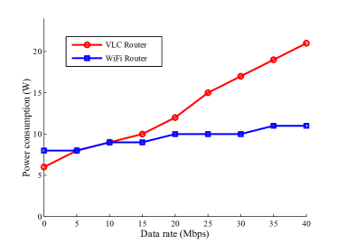
Figure 1: Preliminary experimental results of power consumption vs. throughput for VLC and WiFi data transmissions

If different users connecting to the same AP use different channels, the power additive model is applied. In this model, except for the power to turn-on the AP, the additional power needed to serve a user at a given location, a given field of view (FOV), and a given data rate by a given AP is fixed regardless of the number of users served by the same AP. Even when assigning different users to one channel, our preliminary experimental results have validated the suitability of the power additive model for VLC in an indoor environment. As shown in Fig. 1. The VLC and WiFi power consumption measurements are performed based on our VLC front-ends and a NETGEAR Wireless Dual Band Gigabit Router WNDR4500, respectively. VLC and WiFi transmitters are set to keep sending UDP packets at different data rates while a power meter is attached to the transmitters to monitor the power consumption. The power consumptions for both VLC and WiFi are approximately proportional to the data rate when the turn-on power is not considered, which validates the suitability of the power additive model for both wireless access technologies. Other experimental studies for WiFi also validate this model [46, 47, 48, 49].

Let the $m$-th AP be a VLC AP; we use $P_{m}^{on}$ to denote the electrical power consumed when the whole transmitted optical power from the $m$-th AP is generated by DC current. If the $m$-th AP is only used to provide illumination, $P_{m}^{on}$ will represent the total consumed power at that AP. We use $P_{mn}$ to denote the extra electrical power (i.e. caused by AC current switching loss) consumed to support a data rate of $R_{n}$ for the $n$-th user through the $m$-th AP. Based on the power additive model, knowing both $P_{m}^{on}$ and $P_{mn}$, the power consumption of a VLC AP when performing joint communications and illumination can be fully characterized. Note that $P_{m}^{on}$ depends on the required illumination level. Therefore, $P_{mn}$ needs to be fully characterized when the $n$-th user initiates the request to be served. For stationary users, the VLC channel is very stable as compared to the RF channel [50]. Therefore, the channel state information (CSI) in terms of signal-to-noise ratio (SNR) or bit error rate (BER) is able to provide a good estimation for these values.

II-E RF Device-Level Model

If the $m$-th AP is an RF AP, its total power consumption can be written as $P^{on}_{m}+\sum_{n\in\mathcal{N}(m)}P_{mn}.$ Here, $P^{on}_{m}$ is the power needed to turn on the RF AP, $P_{mn}$ is the extra power required to support a data rate of $R_{n}$ to the $n$-th user from the $m$-th AP and $\mathcal{N}(m)$ is the set of users that are connected to the $m$-th AP. As explained in [51, 52], $P^{on}_{m}$ represents the major component of the power consumption of the WiFi or the femtocell AP. Here, the power additive model is utilized, which is validated by preliminary experimental results and by [46, 47, 48, 49]. $P_{m}^{max}$ is used to represent the maximum $(\sum P_{mn})$ that the AP can support. If the $m$-th AP is an RF one, both $P_{m}^{on}$ and $P_{m}^{max}$ will be fixed. On the other hand, $P_{m}^{max}$ depends on $P_{m}^{on}$ for the VLC AP, which could be fixed or could be controllable depending on the ambient illumination level that is changing over time.

When the ambient light level is very small, $P_{m}^{on}$ for the VLC APs will be utilized for lighting, thus making the VLC AP power-proportional, i.e., the total power consumed by the VLC AP for communications is proportional to the data rate. Designing a power proportional communications device is considered ideal rather than realistic to be achieved [53, 54, 55]. Here, it is shown that jointly performing illumination and communications can potentially realize the power proportional AP. On the other hand, when the ambient light level is large, $P_{m}^{on}$ will either be very small so that it cannot support high data rates or be large to support high data rates but not to be utilized for lighting. This makes the VLC AP power non-proportional in this case.

III Problem Formulation

III-A Hybrid WiFi-VLC System Problem Formulation

The problem of minimizing the total power consumption is formulated as the following Mixed Integer Linear Program (MILP):

$$\mathbb{P}1:\min\sum_{m=1}^{M}P_{m}^{on}X_{m}+\sum_{m=1}^{M}\sum_{n=1}^{N}P_{mn}Y_{mn}$$ (1)

subject to

$$Y_{mn}\leq X_{m},\quad\forall n,m$$ (2)

$$\sum_{m=1}^{M}Y_{mn}\geq 1\quad\forall n$$ (3)

$$\sum_{n=1}^{N}P_{mn}Y_{mn}\leq X_{m}P_{m}^{max}\quad\forall m$$ (4)

$$\sum_{m\in VLC}\bigl{[}(\frac{g+1}{2\pi})\frac{\cos^{g}(\theta_{m})\cos(\psi_{m})}{r_{mw}^{2}}G_{m}P_{m}^{on}\eta_{m}^{DC}X_{m}\bigr{]}\geq\mathcal{I}_{w}$$ (5)

Here, $X_{m}=\left\{\begin{array}[]{rl}1&\mbox{if the $m$-th AP is on}\\ 0&\mbox{otherwise.}\end{array}\right.$

$Y_{mn}=\left\{\begin{array}[]{rl}1&\mbox{if the $n$-th user is connected to the}\\ &\mbox{$m$-th AP}\\ 0&\mbox{otherwise.}\end{array}\right.$

We assume that the output optical power of a VLC AP is fixed. Therefore, in the objective function of the stated problem formulation, the first term refers to the total power consumption for turning on the APs while the second term refers to the total power consumption for data transmission. The first set of constraints ensures that a user cannot connect to an AP that is not turned on. The second set of constraints ensures that a user should be connected to at least one AP. The third set of constraints ensures that the total power consumed by an AP does not exceed its maximum power consumption limit. The last set of constraints is the illumination constraints. Here, $\mathcal{I}_{w}$ represents the illumination level required at the $w$-th location. Note that the value of $\mathcal{I}_{w}$ can be zero if the ambient light is suffient. If illumination is not required, a VLC AP might still be turned on to reduce the total power consumption. Regarding the issue about turning on VLC APs while illumination is not required, we discuss it in three cases. 1) Illumination is not needed but turning on VLC APs is acceptable. Case 1 is the situation studied in our simulation settings (Sec. VI). Turning on VLC APs at day especially for communication purpose is capable of reducing the total power consumption and the additional illumination produced by VLC APs will not cause the illumination levels exceeding the recommended range. 2) Illumination is not needed and turning on VLC APs will produce unexpected brightness. Case 2 considers scenarios when darkness is preferred. For case 2, maximum illumination constraints can be added to the optimization problem and different maximum illumination levels will lead to different results. Case 2 will be studied in the future. 3) Illumination is not needed but turning on VLC APs will not produce unexpected brightness. In case 3, turning on VLC APs for communication may not produce any human-sensitive lighting. [56] presents the approach that enables a VLC AP for communication while keep the environment being dark. The main idea is utilizing pulse width modulation for VLC and reducing the pulse width in each symbol to perform the brightness control. The method proposed in [56] provides a flexible solution to case 2 where the maximum illumination constraint varies. If the $m$-th AP is a VLC one and it is sending only DC signal, we use $\eta_{m}^{DC}$ to represent its efficiency. Note that the output optical power of a VLC AP is fixed. Therefore, $P_{m}^{op}=P_{m}^{on}\eta_{m}^{DC}$. In the following, we show that our problem is NP-complete.

III-B NP-Completeness Proof

The following theorem shows that our problem is NP-complete.

Theorem 1.

The ILP optimization problem is NP-complete.

Proof.

Given any solution to our problem, we can easily check the solution’s feasibility in polynomial time by checking the constraints. Since the number of constraints is polynomial in terms of the number of users, APs, and locations, our problem belongs to NP.

To prove that our problem is NP-hard, we reduce the capacitated facility location problem, which is known to be an NP-complete problem, to an instance of our problem. The capacitated facility location problem is defined as follows: Given a set of facilities $I$ and a set of users $D$, we wish to open a subset of facilites to serve the users in $D$, where each facility $i\in I$ has an opening cost $q_{i}$, a capacity $c_{i}$, and the cost of serving a user $d$ from a facility $i$ is $r_{id}$. The objective is to minimize the total cost.

The reduction is performed as follows: (1) The $i$-th facility in the facility location problem is mapped to the $m$-th AP in our problem. (2) The $d$-th user in the facility location problem is mapped to the $n$-th user in our problem. (3) $P_{m}^{on}=q_{i}$, (4) $P_{m}^{max}=c_{i}$. (5) $P_{mn}=r_{id}$. (6)$\mathcal{I}_{w}=0,\forall w$.

Now we prove that there exists a solution to the capacitated facility location problem with cost $\mathcal{A}$ if and only if there exists a solution to our problem with cost $\mathcal{A}$.

If there exists a solution to the capacitated facility location problem with cost $\mathcal{A}$, then the set of opened facilities represents the APs that are turned on, a facility $i$ serving user $d$ represents the $m$-th AP serving the $n$-th user, and the total cost of our problem is $\mathcal{A}$. The proof of the other direction of the if and only if statement is done in a similar way. ∎

IV Online Algorithm

To solve the offline optimization problem $\mathbb{P}1$, one can use an optimizer such as CPLEX [57]. Solving $\mathbb{P}1$ requires the knowledge of all requests for connections from users apriori. However, such knowledge is not available in real scenarios. Alternatively, one can recompute the solution to $\mathbb{P}1$ whenever a new request (or batch of requests) for connection from a user (users) appears, but this may lead to the reconfiguration of the system with the appearance of the request and may require advanced techniques, such as soft handover, to avoid connection disruption for previous users when switched to a different AP. Moreover, recomputing the solution to $\mathbb{P}1$ will lead to additional intolerable delays to the new user since the complexity of resolving $\mathbb{P}1$ increases as the number of users increases. Therefore, we present in this section a randomized online algorithm for the hybrid RF-VLC system, to tackle the above-mentioned issues.

In the online version of the problem addressed here, requests for connections from users appear one by one. The online algorithm has to make a decision to connect the user to an AP, and the algorithm’s decision has to be made before the next user appears. Moreover, the decisions of the online algorithm cannot be reversed in the future. Due to the NP-completeness of the problem as shown in Theorem 1, we remove the $P_{m}^{max}$ constraint and assume that there is no limit on it. In the simulation results, we show that the power consumption of the online algorithm is not high (in order of 50 Watts for 100 users)

To compare the performance of the online algorithm to that of the optimal offline algorithm, we use the concept of competitive ratio. The competitive ratio is defined as the worst-case ratio of the performance achieved by the online algorithm to the performance achieved by the optimal offline algorithm, i.e., if we denote the performance of the online algorithm by $\mathcal{P}_{on}$ and that of the optimal offline algorithm by $\mathcal{P}_{off}$, then the competitive ratio is:

$$\sup_{All\ requests}\frac{\mathcal{P}_{on}}{\mathcal{P}_{off}}.$$

To experimentally measure the competitive ratio, one needs to find the input sequence (among $2^{M}$ possible input sequences) that gives the worst possible performance, which becomes infeasible as $M$ grows large. As the ratio gets closer to 1, the online performance gets closer to the offline performance. In other words, the smaller the competitive ratio is, the better the online algorithm’s performance will be.

In the online algorithm, we may desire to satisfy the illumination requirements before the appearance of any request for connection from users. Therefore, we decompose the optimization problem $\mathbb{P}1$ into two subproblems. In the first subproblem, we solve an optimization problem to find the set $\mathcal{M}^{\prime}$ of turned-on VLC APs to satisfy the illumination requirements, and is formulated as follows:

$$\mathbb{P}2:\min\sum_{m\in VLC}P_{m}^{on}X_{m}$$ (6)

subject to

$$\sum_{m\in VLC}\bigl{[}(\frac{g+1}{2\pi})\frac{\cos^{g}(\theta_{m})\cos(\psi_{m})}{r_{mw}^{2}}G_{m}P_{m}^{on}\eta_{m}^{DC}X_{m}\bigr{]}\geq\mathcal{I}_{w}$$ (7)

Given the set of turned-on VLC APs, the second subproblem is to minimize the power consumption by all APs while satisfying the users’ requests, and is formulated as follows:

$$\mathbb{P}3:\min\sum_{m=1}^{M}P_{m}^{on}X_{m}+\sum_{m=1}^{M}\sum_{n=1}^{N}P_{mn}Y_{mn}$$ (8)

subject to

$$X_{m}=1,\quad\forall m\in\mathcal{M}^{\prime}$$ (9)

$$Y_{mn}\leq X_{m},\quad\forall n,m$$ (10)

$$\sum_{m=1}^{M}Y_{mn}\geq 1\quad\forall n$$ (11)

$$\sum_{n=1}^{N}P_{mn}Y_{mn}\leq X_{m}P_{m}^{max}\quad\forall m$$ (12)

Note that the two subproblems are also NP-complete, which can be proved by a reduction from the facility location problem as illustrated in Section III-B. Our online algorithm proposed here for problem $\mathbb{P}3$ is inspired by the idea of the online algorithm presented in [58]. We construct a graph $G=(V,E)$ consisting of $M+N+1$ vertices, where $M$ is the number of APs, $N$ is the number of users, and the additional vertex represents a virtual source $S$, which could represent the gateway router and the centralized controller that all APs are connected to. We connect the source $S$ to each of the $M$ APs, and each AP to all of the users that the AP can serve. We associate two values for each edge $e$. The first value represents the flow on the edge $w_{e}$ and is unitless. The weights are dynamically changing during the run of the algorithm and their values are in the range [0, 1]. The second value associated with an edge is the edge’s cost $c_{e}$, which represents the power consumption of that edge and has the unit of Watts. There are three types of edges when assigning these initial costs:

• The first type of edges is an edge connecting the virtual source $S$ to a VLC AP that is already turned on to satisfy illumination requirements (as determined from solving the optimization problem $\mathbb{P}2$). The set of turned-on APs due to solving $\mathbb{P}2$ is represented by $\mathcal{M}^{\prime}$. The initial cost of an edge connecting the virtual source $S$ to an AP $m\in\mathcal{M}^{\prime}$ is set to 0.

• The second type of edges contains the edges connecting the virtual source to the remaining APs (i.e., the VLC APs that are not in the set $\mathcal{M}^{\prime}$ and WiFi APs). The initial cost of an edge connecting the virtual source $S$ to an AP $m\notin\mathcal{M}^{\prime}$ is set to the power consumption ($P_{m}^{on}$) required to turn on the $m$-th AP.

• The third type of edges is an edge connecting a user to an AP. The initial cost of an edge connecting the $n$-th user to the $m$-th AP is set to the power consumption ($P_{mn}$) required if the $n$-th user is to be connected to the $m$-th AP.

For example, as shown in Fig. 2, the cost of the edge connecting $AP1$ to user 1 in the graph on the right side of the figure is set to $P_{11}$, which is the power consumed if user 1 is to be connected to $AP1$ in our problem (the graph on the left side of Fig. 2).

After the graph is constructed, our problem becomes equivalent to the following Minimum Cost Connectivity (MCC) problem on the newly constructed graph:

$${\color[rgb]{0,0,0}\mathbb{P}4:}\min\sum_{e}w_{e}c_{e}$$

subject to

$$max\_flow(S,n,w)\geq 1\quad\forall n$$ (13)

where $c_{e}$ is the cost of edge $e$, $w_{e}$ is the weight of edge $e$, and $max\_flow(S,n,w)$ is the maximum flow from the source $S$ to the $n$-th user when the capacity of each edge is 1 and the flow on each edge is represented by the weight [59]. The Minimum Cost Connectivity (MCC) problem is defined as follows: given a graph $G^{\prime}=(V^{\prime},E^{\prime})$ with cost function $c:E^{\prime}\rightarrow\mathbb{R}^{+}$, and a demand $D_{i}=(s_{i},t_{i})$, where $s_{i}$ is the source of $D_{i}$ and $t_{i}$ is the sink of $D_{i}$. The objective is to find an assignment of weights $w\in\{0,1\}$ to $E^{\prime}$, such that there is a flow from $s_{i}$ to $t_{i}$ of value at least 1 with the minimum cost, where the cost is equal to $\sum_{e\in E^{\prime}}w_{e}c_{e}$. Constraint 13 states that the flow from the source to each user must be at least 1 in order to satisfy the user’s demand. An example of the reduction with the cost assigned to the edges is shown in Fig. 2, which shows how our problem can be mapped to the new problem $\mathbb{P}4$. Since the costs of the edges in the graph represent the power consumption of turning on an AP or connecting a user to an AP, a solution that minimizes the total cost in problem $\mathbb{P}4$ while having a flow of value of at least 1 from the virtual source $S$ to every destination is a solution that minimizes the power consumption in our problem $\mathbb{P}3$ while satisfying the users’ demands.

Figure 2: Constructing the graph for the online algorithm.

The online algorithm is described in Algorithm 1 and the notations used in the algorithm are presented in Table I. The algorithm operates in an online fashion upon each user’s arrival. The algorithm consists of two phases. In the first phase, the algorithm computes a fractional solution. The second phase is a randomized rounding phase, where the algorithm rounds the fractional solution computed in the first phase to an integral solution.

TABLE I: Notations used in Algorithm 1

Notation	Definition
$\alpha$	Guess of the value of the optimal fractional solution
$c_{e}$	Cost of edge $e$
$c_{e}^{{}^{\prime}}$	Normalized version of $c_{e}$
$c_{tot}^{frac}$	Total fractional cost of the online algorithm
$c_{tot}$	Total integral cost of the solution of the online algorithm
$w_{e}$	Weight of edge $e$
$w_{e}^{{}^{\prime}}$	Weight of edge $e$ updated by the online algorithm
$\gamma_{e}$	Value of the threshold associated with edge $e$
$\mathcal{C}$	Minimum weight cut
$\Gamma(e,j)$	Set of random variables associated with edge $e$

1:  Solve the ILP Optimization Problem (6) using CPLEX to find the set of turned-on VLC APs, $\mathcal{M}^{\prime}$.

2:  $\forall e$ connecting $S$ to $m,m\in\mathcal{M}^{\prime}$, $c_{e}=0$

3:  $\forall e$ connecting $S$ to $m,m\notin\mathcal{M}^{\prime}$, $c_{e}=P_{m}^{on}$

4:  $n^{\prime}=0$

5:  $\alpha=\min_{e}c_{e}\quad|e\text{\leavevmode\nobreak\ connecting\leavevmode\nobreak\ }S\text{\leavevmode\nobreak\ to\leavevmode\nobreak\ }m,m\notin\mathcal{M}^{\prime}$

6:  $w_{e}=w_{e}^{{}^{\prime}}=\frac{1}{M^{2}}$

7:  $c_{tot}=0$

8:  Upon the arrival of a new user $u$

9:  $n^{\prime}\leftarrow n^{\prime}+1$

10:  $\forall e$ connecting $m$-th AP to $u$, $c_{e}=P_{mu}$

11:  $\forall e$, keep $\lceil 2\log(n^{\prime}+1)\rceil$ independent random variables $\Gamma(e,j)$, $1\leq j\leq\lceil 2\log(n^{\prime}+1)\rceil$, uniformly distributed in the interval [0, 1]. Define a threshold $\gamma_{e}=\min_{j}\Gamma(e,j)$ (for randomized rounding)

12:  START:

13:  $\forall e$ such that $c_{e}\leq\frac{\alpha}{M}$, set $w_{e}=w_{e}^{{}^{\prime}}=1$

14:  $\forall e$ such that $\frac{\alpha}{M}\leq c_{e}\leq\alpha$, set $c_{e}^{{}^{\prime}}=\frac{c_{e}}{\alpha/M}$

15:  if the maximum flow between $S$ and $u$ is at least 1 (i.e., user is already satisfied) then

16:     do nothing

17:  else

18:     while the flow is less than 1 (i.e., user is not satisfied yet) do

19:        Compute the minimum weight cut $\mathcal{C}$ between $S$ and $u$

20:        $\forall e\in\mathcal{C}$, $w_{e}^{{}^{\prime}}\leftarrow w_{e}^{{}^{\prime}}(1+\frac{1}{c_{e}^{{}^{\prime}}})$ (, weight augmentation step)

21:  $w_{e}=\max\{w_{e},w_{e}^{{}^{\prime}}\}$

22:  $c_{tot}^{frac}=\sum_{e}w_{e}c_{e}^{{}^{\prime}}$

23:  if $w_{e}\geq\gamma_{e}$ (Randomized Rounding) then

24:     $w_{e}=1$

25:  else

26:     $w_{e}=0$

27:  $c_{tot}=\sum_{e}w_{e}c_{e}^{{}^{\prime}}$

28:  if $c_{tot}^{frac}>2\alpha\log(M)+\alpha+1$ then

29:     $\alpha\leftarrow 2\alpha$

30:     Go to START

Algorithm 1 Online Hybrid RF-VLC System

For the first phase, the algorithm uses the doubling technique to guess the value of the optimal fractional solution denoted by $\alpha$. To get the intuition of the doubling technique, suppose that the online algorithm has a competitive ratio of $\Theta$ and the true cost of the optimal solution is $c^{*}$. We begin with the initial guess of the optimal cost $\alpha$, and run the algorithm assuming this guess is the correct estimate of $c^{*}$. If the online algorithm fails to find a feasible solution of a cost at most $\Theta\alpha$, we double the value of $\alpha$ and continue with the algorithm. Eventually, $\alpha$ will exceed $c^{*}$ by at most a factor of 2, and for this value of $\alpha$, the algorithm will compute a feasible solution (since all demands are satisfied as shown in Section V) of cost at most $2\Theta c^{*}$. Therefore, we can assume that the value of the optimal solution is known.

The initial guess of $\alpha$ is set to $\alpha=\min_{e}c_{e}$. Based on the value of $\alpha$, we sort the edges into three categories. The first category includes all edges with a cost less than $\frac{\alpha}{M}$. All edges in the first category are assigned a weight of 1, paying at most an additional cost of $\sum_{e\in\mathcal{M}^{\prime}}\frac{\alpha}{M}=\alpha$. The second category includes all edges with a cost greater than $\alpha$. All edges in the second category are excluded from the solution. The third category includes all the remaining edges where $\frac{\alpha}{M}\leq c_{e}\leq\alpha$. All edges in the third category are assigned an initial weight of $\frac{1}{M^{2}}$ and their costs are normalized by $\frac{\alpha}{M}$ to be between $1$ and $M$. The algorithm then updates the weights of the edges in the third category until the minimum weighted cut is greater than 1. During the execution of the algorithm, it may turn out that a demand cannot be satisfied (due to the excluded edges from the second category mentioned above), or that the true value of the optimal solution is greater than the current value of $\alpha$ (which can be verified by checking if the cost of the fractional solution exceeds an upper bound on the cost of the algorithm, which is $2\alpha\log(M)+\alpha+1$, known through the competitive-ratio analysis of the algorithm (Theorem 2). In this case, we double the value of $\alpha$, which means that more edges are available for the online algorithm to satisfy the demands, “forget” about the weights assigned to the edges so far, double the value of $\alpha$, and continue the algorithm. Although we “forget” about the weights when $\alpha$ is doubled, the actual weight of an edge used to calculate the total cost of the algorithm is the maximum weight assigned to that edge so far. This ensures that the edges previously chosen will not be unselected over the iterations. If the total cost of the online algorithm is less than $2\alpha\log(M)+\alpha+1$, then we are guaranteed that we achieve a fractional solution that is within a $\log(M)$ factor of $\alpha$.

After the fractional solution is obtained, the algorithm rounds the solution to an integral solution which is within a $\log(N)$ factor of the fractional solution. This is done by comparing the weight $w_{e}$ of an edge $e$ to the threshold $\gamma_{e}$ (as computed in line 11 of Algorithm 1) assigned to that edge. If the weight of the edge is greater than the value of the threshold (line 23 of Algorithm 1), the weight of the edge is set to 1. This randomized rounding process introduces a $\mathcal{O}(\log(N))$ factor to the competitive ratio. Therefore, the competitive ratio of our algorithm is $\mathcal{O}(\log(M)\log(N))$.

The complexity of the online algorithm mainly comes from two parts. The first part is solving the ILP optimization problem in line 1 of Algorithm 1. We note that this optimization problem is only solved once before the arrival of users’ requests. The solution to the problem can be saved for future reference when the same illumination requirements occur again. Moreover, this ILP problem only considers illumination requirements, it has a lower complexity than the original problem $\mathbb{P}1$. The second part is finding the minimum weight cut for every unsatisfied user. There are many algorithms that can find the minimum weight cut in polynomial time [60]. Therefore, the rest of the algorithm has a polynomial time complexity.

V Performance Analysis

In this section, we prove that the competitive ratio of the online algorithm is $\mathcal{O}(\log(M)\log(N))$ with respect to Problem $\mathbb{P}4$. Moreover, we prove that the best competitive ratio achieved by any online algorithm under our settings is $\Omega(\log(M))$. The adversary model used in the proof is an oblivious one. We note that the optimization problem (6) is solved using CPLEX [61] at the beginning of the online algorithm. Therefore, the following proof is for lines 8-28 in Algorithm 1. Since $\alpha$ is the guess of the optimal solution, which is assumed to be known through the doubling technique, $\alpha=\sum_{e}c_{e}^{{}^{\prime}}w_{e}^{*}$, where $w_{e}^{*}$ denotes the weight assigned to edge $e$ by the optimal solution. All logarithms are to the base 2.

Theorem 2.

For a fixed $\alpha$, the online algorithm produces an integral solution that is:

• $\mathcal{O}(\log(M)\log(N))$ competitive.

• The solution is feasible with probability $1-\frac{1}{N}$.

Proof.

Proof.

We first show that the fractional solution of the online algorithm is within a $\mathcal{O}(\log(M))$ factor of the optimal offline solution. Then, we show that the integral solution of the online algorithm is within a $\mathcal{O}(\log(N))$ factor of the fractional solution. Therefore, the integral solution is within an $\mathcal{O}(\log(M)\log(N))$ factor of the optimal offline solution.

We prove that the fractional solution of the online algorithm is within $\mathcal{O}(\log(M))$ of the optimal solution by proving the following two claims:

• The number of weight augmentation steps of the online algorithm is $\mathcal{O}(\alpha\log(M))$.

• In each weight augmentation step, the increment of the total cost of the solution returned by the online algorithm does not exceed 1.

To prove the first claim, consider the following potential function:

$$\beta=\sum_{e}c_{e}^{{}^{\prime}}w_{e}^{*}\log(w_{e}^{{}^{\prime}})$$

where $w_{e}^{*}$ is the weight of edge $e$ computed by the optimal solution, $c_{e}^{{}^{\prime}}$ is the normalized version of the cost $c_{e}$ of edge $e$ as computed in line 14 of Algorithm 1 and $w_{e}^{{}^{\prime}}$ is the weight of edge $e$ updated by the online algorithm. We show that if the potential function is updated after each weight augmentation step, then we have the following properties of the potential function:

• Initially, $\beta=-2\alpha\log(M)$.

• When the algorithm terminates, $\beta\leq\alpha$.

• In each weight augmentation step, $\Delta\beta\geq 1$.

These properties guarantee that the number of weight augmentation steps performed by the online algorithm is at most $\alpha+2\alpha\log(M){\color[rgb]{0,0,0}+1}=\mathcal{O}\log(M)$. To prove the first property, note that initially, $w_{e}^{{}^{\prime}}=\frac{1}{M^{2}}$ and $\beta=\sum_{e}c_{e}^{{}^{\prime}}w_{e}^{*}\log(\frac{1}{M^{2}})=-2\alpha\log(M)$. To prove the second property, the weight of each link is at most 2 when the algorithm terminates, and $\beta\leq\sum_{e}c_{e}^{{}^{\prime}}w_{e}^{*}\log(2)=\alpha$. To prove the third property, note that in each augmentation step, we have:

$$\Delta\beta =\sum_{e\in\mathcal{C}}c_{e}^{{}^{\prime}}w_{e}^{*}\log(w_{e}^{{}^{\prime}}(1+\frac{1}{c_{e}^{{}^{\prime}}}))-\sum_{e\in\mathcal{C}}c_{e}^{{}^{\prime}}w_{e}^{*}\log(w_{e}^{{}^{\prime}})$$

$$=\sum_{e\in\mathcal{C}}c_{e}^{{}^{\prime}}w_{e}^{*}\log(1+\frac{1}{c_{e}^{{}^{\prime}}})\geq\sum_{e\in\mathcal{C}}w_{e}^{*}\geq 1$$

where the last inequality follows from the fact that the total weight assigned by the optimal solution to the edges in the cut is at least 1. Therefore, the number of weight augmentation steps performed by the online algorithm is at most $2\alpha\log(M)+\alpha+1=\mathcal{O}(\alpha\log(M))$.

To prove the second claim, consider an iteration in which a new user arrives and the weight augmentation step is performed. The total weight of the links in $\mathcal{C}$ is less than 1, and the weight of each link $e\in\mathcal{C}$ will increase by $w_{e}^{{}^{\prime}}c_{e}^{{}^{\prime}}$. Therefore, the total increase of the cost of the solution returned by the online algorithm in a single weight augmentation step is:

$$\sum_{e\in\mathcal{C}}\frac{w_{e}^{{}^{\prime}}}{c_{e}^{{}^{\prime}}}c_{e}^{{}^{\prime}}=\sum_{e\in\mathcal{C}}w_{e}^{{}^{\prime}}\leq 1$$

From the first claim, the total number of weight augmentation steps is $\mathcal{O}(\alpha\log(M))$. Therefore, the fractional solution of the online algorithm is within a $\log(M)$ factor of the optimal solution.

Figure 3: The system used in the proof of Theorem 3.

The proof that the integral solution of the online algorithm is within $\mathcal{O}(\log(N))$ of the fractional solution, and is feasible with probability $1-\frac{1}{N}$ is explained as follows.

For each $j,1\leq j\leq 2\log(N+1)$, the probability that $\Gamma(e,j)\leq{\color[rgb]{0,0,0}w_{e}}$ is exactly ${\color[rgb]{0,0,0}w_{e}}$. Let $Z$ denote the set of edges whose weights are set to 1 after the rounding process. Note that the probability that an edge $e\in{\color[rgb]{0,0,0}Z}$ is the probability that there exists a $j$ such that $\Gamma(e,j)\leq{\color[rgb]{0,0,0}w_{e}}$. Let $Y(e,j)$ denote the indicator of the event that $\Gamma(e,j)\leq{\color[rgb]{0,0,0}w_{e}}$ (i.e., $Y(e,j)=1$ if $\Gamma(e,j)\leq{\color[rgb]{0,0,0}w_{e}}$, and 0 otherwise). Since $\Gamma(e,j)$ is chosen uniformly at random in the range [0, 1], the probability and the expectation of the indicator $Y(e,j)$ is at most ${\color[rgb]{0,0,0}w_{e}}$. Therefore, the expected cost of the integral solution is

$$\mathbb{E}\bigl{[}\sum_{e\in{\color[rgb]{0,0,0}Z}}c_{e}\bigr{]} \leq\sum_{e\in E}\sum_{j=1}^{2\log(N+1)}c_{e}\mathbb{E}[Y(e,j)]$$

$$\leq\sum_{e\in E}\sum_{j=1}^{2\log(N+1)}c_{e}{\color[rgb]{0,0,0}w_{e}}=2\log(N+1)\sum_{e\in E}c_{e}{\color[rgb]{0,0,0}w_{e}}$$

Therefore, the expected cost of the integral solution is at most $2\log(N+1)$ times the cost of the fractional solution.

To prove that the solution is feasible with probability $1-\frac{1}{N}$, pick any user $n$. The probability that user $n$ is not served is the probability that all of the edges connecting the virtual source $S$ to user $n$ has $\Gamma(e,j)>{\color[rgb]{0,0,0}w_{e}},\forall j,1\leq j\leq 2\log(N+1)$. This probability is:

$$\prod_{j}\prod_{e}(1-Y(e,j)) =\prod_{j}\prod_{e}(1-{\color[rgb]{0,0,0}w_{e}})$$

$$\leq\prod_{j}\exp(-\sum_{e}{\color[rgb]{0,0,0}w_{e}})$$

$$\leq\prod_{j}exp(-1)=\exp(-2\log(N+1))$$

$$\leq\frac{1}{N^{2}}$$

The first inequality follows since $(1-{\color[rgb]{0,0,0}w_{e}})\leq\exp(-{\color[rgb]{0,0,0}w_{e}})$. The second inequality follows since user $n$ is satisfied in the fractional solution and thus $\sum_{e}w_{e}\geq 1$. Using the union bound, the probability that there exists an unserved user in the integral solution is at most $N\frac{1}{N^{2}}=\frac{1}{N}$. ∎

∎

Note that the process of doubling $\alpha$ results in an additional factor of 2 of the competitive ratio, and “forgetting” the weights when $\alpha$ is doubled results in an additional factor of 2, to a total additional factor of 4. Nevertheless, the competitive ratio of the online algorithm is $\mathcal{O}(\log(M)\log(N))$.

Now we prove a lower bound on the competitive ratio achieved by any online algorithm by proving the following theorem:

Theorem 3.

The best competitive ratio achieved by any online algorithm is $\Omega(\log(M))$.

Proof.

To prove this theorem, we provide an example network such that any online algorithm implemented over this network cannot achieve a competitive ratio better than $\Omega(\log(M))$. Consider a system with $M$ APs and $\log(M)$ users. The first user is connected to all APs, the second user is connected to the first $\frac{M}{2}$ APs, the $n$-th user is connected to the first $\frac{M}{2^{n-1}}$. The system has the following properties:

• The power consumption required to turn on an AP is the same for all APs and is equal to $f$.

• The power consumption required for data transmission between a user and an AP is equal to 0 if the user is connected to the AP, and is otherwise equal to infinity.

The system used in the proof is shown in Fig. 3.

In this system, users arrive sequentially and in-order starting from the first user up to the last user. Sequentially means that the online algorithm has to satisfy a user before considering the next one. Consider the $n$-th user. The probability that the $n$-th user is connected to an AP, which was turned on to satisfy the ($n-1$)-th user is, $\frac{1}{2}$. This is because the AP that was turned on due to the ($n-1$)-th user is either connected to both the ($n-1$)-th and $n$-th users, in which case the $n$-th user is satisfied without turning on any additional APs, or the turned on AP is connected to the ($n-1$)-th user but is not connected to the $n$-th user, in which case the $n$-th user is satisfied by turning on an additional AP. Therefore, the total power consumption of the online algorithm is $\sum_{n=1}^{\log(M)}\frac{f}{2}=\frac{f}{2}\log(M)$. The optimal algorithm will turn on a single AP connected to the last user, and so the total power consumption of the optimal algorithm is $f$. Therefore, the best competitive ratio achieved by any online algorithm is $\Omega(\log(M))$. ∎

VI Numerical Results

In this section, we present the simulation results for the following schemes:

• Hybrid: our optimal hybrid scheme.

• VLC: in this scheme, communications is performed using the VLC APs only and the same optimization problem considered for the hybrid scheme is performed but only on the VLC APs.

• WiFi: in this scheme, communications is performed using the WiFi APs only and the same optimization problem considered for the hybrid scheme is performed but only on the WiFi APs.

• Online: our proposed online algorithm.

Note that the first three schemes are offline and represented by NP-complete problems. The simulations are conducted using Matlab R2013b. CPLEX 12.6.1 [57] is utilized to run the offline optimization problems.

VI-A Simulation settings

We consider the first floor of the Electrical and Computer Engineering Department building at New Jersey Institute of Technology. The entire storey consists of 16 external rooms, 4 internal rooms, annular corridors and stairways located in corners. Each external room has a lateral window while the internal rooms do not. In the simulations, we assume that user terminals (UTs) are uniformly distributed at random in rooms. There are 4 WiFi APs deployed in corners on the fourth floor. In each room, one light source equipped with 4 VLC APs is mounted on the ceiling. The beamangle (i.e. formed by the central luminous flux and the central vertical line) of each VLC AP is pre-configured in order to position the intersection of the center luminous flux and the horizontal UTs plane at the center of each square region. The benefit of this new light source configuration is manifested in [62]. These system model parameters are summarized in Table II.

TABLE II: System Model Parameters

floor size	18.0 m $\times$ 18.0 m $\times$ 3.0 m
room size	3.0 m $\times$ 3.0 m $\times$ 3.0 m
number of internal rooms	4
number of external rooms	16
height of desk	0.85 m
number of VLC APs	80
number of WiFi APs	4

For a VLC AP, we set $P_{m}^{on}=15$ watts. The wallplug efficiency factors $\eta_{m}^{DC}$ and $\eta_{m}^{AC}$ denote the ratios of emitted optical power to injected electrical power when the $m$-th VLC AP is only sending DC signals and AC signals, respectively. $\eta_{m}^{DC}$ for all the VLC APs is set to 0.1 [63], while $\eta_{m}^{AC}$ is varied to represent different driver circuitry. The channel bandwidth of each VLC AP is 100 MHz. In each room, 4 VLC APs transmit data over 4 different channels, while other 4 VLC APs in a different room can reuse those 4 channels due to the obstacles posed by walls. When multiple UTs are connected to the same VLC AP, they access the same spectrum resource by time division multiplexing (TDM). We assume that, in any fraction of one time slot, a VLC AP is either sending AC signals or DC signals. Thus, the maximum power consumption of a VLC AP $P_{m}^{max}=P_{m}^{on}\times\eta_{m}^{DC}/\eta_{m}^{AC}$. To calculate $P_{mn}$ for the $n$-th UT connected to the $m$-th VLC AP, we start by calculating the VLC link capacity $C_{mn}$ based on Shannon-Hartley theorem [64], assuming the VLC AP is always sending AC signals and the AC signal strength is twice that of the average DC level. Then, the additive power consumed by the $n$-th UT is $\frac{R_{n}}{C_{mn}}\times P_{m}^{on}\times(\frac{\eta_{m}^{DC}}{\eta_{m}^{AC}}-1)$, where $R_{n}$ is the required data rate of the $n$-th UT. The semi-angle at half power of each VLC AP is set to 30^∘. The constant Gaussian noise, dominated by thermal noise, is calculated from the parameters in [45] and set to be 4.7$\times$10^-14 A². The receiver parameters (i.e., FOV of receiver, detector area of a photodiode, gain of optical filter, refractive index of lens and O/E conversion efficiency) are the same as those in [45]. The required illuminance level is above 300 lux and the LED luminosity efficacy is 150 lumen per watt of electricity [65]. These VLC parameters are summarized in Table III.

TABLE III: VLC Parameters

$P_{m}^{on}$ of VLC AP	15 W
semi-angle at half power	30∘
VLC channel bandwidth	100 MHz
constant Gaussian noise	4.7$\times$10-14 A2
detector area of photodiode	1.0 cm2
O/E conversion efficiency	0.54 A/W
gain of optical filter	1.0
refractive index of lens	1.5
FOV of receiver	90 deg.
LED luminosity efficacy	150 lm/W
DC efficiency factor	0.1

For a WiFi AP, we set $P_{m}^{on}=10$ watts [66] and the maximum power consumption of a WiFi AP $P_{m}^{max}=4$ watts for the NETGEAR model WNDR3400v3. Since WiFi APs are deployed on the fourth floor, the WiFi signal strength attenuation due to floors’ obstruction is set to -30 dB [67]. A typical WiFi noise level $N_{0}$ is -90 dBm [68]. When multiple UTs are connected to the same WiFi AP, they access the network simultaneously by frequency division multiplexing (FDM). The WiFi bandwidth $W$ allocated to each UT is set to 2 MHz. To calculate $P_{mn}$ for the $n$-th UT connected to the $m$-th WiFi AP, we start by calculating the received power to satisfy the required data rate $R_{n}$ at the $n$-th user $P_{rx}=N_{0}(2^{\frac{R_{n}}{W}}-1)$. Based on $P_{rx}$, we calculate the transmitted RF power $P_{tx}$ using Friis equation [69]. When the gains of Tx and Rx antennas are set to 1, $P_{tx}=P_{rx}(\frac{4\pi r_{mn}}{\lambda})^{2}$, where $\lambda=0.125$ meters according to the 2.4 GHz carrier frequency. To convert the transmitted RF power to electrical power consumption of the WiFi AP, we divide $P_{tx}$ by an efficiency factor $\eta_{WiFi}$ obtained from [70]. According to Fig. 4(a) in [70], if the RF power level is changed from 1 to 50 mW, the increase in electrical power consumption is about 500 mW. Therefore, we set $\eta_{WiFi}$ to be 0.1. These WiFi parameters are summarized in Table IV.

TABLE IV: WiFi Parameters

$P_{m}^{on}$ of WiFi AP	10 W
WiFi channel bandwidth	2 MHz
Carrier Frequency	2.4 GHz
Maximum power consumption of WiFi AP	14 W
WiFi noise level	-90 dBm
Attenuation due to floors	-30 dB
Efficiency factor	0.1

To evaluate the ambient light level in each room, we utilize the concept of daylight factor (DF) introduced in [71]. In particular, DF$=(E_{i}/E_{o})\times 100\%$, where $E_{i}$ is illuminance due to daylight at a point on the indoors working plane and $E_{o}$ is simultaneous outdoor illuminance on a horizontal plane from an unobstructed hemisphere of overcast sky. In external rooms, DF increases when the evaluated point get closer to the lateral window. While in internal room, DF $=0$ for the entire UTs plane. According to [72], the luminous efficacy of sunlight $\rho=93$ lm/W, where the watt represents optical power. The variation of solar radiation $R_{sun}$ [W/m²] is collected from [73]. Given these parameters, the indoor ambient light level at position $w$ can be estimated by $\mathcal{I}_{ambient}^{w}=\leavevmode\nobreak\$DF${}^{w}\times\rho\times R_{sun}\times 0.01$.

VI-B Simulation Results

We measure the power consumption of all schemes (i.e. Hybrid, VLC, WiFi and Online) when we change the throughput requirement per UT, the number of UTs, and the hour of the day. For different throughput requirements and number of UTs, we simulate the power consumption for day ($R_{sun}=110$ W/m²) and night ($R_{sun}=0$ W/m²). The results are averaged over 100 runs and shown in Fig. 4 to Fig. 8. In different figures, we vary $\eta_{m}^{AC}$ from 0.06 to 0.09, in order to evaluate the performance of the four schemes as the efficiency of the VLC driver circuitry improves. The power consumption we measure here is after subtracting the minimum power consumption required for illumination.

First, from all the figures, we note that the power consumption of the online scheme is at 2-4 times the power consumption of the hybrid scheme, which is within the $\mathcal{O}(\log(N)\log(M))$ factor proved in Section V.

In Fig. 4 and Fig. 5, 100 UTs are distributed uniformly at random. At night (Fig. 4), as all the VLC APs are turned on for illumination, the power consumption for communication of VLC scheme and online scheme is much lower than that of WiFi scheme. Note that the sudden increases of WiFi performance curve (i.e. green curve) are due to the turning-on of additional WiFi APs. The total additive power of VLC scheme is even lower than the power consumption of turning on a WiFi AP, and thus the hybrid scheme performs the same as VLC. As the wallplug efficiency factor for AC signals $\eta_{m}^{AC}$ increases, the power consumption of VLC and hybrid schemes become negligible, and the performance of online scheme is highly enhanced. During the day (Fig. 5), if communications is not needed, half of the VLC APs are turned on for illumination. When the number of UTs is large, it may force most of the VLC APs to be turned on for communications and produce unnecessary illumination. The results in Fig. 5 validate the analysis, manifested as the higher power consumption of VLC scheme compared to that of WiFi. It is worth noticing that, at 2.5 Mbps, an extra WiFi AP needs to be turned on, which leads to the superiority of the hybrid scheme. Since some UTs are located in the square regions such that the corresponding VLC APs have already been turned on for illumination, those UTs will be connected to VLC APs in the hybrid scheme instead of being connected to an extra WiFi AP. In contrast to the results at night, the performance of online scheme during daytime does not change much as the $\eta_{m}^{AC}$ increases. We also note from the figures that the the online scheme consumes half the power compared to WiFi scheme at high throughputs during the night, and consumes 7 to 17 times less power than the VLC scheme during the day.

In Fig. 6 and Fig. 7, the throughput requirement per UT is 6 Mbps. The results are similar to those shown in Fig. 4 and Fig. 5. The only noticeable point is that in Fig. 7, as the number of UTs increases or in other words the uniformity of UTs increases, the probability of a UT located in a square region such that the corresponding VLC AP has not been turned on for illumination increases. Therefore, the power consumption of the VLC scheme increases fast, as the number of UTs increases. We also note from the figures that the power consumption of WiFi can reach 4 times the power consumption of the online scheme during the night, and the power consumption of the VLC scheme can reach 7 times the power consumption of the online scheme during the day.

In Fig. 8, we set the number of UTs to 100 and throughput requirement per UT to 6 Mbps, to evaluate the performance under the crowded environment. It can be seen that, from 6am to 7pm, the WiFi scheme outperforms the VLC scheme due to the large power penalty of turning on VLC APs, and also the hybrid scheme outperforms both WiFi and VLC schemes due to the fact that some UTs are located under the turned-on VLC APs and the total additive power caused by those UTs are less than the power consumption of turning on a WiFi AP. From 7pm to 6am, the power consumption of the VLC scheme is negligible as compared to the WiFi scheme, and thus the performance of the hybrid scheme is the same as that of VLC. The power-saving of the hybrid scheme over WiFi and VLC schemes could be over 90%. When $\eta_{m}^{AC}=0.09$, the online scheme saves around 75% of the power consumption of the WiFi scheme from 6am to 7pm. While from 7pm to 6am, the online scheme consumes slightly more power than the WiFi scheme. However, this additional power consumption is acceptable since the online scheme does not have the knowledge of the future arrivals of UTs while the WiFi scheme does.

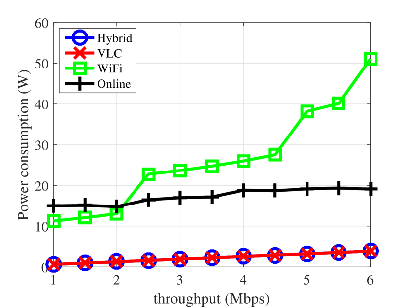
(a) $\eta_{m}^{AC}=0.06$

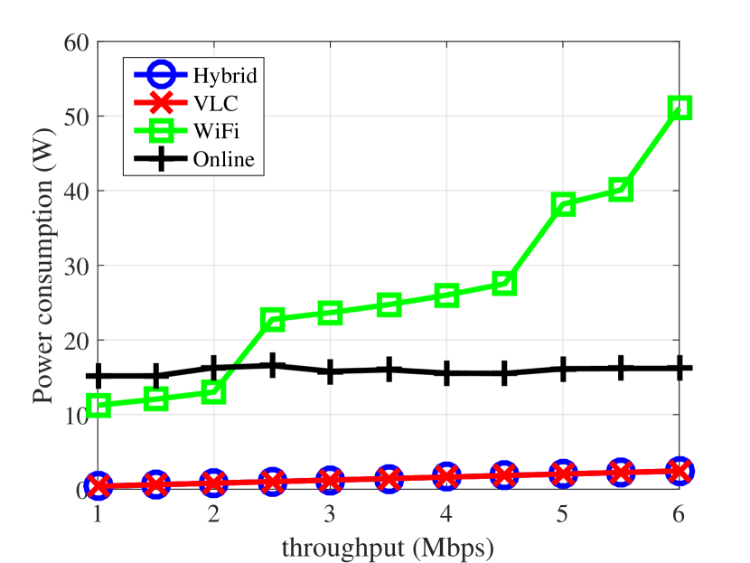
(b) $\eta_{m}^{AC}=0.07$

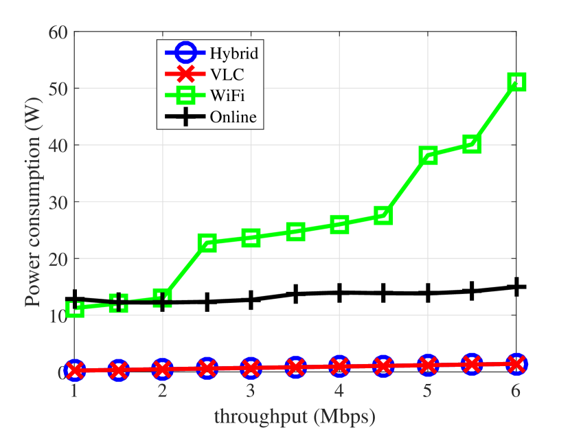
(c) $\eta_{m}^{AC}=0.08$

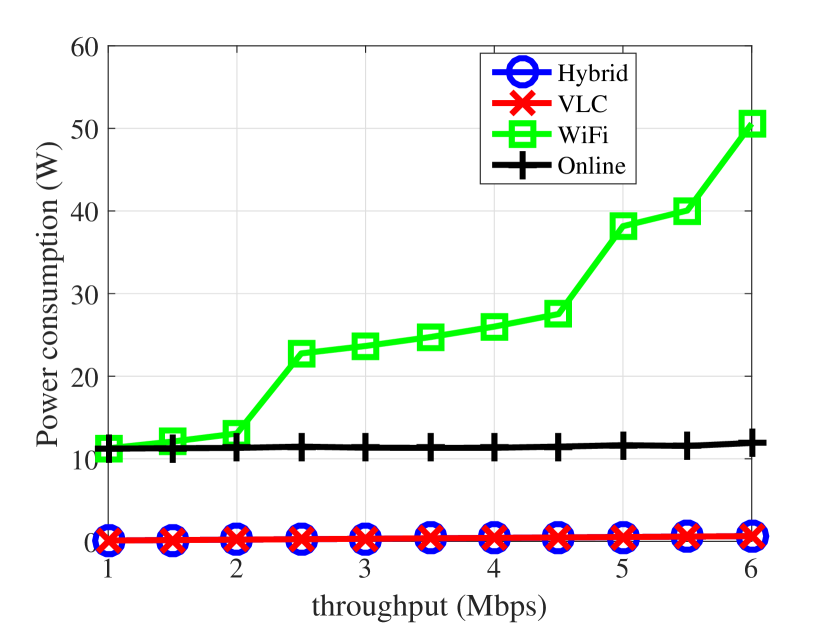
(d) $\eta_{m}^{AC}=0.09$

Figure 4: Power consumption in terms of throughput requirement per user at night

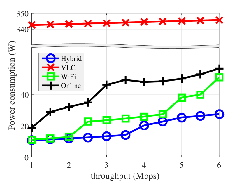
(a) $\eta_{m}^{AC}=0.06$

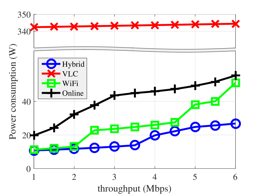
(b) $\eta_{m}^{AC}=0.07$

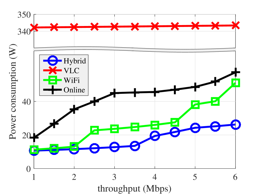
(c) $\eta_{m}^{AC}=0.08$

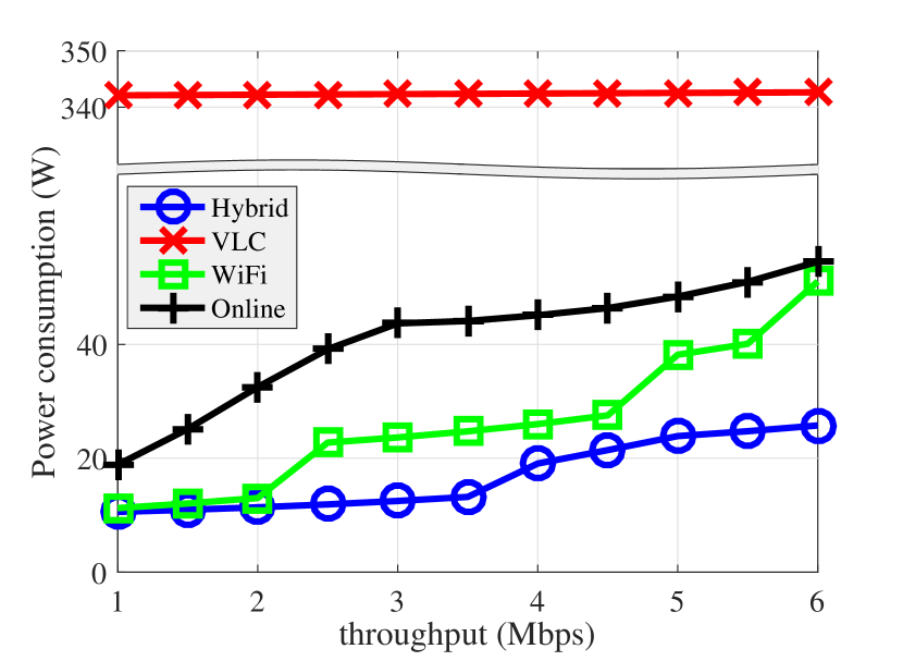
(d) $\eta_{m}^{AC}=0.09$

Figure 5: Power consumption in terms of throughput requirement per user at day

(a) $\eta_{m}^{AC}=0.06$

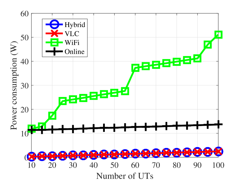
(b) $\eta_{m}^{AC}=0.07$

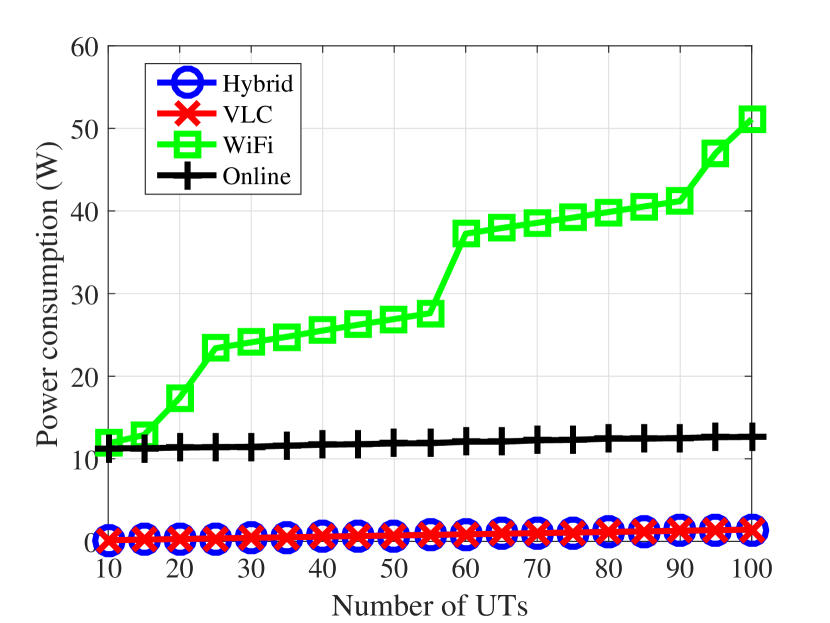
(c) $\eta_{m}^{AC}=0.08$

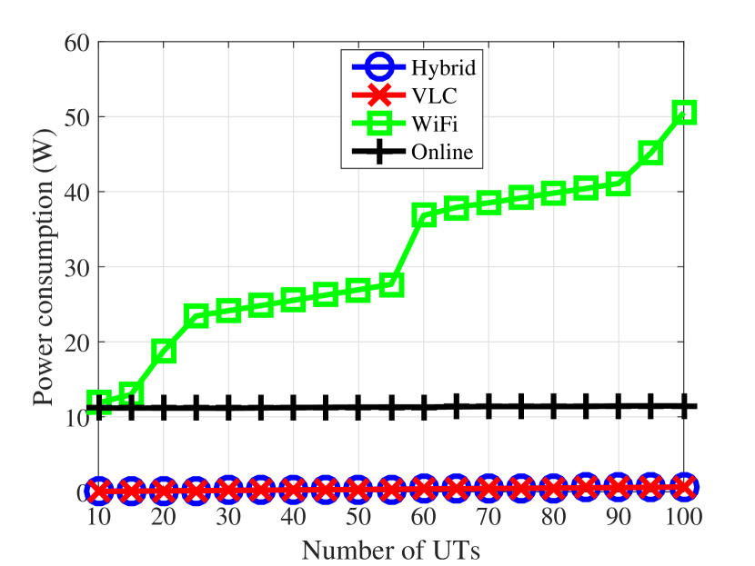
(d) $\eta_{m}^{AC}=0.09$

Figure 6: Power consumption in terms of number of UTs at night

(a) $\eta_{m}^{AC}=0.06$

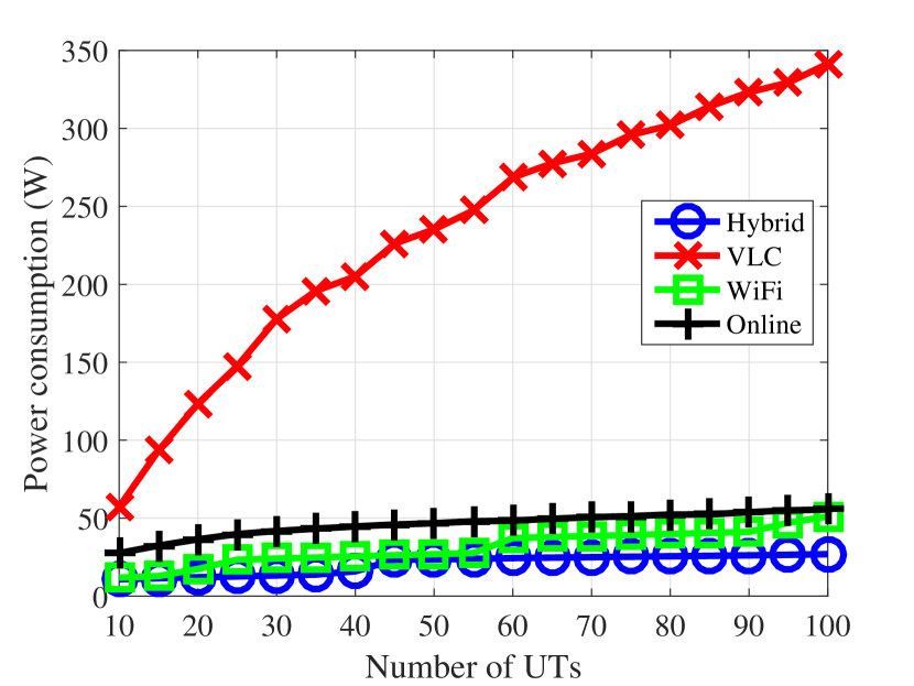
(b) $\eta_{m}^{AC}=0.07$

(c) $\eta_{m}^{AC}=0.08$

(d) $\eta_{m}^{AC}=0.09$

Figure 7: Power consumption in terms of number of UTs at day

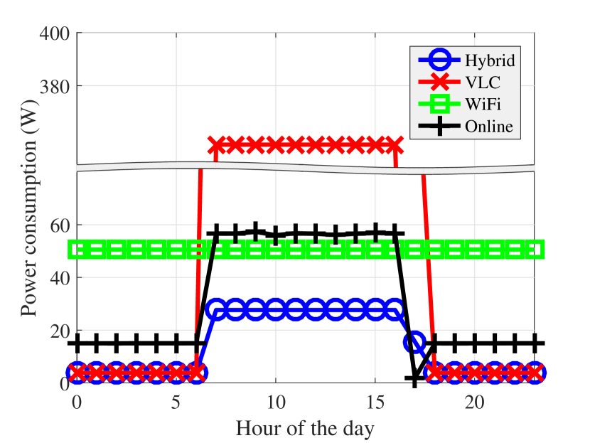
(a) $\eta_{m}^{AC}=0.06$

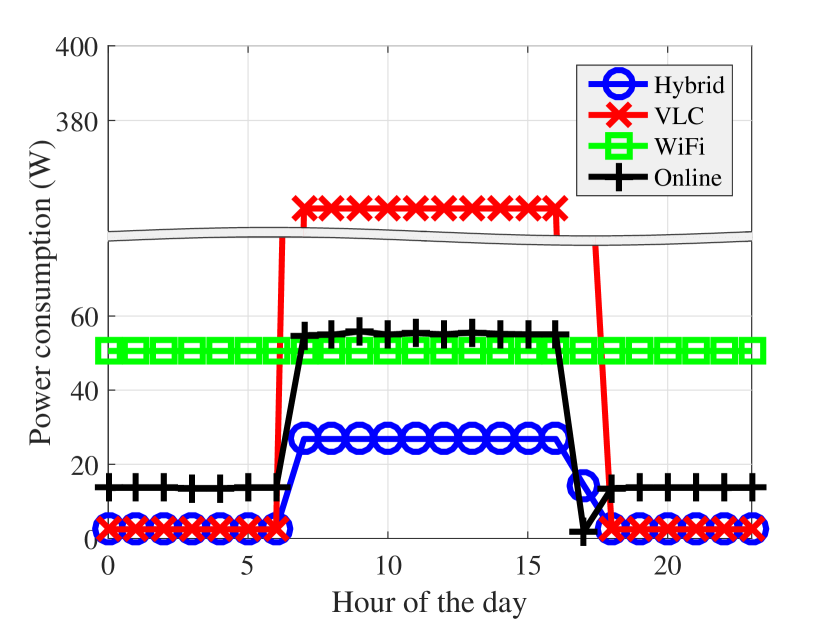
(b) $\eta_{m}^{AC}=0.07$

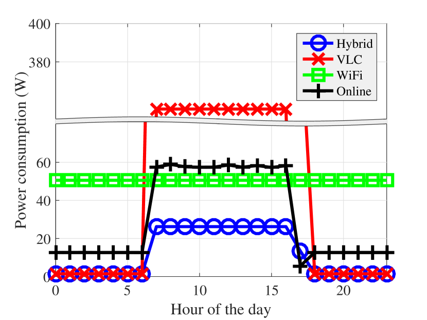
(c) $\eta_{m}^{AC}=0.08$

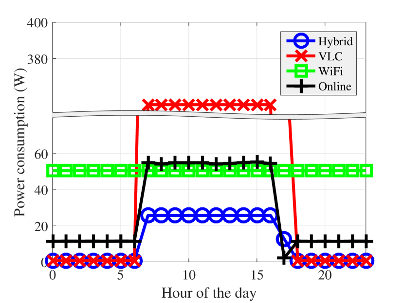
(d) $\eta_{m}^{AC}=0.09$

Figure 8: Power consumption in terms of hour of the day

In Fig. 13 to 13, we present simulation results of two modified versions of our proposed online algorithm. The first version, named “Online WiFi”, is our online algorithm when only the WiFi APs are considered. The second version, named “Online VLC”, is our online algorithm when only the VLC APs are considered. In Fig. 13 and Fig. 13, 100 UTs are distributed uniformly at random. At night (Fig. 13), the power consumption of our proposed algorithm and the Online VLC scheme are lower than that of the Online WiFi scheme, as all the VLC APs are turned on for illumination. The sudden increase in power consumption for the Online WiFi scheme is due to turning on additional WiFi APs. During the day (Fig. 13), the VLC APs may be forced to be turned on when the number of UTs is large, resulting in unnecessary illumination and higher power consumption for the Online VLC scheme compared to our proposed algorithm and the Online WiFi scheme. We also note that the performance of the proposed algorithm is better than that of the Online WiFi scheme, since some of the UTs are located in the square region (i.e., where there are no windows) and the VLC APs are already turned on for illumination. Our proposed algorithm takes advantage of those turned on VLC APs to provide communication at a lower power consumption.

In Fig. 13 and Fig. 13, the throughput requirement per UT is set to 6 Mbps. During the night (Fig. 13), where all the VLC APs are turned on for illumination, our proposed algorithm and the Online VLC scheme perform better than the Online WiFi scheme. We also note that the power consumption of the Online VLC scheme is similar to the power consumption of the optimal VLC scheme shown in Fig. 9. This shows that our proposed algorithm can be used to determine the assignment of UTs to APs at a much lower complexity while achieveing similar power consumptions.

In Fig. 13, the number of UTs is set to 100 and the throughput requirement per UT is set to 6 Mbps. From the figure, we note that, from 6am to 7pm, the Online WiFi scheme consumes less power than the Online VLC scheme due to the large power consumption of turning on VLC APs. We also see that our proposed hybrid algorithm performs better than both the Online WiFi and the Online VLC schemes during the day. This is due to the fact that our proposed algorithm can take advantage of the already turned on VLC APs for illumination in the square region and the WiFi APs for the external rooms. From 7pm to 6am, since all VLC APs are turned on for illumination, the power consumption of the Online VLC scheme and our proposed algorithm is less than the power consumption of the Online WiFi.

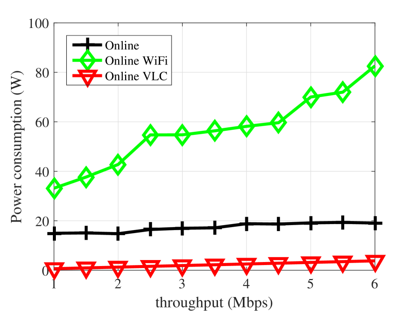
(a) $\eta_{m}^{AC}=0.06$

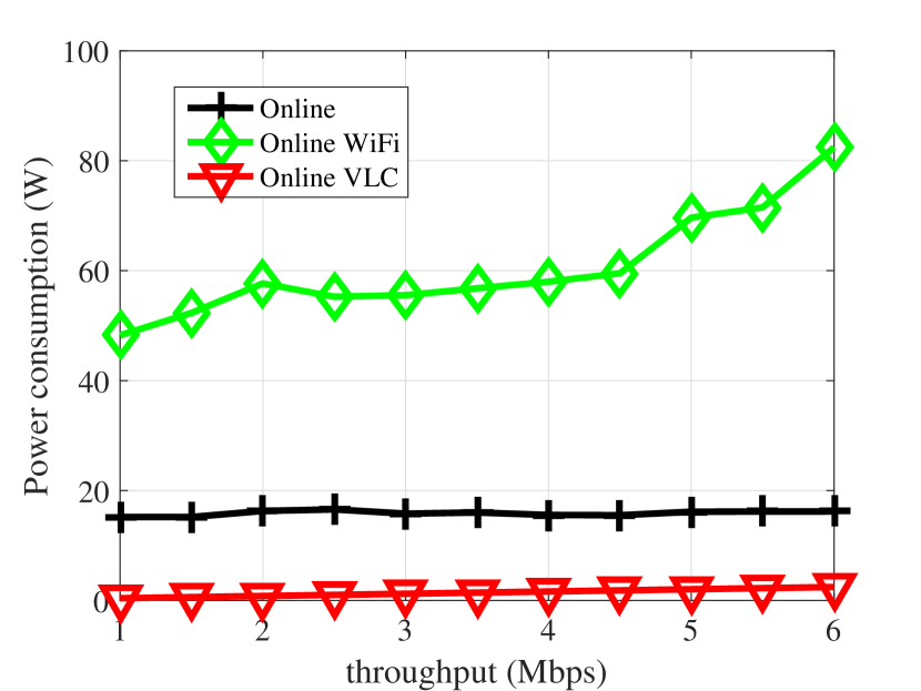
(b) $\eta_{m}^{AC}=0.07$

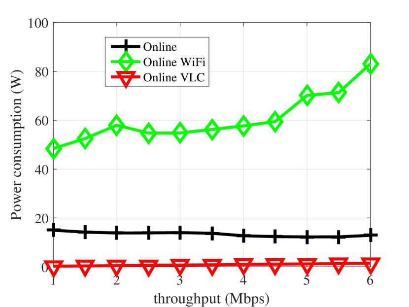
(c) $\eta_{m}^{AC}=0.08$

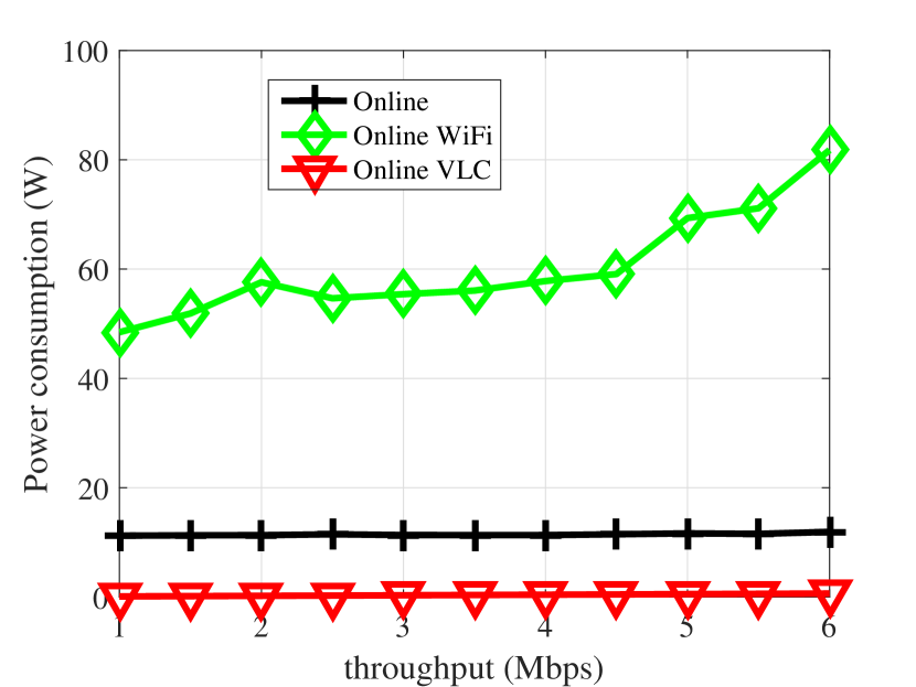
(d) $\eta_{m}^{AC}=0.09$

Figure 9: Power consumption in terms of throughput requirement per user at night

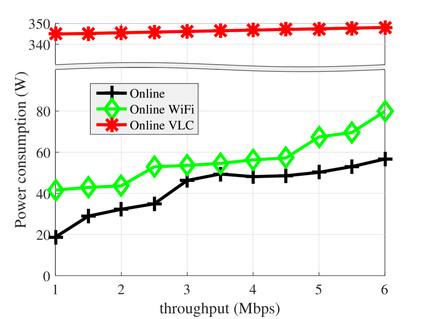
(e) $\eta_{m}^{AC}=0.06$

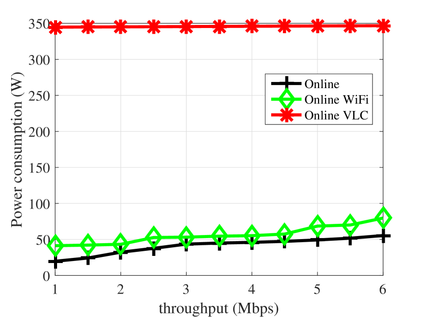
(f) $\eta_{m}^{AC}=0.07$

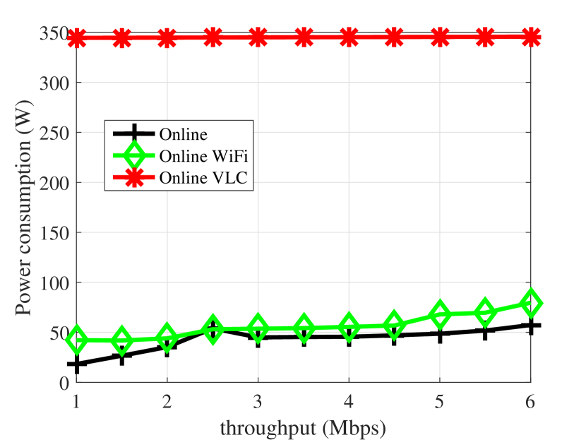
(g) $\eta_{m}^{AC}=0.08$

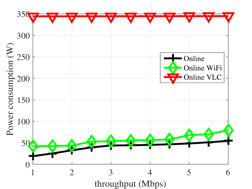
(h) $\eta_{m}^{AC}=0.09$

Figure 10: Power consumption in terms of throughput requirement per user at day

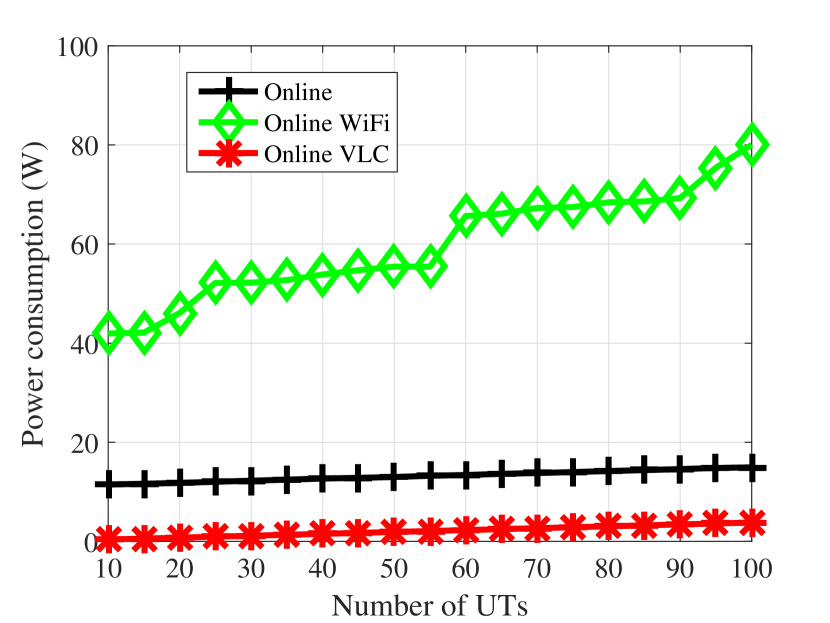
(a) $\eta_{m}^{AC}=0.06$

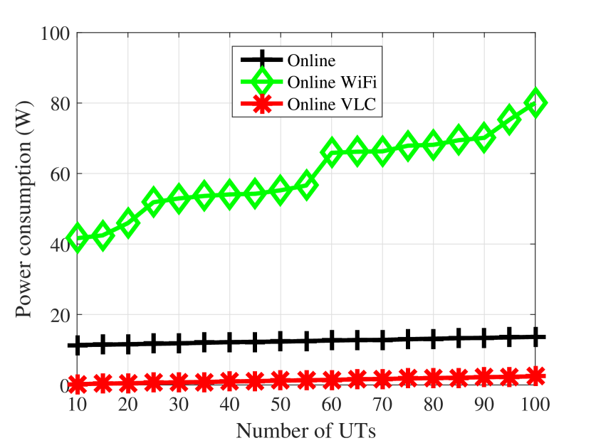
(b) $\eta_{m}^{AC}=0.07$

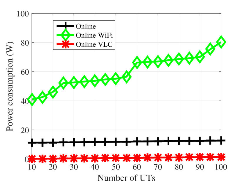
(c) $\eta_{m}^{AC}=0.08$

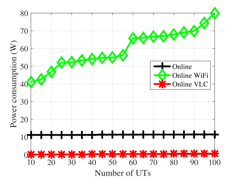
(d) $\eta_{m}^{AC}=0.09$

Figure 11: Power consumption in terms of number of UTs at night

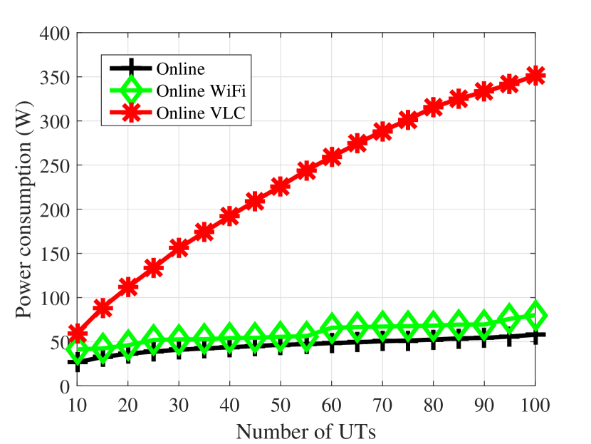
(a) $\eta_{m}^{AC}=0.06$

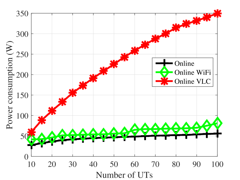
(b) $\eta_{m}^{AC}=0.07$

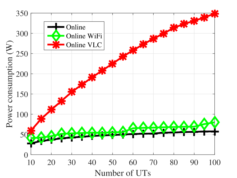
(c) $\eta_{m}^{AC}=0.08$

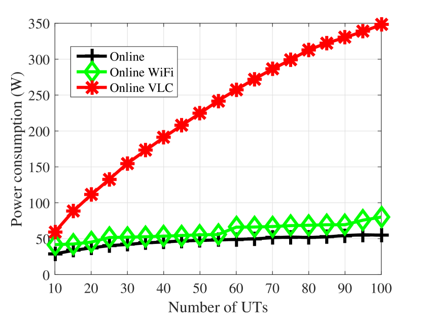
(d) $\eta_{m}^{AC}=0.09$

Figure 12: Power consumption in terms of number of UTs at day

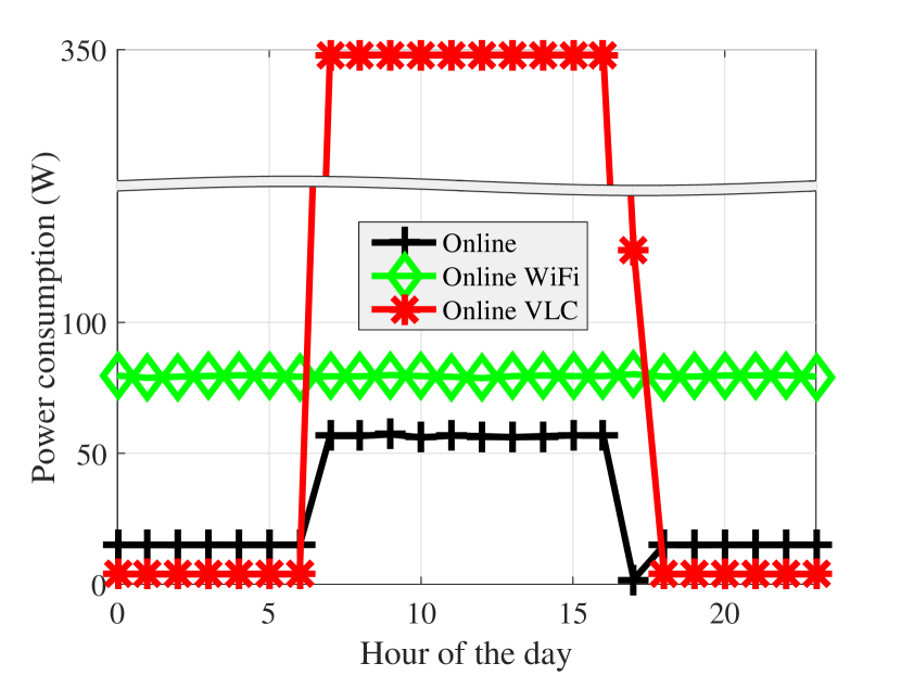
(a) $\eta_{m}^{AC}=0.06$

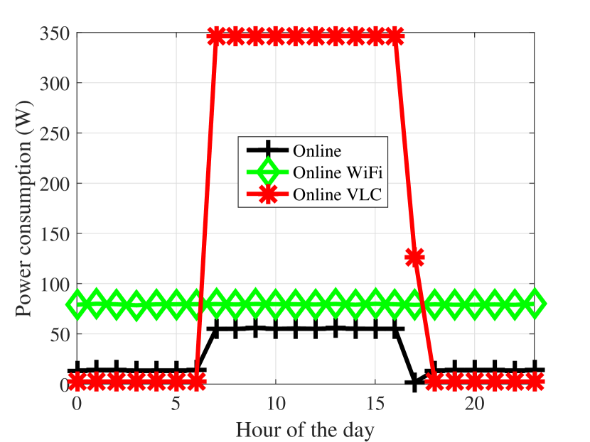
(b) $\eta_{m}^{AC}=0.07$

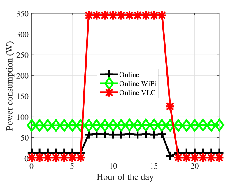
(c) $\eta_{m}^{AC}=0.08$

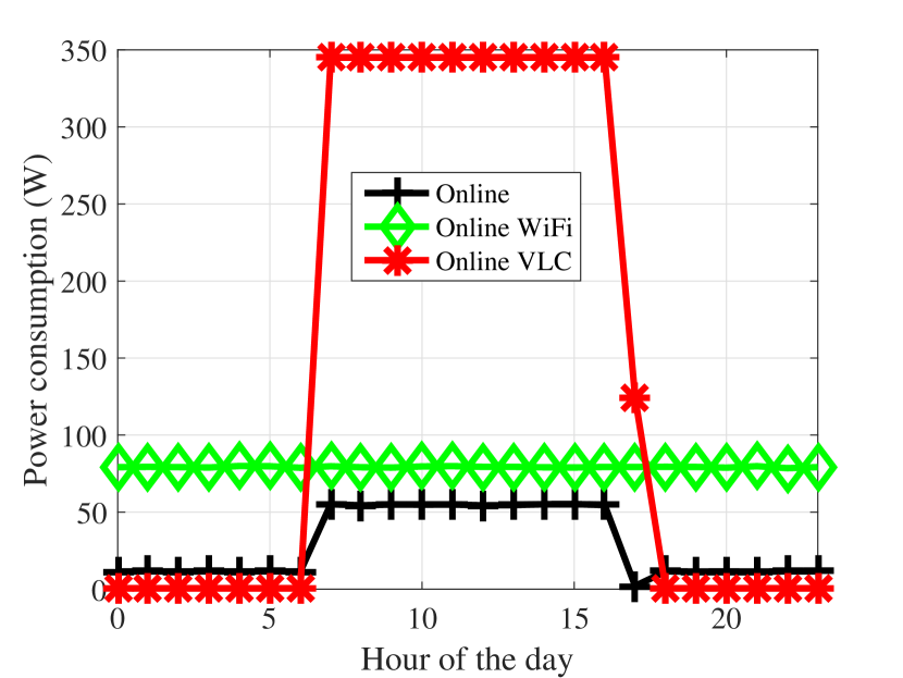
(d) $\eta_{m}^{AC}=0.09$

Figure 13: Power consumption in terms of hour of the day

VII Conclusion

In this paper, we have tackled the problem of reducing the power consumption of wireless indoor access networks. Unlike previous works, we utilize VLC, which can jointly provide communications and illumination, and thus greatly reduces the power consumption. However, in a sunny day or with a large number of users, the RF access methods will be more energy efficient than VLC. Our proposed system is a hybrid one comprising both VLC and WiFi access methods. We formulate the problem of minimizing the power consumption of the system while satisfying the requests of the users and achieving the desired illumination level. The problem is NP-complete. To alleviate the complexity, we design an online algorithm for the problem with good competitive ratio. Our simulation results show that the proposed hybrid system has the potential to reduce the power consumption by more than 75% over the individual WiFi and VLC systems.

References

- [1] “Informa telecoms & media, “mobile access at home,” 2008.”
- [2] “GBI research“visible light communication (VLC) - a potential solution to the global wireless spectrum shortage”, 2011.”
- [3] “Ericsson report optimizing the indoor experience,” http://www.ericsson.com/res/docs/2013/real-performance-indoors.pdf, [Online].
- [4] “In-Building Wireless: One Size does not fit all,” https://www.alcatel-lucent.com/solutions/in-building/in-building-infographic, [Online].
- [5] “Cisco Service Provider Wi-Fi: A Platform for Business Innovation and Revenue Generation,” http://www.cisco.com/c/en/us/solutions/collateral/service-provider/service-provider-wi-fi/solution_overview_c22-642482.html, [Online].
- [6] “Cisco Visual Networking Index,” http://www.cisco.com/c/en/us/solutions/collateral/service-provider/visual-networking-index-vni/white_paper_c11-520862.html, [Online].
- [7] S. Hargreaves, “The Internet: One big power suck,” http://money.cnn.com/2011/05/03/technology/internet_electricity/, 2011, [Online].
- [8] “Cisco visual networking index,” http://www.cisco.com/c/en/us/solutions/service-provider/visual-networking-index-vni/white-paper-listing.html, 2014, [Online].
- [9] “The Global Public Wi-Fi Network Grows to 50 Million Worldwide Wi-Fi Hotspots,” http://www.ipass.com/press-releases/the-global-public-wi-fi-network-grows-to-50-million-worldwide-wi-fi-hotspots/, [Online].
- [10] “Electricity usage of a Wi-Fi Router,” http://energyusecalculator.com/electricity_wifirouter.htm, [Online].
- [11] E. Shih, P. Bahl, and M. Sinclair, “Wake on wireless: an event driven energy saving strategy for battery operated devices,” in Proceedings of the 8th annual international conference on Mobile computing and networking. ACM, 2002, pp. 160–171.
- [12] E. Rozner, V. Navda, R. Ramjee, and S. Rayanchu, “Napman: network-assisted power management for wifi devices,” in Proceedings of the 8th international conference on Mobile systems, applications, and services. ACM, 2010, pp. 91–106.
- [13] J. Liu and L. Zhong, “Micro power management of active 802.11 interfaces,” in Proceedings of the 6th international conference on Mobile systems, applications, and services. ACM, 2008, pp. 146–159.
- [14] J. Manweiler and R. Choudhury, “Avoiding the rush hours: Wifi energy management via traffic isolation,” in Proceedings of the 9th international conference on Mobile systems, applications, and services. ACM, 2011, pp. 253–266.
- [15] W. Ye, J. Heidemann, and D. Estrin, “An energy-efficient mac protocol for wireless sensor networks,” in INFOCOM, vol. 3. IEEE, 2002, pp. 1567–1576.
- [16] S. Sen, R. Choudhury, and S. Nelakuditi, “Csma/cn: carrier sense multiple access with collision notification,” IEEE/ACM Transactions on Networking (TON), vol. 20, no. 2, pp. 544–556, 2012.
- [17] S. Sen, R. Choudhury, and B. Radunovic, “Phy-assisted energy management for mobile devices,” Proc. ACM MobiSys Poster Session, 2010.
- [18] T. Han and N. Ansari, “On greening cellular networks via multicell cooperation,” Wireless Communications, IEEE, vol. 20, no. 1, pp. 82–89, 2013.
- [19] ——, “On optimizing green energy utilization for cellular networks with hybrid energy supplies,” Wireless Communications, vol. 12, no. 8, pp. 3872–3882, 2013.
- [20] ——, “A traffic load balancing framework for software-defined radio access networks powered by hybrid energy sources,” IEEE Transactions on Networking, DOI: 10.1109/TNET.2015.2404576, early access,, 2015.
- [21] “What are the major uses of electricity?” http://shrinkthatfootprint.com/how-do-we-use-electricity, [Online].
- [22] S. Tsuzuki, I. Areni, and Y. Yamada, “A feasibility study of 1Gbps PLC system assuming a high-balanced DC power-line channel,” in Power Line Communications and Its Applications (ISPLC). IEEE, 2012, pp. 386–391.
- [23] A. Tonello, P. Siohan, A. Zeddam, and X. Mongaboure, “Challenges for 1 Gbps power line communications in home networks,” in Personal, Indoor and Mobile Radio Communications. IEEE, 2008, pp. 1–6.
- [24] M. Kavehrad, “Optical wireless applications: A solution to ease the wireless airwaves spectrum crunch,” in SPIE OPTO. International Society for Optics and Photonics, 2013, pp. 86 450G–86 450G.
- [25] M. Giordani, M. Mezzavilla, S. Rangan, and M. Zorzi, “Multi-connectivity in 5G mmWave cellular networks,” in Ad Hoc Networking Workshop (Med-Hoc-Net), 2016 Mediterranean. IEEE, 2016, pp. 1–7.
- [26] A. Asadi and V. Mancuso, “WiFi Direct and LTE D2D in action,” in Wireless Days (WD), 2013 IFIP. IEEE, 2013, pp. 1–8.
- [27] E. Arribas and V. Mancuso, “Multi-path D2D leads to satisfaction,” in A World of Wireless, Mobile and Multimedia Networks (WoWMoM), 2017 IEEE 18th International Symposium on. IEEE, 2017, pp. 1–7.
- [28] L. Feng, R. Q. Hu, J. Wang, P. Xu, and Y. Qian, “Applying VLC in 5G networks: Architectures and key technologies,” IEEE Network, vol. 30, no. 6, pp. 77–83, 2016.
- [29] D. A. Basnayaka and H. Haas, “Hybrid RF and VLC systems: Improving user data rate performance of VLC systems,” in Vehicular Technology Conference (VTC Spring), 2015 IEEE 81st. IEEE, 2015, pp. 1–5.
- [30] S. Shao, A. Khreishah, M. B. Rahaim, H. Elgala, M. Ayyash, T. D. Little, and J. Wu, “An indoor hybrid wifi-vlc internet access system,” in IEEE MASS, 2014, pp. 569–574.
- [31] S. Shao, A. Khreishah, M. Ayyash, M. B. Rahaim, H. Elgala, V. Jungnickel, D. Schulz, T. D. Little, J. Hilt, and R. Freund, “Design and analysis of a visible-light-communication enhanced WiFi system,” IEEE/OSA Journal of Optical Communications and Networking (JOCN), vol. 7, no. 10, 2015.
- [32] H. Chowdhury, I. Ashraf, and M. Katz, “Energy-efficient connectivity in hybrid radio-optical wireless systems,” in ISWCS, 2013, pp. 1–5.
- [33] M. Kashef, M. Ismail, M. Abdallah, K. A. Qaraqe, and E. Serpedin, “Energy efficient resource allocation for mixed rf/vlc heterogeneous wireless networks,” IEEE Journal on Selected Areas in Communications, vol. 34, no. 4, pp. 883–893, 2016.
- [34] M. Kafafy, Y. Fahmy, M. Abdallah, and M. Khairy, “Power Efficient Downlink Resource Allocation for Hybrid RF/VLC Wireless Networks,” in IEEE Wireless Communications and Networking Conference (WCNC), 2017, pp. 1–6.
- [35] M. Kashef, M. Abdallah, and N. Al-Dhahir, “Transmit Power Optimization for a Hybrid PLC/VLC/RF Communication System,” IEEE Transactions on Green Communications and Networking, 2017.
- [36] A. Siddique and M. Tahir, “Joint brightness control and data transmission for visible light communication systems based on white leds,” in Consumer Communications and Networking Conference (CCNC), 2011 IEEE. IEEE, 2011, pp. 1026–1030.
- [37] H. Sugiyama, S. Haruyama, and M. Nakagawa, “Brightness control methods for illumination and visible-light communication systems,” in Wireless and Mobile Communications, 2007. ICWMC’07. Third International Conference on. IEEE, 2007, pp. 78–78.
- [38] K. Lee and H. Park, “Modulations for visible light communications with dimming control,” Photonics Technology Letters, IEEE, vol. 23, no. 16, pp. 1136–1138, 2011.
- [39] I. Din and H. Kim, “Energy-efficient brightness control and data transmission for visible light communication,” IEEE Photonics Technology Letters, vol. 26, pp. 781–784, 2014.
- [40] S. Shao, A. Khreishah, M. Ayyash, M. Rahaim, H. Elgala, V. Jungnickel, D. Schulz, and T. Little, “Design of a visible-light-communication enhanced WiFi system,” arXiv preprint arXiv:1503.02367, 2015.
- [41] X. Deng, Y. Wu, K. Arulandu, G. Zhou, and J. Linnartz, “Performance comparison for illumination and visible light communication system using buck converters,” in IEEE Globecom Workshops, 2014.
- [42] Z. Ghassemlooy, W. Popoola, and S. Rajbhandari, Optical wireless communications: system and channel modelling with Matlab®. CRC Press, 2012.
- [43] L. Grobe, A. Paraskevopoulos, J. Hilt, D. Schulz, F. Lassak, F. Hartlieb, C. Kottke, V. Jungnickel, and K. Langer, “High-speed visible light communication systems,” IEEE Communications Magazine, vol. 51, no. 12, pp. 60–66, 2013.
- [44] K. Langer, J. Hilt, D. Shulz, F. Lassak, F. Hartlieb, C. Kottke, L. Grobe, V. Jungnickel, and A. Paraskevopoulos, “Optoelectronics & communications rate-adaptive visible light communication at 500Mb/s arrives at plug and play,” SPIE Newsroom, vol. 14, 2013.
- [45] T. Komine and M. Nakagawa, “Fundamental analysis for visible-light communication system using LED lights,” IEEE Transactions on Consumer Electronics, vol. 50, no. 1, pp. 100–107, 2004.
- [46] M. Khan, V. Dave, Y. Chen, O. Jensen, L. Qiu, A. Bhartia, and S. Rallapalli, “Model-driven energy-aware rate adaptation,” in Proceedings of the fourteenth ACM international symposium on Mobile ad hoc networking and computing. ACM, 2013, pp. 217–226.
- [47] J. Huang, F. Qian, A. Gerber, Z. Mao, S. Sen, and O. Spatscheck, “A close examination of performance and power characteristics of 4G LTE networks,” in Proceedings of the 10th international conference on Mobile systems, applications, and services. ACM, 2012, pp. 225–238.
- [48] R. Friedman, A. Kogan, and Y. Krivolapov, “On power and throughput tradeoffs of wifi and bluetooth in smartphones,” Mobile Computing, IEEE Transactions on, vol. 12, no. 7, pp. 1363–1376, 2013.
- [49] L. Sun, R. Sheshadri, W. Zheng, and D. Koutsonikolas, “Modeling wifi active power/energy consumption in smartphones,” in Distributed Computing Systems (ICDCS), 2014 IEEE 34th International Conference on. IEEE, 2014, pp. 41–51.
- [50] J. Zhang, X. Zhang, and G. Wu, “Dancing with light: Predictive in-frame rate selection for visible light networks,” in INFOCOM, 2015 Proceedings IEEE. IEEE, 2015, pp. 1–9.
- [51] K. Mabell and G. Chavez, “Energy efficiency in wireless access networks: Measurements, models and algorithms,” Ph.D. dissertation, University of Trento, 2013.
- [52] X. Zhang and K. Shin, “E-mili: energy-minimizing idle listening in wireless networks,” Mobile Computing, IEEE Transactions on, vol. 11, no. 9, pp. 1441–1454, 2012.
- [53] L. Barroso and U. Hölzle, “The case for energy-proportional computing,” IEEE computer, vol. 40, no. 12, pp. 33–37, 2007.
- [54] V. Valancius, N. Laoutaris, L. M. andC. Diot, and P. Rodriguez, “Greening the internet with nano data centers,” in Proceedings of the 5th international conference on Emerging networking experiments and technologies. ACM, 2009, pp. 37–48.
- [55] C. Gunaratne, K. Christensen, and B. Nordman, “Managing energy consumption costs in desktop PCs and LAN switches with proxying, split TCP connections, and scaling of link speed,” International Journal of Network Management, vol. 15, no. 5, pp. 297–310, 2005.
- [56] Z. Tian, K. Wright, and X. Zhou, “The darklight rises: Visible light communication in the dark,” in ACM MobiCom, 2016, pp. 495–496.
- [57] I. ILOG, “Cplex optimizer, version 12.6.1,” http://www-03.ibm.com/software/products/de/ibmilogcpleoptistud/, 2014, [Online].
- [58] N. Buchbinder and J. Naor, “The design of competitive online algorithms via a primal: dual approach,” Foundations and Trends® in Theoretical Computer Science, vol. 3, no. 2–3, pp. 93–263, 2009.
- [59] Wikipedia, “Maximum flow problem.” [Online]. Available: https://en.wikipedia.org/wiki/Maximum_flow_problem Accessed on January 2018.
- [60] ——, “Maximum flow problem.” [Online]. Available: https://en.wikipedia.org/wiki/Maximum\_flow\_problem (Accessed on January 2018).
- [61] “Cplex, http://www-01.ibm.com/software/commerce/optimization/cplex-optimizer/.”
- [62] S. Shao, A. Khreishah, and I. Khalil, “Joint link scheduling and brightness control for greening VLC-based indoor access networks,” arXiv preprint arXiv:1510.00026, 2015.
- [63] T. BRIGHT, “Efficient blue light-emitting diodes leading to bright and energy-saving white light sources,” https://www.nobelprize.org/nobel_prizes/physics/laureates/2014/advanced-physicsprize2014.pdf, 2014, [Online].
- [64] T. M. Cover and J. A. Thomas, Elements of information theory. John Wiley & Sons, 2012.
- [65] L. Zyga, “White LEDs with super-high luminous efficacy could satisfy all general lighting needs,” http://phys.org/news/2010-08-white-super-high-luminous-efficacy.html, 2010, [Online].
- [66] “Legit reviews.” [Online]. Available: http://www.legitreviews.com/asus-rt-ac66u-802-11ac-wireless-ac1750-router-review_2207/5
- [67] D. House, “Rf propagation: A study of wifi design for the department of veterans affairs,” https://www.catapulttechnology.com/pdf/Insights_Files/white_papers/RF_Propagation_White_Paper.pdf, 2010, [Online].
- [68] T. Kessler, “Diagnosing and addressing wi-fi signal quality problems,” http://www.cnet.com/news/diagnosing-and-addressing-wi-fi-signal-quality-problems/, 2011, [Online].
- [69] T. S. Rappaport et al., Wireless communications: principles and practice, 1996, vol. 2.
- [70] J.-P. Ebert, S. Aier, G. Kofahl, A. Becker, B. Burns, and A. Wolisz, “Measurement and simulation of the energy consumption of an wlan interface,” Technical University of Berlin, Telecommunication Networks Group, Tech. Rep. TKN-02-010, 2002.
- [71] D. H. Li and G. Cheung, “Average daylight factor for the 15 cie standard skies,” Lighting Research and Technology, vol. 38, no. 2, pp. 137–149, 2006.
- [72] P. J. Littlefair, “Measurements of the luminous efficacy of daylight,” Lighting Research and technology, vol. 20, no. 4, pp. 177–188, 1988.
- [73] S. R. Data, “Solar radiation data.” [Online]. Available: http://www.soda-pro.com/home