Stochastic stability of the classical Lorenz flow under impulsive type forcing

Abstract

We introduce a novel type of random perturbation for the classical Lorenz flow in order to better model phenomena slowly varying in time such as anthropogenic forcing in climatology and prove stochastic stability for the unperturbed flow. The perturbation acts on the system in an impulsive way, hence is not of diffusive type as those already discussed in [Ki], [Ke], [Me]. Namely, given a cross-section $\mathcal{M}$ for the unperturbed flow, each time the trajectory of the system crosses $\mathcal{M}$ the phase velocity field is changed with a new one sampled at random from a suitable neighborhood of the unperturbed one. The resulting random evolution is therefore described by a piecewise deterministic Markov process. The proof of the stochastic stability for the umperturbed flow is then carryed on working either in the framework of the Random Dynamical Systems or in that of semi-Markov processes.

AMS subject classification:

34F05, 93E15.

Keywords and phrases:

Random perturbations of dynamical systems, classical Lorenz model, random dynamical systems, semi-Markov random evolutions, piecewise deterministic Markov processes, Lorenz’63 model, anthropogenic forcing.

Acknowledgement:

M. Gianfelice was partially supported by LIA LYSM AMU-CNRS-ECM-INdAM. S. Vaienti was supported by the Leverhulme Trust for support thorough the Network Grant IN-2014-021 and by the project APEX Systèmes dynamiques: Probabilités et Approximation Diophantienne PAD funded by the Région PACA (France). S.Vaienti warmly thanks the Laboratoire International Associé LIA LYSM, the LabEx Archimède (AMU University, Marseille), the INdAM (Italy) and the UMI-CNRS 3483 Laboratoire Fibonacci (Pisa) where this work has been completed under a CNRS delegation.

Part I Introduction, notations and results

1 The classical Lorenz flow

The physical behaviour of turbulent systems such the atmosphere are usually modeled by flows exhibiting a sensitive dependence on the initial conditions. The behaviour of the trajectories of the system in the phase space for large times is usually numerically very hard to compute and consequently the same computational difficulty affects also the computation of the phase averages of physically relevant observables. A way to overcome this problem is to select a few of these relevant observables under the hypothesis that the statistical properties of the smaller system defined by the evolution of such quantities can capture the important features of the statistical behaviour of the original system [NVKDF].

As a matter of fact this turns out to be the case when considering classical Lorenz model, a.k.a. Lorenz’63 model in the physics literature, i.e. the system of equation

$$\left\{\begin{array}[c]{l}\dot{x}_{1}=-\zeta x_{1}+\zeta x_{2}\\ \dot{x}_{2}=-x_{1}x_{3}+\gamma x_{1}-x_{2}\\ \dot{x}_{3}=x_{1}x_{2}-\beta x_{3}\end{array}\right.\ ,$$ (1)

which was introduced by Lorenz in his celebrated paper [Lo] as a simplified yet non trivial model for thermal convection of the atmosphere and since then it has been pointed out as the typical real example of a non-hyperbolic three-dimensional flow whose trajectories show a sensitive dependence on initial conditions. In fact, the classical Lorenz flow, for $\zeta=10,\gamma=28,\beta=8/3,$ has been proved in [Tu], and more recently in [AM], to show the same dynamical features of its ideal counterpart the so called geometric Lorenz flow, introduced in [ABS] and in [GW], which represents the prototype of a three-dimensional flow exhibiting a partially hyperbolic attractor [AP]. The Lorenz’63 model, indeed, has the interesting feature that it can be rewritten as

$$\left\{\begin{array}[c]{l}\dot{y}_{1}=-\zeta y_{1}+\zeta y_{2}\\ \dot{y}_{2}=-y_{1}y_{3}-\gamma y_{1}-y_{2}\\ \dot{y}_{3}=y_{1}y_{2}-\beta y_{3}-\beta\left(\gamma+\zeta\right)\end{array}\right.\ ,$$ (2)

showing the corresponding flow to be generated by the sum of a Hamiltonian $SO\left(3\right)$-invariant field and a gradient field (we refer the reader to [GMPV] and references therein). Therefore, as it has been proved in [GMPV], the invariant measure of the classical Lorenz flow can be constructed starting from the invariant measure of the one-dimensional system describing the evolution of the extrema of the first integrals of the associated Hamiltonian flow.

1.1 Stability of the invariant measure of the Lorenz’63 flow

Since $C^{1}$ perturbations of the classical Lorenz vector field admit a $C^{1+\epsilon}$ stable foliation [AM] and since the geometric Lorenz attractor is robust in the $C^{1}$ topology [AP], it is natural to discuss the statistical and the stochastic stability of the classical Lorenz flow under this kind of perturbations.

Indeed, in applications to climate dynamics, when considering the Lorenz’63 flow as a model for the atmospheric circulation, the analysis of the stability of the statistical properties of the unperturbed flow under perturbations of the velocity phase field of this kind can turn out to be a useful tool in the study of the so called anthropogenic climate change [CMP].

1.1.1 Statistical stability

For what concerns the statistical stability, in [GMPV] it has been shown that the effect of an additive constant perturbation term to the classical Lorenz vector field results into a particular kind of perturbation of the map of the interval describing the evolution of the maxima of the Casimir function for the (+) Lie-Poisson brackets associated to the $so\left(3\right)$ algebra. Moreover, it has been proved that the invariant measures for the perturbed and for the unperturbed 1-$d$ maps of this kind have Lipschitz continuous density and that the unperturbed invariant measure is strongly statistically stable. Since the SRB measure of the classical Lorenz flow can be constructed starting from the invariant measure of the one-dimensional map obtained through reduction to the quotient leaf space of the Poincaré map on a two-dimensional manifold transverse to the flow [AP], the statistical stability for the invariant measure of this map implies that of the SRB measure of the unperturbed flow. Other results in this direction are given in [AS], [BR] and [GL] where strong statistical stability of the geometric Lorenz flow is analysed.

1.1.2 Random perturbations

Random perturbations of the classical Lorenz flow have been studied in the framework of stochastic differential equations [Sc], [CSG], [Ke] (see also [Ar] and reference therein). The main interest of these studies was bifurcation theory and the existence and the characterization of the random attractor. The existence of the stationary measure for this stochastic version of the system of equations given in (2) is proved in [Ke].

Stochastic stability under diffusive type perturbations has been studied in [Ki] for the geometric Lorenz flow and in [Me] for the contracting Lorenz flow.

2 Physical motivation

The analysis of the stability of the statistical properties of the classical Lorenz flow can provide a theoretical framework for the study of climate changes, in particular those induced by the anthropogenic influence on climate dynamics.

A possible way to study this problem is to add a weak perturbing term to the phase vector field generating the atmospheric flow which model the atmospheric circulation: the so called anthropogenic forcing. Assuming that the atmospheric circulation is described by a model exhibiting a robust singular hyperbolic attractor, as it is the case for the classical Lorenz flow, it has been shown empirically that the effect of the perturbation can possibly affect just the statistical properties of the system [Pa], [CMP]. Therefore, because of its very weak nature (small intensity and slow variability in time), a practical way to measure the impact of the anthropogenic forcing on climate statistics is to look at the extreme value statistics of those particular observables whose evolution may be more sensitive to it [Su]. In the particular case these observables are given by bounded (real valued) functions on the phase space, an effective way to look at their extreme value statistics is to look first at the statistics of their extrema and then eventually to the extreme value statistics of these.

We stress that the result presented in [GMPV] fit indeed in this framework since, starting from the assumption made in [Pa] and [CMP] that, taking the classical Lorenz flow as a model for the atmospheric circulation, the effect of the anthropogenic influence on climate dynamics can be modeled by the addition of a small constant term to the unperturbed phase vector field, it has been shown that the statistics of the extrema of the first integrals of the Hamiltonian flow underlying the classical Lorenz one, which are global observables for this system, are very sensitive to this kind of perturbation (see e.g. Example 8 in [GMPV]).

Of course, a more realistic model for the anthropogenic forcing should take into account random perturbations of the phase vector field rather than deterministic ones. Anyway it seems unlikely that the resulting process can be a diffusion, since in this case the driving process fluctuates faster than what it is assumed to do in principle a perturbing term of the type just described.

2.1 Modeling random perturbations of impulsive type

We introduce a random perturbation of the Lorenz’63 flow which, being of impulsive nature, differ from diffusion-type perturbations.

For any realization of the noise $\eta\in\left[-\varepsilon,\varepsilon\right],$ we consider a flow $\left(\Phi_{\eta}^{t},t\geq 0\right)$ generated by the phase vector field $\phi_{\eta}$ belonging to a sufficiently small neighborhood of the classical Lorenz one in the $C^{1}$ topology. For $\varepsilon$ small enough, the realizations of the perturbed phase vector field $\phi_{\eta}$ can be chosen such that there exists an open neighborhood $U$ of the unperturbed attractor in $\mathbb{R}^{3},$ independent of the noise parameter $\eta,$ containing the attractor of any realization of $\phi_{\eta}$ and, moreover, such that a given Poincaré section $\mathcal{M}$ for the unperturbed flow is also transversal to any realization of the perturbed one. Thus, given $\mathcal{M},$ the random process describing the perturbation is constructed selecting at random, in an independent way, the value of $\phi_{\eta}$ at the crossing of $\mathcal{M}$ by the phase trajectory.

This procedure defines a semi-Markov random evolution [KS], in fact a piecewise deterministic Markov process (PDMP) [Da].

Therefore, the major object of this paper will be to show the existence of a stationary measure for the imbedded Markov chain driving the random process just described as well as to prove that the stationary process weakly converges, as $\varepsilon$ tends to $0,$ to the physical measure of the unperturbed one.

More specifically, let $\hat{\tau}_{\eta}:U\rightarrow\mathcal{M}$ and $\tau_{\eta}:\mathcal{M}\circlearrowleft$ be respectively the hitting time of $\mathcal{M}$ and the return time map on $\mathcal{M}$ for $\left(\Phi_{\eta}^{t},t\geq 0\right).$ If $\eta$ is sampled according to a given law $\lambda_{\varepsilon}$ supported on $\left[-\varepsilon,\varepsilon\right],$ the sequence $\left\{\mathfrak{x}_{i}\right\}_{i\geq 0}$ such that $\mathfrak{x}_{0}\in\mathcal{M}$ and, for $i\geq 0,\mathfrak{x}_{i+1}:=\Phi_{\eta}^{\tau_{\eta}\left(\mathfrak{x}_{i}\right)}\left(\mathfrak{x}_{i}\right)$ is a homogeneous Markov chain on $\mathcal{M}$ with transition probability measure

$$\mathbb{P}\left\{\mathfrak{x}_{1}\in dz|\mathfrak{x}_{0}\right\}=\lambda_{\varepsilon}\left\{\eta\in\left[-1,1\right]:R_{\eta}\left(\mathfrak{x}_{0}\right)\in dz\right\}\ .$$ (3)

Considering the collection of sequences of i.i.d.r.v’s $\left\{\eta_{i}\right\}_{i\geq 0}$ distributed according to $\lambda_{\varepsilon},$ we define the random sequence $\left\{\sigma_{n}\right\}_{n\geq 1}\in\mathbb{R}$ such that $\sigma_{n}:=\sum_{i=0}^{n-1}\tau_{\eta_{i-1}}\left(\mathfrak{x}_{i-1}\right),n\geq 1.$ Then, it is easily checked that the sequence $\left\{\left(\mathfrak{x}_{n},\mathbf{t}_{n}\right)\right\}_{n\geq 0}$ such that $\mathbf{t}_{0}:=\sigma_{1}$ and, for $n\geq 0,\mathbf{t}_{n}:=\sigma_{n+1}-\sigma_{n}$ is a Markov renewal process (MRP) [As], [KS]. Therefore, denoting by $\left(\mathbf{N}_{t},t\geq 0\right),$ such that $\mathbf{N}_{0}:=0$ and $\mathbf{N}_{t}:=\sum_{n\geq 0}\mathbf{1}_{\left[0,t\right]}\left(\sigma_{n}\right),$ the associated counting process and defining:

• $\left(\mathfrak{x}_{t},t\geq 0\right),$ such that $\mathfrak{x}_{t}:=\mathfrak{x}_{\mathbf{N}_{t}},$ the associated semi-Markov process;

• $\left(\mathfrak{l}_{t},t\geq 0\right),$ such that $\mathfrak{l}_{t}:=t-\sigma_{\mathbf{N}_{t}},$ the age (residual life) of the MRP;

• $\left(\eta_{t},t\geq 0\right)$ such that $\eta_{t}:=\eta_{\mathbf{N}_{t}},$

setting $\sigma_{0}:=\hat{\tau}_{\eta},$ we introduce the random process $\left(\mathfrak{u}_{t},t\geq 0\right),$ such that

$$\mathfrak{u}_{t}\left(y_{0}\right):=\left\{\begin{array}[c]{ll}\Phi_{\eta}^{t}\left(y_{0}\right)\mathbf{1}_{[0,\sigma_{0}\left(y_{0}\right))}\left(t\right)+\mathbf{1}_{\left\{\Phi_{\eta}^{\sigma_{0}\left(y_{0}\right)}\left(y_{0}\right)\right\}}\left(\mathfrak{x}_{0}\right)\Phi_{\eta_{\mathbf{N}_{t-\sigma_{0}\left(y_{0}\right)}}}^{\mathfrak{l}_{t-\sigma_{0}\left(y_{0}\right)}}\circ\mathfrak{x}_{t-\sigma_{0}\left(y_{0}\right)}&y_{0}\in U\backslash\mathcal{M}\\ \mathbf{1}_{\left\{y_{0}\right\}}\left(\mathfrak{x}_{0}\right)\Phi_{\eta_{\mathbf{N}_{t}}}^{\mathfrak{l}_{t}}\circ\mathfrak{x}_{t}&y_{0}\in\mathcal{M}\end{array}\right.\;;\;y_{0}\in U,t\geq 0\ ,$$ (4)

describes the system evolution started at $y_{0}.$ We prove

Theorem 1

There exists a measure $\mu_{\varepsilon}$ on the measurable space $\left(U,\mathcal{B}\left(U\right)\right),$ with $\mathcal{B}\left(U\right)$ the trace $\sigma$algebra of the Borel $\sigma$algebra of $\mathbb{R}^{3},$ such that, for any bounded real-valued measurable function $f$ on $U,$

$$\lim_{t\rightarrow\infty}\frac{1}{T}\int_{0}^{T}f\circ\mathfrak{u}_{t}=\mu_{\varepsilon}\left(f\right)$$ (5)

and

$$\lim_{\varepsilon\downarrow 0}\mu_{\varepsilon}\left(f\right)=\mu_{0}\left(f\right)$$ (6)

where $\mu_{0}$ is the physical measure of the classical Lorenz flow.

A more precise definition of the quantities involved in the construction of $\left(\mathfrak{u}_{t},t\geq 0\right)$ is given in the second part of the paper where we also present a different characterization of this random process, which follows from the representation of the Markov chain $\left\{\mathfrak{x}_{n}\right\}_{n\geq 0}$ as Random Dynamical System (RDS), and study its asymptotic stationary properties. In the third part of the paper we present the construction of $\left(\mathfrak{u}_{t},t\geq 0\right)$ just given in a more rigorous way and reprhase the analysis carried on in the second part of the paper in the framework of PDMP’s.

One may argue that the perturbation should act modifying the phase velocity field of the system at any point of $U$ and not just at the crossing of a given cross-section. In fact, let $\left\{\mathfrak{t}_{n}\right\}_{n\geq 0}$ be the sequence of i.i.d.r.v’s representing the jump times of this process, which we choose independent of the noise parameter $\eta.\left\{\mathfrak{S}_{n}\right\}_{n\geq 1},$ such that $\mathfrak{S}_{n}:=\sum_{k=0}^{n-1}\mathfrak{t}_{n},$ is the associated renewal process and $\left(\mathfrak{n}_{t},t\geq 0\right),$ such that $\mathfrak{n}_{t}:=\sum_{n\geq 0}\mathbf{1}_{\left[0,t\right]}\left(\mathfrak{S}_{n}\right),$ is the associated counting process. The sequence $\left\{\mathfrak{z}_{n}\right\}_{n\geq 0},$ such that $\mathfrak{z}_{0}\in U$ and for $n\geq 0,\mathfrak{z}_{n+1}:=\Phi_{\eta}^{\mathfrak{t}\left(\mathfrak{z}_{n}\right)}\left(\mathfrak{z}_{n}\right)$ is a homogeneous Markov chain and now the system evolution is given by the random process $\left(\mathbf{u}_{t},t\geq 0\right)$ such that, when started at $y_{0}\in U,\mathbf{u}_{t}\left(y_{0}\right)$ has the form (4) with $\left\{\left(\mathfrak{x}_{n},\mathbf{t}_{n}\right)\right\}_{n\geq 0}$ replaced by $\left\{\left(\mathfrak{z}_{n},\mathfrak{t}_{n}\right)\right\}_{n\geq 0}.$ Let now $\sigma_{0}$ be the hitting time of $\mathcal{M}$ for $\left\{\mathfrak{z}_{n}\right\}_{n\geq 0}.$ Under the reasonable assumptions on the renewal process that, for any $t>0,\mathfrak{z}_{0}\in U,\mathbb{E}\left[\mathfrak{n}_{t}|\mathfrak{z}_{0}\right]<\infty$ and for any $\mathfrak{z}_{0}\notin\mathcal{M},\lim_{n\uparrow\infty}\mathbb{P}\left\{\sigma_{0}>\mathfrak{S}_{n}|\mathfrak{z}_{0}\right\}=0,$ this case can be reduced to the one treated in this article. Indeed, if $\sigma_{\mathcal{M}}$ is the hitting time for $\left(\mathbf{u}_{t},t\geq 0\right)$ of the cross-section $\mathcal{M},$ since by definition $\mathbf{u}_{0}=\mathfrak{z}_{0}$ for any $\mathbf{u}_{0}\in U,\mathbb{P}\left\{\sigma_{\mathcal{M}}>\mathfrak{S}_{n}|\mathbf{u}_{0}\right\}\leq\mathbb{P}\left\{\sigma_{0}>\mathfrak{S}_{n}|\mathfrak{z}_{0}\right\}.$ Hence, $\mathbb{P}\left\{\sigma_{\mathcal{M}}=\infty|\mathbf{u}_{0}\right\}=\lim_{n\rightarrow\infty}\mathbb{P}\left\{\sigma_{\mathcal{M}}>\mathfrak{S}_{n}|\mathbf{u}_{0}\right\}=0.$ Therefore we can analyze the trajectories of the system by looking at the sequence of return times to $\mathcal{M},$ that is we can reduce ourselves to study a random evolution of the kind given in (4).

3 Structure of the paper and results

The paper is divided into four parts.

The first part, together with the introduction, contains the notations used throughout the paper as well as the definition of the unperturbed dynamical system and of its perturbation for given realizations of the noise.

In the second part we set up the problem of the stochastic stability of the classical Lorenz flow under the stochastic perturbation scheme just descrided in the framework of RDS. In order to simplify the exposition, which contains many technical details and requires the introduction of several quantities, we will list here the main steps we will go through to get to the proof deferring the reader to the next sections for a detailed and precise description.

We consider a Poincaré section $\mathcal{M}$ for the unperturbed flow $\left(\Phi_{0}^{t},t\geq 0\right)$ associated to the smooth vector field $\phi_{0}.$ This cross-section is transverse to the flows generated by smooth perturbation $\phi_{\eta}$ of the original vector field if $\eta$ is chosen at random in $\left[-\varepsilon,\varepsilon\right]$ according to some probability measure $\lambda_{\varepsilon}$ for sufficiently small $\varepsilon.$

• For any $\eta\in\left[-\varepsilon,\varepsilon\right],$ the perturbed phase field $\phi_{\eta}$ is such that the associated flows $\left(\Phi_{\eta}^{t},t\geq 0\right)$ admit a $C^{1}$ stable foliation in a neighborhood of the corresponding attractor. In order to study the RDS defined by the composition of the maps $R_{\eta}:=\Phi_{\eta}^{\tau_{\eta}}:\mathcal{M}\circlearrowleft,$ with $\tau_{\eta}:\mathcal{M}\circlearrowleft$ the return time map on $\mathcal{M}$ for $\left(\Phi_{\eta}^{t},t\geq 0\right),$ we show that we can restrict ourselves to study a RDS given by the composition of maps $\bar{R}_{\eta}:\mathcal{M}\circlearrowleft,$ conjugated to the maps $R_{\eta}$ via a diffeomorphism $\kappa_{\eta}:\mathcal{M}\circlearrowleft,$ leaving invariant the unperturbed stable foliation for any realization of the noise. Namely, we can reduce the cross-section to a unit square foliated by vertical stable leaves, as for the geometric Lorenz flow. By collapsing these leaves on their base points via the diffeomorphism $q,$ we conjugate the first return map $\bar{R}_{\eta}$ on $\mathcal{M}$ to a piecewise map $\bar{T}_{\eta}$ of the interval $I.$ This one-dimensional quotient map is expanding with the first derivative blowing up to infinity at some point.

• We introduce the random perturbations of the unperturbed quotient map $T_{0}.$ Suppose $\omega=(\eta_{0},\eta_{1},\cdots,\eta_{k},\cdots)$ is a sequence of values in $\left[-\varepsilon,\varepsilon\right]$ each chosen independently of the others according to the probability $\lambda_{\varepsilon}.$ We construct the concatenation $\bar{T}_{\eta_{k}}\circ\cdots\circ\bar{T}_{\eta_{0}}$ and prove that there exists a stationary measure $\nu_{1}^{\varepsilon},$ i.e. such that for any bounded measurable function $g$ and $k\geq 0,\int g(\bar{T}_{\eta_{k}}\circ\cdots\circ\bar{T}_{\eta_{0}})(x)\nu_{1}^{\varepsilon}\left(dx\right)\lambda_{\varepsilon}^{\otimes k}(d\eta)=\int gd\nu_{1}^{\varepsilon}.$ Clearly, $\mu_{\mathbf{T}}^{\varepsilon}:=\nu_{1}^{\varepsilon}\otimes\mathbb{P}_{\varepsilon},$ with $\mathbb{P}_{\varepsilon}$ the probability measure on the i.i.d. random sequences $\omega,$ is an invariant measure for the associated RDS (see (46)).

• We lift the random process just defined to a Markov process on the Poincaré surface $\mathcal{M}$ given by the sequences $\bar{R}_{\eta_{k}}\circ\cdots\circ\bar{R}_{\eta_{0}}$ and show that the stationary measure $\nu_{2}^{\varepsilon}$ for this process can be constructed from $\nu_{1}^{\varepsilon}.$ We set $\mu_{\overline{\mathbf{R}}}^{\varepsilon}:=\bar{\nu}_{2}^{\varepsilon}\otimes\mathbb{P}_{\varepsilon}$ the corresponding invariant measure for the RDS (see (47)).

  We remark that, by construction, the conjugation property linking $R_{\eta}$ with $\bar{R}_{\eta}$ lifts to the associated RDS’s. This allows us to recover from $\mu_{\overline{\mathbf{R}}}^{\varepsilon}$ the invariant measure $\mu_{\mathbf{R}}^{\varepsilon}$ for the RDS generated by composing the $R_{\eta}$’s.

• Let $\mathbf{R}:\mathcal{M}\times\Omega\circlearrowleft$ be the map defining the RDS corresponding to the compositions of the realizations of $R_{\eta}$ (see (52)). We identify the set

  $$(\mathcal{M}\times\Omega)_{\mathbf{t}}:=\{(x,\omega,s)\in\mathcal{M}\times\Omega\times\mathbb{R}^{+}:s\in[0,\mathbf{t}(x,\omega))\}\ ,$$ (7)

  where $\Omega:=\left[-\varepsilon,\varepsilon\right]^{\mathbb{N}},\mathbf{t}(x,\omega):=\tau_{\pi(\omega)}(x)$ is the random roof function and $\pi(\omega):=\eta_{0}$ is the first coordinate of $\omega,$ with the set $\mathfrak{V}$ of equivalence classes of points $\left(x,\omega,t\right)$ in $\mathcal{M}\times\Omega\times\mathbb{R}^{+}$ such that $t=s+\sum_{k=0}^{n-1}\mathbf{t}\left(\mathbf{R}^{k}\left(x,\omega\right)\right)$ for some $s\in[0,\mathbf{t}(x,\omega)),n\geq 1.$ Then, if $\hat{\pi}:\mathcal{M}\times\Omega\times\mathbb{R}^{+}\longrightarrow\mathfrak{V}$ is the canonical projection and, for any $t>0,N_{t}:=\max\left\{n\in\mathbb{Z}^{+}:\sum_{k=0}^{n-1}\mathbf{t}\circ\mathbf{R}^{k}\leq t\right\},$ we define the random suspension semi-flow

  $$(\mathcal{M}\times\Omega)_{\mathbf{t}}\ni\left(x,\omega,s\right)\longmapsto\mathbf{S}^{t}(x,\omega,s):=\hat{\pi}(\mathbf{R}^{N_{s+t}}\left(x,\omega\right),s+t)\in(\mathcal{M}\times\Omega)_{\mathbf{t}}\ .$$ (8)

  In particular, for instance, if $\mathbf{s}_{2}(x,\omega)=\tau_{\eta_{0}}(x)+\tau_{\eta_{1}}(R_{\eta_{1}}(x))\leq s+t,$ we have

  $$\mathbf{S}^{t}(x,\omega,s)=((R_{\eta_{1}}\circ R_{\eta_{0}}(x)),\theta^{2}\omega,s+t-\mathbf{s}_{2}(x,\omega))\ ,$$ (9)

  where $\theta:\Omega\ni\omega=(\eta_{0},\eta_{1},\cdots,\eta_{k},\cdots)\longmapsto\theta\omega:=(\eta_{1},\eta_{2},\cdots,\eta_{k+1},\cdots)\in\Omega$ is the left shift.

• We build up a conjugation between the random suspension semi-flow and a semi-flow on $U\times\Omega,$ which we will call $\left(X^{t},t\geq 0\right),$ such that its projection on $U$ is a representation of (4). The rough idea is that each time the orbit crosses the Poincaré section $\mathcal{M},$ the vector fields will change randomly. Therefore, we start by fixing the initial condition $(y,\omega)$ with $y\in U$ yet not necessarily on $\mathcal{M}.$ We now begin to define the random flow $\left(X^{t},t\geq 0\right).$ Let $\pi:\Omega\mapsto\left[-\varepsilon,\varepsilon\right]$ be the projection of $\omega=(\eta_{0},\eta_{1},\cdots,\eta_{k},\cdots)$ onto the first coordinate and call $t_{\eta_{0}}\left(y\right)=t_{\pi\left(\omega\right)}\left(y\right)$ the time the orbit $\Phi_{\eta_{0}}^{t}(y)=\Phi_{\pi\left(\omega\right)}^{t}(y)$ takes to meet $\mathcal{M}$ and set $y_{1}:=\Phi_{\eta_{0}}^{t_{\eta_{0}}\left(y\right)}(y)=\Phi_{\pi\left(\omega\right)}^{t_{\pi\left(\omega\right)}\left(y\right)}(y).$Then, since $\forall\omega\in\Omega,n\geq 0,\pi\left(\theta^{n}\omega\right)=\eta_{n},$

  $$X^{t}(y,\omega) :=\left(\Phi_{\pi\left(\omega\right)}^{t}(y),\omega\right),\ 0\leq t\leq t_{\eta_{0}}\left(y\right)\ ;$$ (10)

  $$X^{t}(y,\omega) =\left(\Phi_{\pi\left(\theta\omega\right)}^{t-t_{\pi\left(\omega\right)}\left(y\right)}(y_{1}),\theta\omega\right),\ t_{\eta_{0}}\left(y\right)<t\leq t_{\eta_{0}}\left(y\right)+\tau_{\eta_{1}}(y_{1})\ ;$$

  $$X^{t}(y,\omega) =\left(\Phi_{\pi\left(\theta^{2}\omega\right)}^{t-t_{\pi\left(\omega\right)}\left(y\right)-\tau_{\pi\left(\theta\omega\right)}(y_{1})}(R_{\pi\left(\theta\omega\right)}(y_{1})),\theta^{2}\omega\right),\ t_{\eta_{0}}\left(y\right)+\tau_{\eta_{1}}(y_{1})<t\leq t_{\eta_{0}}\left(y\right)+\tau_{\eta_{1}}(y_{1})+\tau_{\eta_{2}}(R_{\eta_{1}}(y_{1}))\ ,$$

  where $R_{\pi\left(\theta\omega\right)}(y_{1})=R_{\eta_{1}}(y_{1}),$ and so on.

• We are now ready to define the conjugation $\mathbf{V}:\mathcal{M}\times\Omega\times\mathbb{R}^{+}\rightarrow\mathbb{R}^{3}\times\Omega$ in the following way:

  $$\mathbf{V}(x,\omega,s) =\left(\Phi_{\pi\left(\omega\right)}^{s}(x),\omega\right),\ x\in\mathcal{M};\ \omega=(\eta_{0},\eta_{1},\cdots,\eta_{k},\cdots)\in\Omega;\ 0\leq s<\tau_{\eta_{0}}(x)$$ (11)

  $$\mathbf{V}(x,\omega,s) =\left(\Phi_{\pi\left(\theta\omega\right)}^{s-\tau_{\pi\left(\omega\right)}(x)}(R_{\pi\left(\omega\right)}(x)),\theta\omega\right);\ \tau_{\eta_{0}}(x)\leq s<\tau_{\eta_{0}}(x)+\tau_{\eta_{1}}(R_{\eta_{0}}(x))\ ,$$

  where $R_{\pi\left(\omega\right)}(x)=R_{\eta_{0}}(x),$ and so on. By collecting the expressions given above it is not difficult to check that $\left(X^{t},t\geq 0\right)$ must satisfy the equation

  $$\mathbf{V}\circ\mathbf{S}^{t}=X^{t}\circ\mathbf{V}\ .$$ (12)

  For instance, if $s+t<\tau_{\eta_{0}}(x),$ we have $X^{t}\circ\mathbf{V}(x,\omega,s)=\left(X^{t}(\Phi_{\eta_{0}}^{s}(x)),\omega\right)=\left(\Phi_{\eta_{0}}^{t}(\Phi_{\eta_{0}}^{s}(x)),\omega\right)=\left(\Phi_{\eta_{0}}^{s+t}(x),\omega\right),$ while $\mathbf{V}\circ\mathbf{S}^{t}(x,\omega,s)=\mathbf{V}(x,\omega,s+t)=\left(\Phi_{\eta_{0}}^{s+t}(x),\omega\right).$

• We lift the measure $\mu_{\mathbf{R}}^{\varepsilon}$ on the random suspension in order to get an invariant measure for $\left(\mathbf{S}^{t},t\geq 0\right).$ Under the assumption that the random roof function $\mathbf{t}$ is $\mu_{\mathbf{R}}^{\varepsilon}$-summable, the invariant measure $\mu_{\mathbf{S}}^{\varepsilon}$ for the random suspension semi-flow acts on bounded real functions $f$ as

  $$\int d\mu_{\mathbf{S}}^{\varepsilon}f=\left(\int d\mu_{\mathbf{R}}^{\varepsilon}\mathbf{t}\right)^{-1}\int d\mu_{\mathbf{R}}^{\varepsilon}\left(\int_{0}^{\mathbf{t}}f\circ\mathbf{S}^{t}dt\right)\ .$$ (13)

  The invariant measure for the random flow $\left(X^{t},t\geq 0\right)$ will then be push forward $\mu_{\mathbf{S}}^{\varepsilon}$ under the conjugacy $\mathbf{V},$ i.e.

  $$\mu_{\mathbf{V}}^{\varepsilon}=\mu_{\mathbf{S}}^{\varepsilon}\circ\mathbf{V}^{-1}\ .$$ (14)

• We show that the correspondence $\mu_{\mathbf{T}}^{\varepsilon}\longrightarrow\mu_{\mathbf{R}}^{\varepsilon}\longrightarrow\mu_{\mathbf{V}}^{\varepsilon}$ is injective and so that the stochastic stability of $T_{0}$ (which in fact we prove to hold in the $L^{1}\left(I,dx\right)$ topology) implies that of the physical measure $\mu_{0}$ of the unperturbed flow. More precisely, we lift the evolutions defined by the unperturbed maps $T_{0}$ and $R_{0},$ as well as that represented by the unperturbed suspension semi-flow $\left(S_{0}^{t},t\geq 0\right),$ to evolutions defined respectively on $I\times\Omega,\mathcal{M}\times\Omega$ and on $(\mathcal{M}\times\Omega)_{\tau_{0}}:=\{(x,\omega,s)\in\mathcal{M}\times\Omega\times\mathbb{R}^{+}:s\in[0,\tau_{0}(x))\}.$ By construction, the invariant measures for these evolutions are $\mu_{T_{0}}\otimes\delta_{\bar{0}},\mu_{R_{0}}\otimes\delta_{\bar{0}},\mu_{S_{0}}\otimes\delta_{\bar{0}},$ where $\bar{0}$ denotes the sequence in $\Omega$ whose entries are all equal to $0,\delta_{\bar{0}}$ is the Dirac mass at $\bar{0}$ and $\mu_{T_{0}},\mu_{R_{0}},\mu_{S_{0}}$ are respectively the invariant measures for $T_{0},R_{0}$ and $S_{0}.$ Then, we prove the weak convergence, as $\varepsilon\downarrow 0,$ of $\mu_{\mathbf{T}}^{\varepsilon}$ to $\mu_{T_{0}}\otimes\delta_{\bar{0}}$ and consequently the weak convergence of $\mu_{\mathbf{R}}^{\varepsilon}$ to $\mu_{T_{0}}\otimes\delta_{\bar{0}}.$ This will imply the weak convergence of $\mu_{\mathbf{S}}^{\varepsilon}$ to $\mu_{S_{0}}\otimes\delta_{\bar{0}}$ and therefore the weak convergence of $\mu_{\mathbf{V}}^{\varepsilon}$ to $\mu_{0}\otimes\delta_{\bar{0}}$ proving Theorem 1.

In the third part we will take a more probabilistic point of view and formulate the question about the stochastic stability for the unperturbed flow in the framework of PDMP. More precisely, we will show that we can recover the physical measure of the unperturbed flow as weak limit, as the intensity of the perturbation vanishes, of the measure on the phase space of the system obtained by looking at the law of large numbers for cumulative processes defined as the integral over $\left[0,t\right]$ of functionals on the path space of the stationary process representing the perturbed system’s dynamics. Therefore, we will be reduced to prove that the imbedded Markov chain driving the random process that describes the evolution of the system is stationary, that its stationary (invariant) measure is unique and that it will converge weakly to the invariant measure of the unperturbed Poincaré map corresponding to $\mathcal{M}.$ To prove existence and uniqueness of the stationary initial distribution of a Markov chain with uncountable state space is not an easy task in general (we refer the reader to [MT] for an account on this subject). To overcome this difficulty we will make use of the skew-product structure of the first return maps $R_{\eta}$ as it will be outlined more precisely in the next section. However, if the perturbation of the phase velocity field is given by the addition to the unperturbed one of a small constant term, namely $\phi_{\eta}:=\phi_{0}+\eta H,H\in\mathbb{S}^{2},$ the proof of the stochastic stability of invariant measure for the unperturbed Poincaré map will follow a more direct strategy; we refer the reader to Section 10.1.

The fourth part of the paper contains an appendix where we give examples of the Poincaré section $\mathcal{M}$ and therefore of the maps $R_{\eta}$ and $T_{\eta},$ as well as we take the chance to comment on some results achieved in our previous paper [GMPV] about the statistical stability of the classical Lorenz flow which will be recalled along the present work.

4 Notations

If $\mathfrak{X}$ is a Borel space we denote by $\mathcal{B}\left(\mathfrak{X}\right)$ its Borel $\sigma$algebra and by $M_{b}\left(\mathfrak{X}\right)$ the Banach space of bounded $\mathcal{B}\left(\mathfrak{X}\right)$-measurable functions on $\mathfrak{X}$ equipped with the uniform norm. Moreover, we denote by $\mathfrak{M}\left(\mathfrak{X}\right)$ the Banach space of finite Radon measures on $\left(\mathfrak{X},\mathcal{B}\left(\mathfrak{X}\right)\right)$ such that, for any $\mu\in\mathfrak{M}\left(\mathfrak{X}\right),\left\|\mu\right\|:=\sup_{g\in C\left(\mathfrak{X}\right):\left\|g\right\|_{\infty}=1}\left|\mu\left(g\right)\right|=\left|\mu\right|\left(\mathfrak{X}\right),$ where $\left|\mu\right|:=\mu_{+}+\mu_{-}$ with $\mu_{\pm}$ the elements of the canonical decomposition of $\mu.$ Furthermore, $\mathfrak{P}\left(\mathfrak{X}\right)$ denotes the set of probability measures on $\left(\mathfrak{X},\mathcal{B}\left(\mathfrak{X}\right)\right)$ and, if $\mu\in\mathfrak{P}\left(\mathfrak{X}\right),spt\mu\subseteq\mathfrak{X}$ denotes its support. Finally, if $\mu\in\mathfrak{M}\left(\mathfrak{X}\right)$ is positive, we denote by $\hat{\mu}:=\frac{\mu}{\mu\left(\mathfrak{X}\right)}$ its associated probability measure.

We denote by $\left\langle\cdot,\cdot\right\rangle$ the Euclidean scalar product in $\mathbb{R}^{d},$ by $\left\|\cdot\right\|$ the associated norm and by $\lambda^{d}$ the Lebesgue measure on $\mathbb{R}^{d}.$ We set $\lambda^{1}:=\lambda.$

Let $\varepsilon>0$ and $\lambda_{\varepsilon}$ a probability measure on the measurable space $\left(\left[-1,1\right],\mathcal{B}\left(\left[-1,1\right]\right)\right)$ such that in the limit of $\varepsilon$ tending to zero, $\lambda_{\varepsilon}$ weakly converges to the atomic mass at $0.$

4.1 Metric Dynamical System associated with the noise

Consider the measurable space $\left(\Omega,\mathcal{F}\right)$ where $\Omega:=\left[-1,1\right]^{\mathbb{Z}^{+}},\mathcal{F}$ is the $\sigma$algebra generated by the cylinder sets $\mathcal{C}_{n}\left(A\right):=\left\{\omega\in\Omega:\left(\eta_{1},...,\eta_{n}\right)\in A\right\},$ with $A\in\mathcal{B}\left(\left[-1,1\right]^{n}\right),n\geq 1.$ In fact, we can consider $\Omega$ endowed with the metric $\Omega\times\Omega\ni\left(\omega_{1},\omega_{2}\right)\longmapsto\rho\left(\omega_{1},\omega_{2}\right):=\sum_{n\geq 1}\frac{1}{2^{n}}\frac{\left|\eta_{n}^{\left(1\right)}-\eta_{n}^{\left(2\right)}\right|}{1+\left|\eta_{n}^{\left(1\right)}-\eta_{n}^{\left(2\right)}\right|}\in\left[0,1\right]$ so that, denoting again by $\Omega,$ with abuse of notation, the metric space $\left(\Omega,\rho\right),\mathcal{F}$ coincides with $\mathcal{B}\left(\Omega\right).$ If $\varrho$ is a probability measure on $\left(\left[-1,1\right],\mathcal{B}\left(\left[-1,1\right]\right)\right),$ we denote by $\mathbb{P}_{\varrho}$ the probability measure on $\left(\Omega,\mathcal{F}\right)$ such that $\mathbb{P}_{\varrho}\left(\mathcal{C}_{n}\left(A\right)\right):=\int_{A}\prod\limits_{i=0}^{n-1}\varrho\left(d\eta_{i}\right)$ and set $\mathbb{P}_{\varepsilon}:=\mathbb{P}_{\lambda_{\varepsilon}}.$ In the following, to ease the notation, we will omit to note the subscript denoting the dependence of the probability distribution on $\left(\Omega,\mathcal{F}\right)$ from that on $\left(\left[-1,1\right],\mathcal{B}\left(\left[-1,1\right]\right)\right)$ unless differently specified.

Let $\theta$ be the left shift operator on $\Omega.$ We denote by $\left(\Omega,\mathcal{F},\theta,\mathbb{P}\right)$ the corresponding metric dynamical system. Moreover, we set

$$\Omega\ni\omega\longmapsto\pi\left(\omega\right):=\eta_{1}\in spt\lambda_{\varepsilon}\ .$$ (15)

4.2 Random Dynamical System

If $\Xi$ is a Polish space, let $\mathbb{M}\left(\Xi\right)$ the set of the measurable maps $\vartheta:\Xi\circlearrowleft.$ We denote by $\vartheta^{\#}$ the pull-back of $\vartheta$ (or Koopman operator), namely $\vartheta^{\#}\varphi:=\varphi\circ\vartheta$ for any real valued measurable function $\varphi$ on $\Xi,$ and by $\vartheta_{\#}$ the push-forward of $\vartheta$ i.e. the corresponding transfer operator acting on $L^{1}\left(\Xi\right)$ being the adjoint of $\vartheta^{\#}$ considered as an operator acting on $L^{\infty}\left(\Xi\right).$

Given $\left\{\vartheta_{\eta}\right\}_{\eta\in spt\lambda_{\varepsilon}}\subset\mathbb{M}\left(\Xi\right),$ the skew product

$$\Xi\times\Omega\ni\left(x,\omega\right)\longmapsto\Theta\left(x,\omega\right):=\left(\vartheta_{\pi\left(\omega\right)},\theta\omega\right)\in\Xi\times\Omega\$$ (16)

defines a random dynamical system (RDS) on $\left(\Xi,\mathcal{B}\left(\Xi\right)\right)$ over the metric dynamical system $\left(\Omega,\mathcal{F},\theta,\mathbb{P}\right)$ (see [Ar] Section 1.1.1). We set:

• $\mathfrak{P}_{\mathbb{P}}\left(\Xi\times\Omega\right)$ to be the set of probability measures $\mu$ on $\left(\Xi\times\Omega,\mathcal{B}\left(\Xi\right)\otimes\mathcal{F}\right)$ with marginal $\mathbb{P}$ on $\left(\Omega,\mathcal{F}\right)$ and denote by $\mu\left(\cdot|\omega\right):=\frac{d\mu\left(\cdot,\omega\right)}{d\mathbb{P}\left(\omega\right)};$

• $\mathfrak{I}_{\mathbb{P}}\left(\Theta\right):=\left\{\mu\in\mathfrak{P}_{\mathbb{P}}\left(\Xi\times\Omega\right):\Theta_{\#}\mu=\mu\right\};$

(see [Ar] Definition 1.4.1). We also define

$$\Xi\times\Omega\ni\left(x,\omega\right)\longmapsto p\left(x,\omega\right):=x\in\Xi\ .$$ (17)

4.3 Path space representation of a stochastic process

Let us denote by $\mathbb{D}\left(\mathbb{R}^{+},\Xi\right)$ the Skorohod space of $\Xi$-valued functions on $\mathbb{R}^{+}$ and by $\mathfrak{B}\left(\Xi\right)$ its Borel $\sigma$algebra. Then, $\forall t\in\mathbb{R}^{+},$ the evaluation map $\mathbb{D}\left(\mathbb{R}^{+},\Xi\right)\ni\mathbf{Y}\longmapsto\xi_{t}\left(\mathbf{Y}\right):=Y_{t}\in\Xi$ is a random element on $\left(\mathbb{D}\left(\mathbb{R}^{+},\Xi\right),\mathfrak{B}\left(\Xi\right)\right)$ with values in $\Xi.$ We also denote by $\mathbb{D}_{y}\left(\mathbb{R}^{+},\Xi\right)$ the Skorohod space of $\Xi$-valued functions on $\mathbb{R}^{+}$ started at $y\in\Xi.$

Let $\left\{\mathfrak{F}_{t}^{\xi}\right\}_{t\geq 0},$ such that, $\forall t\geq 0,\mathfrak{F}_{t}^{\xi}:=\bigvee\limits_{s\leq t}\xi_{t}^{-1}\left(\mathcal{B}\left(\Xi\right)\right),$ be the natural filtration associated to the stochastic process $\left(\xi_{t},t\geq 0\right).$ Then, since $\Xi$ is Polish it is separable and so $\lim_{t\rightarrow\infty}\mathfrak{F}_{t}^{\xi}=\bigvee\limits_{t\geq 0}\mathfrak{F}_{t}^{\xi}=\mathfrak{B}\left(\Xi\right).$

Given $y\in\Xi,$ if $\left(\mathfrak{y}_{t},t\geq 0\right)$ is a $\Xi$-valued random process on $\left(\Omega,\mathcal{F},\mathbb{P}\right)$ such that,$\forall B\in\mathcal{B}\left(\Xi\right),\mathbb{P}\left\{\omega\in\Omega:\mathfrak{y}_{0}\left(\omega\right)\in B\right\}=\mathbf{1}_{B}\left(y\right),$ let $\mathcal{Y}_{y}$ be the $\mathbb{D}\left(\mathbb{R}^{+},\Xi\right)$-valued random element on $\left(\Omega,\mathcal{F}\right)$ such that, $\forall\omega\in\Omega,t\geq 0,\xi_{t}\left(\mathcal{Y}_{y}\left(\omega\right)\right)=\mathfrak{y}_{t}\left(\omega\right).$ We then set $\mathbb{Q}_{y}^{\mathfrak{y}}:=\mathbb{P\circ}\mathcal{Y}_{y}^{-1}.$ If $\Xi\ni y\longmapsto\mathbb{Q}_{y}^{\mathfrak{y}}\in\mathfrak{P}\left(\mathbb{D}\left(\mathbb{R}^{+},\Xi\right)\right)$ is $\mathcal{B}\left(\Xi\right)$-measurable, it is a probability kernel from $\left(\Xi,\mathcal{B}\left(\Xi\right)\right)$ to $\left(\mathbb{D}\left(\mathbb{R}^{+},\Xi\right),\mathfrak{B}\left(\Xi\right)\right)$ such that $\mathfrak{P}\left(\Xi\right)\ni\mu\longmapsto\mathbb{Q}_{\mu}^{\mathfrak{y}}:=\mu\left(\mathbb{Q}_{\cdot}^{\mathfrak{y}}\right)\in\mathfrak{P}\left(\mathbb{D}\left(\mathbb{R}^{+},\Xi\right)\right).$ Hence, denoting by $\mathfrak{F}_{t}^{\mathfrak{y}}\left(\mu\right),$ for any $t\geq 0,$ the completion of $\mathfrak{F}_{t}^{\xi}$ with all the $\mathbb{Q}_{\mu}^{\mathfrak{y}}$-null sets of $\mathfrak{B}\left(\Xi\right),$ we set $\mathfrak{F}_{t}^{\mathfrak{y}}:=\bigcap\limits_{\mu\mathbb{\in}\mathfrak{P}\left(\Xi\right)}\mathfrak{F}_{t}^{\mathfrak{y}}\left(\mu\right).$

If $\mathbb{Q}_{\cdot}^{\mathfrak{y}}$ is a probability kernel, $\forall A\in\mathcal{F},$ the conditional probability $\mathbb{P}\left(A|\mathfrak{y}_{0}\right)$ admits a regular version which we denote by $\mathbb{P}^{\mathfrak{y}}\left(A|\cdot\right).$ Hence we set $\forall t\geq 0,\mathcal{F}_{t}^{\mathfrak{y}}:=\bigvee\limits_{s\leq t}\mathfrak{y}_{t}^{-1}\left(\mathcal{B}\left(\Xi\right)\right),$ denote by $\mathcal{F}_{t}^{\mathfrak{y}}\left(\mu\right)$ the completion of $\mathcal{F}_{t}^{\mathfrak{y}}$ with all the $\int_{\Xi}\mu\left(dy\right)\mathbb{P}^{\mathfrak{y}}\left(\cdot|y\right)$-null sets of $\mathcal{F}$ and set$\overline{\mathcal{F}}_{t}^{\mathfrak{y}}:=\bigcap\limits_{\mu\mathbb{\in}\mathfrak{P}\left(\Xi\right)}\mathcal{F}_{t}^{\mathfrak{y}}\left(\mu\right).$

5 The perturbed phase vector fields and the associated suspension semiflows

Given $\varepsilon>0$ sufficiently small, for any realization of the noise $\eta\in spt\lambda_{\varepsilon},$ let $\phi_{\eta}$ be a phase field in $\mathbb{R}^{3}$ and let $\left(\Phi_{\eta}^{t},t\geq 0\right)$ be the associated flow.

5.1 The perturbed phase vector field $\phi_{\eta}$

We assume that $\phi_{\eta}\in C^{r}\left(\mathbb{R}^{3},\mathbb{R}^{3}\right)$ for some $r\geq 2$ independent of $\eta.$ In particular, we denote by $\phi_{0}$ the Lorenz’63 vector field given in (2) and by $\mathcal{M}$ be a Poincaré section for the associated flow $\left(\Phi_{0}^{t},t\geq 0\right).$

We further assume that, for any realization of the noise $\eta\in spt\lambda_{\varepsilon},\phi_{\eta}$ belongs to a small neighborhood $\mathfrak{U}$ of the unperturbed phase field $\phi_{0}$ in the $C^{1}$ topology such that there exists an open neighborhood $U$ in $\mathbb{R}^{3}$ containing the attractor $\Lambda$ of $\phi_{0}$ which also contains$\Lambda_{\eta}:=\bigcap\limits_{t\geq 0}\Phi_{\eta}^{t}\left(U\right),$ where the set $\Lambda_{\eta}$ is invariant for $\left(\Phi_{\eta}^{t},t\geq 0\right),$ is transitive and contains a hyperbolic singularity. We choose $\mathfrak{U}$ small enough such that $\mathcal{M}$ is a Poincaré section for any realization of the flow $\left(\Phi_{\eta}^{t},t\geq 0\right)$ (see e.g. [HS] chapter 16, paragraph 2) and there exists a stable foliation $\mathcal{I}_{\eta}$ of $\mathcal{M}$ that is at least $C^{1+\epsilon},$ for some $\epsilon>0$ independent of $\eta,$ which can be associated to the points of a transversal curve $I_{\eta}$ inside $\mathcal{M}$ (see [APPV] sections 5.2 and 5.3).

A good example for $\phi_{\eta}$ to keep in mind is

$$\phi_{\eta}:=\phi_{0}+\eta Hg_{\mathcal{M}}\ ,$$ (18)

where $H\in\mathbb{S}^{2}$ and $g_{\mathcal{M}}$ is a sufficiently smooth approximation of $\mathbf{1}_{\mathcal{M}}$ supported on $\mathcal{M}.$ Indeed, in this case, the existence and smoothness of the stable foliation can be proved following the argument given in [AM] section 4.

5.2 The Poincaré map $R_{\eta}$

Given $\eta\in spt\lambda_{\varepsilon},$ let $\Gamma_{\eta}$ be the leaf of the invariant foliation of $\mathcal{M}$ corresponding to points $x$ whose orbit $\left(\Phi_{\eta}^{t}\left(x\right),t>0\right)$ falls into the local stable manifold of the hyperbolic singularity of $\phi_{\eta}.$ Then

$$\mathcal{M}\backslash\Gamma_{\eta}\ni x\longmapsto\tau_{\eta}\left(x\right)\in\mathbb{R}^{+}$$ (19)

is the return time map on $\mathcal{M}$ for $\left(\Phi_{\eta}^{t},t\geq 0\right)$ and

$$\mathcal{M}\backslash\Gamma_{\eta}\ni x\longmapsto R_{\eta}\left(x\right):=\Phi_{\eta}^{\tau_{\eta}\left(x\right)}\left(x\right)\in\mathcal{M}$$ (20)

is the Poincaré return map on $\mathcal{M}.$

Identifying $\mathcal{I}_{\eta}$ with $I_{\eta},$ let

$$\mathcal{M}\ni x\longmapsto u:=q_{\eta}\left(x\right)\in I_{\eta}$$ (21)

be the canonical projection along the leaves of the foliation $\mathcal{I}_{\eta}.$ The assumption we made on $\phi_{\eta}$ imply that $\mathcal{I}_{\eta}$ is invariant and contracting, which means that there exists a map $T_{\eta}:I_{\eta}^{\prime}\longrightarrow I_{\eta},$ with $I_{\eta}^{\prime}\subseteq I_{\eta},$ such that  for any $x$ in the domain of $R_{\eta}$

$$q_{\eta}\circ R_{\eta}\left(x\right)=T_{\eta}\circ q_{\eta}\left(x\right)$$ (22)

and if $u\in I_{\eta}$ is in the domain of $T_{\eta}$ the diameter of $R_{\eta}^{n}\left(q_{\eta}^{-1}\left(u\right)\right)$ tends to zero as $n$ tends to infinity.

5.2.1 The conjugated map $\bar{R}_{\eta}$

Since for any $\eta\in spt\lambda_{\varepsilon}$ the leaves of the stable foliation $\mathcal{I}_{\eta}$ of $\mathcal{M}$ are rectifiables, arguing as in [APPV] sections 5.2 and 5.3 (see also Remark 3.15 in [AP] and [AM]) we can construct two $C^{1}$ diffeomorphisms $\kappa_{\eta}:\mathcal{M}\circlearrowleft$ and $\iota_{\eta}:\mathcal{I}_{\eta}\longrightarrow\mathcal{I}:=\mathcal{I}_{0},$ such that

$$\iota_{\eta}\circ q_{\eta}=q\circ\kappa_{\eta}\ ,$$ (23)

where $q:=q_{0}$ (see Figure 1).

As a consequence, we can define $\bar{T}_{\eta}:I\circlearrowleft,$ where $I:=I_{0},$ such that

$$\bar{T}_{\eta}\circ q\circ\kappa_{\eta}=\iota_{\eta}\circ T_{\eta}\circ q_{\eta}$$ (24)

which, by (23) implies

$$\bar{T}_{\eta}\circ\iota_{\eta}=\iota_{\eta}\circ T_{\eta}\ .$$ (25)

Defining $\bar{R}_{\eta}:\mathcal{M}\circlearrowleft$ such that

$$\bar{R}_{\eta}\circ\kappa_{\eta}=\kappa_{\eta}\circ R_{\eta}\ ,$$ (26)

we get

$$\bar{T}_{\eta}\circ q=q\circ\bar{R}_{\eta}\ .$$ (27)

We remark that the diffeomorfism $q$ does not depend on $\eta$ anymore.

Since

$$\bar{T}_{\eta}\circ q\circ\kappa_{\eta} =\bar{T}_{\eta}\circ\iota_{\eta}\circ q_{\eta}=\iota_{\eta}\circ T_{\eta}\circ q_{\eta}$$ (28)

$$=\iota_{\eta}\circ q_{\eta}\circ R_{\eta}=q\circ\kappa_{\eta}\circ R_{\eta}=q\circ\bar{R}_{\eta}\circ\kappa_{\eta}\ .$$

Therefore, $\forall u\in I_{\eta},$ since $R_{\eta}\left(q_{\eta}^{-1}\left(u\right)\right)\subset q_{\eta}^{-1}\left(T_{\eta}\left(u\right)\right),$ by (23), (25), (26) and (27) we obtain

$$\kappa_{\eta}^{-1}\circ\bar{R}_{\eta}\circ\kappa_{\eta}\left(\kappa_{\eta}^{-1}\circ q^{-1}\circ\iota_{\eta}\left(u\right)\right)\subset\kappa_{\eta}^{-1}\circ q^{-1}\circ\iota_{\eta}\left(\iota_{\eta}^{-1}\circ\bar{T}_{\eta}\circ\iota_{\eta}\left(u\right)\right)\ ,$$ (29)

that is

$$\kappa_{\eta}^{-1}\circ\bar{R}_{\eta}\left(q^{-1}\circ\iota_{\eta}\left(u\right)\right)\subset\kappa_{\eta}^{-1}\circ q^{-1}\left(\bar{T}_{\eta}\circ\iota_{\eta}\left(u\right)\right)\ ,$$ (30)

which, because by definition $\kappa_{\eta}$ maps a leaf of the foliation $\mathcal{I}_{\eta}$ to a leaf of the foliation $\mathcal{I},$ implies

$$\bar{R}_{\eta}\circ q^{-1}\left(\iota_{\eta}\left(u\right)\right)\subset q^{-1}\left(\bar{T}_{\eta}\circ\iota_{\eta}\left(u\right)\right)$$ (31)

and so, $\forall u\in I,$

$$\bar{R}_{\eta}\circ q^{-1}\left(u\right)\subset q^{-1}\left(\bar{T}_{\eta}\left(u\right)\right)\ .$$ (32)

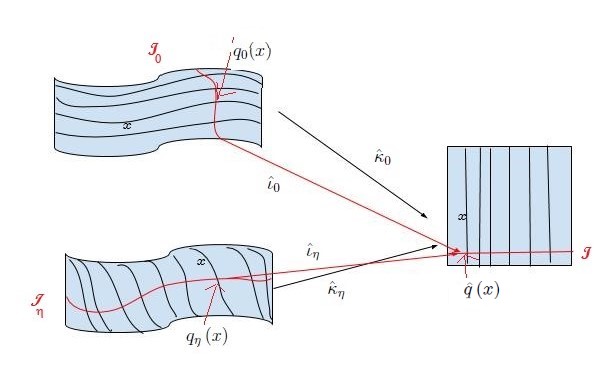
Figure 1: $\hat{\iota}_{0}\circ q_{0}=\hat{q}\circ\hat{\kappa}_{0}\,,\,\hat{\iota}_{\eta}\circ q_{\eta}=\hat{q}\circ\hat{\kappa}_{\eta}.$ Therefore, $\iota_{\eta}:=\hat{\iota}_{\eta}\circ\hat{\iota}_{0}^{-1}\,,\,\kappa_{\eta}:=\hat{\kappa}_{\eta}\circ\hat{\kappa}_{0}^{-1}$ implies $\iota_{\eta}\circ q_{\eta}=q_{0}\circ\kappa_{\eta}.$

5.3 The suspension semi-flow

Let us set

$$\mathcal{M}\backslash\Gamma_{\eta}\ni x\longmapsto\sigma_{\eta}^{n}\left(x\right):=\sum_{k=0}^{n-1}\tau_{\eta}\left(R_{\eta}^{k}\left(x\right)\right)\in\mathbb{R}^{+}\ ,\;n\geq 1\ ,$$ (33)

and, $\forall x\in\mathcal{M}\backslash\Gamma_{\eta},$

$$\mathbb{R}^{+}\ni t\longmapsto n_{\eta}\left(x,t\right):=\max\left\{n\in\mathbb{Z}^{+}:\sigma_{\eta}^{n}\left(x\right)\leq t\right\}\in\mathbb{Z}^{+}\ .$$ (34)

If

$$\mathcal{M}_{\tau_{\eta}}:=\left\{\left(x,s\right)\in\mathcal{M}\times\mathbb{R}^{+}:s\in[0,\tau_{\eta}\left(x\right))\right\}\subset\mathbb{R}^{3}\ ,$$ (35)

we define the suspension semiflow $\left(S_{\eta}^{t},t\geq 0\right)$ as

$$\mathcal{M}_{\tau_{\eta}}\ni\left(x,s\right)\longmapsto S_{\eta}^{t}\left(x,s\right):=\left(R_{\eta}^{n_{\eta}\left(x,t+s\right)}\left(x\right),t+s-\sigma_{\eta}^{n_{\eta}\left(x,s+t\right)}\left(x\right)\right)\in\mathcal{M}_{\tau_{\eta}}\ ,\;t\geq 0\ .$$ (36)

Let $\sim_{\eta}$ be the equivalence relation on $\mathcal{M}\times\mathbb{R}^{+}$ such that any two points $\left(x,s\right),\left(y,t\right)$ in $\mathcal{M}\times\mathbb{R}^{+}$ belong to the same equivalence class if there exist $\left(x_{0},s_{0}\right)\in\mathcal{M}_{\tau_{\eta}},s^{\prime},s^{\prime\prime}>0$ such that $\Phi_{\eta,\tau_{\eta}}^{s^{\prime}}\left(x_{0},s_{0}\right)=\left(x,s\right),\Phi_{\eta,\tau_{\eta}}^{s^{\prime\prime}}\left(x_{0},s_{0}\right)=\left(y,t\right)$ and $n_{\eta}\left(x_{0},s^{\prime\prime}\vee s^{\prime}+s_{0}\right)-n_{\eta}\left(x_{0},s^{\prime\prime}\wedge s^{\prime}+s_{0}\right)\in\mathbb{N}.$ We denote by $\mathcal{V}_{\eta}:=\mathcal{M}\times\mathbb{R}^{+}/\sim_{\eta}$ the corresponding quotient space and by $\tilde{\pi}_{\eta}:\mathcal{M}\times\mathbb{R}^{+}\longrightarrow\mathcal{V}_{\eta}$ the canonical projection which induces a topology and consequently a Borel $\sigma$algebra on $\mathcal{V}_{\eta}.$ Therefore,

$$\mathcal{M}\times\mathbb{R}^{+}\ni\left(x,s\right)\longmapsto S_{\eta}^{t}\circ\tilde{\pi}_{\eta}\left(x,s\right)=\tilde{\pi}_{\eta}\left(x,s+t\right)\in\mathcal{V}_{\eta}\ ,\;t>0\ .$$ (37)

Let us define $\bar{\tau}_{\eta}:\mathcal{M}\backslash\Gamma_{0}\longrightarrow\mathbb{R}^{+}$ such that

$$\bar{\tau}_{\eta}\circ\kappa_{\eta}=\tau_{\eta}\ ,$$ (38)

and consequently

$$\mathcal{M}_{\bar{\tau}_{\eta}}:=\left\{\left(x,s\right)\in\mathcal{M}\times\mathbb{R}^{+}:s\in[0,\bar{\tau}_{\eta}\left(x\right))\right\}\subset\mathbb{R}^{3}\ .$$ (39)

Setting $\bar{\sigma}_{\eta}^{n},n\in\mathbb{Z}^{+},$ and $\bar{n}_{\eta}$ such that

$$\bar{\sigma}_{\eta}^{n}\circ\kappa_{\eta}=\sigma_{\eta}^{n}\;;\;\bar{n}_{\eta}\circ\kappa_{\eta}=n_{\eta}$$ (40)

and

$$\mathcal{M}_{\bar{\tau}_{\eta}}\ni\left(x,s\right)\longmapsto\overline{S}_{\eta}^{t}\left(x,s\right):=\left(\bar{R}_{\eta}^{\bar{n}_{\eta}\left(x,t+s\right)}\left(x\right),t+s-\bar{\sigma}_{\eta}^{\bar{n}_{\eta}\left(x,s+t\right)}\left(x\right)\right)\in\mathcal{M}_{\bar{\tau}_{\eta}}\ ,\;t\geq 0\ ,$$ (41)

we can lift of the diffeomorphism $\kappa_{\eta}$ defined in (23) to the diffeomorphism

$$\mathcal{M}_{\tau_{\eta}}\ni\left(x,s\right)\longmapsto\bar{\kappa}_{\eta}\left(x,s\right):=\left(\kappa_{\eta}\left(x\right),\frac{\bar{\tau}_{\eta}\circ\kappa_{\eta}\left(x\right)}{\tau_{\eta}\left(x\right)}s\right)=\left(\kappa_{\eta}\left(x\right),s\right)\in\mathcal{M}_{\bar{\tau}_{\eta}}\ ,$$ (42)

so that, by (26),

$$\bar{\kappa}_{\eta}\circ S_{\eta}^{t}=\overline{S}_{\eta}^{t}\circ\bar{\kappa}_{\eta}\ .$$ (43)

Let $\approx_{\eta}$ to be the equivalence relation on $\mathcal{M}\times\mathbb{R}^{+}$ such that any two points $\left(x,s\right),\left(y,t\right)$ in $\mathcal{M}\times\mathbb{R}^{+}$ belong to the same equivalence class if there exist $\left(x_{0},s_{0}\right)\in\mathcal{M}_{\bar{\tau}_{\eta}},s^{\prime},s^{\prime\prime}>0$ such that $\bar{\Phi}_{\eta,\bar{\tau}_{\eta}}^{s^{\prime}}\left(x_{0},s_{0}\right)=\left(x,s\right),\bar{\Phi}_{\eta,\bar{\tau}_{\eta}}^{s^{\prime\prime}}\left(x_{0},s_{0}\right)=\left(y,t\right)$ and $\bar{n}_{\eta}\left(x_{0},s^{\prime\prime}\vee s^{\prime}+s_{0}\right)-\bar{n}_{\eta}\left(x_{0},s^{\prime\prime}\wedge s^{\prime}+s_{0}\right)\in\mathbb{N}.$ Denoting by $\overline{\mathcal{V}}_{\eta}:=\mathcal{M}\times\mathbb{R}^{+}/\approx_{\eta}$ the corresponding quotient space and by $\breve{\pi}_{\eta}:\mathcal{M}\times\mathbb{R}^{+}\longrightarrow\overline{\mathcal{V}}_{\eta}$ the canonical projection such that

$$\mathcal{M}\times\mathbb{R}^{+}\ni\left(x,s\right)\longmapsto\overline{S}_{\eta}^{t}\circ\breve{\pi}_{\eta}\left(x,s\right)=\breve{\pi}_{\eta}\left(x,s+t\right)\in\overline{\mathcal{V}}_{\eta}\ ,\;t>0$$ (44)

by (42) we can define a diffeomorphism $\tilde{\kappa}_{\eta}:\mathcal{V}_{\eta}\longrightarrow\overline{\mathcal{V}}_{\eta}$ such that

$$\tilde{\kappa}_{\eta}\circ\tilde{\pi}_{\eta}=\breve{\pi}_{\eta}\circ\tilde{\kappa}_{\eta}\ .$$ (45)

Part II Stochastic stability for impulsive type forcing

As already anticipated in the introduction, in this section we will study the weak convergence of the invariant measure of the semi-Markov random evolution describing the random perturbations of $\left(\Phi_{0}^{t},t\geq 0\right)$ in a neighborhood of the unperturbed attractor to the unperturbed physical measure.

To this purpose we will first consider the RDS defined by the composition of the maps $\bar{R}_{\eta}$ given in (26) which, by construction, preserve the unperturbed invariant foliation. Then, we give an explicit representation for the invariant measure of the original process in terms of the invariant measure for this auxiliary process which, in turn, can be defined starting from the invariant measure for the RDS defined by the composition of the maps $\bar{T}_{\eta}.$

Finally, we will prove that the stochastic stability of the unperturbed physical measure follows from the stochastic stability of the invariant measure for the one-dimensional dynamical system defined by the map $T_{0}.$

6 The associated Random Dynamical System

In this section we present the construction of the auxiliary random processes needed to build up a representation of the random evolution given in (4) in the framework of RDSs. We refer the reader to [Ar] Section 1.1.1 for an account on the definition of a RDS in a more general setup.

6.1 Random maps

1. $$I\times\Omega\ni\left(u,\omega\right)\longmapsto\mathbf{T}\left(u,\omega\right):=\left(\bar{T}_{\pi\left(\omega\right)}\left(u\right),\theta\omega\right)\in I\times\Omega\ ,$$ (46)

   with $\mathbf{T}^{0}$ the identity operator on $I\times\Omega,$ defines a measurable random dynamical system on $\left(I,\mathcal{B}\left(I\right)\right)$ over the metric dynamical system $\left(\Omega,\mathcal{F},\mathbb{P},\theta\right);$

2. setting $\mathcal{\tilde{M}}:=\mathcal{M}\backslash\Gamma_{0},$

   $$\mathcal{\tilde{M}}\times\Omega\ni\left(x,\omega\right)\longmapsto\overline{\mathbf{R}}\left(x,\omega\right)\in\left(\bar{R}_{\pi\left(\omega\right)}\left(x\right),\theta\omega\right)\in\mathcal{M}\times\Omega\ ,$$ (47)

   with $\overline{\mathbf{R}}^{0}$ the identity operator on $\mathcal{M}\times\Omega,$ define two measurable random dynamical systems on $\left(\mathcal{M},\mathcal{B}\left(\mathcal{M}\right)\right)$ over the metric dynamical system $\left(\Omega,\mathcal{F},\mathbb{P},\theta\right).$

   Let

   $$\mathcal{M}\times\Omega\ni\left(x,\omega\right)\longmapsto Q\left(x,\omega\right):=\left(q\left(x\right),\omega\right)\in I\times\Omega\ .$$ (48)

   Then, $\forall\left(x,\omega\right)\in\mathcal{\tilde{M}}\times\Omega,$

   $$\left(Q\circ\overline{\mathbf{R}}\right)\left(x,\omega\right) =Q\left(\bar{R}_{\pi\left(\omega\right)}\left(x\right),\theta\omega\right)=\left(q\left(\bar{R}_{\pi\left(\omega\right)}\left(x\right)\right),\theta\omega\right)$$ (49)

   $$=\left(\bar{T}_{\pi\left(\omega\right)}\left(q\left(x\right)\right),\theta\omega\right)=\left(\mathbf{T}\circ Q\right)\left(x,\omega\right)$$

   that is

   $$Q\circ\overline{\mathbf{R}}=\mathbf{T}\circ Q\ .$$ (50)

   Defining the map

   $$\mathcal{M}\times\Omega\ni\left(x,\omega\right)\longmapsto\mathbf{K}\left(x,\omega\right):=\left(\kappa_{\pi\left(\omega\right)}\left(x\right),\omega\right)\in\mathcal{M}\times\Omega\ ,$$ (51)

   for any $\left(x,\omega\right)\in\widetilde{\mathcal{M}\times\Omega}:=\left(\mathcal{M}\times\Omega\right)\backslash\left\{\left(x,\omega\right)\in\mathcal{M}\times\Omega:x\in\Gamma_{\pi\left(\omega\right)}\right\},$ we define $\mathbf{R}:\widetilde{\mathcal{M}\times\Omega}\longrightarrow\mathcal{M}\times\Omega$ such that

   $$\overline{\mathbf{R}}\circ\mathbf{K}\left(x,\omega\right)=\mathbf{K}\left(x,\omega\right)\circ\mathbf{R}\ ,$$ (52)

   that is

   $$\widetilde{\mathcal{M}\times\Omega}\ni\left(x,\omega\right)\longmapsto\left(\bar{R}_{\pi\left(\omega\right)}\left(x\right)\circ\kappa_{\pi\left(\omega\right)},\theta\omega\right)=\left(\kappa_{\pi\left(\omega\right)}\circ R_{\pi\left(\omega\right)}\left(x\right),\theta\omega\right)\in\mathcal{M}\times\Omega\ .$$ (53)

6.2 The random suspension semi-flow

Let

$$\mathcal{M}\times\Omega\ni\left(x,\omega\right)\longmapsto\mathbf{t}\left(x,\omega\right):=\tau_{\pi\left(\omega\right)}\left(x\right)\in\overline{\mathbb{R}^{+}}\ .$$ (54)

Then, $\forall n\geq 1,$ we define

$$\mathcal{M}\times\Omega\ni\left(x,\omega\right)\longmapsto\mathbf{s}_{n}\left(x,\omega\right):=\sum_{k=0}^{n-1}\mathbf{t}\left(\mathbf{R}^{k}\left(x,\omega\right)\right)\in\overline{\mathbb{R}^{+}}\ ,\;n\geq 1\ ,$$ (55)

and denote, $\forall t>0,$

$$\mathcal{M}\times\Omega\ni\left(x,\omega\right)\longmapsto N_{t}\left(x,\omega\right):=\max\left\{n\in\mathbb{Z}^{+}:\mathbf{s}_{n}\left(x,\omega\right)\leq t\right\}\in\mathbb{Z}^{+}\mathbb{\ }.$$ (56)

We now proceed as in the definition of standard suspension flow given in (36). We define

$$\left(\mathcal{M}\times\Omega\right)_{\mathbf{t}}:=\left\{\left(x,\omega,s\right)\in\widetilde{\mathcal{M}\times\Omega}\times\mathbb{R}^{+}:s\in[0,\mathbf{t}\left(x,\omega\right))\right\}$$ (57)

and consequently the semiflow $\left(\mathbf{S}^{t},t\geq 0\right),$ which we will call random suspension semi-flow, where

$$\left(\mathcal{M}\times\Omega\right)_{\mathbf{t}}\ni\left(x,\omega,s\right)\longmapsto\mathbf{S}^{t}\left(x,\omega,s\right):=\left(\mathbf{R}^{N_{s+t}\left(x,\omega\right)}\left(x,\omega\right),s+t-\mathbf{s}_{N_{s+t}\left(x,\omega\right)}\left(x,\omega\right)\right)\in\left(\mathcal{M}\times\Omega\right)_{\mathbf{t}}\ .$$ (58)

Let $\sim$ be the equivalence relation on $\mathcal{M}\times\Omega\times\mathbb{R}^{+}$ such that any two points $\left(x,\omega,s\right),\left(y,\omega^{\prime},t\right)$ in $\mathcal{M}\times\Omega\times\mathbb{R}^{+}$ belong to the same equivalence class if there exist $\left(x_{0},\omega_{0},s_{0}\right)\in\left(\mathcal{M}\times\Omega\right)_{\mathbf{t}}$ and $t^{\prime},t^{\prime\prime}>0$ such that $\mathbf{S}^{t^{\prime}}\left(x_{0},\omega_{0},s_{0}\right)=\left(x,\omega,s\right),\mathbf{S}^{t^{\prime\prime}}\left(x_{0},\omega_{0},s_{0}\right)=\left(y,\omega^{\prime},t\right)$ and $N_{t^{\prime\prime}\vee t^{\prime}+s_{0}}\left(x_{0},\omega_{0}\right)-N_{t^{\prime\prime}\wedge t^{\prime}+s_{0}}\left(x_{0},\omega_{0}\right)\in\mathbb{N}.$ We denote by $\mathfrak{V}:=\mathcal{M}\times\Omega\times\mathbb{R}^{+}/\sim$ the corresponding quotient space and by $\hat{\pi}:\mathcal{M}\times\Omega\times\mathbb{R}^{+}\longrightarrow\mathfrak{V}$ the canonical projection which induces a topology and consequently a Borel $\sigma$algebra on $\mathfrak{V}.$ Therefore,

$$\mathcal{M}\times\Omega\times\mathbb{R}^{+}\ni\left(x,\omega,s\right)\longmapsto\mathbf{S}^{t}\circ\hat{\pi}\left(x,\omega,s\right)=\hat{\pi}\left(x,\omega,s+t\right)\in\mathfrak{V}\ ,\;t>0\ .$$ (59)

Let us define $\mathbf{\bar{t}}:\widetilde{\mathcal{M}\times\Omega}\longrightarrow\mathbb{R}^{+}$ such that

$$\mathbf{\bar{t}}\circ\mathbf{K}=\mathbf{t}$$ (60)

and consequently

$$\left(\mathcal{M}\times\Omega\right)_{\mathbf{\bar{t}}}:=\left\{\left(x,\omega,s\right)\in\mathcal{M}\times\Omega\times\mathbb{R}^{+}:s\in[0,\mathbf{\bar{t}}\left(x,\omega\right))\right\}\ .$$ (61)

Setting $\mathbf{\bar{s}}_{n},n\in\mathbb{N}$ and $\overline{N}$ such that

$$\mathbf{\bar{s}}_{n}\circ\mathbf{K=s}_{n}\;;\;\overline{N}\circ\mathbf{K}=N$$ (62)

and

$$\left(\mathcal{M}\times\Omega\right)_{\mathbf{t}}\ni\left(x,\omega,s\right)\longmapsto\overline{\mathbf{S}}^{t}\left(x,\omega,s\right):=\left(\overline{\mathbf{R}}^{\overline{N}_{s+t}\left(x,\omega\right)}\left(x,\omega\right),s+t-\mathbf{\bar{s}}_{\overline{N}_{s+t}\left(x,\omega\right)}\left(x,\omega\right)\right)\in\left(\mathcal{M}\times\Omega\right)_{\mathbf{\bar{t}}}\ ,$$ (63)

we can lift the map defined in (51), as we did to get (42), to the map

$$\left(\mathcal{M}\times\Omega\right)_{\mathbf{t}}\ni\left(x,\omega,s\right)\longmapsto\overline{\mathbf{K}}\left(x,\omega,s\right):=\left(\mathbf{K}\left(x,\omega\right),s\right)\in\left(\mathcal{M}\times\Omega\right)_{\mathbf{\bar{t}}}$$ (64)

so that

$$\overline{\mathbf{K}}\circ\mathbf{S}^{t}=\overline{\mathbf{S}}^{t}\circ\overline{\mathbf{K}}\ .$$ (65)

Let $\approx$ be the equivalence relation on $\mathcal{M}\times\Omega\times\mathbb{R}^{+}$ such that any two points $\left(x,\omega,s\right),\left(y,\omega^{\prime},t\right)$ in $\mathcal{M}\times\Omega\times\mathbb{R}^{+}$ belong to the same equivalence class if there exist $\left(x_{0},\omega_{0},s_{0}\right)\in\left(\mathcal{M}\times\Omega\right)_{\mathbf{\bar{t}}}$ and $t^{\prime},t^{\prime\prime}>0$ such that $\overline{\mathbf{S}}^{t^{\prime}}\left(x_{0},\omega_{0},s_{0}\right)=\left(x,\omega,s\right),\overline{\mathbf{S}}^{t^{\prime\prime}}\left(x_{0},\omega_{0},s_{0}\right)=\left(y,\omega^{\prime},t\right)$ and $\overline{N}_{t^{\prime\prime}\vee t^{\prime}+s_{0}}\left(x_{0},\omega_{0}\right)-\overline{N}_{t^{\prime\prime}\wedge t^{\prime}+s_{0}}\left(x_{0},\omega_{0}\right)\in\mathbb{N}.$ We denote by $\overline{\mathfrak{V}}:=\mathcal{M}\times\Omega\times\mathbb{R}^{+}/\approx$ the corresponding quotient space and by $\check{\pi}:\mathcal{M}\times\Omega\times\mathbb{R}^{+}\longrightarrow\overline{\mathfrak{V}}$ the canonical projection such that

$$\mathcal{M}\times\Omega\times\mathbb{R}^{+}\ni\left(x,\omega,s\right)\longmapsto\overline{\mathbf{S}}^{t}\circ\check{\pi}\left(x,\omega,s\right)=\check{\pi}\left(x,\omega,s+t\right)\in\overline{\mathfrak{V}}\ ,\;t>0\ ,$$ (66)

by (64) we can define a map $\mathbf{\tilde{K}}:\mathfrak{V}\longrightarrow\overline{\mathfrak{V}}$ such that

$$\mathbf{\tilde{K}}\circ\hat{\pi}=\check{\pi}\circ\mathbf{\tilde{K}\ .}$$ (67)

7 The invariant measures

7.1 The invariant measure for the RDS’s $\overline{\mathbf{R}}$ and $\mathbf{R}$ on $\left(\mathcal{M},\mathcal{B}\left(\mathcal{M}\right)\right)$

Let us assume $\mu_{\mathbf{T}}\in\mathfrak{I}_{\mathbb{P}}\left(\mathbf{T}\right)$ to be the invariant measure for $\mathbf{T.}$

The results in [AP] Section 7.3.4.1 applies almost verbatim to $\mathbf{T}$ and $\overline{\mathbf{R}}$ (see in particular Lemma 7.21 and Corollary 7.22). Hence the proof of the following result is deferred to the appendix.

Proposition 2

Let $\mu_{\mathbf{T}}$ be the invariant measure for $\mathbf{T}.$ There exists a measure $\mu_{\overline{\mathbf{R}}}$ on $\left(\mathcal{M}\times\Omega,\mathcal{B}\left(\mathcal{M}\right)\otimes\mathcal{F}\right),$ invariant under $\overline{\mathbf{R}},$ such that, $\forall\psi\in L_{\mathbb{P}}^{1}\left(\Omega,C_{b}\left(\mathcal{M}\right)\right),$

$$\mu_{\overline{\mathbf{R}}}\left(\psi\right):=\lim_{n\rightarrow\infty}\int\mu_{\mathbf{T}}\left(du,d\omega\right)\inf_{x\in q^{-1}\left(u\right)}\psi\circ\overline{\mathbf{R}}^{n}\left(x,\omega\right)$$ (68)

and the correspondence $\mu_{\mathbf{T}}\longmapsto\mu_{\overline{\mathbf{R}}}$ is injective. Moreover, if $\mu_{\mathbf{T}}$ is ergodic, then $\mu_{\overline{\mathbf{R}}}$ is also ergodic.

Remark 3

If $\mu_{\mathbf{T}}\in\mathfrak{I}_{\mathbb{P}}\left(\mathbf{T}\right)$ then $\mu_{\overline{\mathbf{R}}}\in\mathfrak{I}_{\mathbb{P}}\left(\overline{\mathbf{R}}\right)$ and, by [Ar] Proposition 1.4.3, the correspondence $\mu_{\mathbf{T}}\left(\cdot|\omega\right)\longmapsto\mu_{\overline{\mathbf{R}}}\left(\cdot|\omega\right)$ is injective.

Moreover, if $\mu_{\mathbf{T}}$ admits the disintegration $\mu_{\mathbf{T}}\left(du,d\omega\right)=\nu_{1}\left(du\right)\mathbb{P}\left(d\omega\right),$ by [Ar] Theorem 2.1.7, $\nu_{1}$ is the stationary measure for the Markov chain with transition operator

$$C_{b}\left(I\right)\ni\varphi\longmapsto P_{T}\varphi:=\mathbb{E}\left[\varphi\circ\mathbf{q}\circ\mathbf{T}\right]\in M_{b}\left(I\right)\ ,$$ (69)

where

$$I\times\Omega\ni\left(u,\omega\right)\longmapsto\mathbf{q}\left(u,\omega\right):=u\in I\ .$$ (70)

Therefore, there exists a stationary measure $\mu_{\overline{\mathbf{R}}}$ for the Markov chain with transition operator

$$C_{b}\left(\mathcal{M}\right)\ni\psi\longmapsto P_{\overline{R}}\psi:=\mathbb{E}\left[\psi\circ p\circ\overline{\mathbf{R}}\right]\in M_{b}\left(\mathcal{M}\right)\ ,$$ (71)

such that $\mu_{\overline{\mathbf{R}}}=\bar{\nu}_{2}\otimes\mathbb{P}.$ Indeed, by (68),

$$\bar{\nu}_{2}\left(\psi\right) =\lim_{n\longrightarrow\infty}\int\nu_{1}\left(du\right)\mathbb{E}\left[\inf_{x\in q^{-1}\left(u\right)}\left[\psi\circ p\circ\overline{\mathbf{R}}^{n}\right]\left(x,\cdot\right)\right]$$ (72)

$$=\lim_{n\longrightarrow\infty}\int\nu_{1}\left(du\right)\inf_{x\in q^{-1}\left(u\right)}\left(P_{\overline{R}}^{n}\psi\right)\left(x\right)$$

and, by (230),

$$\bar{\nu}_{2}\left(P_{\overline{R}}\psi\right) =\lim_{n\longrightarrow\infty}\int\nu_{1}\left(du\right)\inf_{x\in q^{-1}\left(u\right)}\left(P_{\overline{R}}^{n+1}\psi\right)\left(x\right)$$ (73)

$$=\lim_{n\longrightarrow\infty}\int\nu_{1}\left(du\right)\mathbb{E}\left[\inf_{x\in q^{-1}\left(u\right)}\left[\psi\circ p\circ\overline{\mathbf{R}}^{n+1}\right]\left(x,\cdot\right)\right]=\bar{\nu}_{2}\left(\psi\right)\ .$$

Moreover, for any $\varphi\in C_{b}\left(I\right),\varphi\circ q\in C_{b}\left(\mathcal{M}\right);$ thus, by (50),

$$\bar{\nu}_{2}\left(\varphi\circ q\right) =\lim_{n\longrightarrow\infty}\int\nu_{1}\left(du\right)\mathbb{E}\left[\inf_{x\in q^{-1}\left(u\right)}\left[\varphi\circ q\circ p\circ\overline{\mathbf{R}}^{n}\right]\left(x,\cdot\right)\right]$$ (74)

$$=\lim_{n\longrightarrow\infty}\int\nu_{1}\left(du\right)\mathbb{E}\left[\inf_{x\in q^{-1}\left(u\right)}\left[\varphi\circ\mathbf{q}\circ Q\circ\overline{\mathbf{R}}^{n}\right]\left(x,\cdot\right)\right]$$

$$=\lim_{n\longrightarrow\infty}\int\nu_{1}\left(du\right)\mathbb{E}\left[\inf_{x\in q^{-1}\left(u\right)}\left[\varphi\circ\mathbf{q}\circ\mathbf{T}^{n}\circ Q\right]\left(x,\cdot\right)\right]$$

$$=\lim_{n\longrightarrow\infty}\int\nu_{1}\left(du\right)\mathbb{E}\left[\left[\varphi\circ\mathbf{q}\circ\mathbf{T}^{n}\right]\left(u,\cdot\right)\right]$$

$$=\lim_{n\longrightarrow\infty}\int\nu_{1}\left(du\right)P_{T}^{n}\varphi\left(u\right)=\nu_{1}\left[\varphi\right]\ .$$

Since $\mathcal{B}_{I}:=q^{-1}\left(\mathcal{B}\left(I\right)\right)$ is a sub-$\sigma$algebra of $\mathcal{B}\left(\mathcal{M}\right)$ and since $\bar{\nu}_{2}\left(\varphi|\mathcal{B}_{I}\right)$ is constant on the leaves of the invariant foliation, we get $\bar{\nu}_{2}\left(\varphi\right)=\bar{\nu}_{2}\left(\bar{\nu}_{2}\left(\varphi|\mathcal{B}_{I}\right)\right)=\nu_{1}\left[\bar{\nu}_{2}\left(\varphi|\mathcal{B}_{I}\right)\right].$ Hence, since by definition $\forall u\in I,\omega\in\Omega,$

$$\lim_{n\rightarrow\infty}\operatorname*{diam}p\left(\overline{\mathbf{R}}^{n}\left(Q^{-1}\left(u,\omega\right)\right)\right)=0\ ,$$ (75)

$\bar{\nu}_{2}$ is singular w.r.t. the Lebesgue measure on $\left(\mathcal{M},\mathcal{B}\left(\mathcal{M}\right)\right),$ while the marginal of $\bar{\nu}_{2}$ on $\left(I,\mathcal{B}\left(I\right)\right)$ coincides with $\nu_{1}.$

Corollary 4

If $\mu_{\overline{\mathbf{R}}}\in\mathfrak{I}_{\mathbb{P}}\left(\overline{\mathbf{R}}\right)$ then $\mu_{\mathbf{R}}:=\mathbf{K}_{\#}^{-1}\mu_{\overline{\mathbf{R}}}=\mu_{\overline{\mathbf{R}}}\circ\mathbf{K}\in\mathfrak{I}_{\mathbb{P}}\left(\mathbf{R}\right),$ with, by (52),

$$\mathcal{M}\times\Omega\ni\left(x,\omega\right)\longmapsto\mathbf{K}^{-1}\left(x,\omega\right):=\left(\kappa_{\pi\left(\omega\right)}^{-1}\left(x\right),\omega\right)\in\mathcal{M}\times\Omega\ .$$ (76)

Proof. By (52), for any $A\in\mathcal{B}\left(\mathcal{M}\right)\otimes\mathcal{F}$ we get

$$\mu_{\mathbf{R}}\left(\mathbf{R}^{-1}\left(A\right)\right) =\mu_{\overline{\mathbf{R}}}\circ\mathbf{K}\left(\mathbf{R}^{-1}\left(A\right)\right)=\mu_{\overline{\mathbf{R}}}\circ\mathbf{K}\left(\left(\mathbf{R}^{-1}\circ\mathbf{K}^{-1}\right)\left(\mathbf{K}\left(A\right)\right)\right)$$ (77)

$$=\mu_{\overline{\mathbf{R}}}\circ\mathbf{K}\left(\left(\mathbf{K}^{-1}\circ\overline{\mathbf{R}}^{-1}\right)\left(\mathbf{K}\left(A\right)\right)\right)=\mu_{\overline{\mathbf{R}}}\left(\overline{\mathbf{R}}^{-1}\left(\mathbf{K}\left(A\right)\right)\right)=\mu_{\overline{\mathbf{R}}}\circ\mathbf{K}\left(A\right)\ .$$

 

7.2 The invariant measure for the random semi-flow $\left(\mathbf{S}^{t},t\geq 0\right)$

Lemmata 7.28 and 7.29 as well as Corollary 7.30 in Section 7.3.6 of [AP] applies verbatim to the semi-flow (63). We summarize these statements in the following Lemma.

Lemma 5

Assume that the return time $\mathbf{\bar{t}}$ in (54) is bounded away from zero and integrable w.r.t. $\mu_{\overline{\mathbf{R}}}.$ Then the measure on $\left(\overline{\mathfrak{V}},\mathcal{B}\left(\overline{\mathfrak{V}}\right)\right)$ such that, for any bounded measurable function $f:\overline{\mathfrak{V}}\longrightarrow\mathbb{R},$

$$\mu_{\overline{\mathbf{S}}}\left(f\right):=\frac{1}{\mu_{\overline{\mathbf{R}}}\left(\mathbf{\bar{t}}\right)}\int\mu_{\overline{\mathbf{R}}}\left(dx,d\omega\right)\int_{0}^{\mathbf{\bar{t}}\left(x,\omega\right)}dtf\circ\check{\pi}\left(x,\omega,t\right)$$ (78)

is invariant under the semi-flow defined by (66) on $\overline{\mathfrak{V}}.$

Moreover, the correspondence $\mu_{\overline{\mathbf{R}}}\longmapsto\mu_{\overline{\mathbf{S}}}$ (and so $\mu_{\mathbf{T}}\longmapsto\mu_{\overline{\mathbf{R}}}\longmapsto\mu_{\overline{\mathbf{S}}}$) is injective.

Furthermore, if $\mu_{\overline{\mathbf{R}}}$ is invariant under $\overline{\mathbf{R}},$ then

$$\lim_{T\longrightarrow\infty}\frac{1}{T}\int_{0}^{T}dtf\circ\check{\pi}\left(x,\omega,t\right)=\mu_{\overline{\mathbf{S}}}\left(f\right)\ .$$ (79)

As a byproduct, if $\mu_{\overline{\mathbf{R}}}$ is ergodic $\mu_{\overline{\mathbf{S}}}$ is also ergodic.

Proof. The proof of the invariance of $\mu_{\overline{\mathbf{S}}}$ under $\left(\overline{\mathbf{S}}^{t},t\geq 0\right)$ on $\overline{\mathfrak{V}}$ follows word by word that of Lemma 7.28 in Section 7.3.6 of [AP]. The injectivity of the correspondence $\mu_{\overline{\mathbf{R}}}\longmapsto\mu_{\overline{\mathbf{S}}}$ follows from that of the correspondence $\psi\longmapsto f$ associating to any bounded measurable function $\psi:\mathcal{M}\times\Omega\longrightarrow\mathbb{R}$ the bounded measurable function

$$\mathfrak{V}\ni\left(x,\omega,t\right)\longmapsto f\left(x,\omega,t\right):=\mu_{\overline{\mathbf{R}}}\left(\mathbf{\bar{t}}\right)\frac{\psi\left(x,\omega\right)}{\mathbf{\bar{t}}\left(x,\omega\right)}\mathbf{1}_{[0,\mathbf{\bar{t}}\left(x,\omega\right))}\left(t\right)\in\mathbb{R}$$ (80)

such that $\mu_{\overline{\mathbf{S}}}\left(f\right)=\mu_{\overline{\mathbf{R}}}\left(\psi\right).$ The proof of the last result as well as ergodicity of $\mu_{\overline{\mathbf{S}}}$ under the hypothesis of ergodicity of $\mu_{\overline{\mathbf{R}}}$ are identical respectively to that of Lemma 7.28 and Corollary 7.30 in Section 7.3.6 of [AP].   

Proposition 6

Under the hypothesis of the preceding lemma, the measure on $\left(\mathfrak{V},\mathcal{B}\left(\mathfrak{V}\right)\right)$ such that, for any bounded measurable function $f:\mathfrak{V}\longrightarrow\mathbb{R},$

$$\mu_{\mathbf{S}}\left(f\right):=\frac{1}{\mu_{\mathbf{R}}\left(\mathbf{t}\right)}\int\mu_{\mathbf{R}}\left(dx,d\omega\right)\int_{0}^{\mathbf{t}\left(x,\omega\right)}dtf\circ\hat{\pi}\left(x,\omega,t\right)$$ (81)

is invariant under the semi-flow defined by (59) on $\mathfrak{V}.$

Moreover, the correspondence $\mu_{\mathbf{T}}\longmapsto\mu_{\mathbf{R}}\longmapsto\mu_{\mathbf{S}}$) is injective.

Furthermore, if $\mu_{\overline{\mathbf{R}}}$ is invariant under $\overline{\mathbf{R}},$ then

$$\lim_{T\longrightarrow\infty}\frac{1}{T}\int_{0}^{T}dtf\circ\hat{\pi}\left(x,\omega,t\right)=\mu_{\mathbf{S}}\left(f\right)\ .$$ (82)

As a byproduct, if $\mu_{\overline{\mathbf{R}}}$ is ergodic $\mu_{\mathbf{S}}$ is also ergodic.

Proof. If $\mathbf{t}\in L_{\mu_{\mathbf{R}}}^{1}$the proof of the invariance of $\mu_{\mathbf{S}}$ under $\left(\mathbf{S}^{t},t\geq 0\right)$ on $\mathfrak{V}$ is identical to that given in the previous lemma. Moreover, the proof of the ergodicity of $\mu_{\mathbf{S}}$ under the hypothesis of ergodicity of $\mu_{\mathbf{R}}$ follows the same lines of that of the corresponing statements involving $\mu_{\overline{\mathbf{S}}}$ and $\mu_{\overline{\mathbf{R}}}$ in view of the previous corollary and the fact that, by (60),

$$\mu_{\overline{\mathbf{R}}}\left(\mathbf{\bar{t}}\right)=\mathbf{K}_{\#}\mu_{\mathbf{R}}\left(\mathbf{\bar{t}}\right)=\mu_{\mathbf{R}}\left(\mathbf{\bar{t}}\circ\mathbf{K}\right)=\mu_{\mathbf{R}}\left(\mathbf{t}\right)\ ,$$ (83)

which, by (67), $\forall f:\overline{\mathfrak{V}}\longrightarrow\mathbb{R},$ imply

$$\mu_{\overline{\mathbf{S}}}\left(f\right) =\mathbf{\tilde{K}}_{\#}\mu_{\mathbf{S}}\left(f\right)=\mu_{\mathbf{S}}\left(f\circ\mathbf{\tilde{K}}\right)=\frac{1}{\mu_{\mathbf{R}}\left(\mathbf{t}\right)}\mu_{\mathbf{R}}\otimes\lambda\left[\mathbf{1}_{\left[0,\mathbf{t}\right]}f\circ\mathbf{\tilde{K}}\circ\hat{\pi}\right]$$ (84)

$$=\frac{1}{\mu_{\overline{\mathbf{R}}}\left(\mathbf{\bar{t}}\right)}\mu_{\mathbf{R}}\otimes\lambda\left[\mathbf{1}_{\left[0,\mathbf{\bar{t}}\circ\mathbf{K}\right]}f\circ\check{\pi}\circ\mathbf{\tilde{K}}\right]$$

$$=\frac{1}{\mu_{\overline{\mathbf{R}}}\left(\mathbf{\bar{t}}\right)}\int\mu_{\mathbf{R}}\left(dx,d\omega\right)\int_{0}^{\left(\mathbf{\bar{t}}\circ\mathbf{K}\right)\left(x,\omega\right)}dtf\circ\check{\pi}\left(\mathbf{K}\left(x,\omega\right),s\right)$$

i.e., since $\mu_{\overline{\mathbf{R}}}=\mathbf{K}_{\#}\mu_{\mathbf{R}},$ the r.h.s. of (78). Then, the injectivity of the correspondence $\mu_{\mathbf{T}}\longmapsto\mu_{\mathbf{R}}\longmapsto\mu_{\mathbf{S}}$ readily follows.   

By the assumption we made on $\phi_{\eta},$ it has been proven in [AMV] Lemma 2.1 (see also [HM] Proposition 2.6.) that there exists a positive constant $C_{1}$ such that, for any $x\in\mathcal{M},$

$$\bar{\tau}_{\eta}\left(x\right)\leq C_{1}\log\frac{1}{\left|q\left(x\right)-\hat{u}_{0}\right|}\ ,$$ (85)

where $\hat{u}_{0}$ is the image under $q$ of the intersection of $\mathcal{M}$ with the stable manifold of the hyperbolic fixed point. For example, by what stated in Section 12, $\hat{u}_{0}$ equal to $0$ if $\mathcal{M}=\mathcal{M}^{\prime}$ or $\left|\hat{u}_{0}\right|\in\left(0,1\right)$ if $\mathcal{M}=\mathcal{M}^{\prime\prime}.$ The integrability of $\mathbf{\bar{t}}$ w.r.t. $\mu_{\overline{\mathbf{R}}}$ then readily follows.

Lemma 7

If $\mu_{\mathbf{T}}$ is a.c. w.r.t. $\lambda\otimes\mathbb{P}_{\varepsilon}$ with density bounded $\lambda\otimes\mathbb{P}_{\varepsilon}$-a.s., then $\mathbf{\bar{t}}$ is integrable w.r.t. $\mu_{\overline{\mathbf{R}}}.$

Proof. The proof is analogous to that of Lemma 3.7 in [BR]. The sequence $\left\{\mathbf{\bar{t}}^{M}\right\}_{M\in\mathbb{N}}$ such that $\mathbf{\bar{t}}^{M}:=\mathbf{\bar{t}}\wedge M$ is monotone increasing an converging $\mu_{\overline{\mathbf{R}}}$-a.s. to $\mathbf{\bar{t}.}$ So for the monotone convergence theorem is enough to prove that $\mu_{\overline{\mathbf{R}}}\left(\mathbf{\bar{t}}^{M}\right)$ is uniformly bounded in $M.$ By (2),(54) and (60) we get

$$\mu_{\overline{\mathbf{R}}}\left(\mathbf{\bar{t}}^{M}\right) =\underline{\lim}_{n}\int\mu_{\mathbf{T}}\left(du,d\omega\right)\sup_{x\in q^{-1}\left(u\right)}\mathbf{\bar{t}}^{M}\circ\overline{\mathbf{R}}^{n}\left(x,\omega\right)=\lim_{n\rightarrow\infty}\int\mu_{\mathbf{T}}\left(du,d\omega\right)\sup_{\left(x,\omega^{\prime}\right)\in Q^{-1}\left(u,\omega\right)}\mathbf{\bar{t}}^{M}\circ\overline{\mathbf{R}}^{n}\left(x,\omega^{\prime}\right)$$ (86)

$$\leq\lim_{n\rightarrow\infty}\int\mu_{\mathbf{T}}\left(du,d\omega\right)\sup_{\left(x,\omega^{\prime}\right)\in\left\{\left(y,\omega^{\prime\prime}\right)\in\mathcal{M}\times\Omega\ :\ Q\left(y,\omega^{\prime\prime}\right)=\mathbf{T}^{n}\left(u,\omega\right)\right\}}\mathbf{\bar{t}}^{M}\left(x,\omega^{\prime}\right)$$

$$=\int\mu_{\mathbf{T}}\left(du,d\omega\right)\sup_{\left(x,\omega^{\prime}\right)\in Q^{-1}\left(u,\omega\right)}\mathbf{\bar{t}}^{M}\left(x,\omega^{\prime}\right)\leq\int\mu_{\mathbf{T}}\left(du,d\omega\right)\sup_{x\in q^{-1}\left(u\right)}\bar{\tau}_{\pi\left(\omega\right)}\left(x\right)\wedge M$$

$$\leq\left\|\frac{d\mu_{\mathbf{T}}}{d\left(\lambda\otimes\mathbb{P}_{\varepsilon}\right)}\right\|_{\infty}C_{1}\int_{I}du\log\left|u-\hat{u}_{0}\right|<\infty\ .$$

 

8 Stochastic stability

Given $\eta\in spt\lambda_{\varepsilon},$ let $\bar{\eta}\in\Omega$ be such that $\forall m\geq 0,\pi\left(\theta^{m}\bar{\eta}\right)=\eta.$

If $\mu_{\bar{T}_{\eta}}$ denotes the measure on $\left(I,\mathcal{B}\left(I\right)\right)$ invariant under the dynamics defined by the map $\bar{T}_{\eta}$ given in (25), we can lift the metric dynamical system $\left(I,\mathcal{B}\left(I\right),\mu_{T_{\eta}},\bar{T}_{\eta}\right)$ to the metric dynamical system $\left(I\times\Omega,\mathcal{B}\left(I\right)\otimes\mathcal{F},\mu_{\mathbf{T}_{\eta}},\mathbf{T}_{\eta}\right),$ where

$$I\times\Omega\ni\left(u,\omega\right)\longmapsto\mathbf{T}_{\eta}\left(u,\omega\right):=\left(\bar{T}_{\eta}\left(u\right),\theta\omega\right)\in I\times\Omega$$ (87)

and $\mu_{\mathbf{T}_{\eta}}:=\mu_{\bar{T}_{\eta}}\otimes\delta_{\bar{\eta}},$ with $\delta_{\bar{\eta}}$ the Dirac mass at $\bar{\eta}.$

In the same fashion, denoting by $\mu_{R_{\eta}}$ the measure on $\left(\mathcal{M},\mathcal{B}\left(\mathcal{M}\right)\right)$ invariant under the dynamics defined by the map $R_{\eta}$ given in (20), we define the metric dynamical system $\left(\mathcal{M}\times\Omega,\mathcal{B}\left(\mathcal{M}\right)\otimes\mathcal{F},\mu_{\mathbf{R}_{\eta}},\mathbf{R}_{\eta}\right),$ where

$$\left(\mathcal{M}\backslash\Gamma_{\eta}\right)\times\Omega\ni\left(x,\omega\right)\longmapsto\mathbf{R}_{\eta}\left(x,\omega\right)\in\left(R_{\eta}\left(x\right),\theta\omega\right)\in\mathcal{M}\times\Omega$$ (88)

and $\mu_{\mathbf{R}_{\eta}}:=\mu_{R_{\eta}}\otimes\delta_{\bar{\eta}}.$

Moreover, setting

$$\left(\mathcal{M}\backslash\Gamma_{\eta}\right)\times\Omega\ni\left(x,\omega\right)\longmapsto\mathbf{t}_{\eta}\left(x,\omega\right):=\mathbf{t}\left(x,\bar{\eta}\right)=\tau_{\eta}\left(x\right)\in\mathbb{R}^{+}\ ,$$ (89)

we define semi-flow $\left(\mathbf{S}_{\eta}^{t},t\geq 0\right)$ on $\left(\mathcal{M}\times\Omega\right)_{\mathbf{t}_{\eta}}=\mathcal{M}_{\tau_{\eta}}\times\Omega$ as in (58) and consequently, setting

$$\mathcal{M}\times\Omega\times\mathbb{R}^{+}\ni\left(x,\omega,s\right)\longmapsto\hat{\pi}_{\eta}\left(x,\omega,s\right):=\left(\tilde{\pi}_{\eta}\left(x,s\right),\omega\right)\in\mathcal{V}_{\eta}\times\Omega\ ,$$ (90)

the semi-flow

$$\mathcal{M}\times\Omega\times\mathbb{R}^{+}\ni\left(x,\omega,s\right)\longmapsto\mathbf{S}_{\eta}^{t}\circ\hat{\pi}_{\eta}\left(x,\omega,s\right)=\hat{\pi}_{\eta}\left(x,\omega,s+t\right)\in\mathcal{V}_{\eta}\times\Omega\ ,\;t>0\ ,$$ (91)

as in (59). Furthermore, we denote by $\mu_{\mathbf{S}_{\eta}}:=\mu_{S_{\eta}}\otimes\delta_{\bar{\eta}},$ where $\mu_{S_{\eta}}\left(dt,dx\right):=\frac{\mathbf{1}_{\left[0,\tau_{\eta}\left(x\right)\right]}\left(t\right)\mu_{R_{\eta}}\left(dx\right)}{\mu_{R_{\eta}\left(\tau_{\eta}\right)}},$ the measure on $\left(\mathcal{V}_{\eta}\times\Omega,\mathcal{B}\left(\mathcal{V}_{\eta}\right)\otimes\mathcal{F}\right)$ invariant under $\left(\mathbf{S}_{\eta}^{t},t\geq 0\right).$

Since, by the definition of $\lambda_{\varepsilon},$ as $\varepsilon$ tends to $0,\mathbb{P}_{\mathbb{\varepsilon}}$ weakly converges to the Dirac mass supported on the realization $\bar{0}\in\Omega$ whose components are all equal to $0,$ in the following we make explicit the dependence of $\mu_{\mathbf{T}},\mu_{\mathbf{R}},\mu_{\mathbf{S}},$ on $\varepsilon,$ that is we set $\mu_{\mathbf{T}}^{\varepsilon}:=\mu_{\mathbf{T}},\mu_{\mathbf{R}}^{\varepsilon}:=\mu_{\mathbf{R}},\mu_{\mathbf{S}}^{\varepsilon}:=\mu_{\mathbf{S}}.$

Definition 8

We will say that $\mu_{T_{0}},\mu_{R_{0}}$ are stochastically stable if, respectively, $\mu_{\mathbf{T}}^{\varepsilon}$ weakly converges to $\mu_{\mathbf{T}_{0}},\mu_{\mathbf{R}}^{\varepsilon}$ weakly converges to $\mu_{\mathbf{R}_{0}},$ as $\varepsilon$ tends to $0.$

Remark 9

We remark that the definition just given of stochastic stability of $\mu_{T_{0}},\mu_{R_{0}}$ is weaker than the one usually taken into consideration (see e.g. [Vi]). Indeed, if $\mu_{\mathbf{T}}^{\varepsilon}\in\mathfrak{I}_{\mathbb{P}_{\varepsilon}}\left(\mathbf{T}\right)$ admits the disintegration $\nu_{1}^{\varepsilon}\otimes\mathbb{P}_{\varepsilon},$ which implies, by Remark 3, $\mu_{\overline{\mathbf{R}}}^{\varepsilon}=\bar{\nu}_{2}^{\varepsilon}\otimes\mathbb{P}_{\varepsilon},$ and $\mu_{\mathbf{R}}^{\varepsilon}\in\mathfrak{I}_{\mathbb{P}_{\varepsilon}}\left(\mathbf{R}\right)$ admits the disintegration $\nu_{2}^{\varepsilon}\otimes\mathbb{P}_{\varepsilon},$ where $\nu_{2}^{\varepsilon}$ is the stationary measure for the Markov chain with transition operator

$$C_{b}\left(\mathcal{M}\right)\ni\psi\longmapsto P_{R}\psi:=\mathbb{E}\left[\psi\circ p\circ\mathbf{R}\right]\in M_{b}\left(\mathcal{M}\right)\ ,$$ (92)

then the (weak) stochastic stability of $\mu_{T_{0}},\mu_{R_{0}}$ is usually defined as the weak convergence of $\nu_{1}^{\varepsilon},\nu_{2}^{\varepsilon}$ respectively to $\mu_{T_{0}}$ and $\mu_{R_{0}}$ as $\varepsilon$ tends to $0,$ which of course implies that $\mu_{\mathbf{T}_{0}}$ and $\mu_{\mathbf{R}_{0}}$ are the weak limit of respectively $\mu_{\mathbf{T}}^{\varepsilon}$ and $\mu_{\mathbf{R}}^{\varepsilon}.$ Moreover, if and $\nu_{1}^{\varepsilon}$ and $\mu_{T_{0}}$ are a.c. w.r.t. the Lebesgue measure, the convergence in $L_{\lambda}^{1}\left(I\right)$ of the density of $\nu_{1}^{\varepsilon}$ to that of $\mu_{T_{0}},$ which is equivalent to the convergence of $\nu_{1}^{\varepsilon}$ to $\mu_{T_{0}}$ in the total variation distance, is referred to as the strong stochastic stability of $\mu_{T_{0}}.$

Definition 10

We will say that $\mu_{S_{0}}$ is stochastically stable if, $\forall f\in C_{b}\left(\mathfrak{V}\right),\mu_{\mathbf{S}}^{\varepsilon}\left(f\right)$ converges to $\mu_{\mathbf{S}_{0}}\left(f\right),$ as $\varepsilon$ tends to $0.$

We will now show that, since the correspondence $\mu_{\mathbf{T}}^{\varepsilon}\longmapsto\mu_{\overline{\mathbf{R}}}^{\varepsilon}\longmapsto\mu_{\overline{\mathbf{S}}}^{\varepsilon}$ is injective, the stochastic stability of $\mu_{T_{0}}$ imply the weak convergence of $\mu_{\overline{\mathbf{S}}}^{\varepsilon}$ to $\mu_{S_{0}}.$ Furthermore, we will prove that if $\mu_{T_{0}}$ is stochastically stable, the injectivity of the correspondence $\mu_{\mathbf{T}}^{\varepsilon}\longmapsto\mu_{\mathbf{R}}^{\varepsilon}\longmapsto\mu_{\mathbf{S}}^{\varepsilon},$ together with the hypothesis of $R_{\eta}$ being continuous for any $\eta\in spt\lambda_{\varepsilon},$ imply the stochastic stability of the physical measure for the unperturbed flow that is what stated in Theorem 1. We will also show that, in order to prove Theorem 1, we can drop the hypothesis on the continuity of the $R_{\eta}$’s if we assume the strong stochastic stability of $\mu_{T_{0}}.$

In the rest of the section we will always assume $\mu_{T_{0}}$ to be stochastically stable. As an example, in Section 8.4 we will prove that this is the case for the invariant measure of the Lorenz-like cusp map and for the classical Lorenz map introduced in Section 12.

8.1 Stochastic stability of $\mu_{R_{0}}$

The following result refers for example to the case where one considers the first return maps on the Poincaré section $\mathcal{M}$ given in the appendix in Section 11.1.

Theorem 11

If for any $\eta\in\left[0,\varepsilon\right],R_{\eta}:\mathcal{M\circlearrowleft}$ is continuous and $\mu_{T_{0}}$ is stochastically stable, then $\mu_{\overline{\mathbf{R}}}^{\varepsilon}$ weakly converges to $\mu_{\mathbf{R}_{0}}.$

Proof. Let $\left\{\varepsilon_{m}\right\}_{m\geq 1}$ be any sequence in $[0,1)$ converging to $0$ and set $\mu_{\mathbf{T}}^{m}:=\mu_{\mathbf{T}}^{\varepsilon_{m}},\mu_{\overline{\mathbf{R}}}^{m}:=\mu_{\overline{\mathbf{R}}}^{\varepsilon_{m}}.$

For any $\psi\in L_{\mathbb{P}_{\lambda}}^{1}\left(\Omega,C_{b}\left(\mathcal{M}\right)\right),$ we set

$$I\times\Omega \ni\left(u,\omega\right)\longmapsto\psi_{+}\left(u,\omega\right):=\sup_{x\in q^{-1}\left(u\right)}\psi\left(x,\omega\right)=\sup_{\left(x,\omega^{\prime}\right)\in Q^{-1}\left(u,\omega\right)}\psi\left(x,\omega^{\prime}\right)\ ,$$ (93)

$$I\times\Omega \ni\left(u,\omega\right)\longmapsto\psi_{-}\left(u,\omega\right):=\inf_{x\in q^{-1}\left(u\right)}\psi\left(x,\omega\right)=\inf_{\left(x,\omega^{\prime}\right)\in Q^{-1}\left(u,\omega\right)}\psi\left(x,\omega^{\prime}\right)\ .$$ (94)

Suppose first that $\psi\geq 0.$ Given $m\geq 1,$ by Proposition 2, since $\left\{\mu_{\mathbf{T}}^{m}\left(\psi\circ\overline{\mathbf{R}}^{n}\right)_{+}\right\}_{n\geq 1}$ is decreasing,

$$0\leq\mu_{\overline{\mathbf{R}}}^{m}\left(\psi\right)=\lim_{n\rightarrow\infty}\mu_{\mathbf{T}}^{m}\left[\left(\psi\circ\overline{\mathbf{R}}^{n}\right)_{+}\right]=\underline{\lim}_{n}\mu_{\mathbf{T}}^{m}\left[\left(\psi\circ\overline{\mathbf{R}}^{n}\right)_{+}\right]\ .$$ (95)

On the other hand, since $\left\{\mu_{\mathbf{T}}^{m}\left(\psi\circ\overline{\mathbf{R}}^{n}\right)_{-}\right\}_{n\geq 1}$ is increasing,

$$\mu_{\overline{\mathbf{R}}}^{m}\left(\psi\right)=\lim_{n\rightarrow\infty}\mu_{\mathbf{T}}^{m}\left[\left(\psi\circ\overline{\mathbf{R}}^{n}\right)_{-}\right]=\overline{\lim}_{n}\mu_{\mathbf{T}}^{m}\left[\left(\psi\circ\overline{\mathbf{R}}^{n}\right)_{-}\right]\ .$$ (96)

The same considerations also hold for $\mu_{\mathbf{R}_{0}}\left(\psi\right)$ and $\left\{\mu_{\mathbf{T}_{0}}\left[\left(\psi\circ\overline{\mathbf{R}}^{n}\right)_{\pm}\right]\right\}_{n\geq 1},$ that is

$$0 \leq\mu_{\mathbf{R}_{0}}\left(\psi\right)=\lim_{n\rightarrow\infty}\mu_{\mathbf{T}_{0}}\left[\left(\psi\circ\mathbf{R}_{0}^{n}\right)_{+}\right]=\underline{\lim}_{n}\mu_{\mathbf{T}_{0}}\left[\left(\psi\circ\mathbf{R}_{0}^{n}\right)_{+}\right]=$$ (97)

$$=\lim_{n\rightarrow\infty}\mu_{\mathbf{T}_{0}}\left[\left(\psi\circ\mathbf{R}_{0}^{n}\right)_{-}\right]=\overline{\lim}_{n}\mu_{\mathbf{T}_{0}}\left[\left(\psi\circ\mathbf{R}_{0}^{n}\right)_{-}\right]$$

([AP] Section 7.3.4.1). Hence we get

$$\left|\mu_{\overline{\mathbf{R}}}^{m}\left(\psi\right)-\mu_{\mathbf{R}_{0}}\left(\psi\right)\right|=\mu_{\overline{\mathbf{R}}}^{m}\left(\psi\right)\vee\mu_{\mathbf{R}_{0}}\left(\psi\right)-\mu_{\overline{\mathbf{R}}}^{m}\left(\psi\right)\wedge\mu_{\mathbf{R}_{0}}\left(\psi\right)$$ (98)

$$=\lim_{n\rightarrow\infty}\mu_{\mathbf{T}}^{m}\left[\left(\psi\circ\overline{\mathbf{R}}^{n}\right)_{-}\right]\vee\lim_{n\rightarrow\infty}\mu_{\mathbf{T}_{0}}\left[\left(\psi\circ\mathbf{R}_{0}^{n}\right)_{-}\right]-\lim_{n\rightarrow\infty}\mu_{\mathbf{T}}^{m}\left[\left(\psi\circ\overline{\mathbf{R}}^{n}\right)_{+}\right]\wedge\lim_{n\rightarrow\infty}\mu_{\mathbf{R}_{0}}\left[\left(\psi\circ\mathbf{R}_{0}^{n}\right)_{+}\right]$$

$$=\overline{\lim}_{n}\mu_{\mathbf{T}}^{m}\left[\left(\psi\circ\overline{\mathbf{R}}^{n}\right)_{-}\right]\vee\overline{\lim}_{n}\mu_{\mathbf{T}_{0}}\left[\left(\psi\circ\mathbf{R}_{0}^{n}\right)_{-}\right]-\underline{\lim}_{n}\mu_{\mathbf{T}}^{m}\left[\left(\psi\circ\overline{\mathbf{R}}^{n}\right)_{+}\right]\wedge\underline{\lim}_{n}\mu_{\mathbf{T}_{0}}\left[\left(\psi\circ\mathbf{R}_{0}^{n}\right)_{+}\right]\ .$$

But, since the marginal of $\mu_{\mathbf{T}_{0}}$ on $\left(\Omega,\mathcal{B}\left(\Omega\right)\right)$ is $\delta_{\bar{0}},$

$$\left|\mu_{\overline{\mathbf{R}}}^{m}\left(\psi\right)-\mu_{\mathbf{R}_{0}}\left(\psi\right)\right| =\overline{\lim}_{n}\mu_{\mathbf{T}}^{m}\left[\left(\psi\circ\overline{\mathbf{R}}^{n}\right)_{-}\right]\vee\overline{\lim}_{n}\mu_{\mathbf{T}_{0}}\left[\left(\psi\circ\mathbf{R}^{n}\right)_{-}\right]$$ (99)

$$-\underline{\lim}_{n}\mu_{\mathbf{T}}^{m}\left[\left(\psi\circ\overline{\mathbf{R}}^{n}\right)_{+}\right]\wedge\underline{\lim}_{n}\mu_{\mathbf{T}_{0}}\left[\left(\psi\circ\overline{\mathbf{R}}^{n}\right)_{+}\right]\ .$$

Moreover, since $\psi\in\left\{\phi\in L_{\mathbb{P}_{\lambda}}^{1}\left(\Omega,C_{b}\left(\mathcal{M}\right)\right):\phi\geq 0\right\},M_{\psi}:=\sup_{x\in\mathcal{M}}\psi\left(\cdot,x\right)\in L^{1}\left(\Omega,\mathbb{P}_{\lambda}\right)$ and $0\leq\psi_{-}\leq\psi_{+}\leq M_{\psi},$ then, by Fatou’s Lemma,

$$\overline{\lim}_{n}\mu_{\mathbf{T}}^{m}\left[\left(\psi\circ\overline{\mathbf{R}}^{n}\right)_{-}\right]\vee\overline{\lim}_{n}\mu_{\mathbf{T}_{0}}\left[\left(\psi\circ\overline{\mathbf{R}}^{n}\right)_{-}\right]-\underline{\lim}_{n}\mu_{\mathbf{T}}^{m}\left[\left(\psi\circ\overline{\mathbf{R}}^{n}\right)_{+}\right]\wedge\underline{\lim}_{n}\mu_{\mathbf{T}_{0}}\left[\left(\psi\circ\overline{\mathbf{R}}^{n}\right)_{+}\right]$$ (100)

$$\leq\mu_{\mathbf{T}}^{m}\left[\overline{\lim}_{n}\left(\psi\circ\overline{\mathbf{R}}^{n}\right)_{-}\right]\vee\mu_{\mathbf{T}_{0}}\left[\overline{\lim}_{n}\left(\psi\circ\overline{\mathbf{R}}^{n}\right)_{-}\right]-\mu_{\mathbf{T}}^{m}\left[\underline{\lim}_{n}\left(\psi\circ\overline{\mathbf{R}}^{n}\right)_{+}\right]\wedge\mu_{\mathbf{T}_{0}}\left[\underline{\lim}_{n}\left(\psi\circ\overline{\mathbf{R}}^{n}\right)_{+}\right]$$ (101)

$$=\mu_{\mathbf{T}}^{m}\left[\overline{\lim}_{n}\left(\psi\circ\overline{\mathbf{R}}^{n}\right)_{-}\right]\vee\mu_{\mathbf{T}_{0}}\left[\overline{\lim}_{n}\left(\psi\circ\overline{\mathbf{R}}^{n}\right)_{-}\right]-\mu_{\mathbf{T}_{0}}\left[\overline{\lim}_{n}\left(\psi\circ\overline{\mathbf{R}}^{n}\right)_{-}\right]$$ (102)

$$+\mu_{\mathbf{T}_{0}}\left[\overline{\lim}_{n}\left(\psi\circ\overline{\mathbf{R}}^{n}\right)_{-}\right]-\mu_{\mathbf{T}_{0}}\left[\underline{\lim}_{n}\left(\psi\circ\overline{\mathbf{R}}^{n}\right)_{+}\right]$$

$$+\mu_{\mathbf{T}_{0}}\left[\underline{\lim}_{n}\left(\psi\circ\overline{\mathbf{R}}^{n}\right)_{+}\right]-\mu_{\mathbf{T}}^{m}\left[\underline{\lim}_{n}\left(\psi\circ\overline{\mathbf{R}}^{n}\right)_{+}\right]\wedge\mu_{\mathbf{T}_{0}}\left[\underline{\lim}_{n}\left(\psi\circ\overline{\mathbf{R}}^{n}\right)_{+}\right]$$

$$=\left(\mu_{\mathbf{T}}^{m}\left[\overline{\lim}_{n}\left(\psi\circ\overline{\mathbf{R}}^{n}\right)_{-}\right]-\mu_{\mathbf{T}_{0}}\left[\overline{\lim}_{n}\left(\psi\circ\overline{\mathbf{R}}^{n}\right)_{-}\right]\right)\vee 0+\mu_{\mathbf{T}_{0}}\left[\overline{\lim}_{n}\left(\psi\circ\overline{\mathbf{R}}^{n}\right)_{-}\right]-\mu_{\mathbf{T}_{0}}\left[\underline{\lim}_{n}\left(\psi\circ\overline{\mathbf{R}}^{n}\right)_{+}\right]$$ (103)

$$+\left(\mu_{\mathbf{T}_{0}}\left[\underline{\lim}_{n}\left(\psi\circ\overline{\mathbf{R}}^{n}\right)_{+}\right]-\mu_{\mathbf{T}}^{m}\left[\underline{\lim}_{n}\left(\psi\circ\overline{\mathbf{R}}^{n}\right)_{+}\right]\right)\vee 0$$

$$\leq\left|\mu_{\mathbf{T}}^{m}\left[\overline{\lim}_{n}\left(\psi\circ\overline{\mathbf{R}}^{n}\right)_{-}\right]-\mu_{\mathbf{T}_{0}}\left[\overline{\lim}_{n}\left(\psi\circ\overline{\mathbf{R}}^{n}\right)_{-}\right]\right|+\left|\mu_{\mathbf{T}_{0}}\left[\underline{\lim}_{n}\left(\psi\circ\overline{\mathbf{R}}^{n}\right)_{+}\right]-\mu_{\mathbf{T}}^{m}\left[\underline{\lim}_{n}\left(\psi\circ\overline{\mathbf{R}}^{n}\right)_{+}\right]\right|$$ (104)

$$+\left|\mu_{\mathbf{T}_{0}}\left[\overline{\lim}_{n}\left(\psi\circ\overline{\mathbf{R}}^{n}\right)_{-}\right]-\mu_{\mathbf{T}_{0}}\left[\underline{\lim}_{n}\left(\psi\circ\overline{\mathbf{R}}^{n}\right)_{+}\right]\right|\ .$$

Since $\mu_{\mathbf{T}}^{m}$ weakly converges to $\mu_{\mathbf{T}_{0}},$ setting $\overline{\psi}:=\overline{\lim}_{n}\left(\psi\circ\overline{\mathbf{R}}^{n}\right)_{-},\underline{\psi}:=\underline{\lim}_{n}\left(\psi\circ\overline{\mathbf{R}}^{n}\right)_{+}$ we have $\overline{\psi},\underline{\psi}\in\left\{\phi\in L_{\mathbb{P}_{\lambda}}^{1}\left(\Omega,C_{b}\left(I\right)\right):\phi\geq 0\right\}$ and $\forall\epsilon>0,$ there exists $n_{\epsilon}^{\prime}\left(\overline{\psi}\right)$ such that $\forall m>n_{\epsilon}^{\prime}\left(\overline{\psi}\right),$$\left|\mu_{\mathbf{T}}^{m}\left[\overline{\psi}\right]-\mu_{\mathbf{T}_{0}}\left[\overline{\psi}\right]\right|<\epsilon$ as well as there exists $n_{\epsilon}^{\prime\prime}\left(\underline{\psi}\right)$ such that $\forall m>n_{\epsilon}^{\prime\prime}\left(\underline{\psi}\right),\left|\mu_{\mathbf{T}}^{m}\left[\underline{\psi}\right]-\mu_{\mathbf{T}_{0}}\left[\underline{\psi}\right]\right|<\epsilon.$

On the other hand, $\forall n\geq 0,$

$$\mu_{\mathbf{T}_{0}}\left(\psi\circ\overline{\mathbf{R}}^{n}\right)_{\pm}=\mu_{\mathbf{T}_{0}}\left(\psi\circ\mathbf{R}_{0}^{n}\right)_{\pm}=\mu_{T_{0}}\left(\psi_{0}\circ R_{0}^{n}\right)_{\pm}\ ,$$ (105)

where $\psi_{0}:=\psi\left(\cdot,\bar{0}\right),$ so that

$$\left|\mu_{\mathbf{T}_{0}}\left[\overline{\lim}_{n}\left(\psi\circ\overline{\mathbf{R}}^{n}\right)_{-}\right]-\mu_{\mathbf{T}_{0}}\left[\underline{\lim}_{n}\left(\psi\circ\overline{\mathbf{R}}^{n}\right)_{+}\right]\right|=$$ (106)

$$\left|\mu_{T_{0}}\left[\overline{\lim}_{n}\left(\psi_{0}\circ R_{0}^{n}\right)_{-}\right]-\mu_{T_{0}}\left[\underline{\lim}_{n}\left(\psi_{0}\circ R_{0}^{n}\right)_{+}\right]\right|\leq$$

$$\mu_{T_{0}}\left[\left|\overline{\lim}_{n}\left(\psi_{0}\circ R_{0}^{n}\right)_{-}-\underline{\lim}_{n}\left(\psi_{0}\circ R_{0}^{n}\right)_{+}\right|\right]\ .$$

Since $\psi_{0}\in C_{b}\left(\mathcal{M}\right)$ and $\forall u\in I,q^{-1}\left(u\right)\subset\mathcal{M}$ is compact, by Assumption 1, $\forall\epsilon>0,\exists\delta_{\epsilon}>0,n_{\epsilon}>0$ such that $\forall n\geq n_{\epsilon},u\in I,\operatorname*{diam}R_{0}^{n}\left(q^{-1}\left(u\right)\right)<\delta_{\epsilon}$ and $\forall x,y\in R_{0}^{n}\left(q^{-1}\left(u\right)\right),$$\left|\psi_{0}\left(x\right)-\psi_{0}\left(y\right)\right|<\epsilon.$ Then,

$$\left|\mu_{T_{0}}\left[\overline{\lim}_{n}\left(\psi_{0}\circ R_{0}^{n}\right)_{-}\right]-\mu_{T_{0}}\left[\underline{\lim}_{n}\left(\psi_{0}\circ R_{0}^{n}\right)_{+}\right]\right|\leq\epsilon\ .$$ (107)

Hence, $\psi\in\left\{\phi\in L_{\mathbb{P}}^{1}\left(\Omega,C_{b}\left(\mathcal{M}\right)\right):\phi\geq 0\right\},\forall m>m_{\epsilon}\left(\psi\right):=n_{\epsilon}^{\prime}\left(\bar{\psi}\right)\vee n_{\epsilon}^{\prime\prime}\left(\underline{\psi}\right),$

$$\left|\mu_{\overline{\mathbf{R}}}^{m}\left(\psi\right)-\mu_{\mathbf{R}_{0}}\left(\psi\right)\right|\leq 3\epsilon\ ,$$ (108)

but decomposing any real-valued function $\psi$ on $\Omega\times\mathcal{M}$ as $\psi=\psi\vee 0-\left|\psi\wedge 0\right|,$ we get that given any $\psi\in L_{\mathbb{P}_{\lambda}}^{1}\left(\Omega,C_{b}\left(\mathcal{M}\right)\right),\forall\epsilon>0$ $\exists m_{\epsilon}\left(\psi\right)$ such that $\forall m>m_{\epsilon}\left(\psi\right),\left|\mu_{\overline{\mathbf{R}}}^{m}\left(\psi\right)-\mu_{\mathbf{R}_{0}}\left(\psi\right)\right|\leq 6\epsilon.$   

Lemma 12

If $\mu_{\overline{\mathbf{R}}}^{\varepsilon}$ weakly converges to $\mu_{\mathbf{R}_{0}},$ then $\mu_{\mathbf{R}}^{\varepsilon}$ weakly converges to $\mu_{\mathbf{R}_{0}}$ too.

Proof. For any $A\in\mathcal{B}\left(\mathcal{M}\right)\otimes\mathcal{F},$ we denote by $\overline{A}$ its closure and recall that $\mu_{\mathbf{R}}^{\varepsilon}\left(A\right)=\mu_{\overline{\mathbf{R}}}^{\varepsilon}\left(\mathbf{1}_{\mathbf{K}\left(A\right)}\right).$ Moreover, for any real-valued Borel function $\psi$ on $\mathcal{M}\times\Omega,\mu_{\mathbf{R}_{0}}\left(\psi\right)=\mu_{\mathbf{R}_{0}}\left(\psi\circ\mathbf{K}\right).$ Hence, defining, for any $B\in\mathcal{B}\left(\mathcal{M}\right),C\in\mathcal{F},\epsilon>0$

$$\left(B\times C\right)_{\epsilon}:=\left\{\left(x,\omega\right)\in\mathcal{M}\times\Omega:\inf_{y\in B}\left\|x-y\right\|<\epsilon,\inf_{\omega^{\prime}\in C}\rho\left(\omega,\omega^{\prime}\right)<\varepsilon\right\}$$ (109)

we set

$$L\left(\mu_{\mathbf{R}}^{\varepsilon},\mu_{\mathbf{R}_{0}}\right) :=\inf\left\{\epsilon>0:\mu_{\mathbf{R}}^{\varepsilon}\left(\overline{B\times C}\right)\leq\mu_{\mathbf{R}_{0}}\left(\overline{\left(B\times C\right)_{\epsilon}}\right)+\epsilon,\forall B\in\mathcal{B}\left(\mathcal{M}\right),C\in\mathcal{F}\right\}$$ (110)

$$=\inf\left\{\epsilon>0:\mu_{\overline{\mathbf{R}}}^{\varepsilon}\left(\mathbf{K}\left(\overline{B\times C}\right)\right)\leq\mu_{\mathbf{R}_{0}}\left(\mathbf{K}\left(\overline{\left(B\times C\right)_{\epsilon}}\right)\right)+\epsilon,\forall B\in\mathcal{B}\left(\mathcal{M}\right),C\in\mathcal{F}\right\}\ .$$

But, for any $B\in\mathcal{B}\left(\mathcal{M}\right),C\in\mathcal{F},$

$$\mathbf{K}\left(B\times C\right) =\left\{\left(x,\omega\right)\in\mathcal{M}\times\Omega:\left(\kappa_{\pi\left(\omega\right)}^{-1}\left(x\right),\omega\right)\in B\times C\right\}$$ (111)

$$=\left(\bigcap\limits_{\omega\in C}\kappa_{\pi\left(\omega\right)}\left(B\right)\right)\times C\ ,$$

hence, since for any $\eta\in spt\lambda_{\varepsilon},\kappa_{\eta}$ is a diffeomorphism, $\kappa_{\eta}\left(\mathcal{B}\left(\mathcal{M}\right)\right)=\mathcal{B}\left(\mathcal{M}\right),$ i.e. $L\left(\mu_{\mathbf{R}}^{\varepsilon},\mu_{\mathbf{R}_{0}}\right)=L\left(\mu_{\overline{\mathbf{R}}}^{\varepsilon},\mu_{\mathbf{R}_{0}}\right).$ Therefore, the distance between $\mu_{\mathbf{R}}^{\varepsilon}$ and $\mu_{\mathbf{R}_{0}}$ in the Lévy-Prokhorov metric, namely $LP\left(\mu_{\mathbf{R}}^{\varepsilon},\mu_{\mathbf{R}_{0}}\right):=L\left(\mu_{\mathbf{R}}^{\varepsilon},\mu_{\mathbf{R}_{0}}\right)\vee L\left(\mu_{\mathbf{R}_{0}},\mu_{\mathbf{R}}^{\varepsilon}\right),$ equal that between $\mu_{\overline{\mathbf{R}}}^{\varepsilon}$ and $\mu_{\mathbf{R}_{0}}.$ Since the weak convergence of measures is equivalent to the convergence in the $LP$ distance we get the thesis.   

The last two results prove the following.

Corollary 13

If for any $\eta\in spt\lambda_{\varepsilon},R_{\eta}:\mathcal{M\circlearrowleft}$ is continuous and $\mu_{T_{0}}$ is stochastically stable, then $\mu_{R_{0}}$ is also stochastically stable.

Theorem 14

If $\nu_{1}^{\varepsilon}$ weakly converges to $\mu_{T_{0}},$ then $\mu_{T_{0}}$ is stochastically stable and $\bar{\nu}_{2}^{\varepsilon}$ weakly converges to $\mu_{R_{0}}.$

Proof. By (50), $\forall\varphi\in L_{\mathbb{P}_{\lambda}}^{1}\left(\Omega,C_{b}\left(I\right)\right)$ and $n\geq 1,$ it follows that

$$\mu_{\overline{\mathbf{R}}}^{m}\left[\varphi\circ Q\circ\overline{\mathbf{R}}^{n}\right]=\mu_{\overline{\mathbf{R}}}^{m}\left[\varphi\circ\mathbf{T}^{n}\circ Q\right]\ .$$ (112)

Moreover, since $\forall\left(u,\omega\right)\in I\times\Omega,$

$$\left(\varphi\circ Q\right)_{-}\left(u,\omega\right)=\inf_{x\in q^{-1}\left(u\right)}\varphi\circ Q\left(x,\omega\right)=\inf_{x\in q^{-1}\left(u\right)}\varphi\circ q\left(x\right)=\varphi\left(u\right)\ ,$$ (113)

as well as

$$\left(\varphi\circ Q\right)_{-}\left(u,\omega\right)=\sup_{x\in q^{-1}\left(u\right)}\varphi\circ Q\left(x,\omega\right)=\sup_{x\in q^{-1}\left(u\right)}\varphi\circ q\left(x\right)=\varphi\left(u\right)\ ,$$ (114)

$\forall m\geq 1,$ by the invariance of $\mu_{\mathbf{T}}^{m}$ under $\mathbf{T},$ we get

$$\mu_{\overline{\mathbf{R}}}^{m}\left[\varphi\circ Q\right] =\lim_{n\rightarrow\infty}\mu_{\mathbf{T}}^{m}\left[\left(\varphi\circ Q\circ\overline{\mathbf{R}}^{n}\right)_{\pm}\right]=\lim_{n\rightarrow\infty}\mu_{\mathbf{T}}^{m}\left[\left(\varphi\circ\mathbf{T}^{n}\circ Q\right)_{\pm}\right]$$ (115)

$$=\lim_{n\rightarrow\infty}\mu_{\mathbf{T}}^{m}\left[\varphi\circ\mathbf{T}^{n}\right]=\mu_{\mathbf{T}}^{m}\left[\varphi\right]\ .$$

Furthermore, by (22), $\forall\varphi_{0}\in C_{b}\left(I\right),u\in I$ since

$$\left(\varphi_{0}\circ q\right)_{-}\left(u\right)=\inf_{x\in q^{-1}\left(u\right)}\varphi_{0}\circ q\left(x\right)=\varphi_{0}\left(u\right)=\sup_{x\in q^{-1}\left(u\right)}\varphi_{0}\circ q\left(x\right)=\left(\varphi_{0}\circ q\right)_{+}\left(u\right)\ ,$$ (116)

then

$$\mu_{R_{0}}\left[\varphi_{0}\circ q\right] =\lim_{n\rightarrow\infty}\mu_{T_{0}}\left[\left(\varphi_{0}\circ q\circ R_{0}^{n}\right)_{\pm}\right]=\lim_{n\rightarrow\infty}\mu_{T_{0}}\left[\left(\varphi_{0}\circ T_{0}^{n}\circ q\right)_{\pm}\right]$$ (117)

$$=\lim_{n\rightarrow\infty}\mu_{T_{0}}\left[\varphi_{0}\circ T_{0}^{n}\right]=\mu_{T_{0}}\left[\varphi_{0}\right]\ .$$

Thus, $\forall\varphi\in L_{\mathbb{P}_{\lambda}}^{1}\left(\Omega,C_{b}\left(I\right)\right),$ setting $\varphi_{0}=\varphi\left(\cdot,\bar{0}\right),\varphi_{0}\circ q=\varphi\circ Q\left(\cdot,\bar{0}\right)$ and

$$\mu_{T_{0}}\otimes\delta_{\bar{0}}\left[\varphi\right]=\mu_{T_{0}}\left[\varphi_{0}\right]=\mu_{R_{0}}\left[\varphi_{0}\circ q\right]=\mu_{R_{0}}\otimes\delta_{\bar{0}}\left[\varphi_{0}\circ q\right]=\mu_{R_{0}}\otimes\delta_{\bar{0}}\left[\varphi\circ Q\right]\ .$$ (118)

Therefore, if $\mu_{\mathbf{T}}^{m}$ weakly converges to $\mu_{\mathbf{T}_{0}},$ then

$$\lim_{m\rightarrow\infty}\mu_{\overline{\mathbf{R}}}^{m}\left[\varphi\circ Q\right] =\lim_{m\rightarrow\infty}\mu_{\mathbf{T}}^{m}\left[\varphi\right]=\mu_{\mathbf{T}_{0}}\left[\varphi\right]=\mu_{T_{0}}\otimes\delta_{\bar{0}}\left[\varphi\right]$$ (119)

$$=\mu_{R_{0}}\otimes\delta_{\bar{0}}\left[\varphi\circ Q\right]=\mu_{\mathbf{R}_{0}}\left[\varphi\circ Q\right]\ .$$

Clearly, if $\nu_{1}^{m}$ weakly converges to $\mu_{T_{0}},$ since $\mathbb{P}_{m}$ weakly converges to $\delta_{\bar{0}},$ then $\mu_{\mathbf{T}}^{m}=\nu_{1}^{m}\otimes\mathbb{P}_{m}$ weakly converges to $\mu_{\mathbf{T}_{0}}=\mu_{T_{0}}\otimes\delta_{\bar{0}}.$ Hence, $\forall\bar{\varphi}\in C_{b}\left(I\right),$ by (70), since $\bar{\varphi}\circ\mathbf{q}\in L_{\mathbb{P}_{\lambda}}^{1}\left(\Omega,C_{b}\left(I\right)\right),$ and since $\forall x\in\mathcal{M},\omega\in\Omega,\bar{\varphi}\circ q\left(x\right)=\bar{\varphi}\circ\mathbf{q}\circ Q\left(x,\omega\right),$ setting $\varphi=\bar{\varphi}\circ\mathbf{q},$ by (119) we have

$$\lim_{m\rightarrow\infty}\bar{\nu}_{2}^{m}\left[\bar{\varphi}\circ q\right] =\lim_{m\rightarrow\infty}\bar{\nu}_{2}^{m}\otimes\mathbb{P}_{m}\left[\bar{\varphi}\circ q\right]=\lim_{m\rightarrow\infty}\bar{\nu}_{2}^{m}\otimes\mathbb{P}_{m}\left[\bar{\varphi}\circ\mathbf{q}\circ Q\right]=\lim_{m\rightarrow\infty}\mu_{\overline{\mathbf{R}}}^{m}\left[\bar{\varphi}\circ\mathbf{q}\circ Q\right]$$ (120)

$$=\mu_{\mathbf{R}_{0}}\left[\bar{\varphi}\circ\mathbf{q}\circ Q\right]=\mu_{R_{0}}\left[\bar{\varphi}\circ q\right]\ .$$

Given $A\in\mathcal{B}\left(\mathcal{M}\right),$ let

$$q\left(A\right) :=\bigcup\limits_{x\in A}q\left(x\right)=\left\{u\in I:u=q\left(x\right)\ ,\ x\in A\right\}\ ,$$ (121)

$$b\left(A\right) :=\left\{x\in\mathcal{M}:q\left(x\right)\in q\left(A\right)\right\}\supseteq A\ .$$ (122)

Moreover, $\forall\epsilon>0$ we set

$$\mathcal{M}\ni x\longmapsto\psi_{A}^{\epsilon}\left(x\right):=\left(1-\inf_{y\in A}\frac{\left\|x-y\right\|}{\epsilon}\right)\vee 0\in\left[0,1\right]\ ,$$ (123)

as well as

$$I\ni u\longmapsto\varphi_{J}^{\epsilon}\left(x\right):=\left(1-\inf_{v\in J}\frac{\left|u-v\right|}{\epsilon}\right)\vee 0\in\left[0,1\right]\;,\;J\in\mathcal{B}\left(I\right)\ .$$ (124)

Since

$$\inf_{y\in b\left(A\right)}\left\|x-y\right\|=\inf_{y\in b\left(A\right)}\left|q\left(x\right)-q\left(y\right)\right|=\inf_{v\in q\left(A\right)}\left|q\left(x\right)-v\right|$$ (125)

$\forall\epsilon>0$ we get $\psi_{b\left(A\right)}^{\epsilon}=\varphi_{q\left(A\right)}^{\epsilon}\circ q.$

Hence, given $A\in\mathcal{B}\left(\mathcal{M}\right)$ and denoting by $\overline{A}$ its closure, since $\psi_{A}^{\epsilon}\in C_{b}\left(\mathcal{M}\right),\varphi_{q\left(A\right)}^{\epsilon}\in C_{b}\left(I\right),$ from (120), (119) and (117), $\forall\epsilon>0$ we have

$$\overline{\lim}_{m}\bar{\nu}_{2}^{m}\left(\overline{A}\right) \leq\overline{\lim}_{m}\bar{\nu}_{2}^{m}\left[\psi_{b\left(\overline{A}\right)}^{\epsilon}\right]=\overline{\lim}_{m}\bar{\nu}_{2}^{m}\left[\varphi_{q\left(\overline{A}\right)}^{\epsilon}\circ q\right]$$ (126)

$$=\overline{\lim}_{m}\mu_{\overline{\mathbf{R}}}^{m}\left[\varphi_{q\left(\overline{A}\right)}^{\epsilon}\circ\mathbf{q}\circ Q\right]=\lim_{m\rightarrow\infty}\mu_{\overline{\mathbf{R}}}^{m}\left[\varphi_{q\left(\overline{A}\right)}^{\epsilon}\circ\mathbf{q}\circ Q\right]$$

$$=\mu_{R_{0}}\left[\varphi_{q\left(\overline{A}\right)}^{\epsilon}\circ q\right]\ ,$$

that is

$$\overline{\lim}_{m}\bar{\nu}_{2}^{m}\left(\overline{A}\right)\leq\mu_{R_{0}}\left[\mathbf{1}_{q\left(\overline{A}\right)}\circ q\right]=\mu_{R_{0}}\left(\overline{A}\right)$$ (127)

and the thesis follows from Portmanteau theorem and Remark 9.   

This result together with Lemma 12 implies the stochastic stability of $\mu_{R_{0}}.$

Corollary 15

If $\bar{\nu}_{2}^{\varepsilon}$ weakly converges to $\mu_{R_{0}},$ then $\mu_{R_{0}}$ is stochastically stable.

Proof. If $\bar{\nu}_{2}^{\varepsilon}$ weakly converges to $\mu_{R_{0}},$ then by Remark 3 $\mu_{\overline{\mathbf{R}}}^{\varepsilon}=\bar{\nu}_{2}^{\varepsilon}\otimes\mathbb{P}_{\varepsilon}$ weakly converges to $\mu_{\mathbf{R}_{0}}$ and, by Definition 8, the thesis follows from Lemma 12.   

8.2 Stochastic stability of $\mu_{S_{0}}$

As a corollary of the stochastic stability of $\mu_{R_{0}}$ we have the following.

Proposition 16

Let $\mathbf{t}$ be bounded away from zero and integrable w.r.t. $\mu_{\mathbf{R}}.$ If $\mu_{R_{0}}$ is stochastically stable, then $\mu_{S_{0}}$ is also stochastically stable.

Proof. Given $\eta\in spt\lambda_{\varepsilon},$ if $f$ is a bounded measurable function on $\mathfrak{V},$ there exists a bounded measurable function $\check{f}$ on $\mathcal{V}_{\eta}$ such that, denoting by $\breve{f}$ its extension on $\mathcal{V}_{\eta}\times\Omega$ by setting

$$\mathcal{V}_{\eta}\times\Omega\ni\left(x,s,\omega\right)\longmapsto\breve{f}\left(x,s,\omega\right):=\check{f}\left(x,s\right)\in\mathbb{R}\ ,$$ (128)

by (90),

$$\check{f}\left(\tilde{\pi}_{\eta}\left(\cdot,\cdot\right)\right)=\breve{f}\left(\tilde{\pi}_{\eta}\left(\cdot,\cdot\right),\cdot\right)=f\circ\hat{\pi}_{\bar{\eta}}\left(\cdot,\cdot,\cdot\right)\ .$$ (129)

Then, since the marginal on $\left(\Omega,\mathcal{B}\left(\Omega\right)\right)$ of $\mu_{\mathbf{R}_{0}}$ is the Dirac mass at $\bar{0},$ by (89),

$$\mu_{\mathbf{R}_{0}}\left[\int_{0}^{\mathbf{t}_{0}}dsf\circ\hat{\pi}\left(\cdot,\bar{0},s\right)\right] =\mu_{\mathbf{R}_{0}}\left[\int_{0}^{\mathbf{t}_{0}}dsf\circ\hat{\pi}_{\bar{0}}\left(\cdot,\cdot,s\right)\right]=\mu_{\mathbf{R}_{0}}\left[\int_{0}^{\mathbf{t}_{0}}ds\breve{f}\left(\tilde{\pi}_{0}\left(\cdot,s\right),\bar{0}\right)\right]$$ (130)

$$=\mu_{R_{0}}\left[\int_{0}^{\tau_{0}}ds\check{f}\circ\tilde{\pi}_{0}\left(\cdot,s\right)\right]$$

and

$$\mu_{S_{0}}\left[\check{f}\right]=\frac{\mu_{R_{0}}\left[\int_{0}^{\tau_{0}}ds\check{f}\circ\tilde{\pi}_{0}\left(\cdot,s\right)\right]}{\mu_{\mathbf{R}_{0}}\left[\mathbf{t}_{0}\right]}=\mu_{\mathbf{S}_{0}}\left[f\right]\ .$$ (131)

Since $\mathbf{t}\in L_{\mu_{\mathbf{R}}^{\varepsilon}}^{1},\mathbf{t}_{0}\in L_{\mu_{\mathbf{R}_{0}}}^{1},$ for any $\epsilon>0,$ there exists $M_{\epsilon}\in\mathbb{N}$ such that, $\forall M>M_{\epsilon},$

$$\left|\mu_{\mathbf{R}}^{\varepsilon}\left(\mathbf{t}\right)-\mu_{\mathbf{R}}^{\varepsilon}\left(\mathbf{t}\wedge M\right)\right|+\left|\mu_{\mathbf{R}_{0}}\left(\mathbf{t}_{0}\right)-\mu_{\mathbf{R}}\left(\mathbf{t}_{0}\wedge M\right)\right|=$$ (132)

$$\mu_{\mathbf{R}}^{\varepsilon}\left[\left(\mathbf{t}-\mathbf{t}\wedge M\right)\mathbf{1}_{\left(M,\infty\right)}\left(\mathbf{t}\right)\right]+\mu_{\mathbf{R}_{0}}\left[\left(\mathbf{t}_{0}-\mathbf{t}_{0}\wedge M\right)\mathbf{1}_{\left(M,\infty\right)}\left(\mathbf{t}_{0}\right)\right]\leq\epsilon\ .$$

Hence, for any bounded measurable function $f$ on $\mathfrak{V},$

$$\mu_{\mathbf{R}}^{\varepsilon}\left[\int_{0}^{\mathbf{t}}dsf\circ\hat{\pi}\left(\cdot,\cdot,s\right)\right] =\mu_{\mathbf{R}}^{\varepsilon}\left[\left(\int_{0}^{\mathbf{t}}dsf\circ\hat{\pi}\left(\cdot,\cdot,s\right)\right)\left(\mathbf{1}_{\left[0,M\right]}\left(\mathbf{t}\right)+\mathbf{1}_{\left(M,\infty\right)}\left(\mathbf{t}\right)\right)\right]$$ (133)

$$=\mu_{\mathbf{R}}^{\varepsilon}\left[\int_{0}^{\mathbf{t}\wedge M}dsf\circ\hat{\pi}\left(\cdot,\cdot,s\right)\right]+\mu_{\mathbf{R}}^{\varepsilon}\left[\mathbf{1}_{\left(M,\infty\right)}\left(\mathbf{t}\right)\int_{M}^{\mathbf{t}}dsf\circ\hat{\pi}\left(\cdot,\cdot,s\right)\right]$$

which implies

$$\left|\mu_{\mathbf{R}}^{\varepsilon}\left[\int_{0}^{\mathbf{t}}dsf\circ\hat{\pi}\left(\cdot,\cdot,s\right)\right]-\mu_{\mathbf{R}}^{\varepsilon}\left[\int_{0}^{\mathbf{t}\wedge M}dsf\circ\hat{\pi}\left(\cdot,\cdot,s\right)\right]\right|\leq\epsilon\sup_{\left(x,\omega,s\right)\in\mathfrak{V}}\left|f\left(x,\omega,s\right)\right|\ .$$ (134)

Therefore, since

$$\mu_{\mathbf{S}}^{\varepsilon}\left[f\right]=\frac{\mu_{\mathbf{R}}^{\varepsilon}\left(\mathbf{t}\wedge M\right)}{\mu_{\mathbf{R}}^{\varepsilon}\left(\mathbf{t}\right)}\frac{\mu_{\mathbf{R}}^{\varepsilon}\left[\int_{0}^{\mathbf{t}\wedge M}dsf\circ\hat{\pi}\left(\cdot,\cdot,s\right)\right]}{\mu_{\mathbf{R}}^{\varepsilon}\left(\mathbf{t}\wedge M\right)}+\frac{\mu_{\mathbf{R}}^{\varepsilon}\left[\mathbf{1}_{\left(M,\infty\right)}\left(\mathbf{t}\right)\int_{M}^{\mathbf{t}}dsf\circ\hat{\pi}\left(\cdot,\cdot,s\right)\right]}{\mu_{\mathbf{R}}^{\varepsilon}\left(\mathbf{t}\right)}\ ,$$ (135)

we obtain

$$\left|\mu_{\mathbf{S}}^{\varepsilon}\left[f\right]-\frac{\mu_{\mathbf{R}}^{\varepsilon}\left[\int_{0}^{\mathbf{t}\wedge M}dsf\circ\hat{\pi}\left(\cdot,\cdot,s\right)\right]}{\mu_{\mathbf{R}}^{\varepsilon}\left(\mathbf{t}\wedge M\right)}\right| \leq\left|1-\frac{\mu_{\mathbf{R}}^{\varepsilon}\left(\mathbf{t}\wedge M\right)}{\mu_{\mathbf{R}}^{\varepsilon}\left(\mathbf{t}\right)}\right|\frac{\mu_{\mathbf{R}}^{\varepsilon}\left[\int_{0}^{\mathbf{t}\wedge M}dsf\circ\hat{\pi}\left(\cdot,\cdot,s\right)\right]}{\mu_{\mathbf{R}}^{\varepsilon}\left(\mathbf{t}\wedge M\right)}+$$ (136)

$$+\frac{\sup_{\left(x,\omega,s\right)\in\mathfrak{V}}\left|f\left(x,\omega,s\right)\right|}{\mu_{\mathbf{R}}^{\varepsilon}\left(\mathbf{t}\right)\wedge 1}\epsilon \leq 2\epsilon\frac{\sup_{\left(x,\omega,s\right)\in\mathfrak{V}}\left|f\left(x,\omega,s\right)\right|}{\mu_{\mathbf{R}}^{\varepsilon}\left(\mathbf{t}\right)\wedge 1}\ .$$

Moreover, by the same argument, we also get

$$\left|\mu_{\mathbf{R}_{0}}\left[\int_{0}^{\mathbf{t}_{0}}dsf\circ\hat{\pi}_{\bar{0}}\left(\cdot,\cdot,s\right)\right]-\mu_{\mathbf{R}_{0}}\left[\int_{0}^{\mathbf{t}_{0}\wedge M}dsf\circ\hat{\pi}_{\bar{0}}\left(\cdot,\cdot,s\right)\right]\right|\leq\epsilon\sup_{\left(x,\omega,s\right)\in\mathfrak{V}}\left|f\left(x,\omega,s\right)\right|$$ (137)

and

$$\left|\mu_{\mathbf{S}_{0}}\left[f\right]-\frac{\mu_{\mathbf{R}_{0}}\left[\int_{0}^{\mathbf{t}_{0}\wedge M}dsf\circ\hat{\pi}\left(\cdot,\cdot,s\right)\right]}{\mu_{\mathbf{R}_{0}}\left(\mathbf{t}_{0}\wedge M\right)}\right|\leq 2\epsilon\frac{\sup_{\left(x,\omega,s\right)\in\mathfrak{V}}\left|f\left(x,\omega,s\right)\right|}{\mu_{\mathbf{R}_{0}}\left(\mathbf{t}_{0}\right)\wedge 1}\ .$$ (138)

Let $\mathbf{t}^{M}:=\mathbf{t}\wedge M,\mathbf{t}_{0}^{M}:=\mathbf{t}_{0}\wedge M$ and let $\left\{\varepsilon_{m}\right\}_{m\geq 1}$ be any sequence in $[0,1)$ converging to $0.$ Since $\mu_{\mathbf{R}}^{m}$ weakly converges to $\mu_{\mathbf{R}_{0}},$ for any $\delta>0,$ there exists $N_{\delta}>1$ such that, $\forall m\geq N_{\delta},$

$$\left|\mu_{\mathbf{R}}^{m}\left(\mathbf{t}^{M}\right)-\mu_{\mathbf{R}_{0}}\left(\mathbf{t}^{M}\right)\right|=\left|\mu_{\mathbf{R}}^{m}\left(\mathbf{t}^{M}\right)-\mu_{\mathbf{R}_{0}}\left(\mathbf{t}_{0}^{M}\right)\right|\leq\delta\ .$$ (139)

Moreover, since $\mathbf{t}^{M}$ is bounded, considering the linear map,

$$C_{\Omega}\left(\mathfrak{V}\right)\ni f\longmapsto\mathbf{E}_{M}\left(f\right):=\int_{0}^{\mathbf{t}^{M}}dsf\circ\hat{\pi}\left(\cdot,\cdot,s\right)\in L_{\mathbb{P}_{m}}^{1}\left(\Omega,C_{b}\left(\mathcal{M}\right)\right)\ ,$$ (140)

from the linear space $C_{\Omega}\left(\mathfrak{V}\right)$ of bounded measurable functions $f$ on $\mathfrak{V}$ such that$\forall\omega\in\Omega,f\left(\cdot,\omega,\cdot\right)\in C_{b}\left(\mathcal{M}_{\tau_{\pi\left(\omega\right)}}\right)$ to $L_{\mathbb{P}_{m}}^{1}\left(\Omega,C_{b}\left(\mathcal{M}\right)\right),$ for $m$ large enough, we get$\left|\mu_{\mathbf{R}}^{m}\left[\mathbf{E}_{M}\left(f\right)\right]-\mu_{\mathbf{R}_{0}}\left[\mathbf{E}_{M}\left(f\right)\right]\right|\leq\delta.$ Therefore, for $m$ sufficiently large,

$$\left|\mu_{\mathbf{S}}^{m}\left[f\right]-\mu_{\mathbf{S}_{0}}\left[f\right]\right| =\left|\frac{\mu_{\mathbf{R}}^{m}\left[\mathbf{E}\left(f\right)\right]}{\mu_{\mathbf{R}}^{m}\left[\mathbf{t}\right]}-\frac{\mu_{\mathbf{R}_{0}}\left[\mathbf{E}\left(f\right)\right]}{\mu_{\mathbf{R}_{0}}\left[\mathbf{t}_{0}\right]}\right|$$ (141)

$$\leq\left|\frac{\mu_{\mathbf{R}}^{m}\left[\mathbf{E}_{M}\left(f\right)\right]}{\mu_{\mathbf{R}}^{m}\left[\mathbf{t}^{M}\right]}-\frac{\mu_{\mathbf{R}_{0}}\left[\mathbf{E}_{M}\left(f\right)\right]}{\mu_{\mathbf{R}_{0}}\left[\mathbf{t}_{0}^{M}\right]}\right|+4\epsilon\frac{\sup_{\left(x,\omega,s\right)\in\mathfrak{V}}\left|f\left(x,\omega,s\right)\right|}{\mu_{\mathbf{R}_{0}}\left(\mathbf{t}_{0}\right)\wedge\mu\left(\mathbf{t}\right)\wedge 1}\ .$$

and

$$\left|\frac{\mu_{\mathbf{R}}^{m}\left[\mathbf{E}_{M}\left(f\right)\right]}{\mu_{\mathbf{R}}^{m}\left[\mathbf{t}^{M}\right]}-\frac{\mu_{\mathbf{R}_{0}}\left[\mathbf{E}_{M}\left(f\right)\right]}{\mu_{\mathbf{R}_{0}}\left[\mathbf{t}_{0}^{M}\right]}\right| \leq\left|\frac{\mu_{\mathbf{R}}^{m}\left[\mathbf{E}_{M}\left(f\right)\right]-\mu_{\mathbf{R}_{0}}\left[\mathbf{E}_{M}\left(f\right)\right]}{\mu_{\mathbf{R}_{0}}\left[\mathbf{t}_{0}^{M}\right]}\right|+\frac{\mu_{\mathbf{R}}^{m}\left[\mathbf{E}_{M}\left(\left|f\right|\right)\right]}{\mu_{\mathbf{R}}^{m}\left[\mathbf{t}^{M}\right]}\left|\frac{\mu_{\mathbf{R}}^{m}\left[\mathbf{t}^{M}\right]-\mu_{\mathbf{R}_{0}}\left[\mathbf{t}_{0}^{M}\right]}{\mu_{\mathbf{R}_{0}}\left[\mathbf{t}_{0}^{M}\right]}\right|$$ (142)

$$\leq\frac{1+\sup_{\left(x,\omega,s\right)\in\mathfrak{V}}\left|f\left(x,\omega,s\right)\right|}{\mu_{\mathbf{R}_{0}}\left[\mathbf{t}_{0}\right]\wedge M}\delta\ .$$

 

For what concerns the weak convergence of the invariant measure of the flow $\left(\overline{\mathbf{S}}^{t},t\geq 0\right)$ to $\mu_{\mathbf{S}_{0}}$ we have the following result whose proof is identical to the preceding one and so we omit it.

Proposition 17

Let $\mathbf{t}$ as in the previous proposition. If $\mu_{\overline{\mathbf{R}}}$ weakly converges to $\mu_{\mathbf{R}_{0}},$ then $\mu_{\overline{\mathbf{S}}}^{\varepsilon}$ weakly converges to $\mu_{\mathbf{S}_{0}}.$

8.3 Stochastic stability of the physical measure for the unperturbed flow

Here we will show that the stochastic stability of $\mu_{S_{0}}$ will imply that of the physical measure.

Setting

$$\mathcal{M}\times\mathbb{R}^{+}\ni\left(x,t\right)\longmapsto\Psi_{\eta}\left(x,t\right):=\Phi_{\eta}^{t}\left(x\right)\in U\subset\mathbb{R}^{3}\ ,$$ (143)

where $U$ can be chosen to be independent of $\eta,$ we define the diffeomorphism $\chi_{\eta}:\mathcal{V}_{\eta}\longrightarrow U$ relating the original flow $\left(\Phi_{\eta}^{t},t\geq 0\right)$ with its associated suspension semiflow (37), i.e. such that

$$\chi_{\eta}\circ\tilde{\pi}_{\eta}\left(\cdot,\cdot+t\right)=\Phi_{\eta}^{t}\circ\chi_{\eta}$$ (144)

(see [AP] par. 7.3.8).

Moreover, by (55), for $n\geq 2,$ we define

$$U\times\Omega\ni\left(y,\omega\right)\longmapsto\mathbf{\hat{s}}_{n}\left(y,\omega\right):=\mathbf{\hat{s}}_{1}\left(y,\omega\right)+\mathbf{s}_{n-1}\left(\Phi_{\pi\left(\omega\right)}^{\mathbf{\hat{s}}_{1}\left(y,\omega\right)}\left(y\right),\omega\right)\in\overline{\mathbb{R}^{+}}\ ,$$ (145)

where $\mathbf{\hat{s}}_{1}$ is given in (186) and

$$U\times\Omega\ni\left(y,\omega\right)\longmapsto\bar{N}_{t}\left(y,\omega\right):=\max\left\{n\in\mathbb{Z}^{+}:\mathbf{\hat{s}}_{n}\left(y,\omega\right)\leq t\right\}\in\mathbb{Z}^{+}\mathbb{\ }.$$ (146)

For any $\omega\in\Omega,$ we define the non autonomous phase field $\mathbb{R}^{+}\ni t\longmapsto\bar{\phi}_{\omega}\left(t,\cdot\right)\in C^{0}\left(\mathbb{R}^{3},\mathbb{R}^{3}\right),$ piecewise $C^{r}\left(\mathbb{R}^{3},\mathbb{R}^{3}\right),r\geq 2,$ such that

$$\mathbb{R}^{+}\times U \ni\left(t,y\right)\longmapsto\bar{\phi}_{\omega}\left(t,y\right):=\phi_{\pi\left(\theta^{\bar{N}_{t}\left(y,\omega\right)}\omega\right)}\left(y\right)\in\mathbb{R}^{3}$$ (147)

$$\phi_{\pi\left(\theta^{\bar{N}_{t}\left(y,\omega\right)}\omega\right)} :=\phi_{\pi\left(\omega\right)}\left(x\right)\mathbf{1}_{[0,\mathbf{\hat{s}}_{1}\left(y,\omega\right))}\left(t\right)+\sum_{n\geq 1}\phi_{\pi\left(\theta^{n}\omega\right)}\mathbf{1}_{[\mathbf{\hat{s}}_{n}\left(y,\omega\right),\mathbf{\hat{s}}_{n+1}\left(y,\omega\right))}\left(t\right)$$ (148)

and denote by $\left(\hat{\Phi}_{\omega}^{t,t_{0}},t>t_{0}\geq 0\right)$ the associated semiflow. Hence, because $\forall\eta\in\left[0,\varepsilon\right],\Phi_{\eta}^{t}\left(U\right)\subseteq U$ it follows that $\forall\omega\in\Omega,t>0,\hat{\Phi}_{\omega}^{t,0}\left(U\right)\subseteq U.$

Since by (57) any $\mathbf{v}\in\mathfrak{V}$ can be represented as a vector $\left(x\left(\mathbf{v}\right),\omega\left(\mathbf{v}\right),s\left(\mathbf{v}\right)\right)\in\left(\mathcal{M}\times\Omega\right)_{\mathbf{t}},$ let us consider the map

$$\mathfrak{V}\ni\mathbf{v\longmapsto V}\left(\mathbf{v}\right):=\left(\hat{\Phi}_{\omega\left(\mathbf{v}\right)}^{s\left(\mathbf{v}\right),0}\left(x\left(\mathbf{v}\right)\right),\omega\left(\mathbf{v}\right)\right)\in U\times\Omega\ .$$ (149)

Notice that, by the definition of $\left(\hat{\Phi}_{\omega}^{t,0},t\geq 0\right),\hat{\Phi}_{\omega\left(\mathbf{v}\right)}^{s\left(\mathbf{v}\right),0}\left(x\left(\mathbf{v}\right)\right)=\Phi_{\pi\left(\omega\left(\mathbf{v}\right)\right)}^{s\left(\mathbf{v}\right)}\left(x\left(\mathbf{v}\right)\right).$ Setting

$$U\times\Omega\times\mathbb{R}^{+}\ni\left(u,\omega,t\right)\longmapsto X^{t}\left(u,\omega\right):=\left(\hat{\Phi}_{\omega}^{t,0}\left(u\right),\theta^{\bar{N}_{t}\left(u,\omega\right)}\omega\right)\in U\times\Omega\ ,$$ (150)

for $t\geq 0,\mathbf{v\in}\mathfrak{V},$ by (149), (146) and (150) we have

$$X^{t}\left(\mathbf{V}\left(\mathbf{v}\right)\right)=\left(\hat{\Phi}_{\omega\left(\mathbf{v}\right)}^{t,0}\left(\hat{\Phi}_{\omega\left(\mathbf{v}\right)}^{s\left(\mathbf{v}\right),0}\left(x\left(\mathbf{v}\right)\right)\right),\theta^{\bar{N}_{t}\left(\hat{\Phi}_{\omega\left(\mathbf{v}\right)}^{s\left(\mathbf{v}\right),0}\left(x\left(\mathbf{v}\right)\right),\omega\left(\mathbf{v}\right)\right)}\omega\left(\mathbf{v}\right)\right)\ .$$ (151)

But, by (186), (55) and (145),

$$\mathbf{\hat{s}}_{1}\left(\hat{\Phi}_{\omega\left(\mathbf{v}\right)}^{s\left(\mathbf{v}\right),0}\left(x\left(\mathbf{v}\right)\right),\omega\left(\mathbf{v}\right)\right) =\mathbf{\hat{s}}_{1}\left(\Phi_{\pi\left(\omega\left(\mathbf{v}\right)\right)}^{s\left(\mathbf{v}\right)}\left(x\left(\mathbf{v}\right)\right),\omega\left(\mathbf{v}\right)\right)=\mathbf{t}\left(x\left(\mathbf{v}\right),\omega\left(\mathbf{v}\right)\right)-s\left(\mathbf{v}\right)$$ (152)

$$\mathbf{s}_{n}\left(\Phi_{\pi\left(\omega\left(\mathbf{v}\right)\right)}^{s\left(\mathbf{v}\right)}\left(x\left(\mathbf{v}\right)\right),\omega\left(\mathbf{v}\right)\right) =\mathbf{s}_{n}\left(\mathbf{R}\left(x\left(\mathbf{v}\right),\omega\left(\mathbf{v}\right)\right),\omega\left(\mathbf{v}\right)\right)\ ,\;n\geq 1\ ,$$ (153)

hence,

$$\mathbf{\hat{s}}_{n}\left(\hat{\Phi}_{\omega\left(\mathbf{v}\right)}^{s\left(\mathbf{v}\right),0}\left(x\left(\mathbf{v}\right)\right),\omega\left(\mathbf{v}\right)\right) =\mathbf{\hat{s}}_{n}\left(\Phi_{\pi\left(\omega\left(\mathbf{v}\right)\right)}^{s\left(\mathbf{v}\right)}\left(x\left(\mathbf{v}\right)\right),\omega\left(\mathbf{v}\right)\right)$$ (154)

$$=\mathbf{t}\left(x\left(\mathbf{v}\right),\omega\left(\mathbf{v}\right)\right)-s\left(\mathbf{v}\right)+\mathbf{s}_{n-1}\left(\Phi_{\pi\left(\omega\left(\mathbf{v}\right)\right)}^{s\left(\mathbf{v}\right)}\left(x\left(\mathbf{v}\right)\right),\omega\left(\mathbf{v}\right)\right)$$

$$=\mathbf{t}\left(x\left(\mathbf{v}\right),\omega\left(\mathbf{v}\right)\right)-s\left(\mathbf{v}\right)+\mathbf{s}_{n}\left(\mathbf{R}\left(x\left(\mathbf{v}\right),\omega\left(\mathbf{v}\right)\right),\omega\left(\mathbf{v}\right)\right)\ ,$$

which implies

$$\bar{N}_{t}\left(\hat{\Phi}_{\omega\left(\mathbf{v}\right)}^{s\left(\mathbf{v}\right),0}\left(x\left(\mathbf{v}\right)\right),\omega\left(\mathbf{v}\right)\right)=\bar{N}_{t}\left(\Phi_{\pi\left(\omega\left(\mathbf{v}\right)\right)}^{s\left(\mathbf{v}\right)}\left(x\left(\mathbf{v}\right)\right),\omega\left(\mathbf{v}\right)\right)=N_{t}\left(x\left(\mathbf{v}\right),\omega\left(\mathbf{v}\right)\right)$$ (155)

and

$$\hat{\Phi}_{\omega\left(\mathbf{v}\right)}^{t,0}\left(\hat{\Phi}_{\omega\left(\mathbf{v}\right)}^{s\left(\mathbf{v}\right),0}\left(x\left(\mathbf{v}\right)\right)\right) =\hat{\Phi}_{\omega\left(\mathbf{v}\right)}^{t,0}\left(\Phi_{\pi\left(\omega\left(\mathbf{v}\right)\right)}^{s\left(\mathbf{v}\right)}\left(x\left(\mathbf{v}\right)\right)\right)$$ (156)

$$=\hat{\Phi}_{\omega\left(\mathbf{v}\right)}^{s\left(\mathbf{v}\right)+t,0}\left(x\left(\mathbf{v}\right)\right)\ .$$

Therefore, by (58) and (59),

$$X^{t}\left(\mathbf{V}\left(\mathbf{v}\right)\right) =\left(\hat{\Phi}_{\omega\left(\mathbf{v}\right)}^{s\left(\mathbf{v}\right)+t,0}\left(x\left(\mathbf{v}\right)\right),\theta^{N_{t}\left(x\left(\mathbf{v}\right),\omega\left(\mathbf{v}\right)\right)}\omega\left(\mathbf{v}\right)\right)$$ (157)

$$=\mathbf{V}\left(\mathbf{S}^{t}\left(x\left(\mathbf{v}\right),\omega\left(\mathbf{v}\right),s\left(\mathbf{v}\right)\right)\right)$$

$$=\mathbf{V}\left(\hat{\pi}\left(x\left(\mathbf{v}\right),\omega\left(\mathbf{v}\right),s\left(\mathbf{v}\right)+t\right)\right)\ ,$$

that is

$$\mathbf{V}\circ\hat{\pi}\left(\cdot,\cdot,\cdot+t\right)=X^{t}\circ\mathbf{V}\;,\;t\geq 0\ .$$ (158)

By [AP] Section 7.3.8 $\mu_{0}:=\left(\Psi_{0}\right)_{\#}\left(\mu_{S_{0}}\right)$ is the physical measure for $\left(\Phi_{0}^{t},t\geq 0\right)$ whose basin $B\left(\mu_{0}\right)$ covers a neighborhood $V_{0}$ of the attractor of $\left(\Phi_{0}^{t},t\geq 0\right)$ of full $\lambda^{3}$ measure which is a subset of $\chi_{0}\left(\mathcal{V}_{0}\right)\subseteq U.$ In fact, by the definition of $\mathfrak{V},\forall\eta\in spt\lambda_{\varepsilon},\mathcal{V}_{\eta}\times\left\{\bar{\eta}\right\}\subset\mathfrak{V},$ and by (149) $\mathbf{V}\left(\mathcal{V}_{\eta}\times\left\{\bar{\eta}\right\}\right)=\chi_{\eta}\left(\mathcal{V}_{\eta}\right)\times\left\{\bar{\eta}\right\}.$ Hence, setting $\mathcal{U}:=\mathbf{V}\left(\mathfrak{V}\right),\chi_{\eta}\left(\mathcal{V}_{\eta}\right)\subseteq U_{0}=:p\left(\mathcal{U}\right)\subseteq U$ and in particular $V_{0}\subset U_{0}.$

Let $\mu_{\mathbf{V}}^{\varepsilon}:=\mathbf{V}_{\#}\mu_{\mathbf{S}}^{\varepsilon}=\mu_{\mathbf{S}}^{\varepsilon}\circ\mathbf{V}^{-1}.$ By the invariance of $\mu_{\mathbf{S}}^{\varepsilon}$ under the flow $\left(\hat{\pi}\left(\cdot,\cdot,\cdot+t\right),t\geq 0\right)$ and (158) we get the invariance of $\mu_{\mathbf{V}}^{\varepsilon}$ under the evolution given by $\left(X^{t},t\geq 0\right).$ Indeed, $\forall A\subseteq\mathcal{U},$

$$\mu_{\mathbf{V}}^{\varepsilon}\left(X^{t}\left(A\right)\right) =\mu_{\mathbf{V}}^{\varepsilon}\left(X^{t}\circ\mathbf{V}\left(\mathbf{V}^{-1}\left(A\right)\right)\right)=\mu_{\mathbf{V}}^{\varepsilon}\left(\mathbf{V}\circ\hat{\pi}\left(\cdot,\cdot,\cdot+t\right)\left(\mathbf{V}^{-1}\left(A\right)\right)\right)$$ (159)

$$=\mu_{\mathbf{S}}^{\varepsilon}\left(\hat{\pi}\left(\cdot,\cdot,\cdot+t\right)\left(\mathbf{V}^{-1}\left(A\right)\right)\right)=\mu_{\mathbf{S}}^{\varepsilon}\left(\left(\mathbf{V}^{-1}\left(A\right)\right)\right)=\mu_{\mathbf{V}}^{\varepsilon}\left(A\right)\ .$$

Moreover, we have

Proposition 18

If $\mu_{S_{0}}$ is stochastically stable, then, as $\varepsilon$ tends to $0,\mu_{\mathbf{V}}^{\varepsilon}$ weakly converges to $\mu_{0}\otimes\delta_{\bar{0}}$ with $\mu_{0}$ the unperturbed physical measure.

Proof. Let $B\subseteq V_{0}\subset U_{0}.$ By (144) $\chi_{0}^{-1}\left(B\right)\subset\mathcal{V}_{0}.$ Given $C\in\mathcal{F},$ we set $A:=\chi_{0}^{-1}\left(B\right)\times C.$ By (59) $\hat{\pi}\left(A\right)\subset\mathfrak{V}$ and by (90)

$$\mu_{\mathbf{V}}^{\varepsilon}\left(\mathbf{V}\circ\hat{\pi}\left(A\right)\right) =\mu_{\mathbf{S}}^{\varepsilon}\left[\hat{\pi}\left(A\right)\right]\underset{\varepsilon\rightarrow 0}{\longrightarrow}\mu_{\mathbf{S}_{0}}\left[\hat{\pi}\left(A\right)\right]=\mathbf{1}_{C}\left(\bar{0}\right)\mu_{S_{0}}\left[\tilde{\pi}_{0}\circ p\left(\chi_{0}^{-1}\left(B\right)\times\left\{\bar{0}\right\}\right)\right]$$ (160)

$$=\mathbf{1}_{C}\left(\bar{0}\right)\mu_{S_{0}}\left[\tilde{\pi}_{0}\left(\chi_{0}^{-1}\left(B\right)\right)\right]\ .$$

Since $\tilde{\pi}_{0}$ acts as the identity on $\mathcal{M}_{\tau_{0}}$ and $\chi_{0}^{-1}\left(B\right)\subseteq\mathcal{M}_{\tau_{0}}$

$$\mu_{S_{0}}\left[\tilde{\pi}_{0}\left(\chi_{0}^{-1}\left(B\right)\right)\right]=\mu_{S_{0}}\left[\chi_{0}^{-1}\left(B\right)\right]=\left(\chi_{0}\right)_{\#}\left(\mu_{S_{0}}\right)\left(B\right)\equiv\mu_{0}\left(B\right)\ .$$ (161)

 

8.3.1 Proof of Theorem 1

By construction $\mu_{\mathbf{V}}^{\varepsilon}$ is the physical measure of $\left(X^{t},t\geq 0\right)$ that is, for any bounded measurable function $f$ on $U\times\Omega,\lim_{t\rightarrow\infty}\frac{1}{t}\int_{0}^{t}dsf\circ X^{s}=\mu_{\mathbf{V}}^{\varepsilon}\left(f\right).$ Moreover, the projection on $U$ of the evolution $\left(X^{t},t\geq 0\right)$ provides a representation of the system evolution $\left(\mathfrak{u}_{t},t\geq 0\right)$ as it has been already shown in (10). Therefore, the thesis follows considering functions $U\times\Omega\ni\left(y,\omega\right)\longmapsto f\left(y,\omega\right):=\tilde{f}\left(y\right)\in\mathbb{R}$ with $\tilde{f}$ bounded measurable on $U.$

8.4 Stochastic stability of $\mu_{T_{0}}$

In this section, to ease the notation, we will simply refer to the unperturbed map $T_{0}$ as $T$ and consequently note $\mu_{T_{0}}$ as $\mu_{T}.$ Moreover, for the same reason, since no confusion will arise, we will note $T_{\eta}$ for $\bar{T}_{\eta}.$ Furthermore, since as it is explained in the appendix in the case $\mathcal{M}=\mathcal{M}^{\prime\prime}$ the invariant measure for $T_{\eta}$ can be reconstructed from those of $\tilde{T}_{\eta},$ when considering this case, here, with abuse of notation, we will refer to the unperturbed map $\tilde{T}$ and to $\tilde{T}_{\eta}$ again as, respectively, $T$ and $T_{\eta}$ unless differently specified.

As we stated in Section 4.2, the stochastic perturbation of a one-dimensional map $T$ is realized through sequences of random transformations. This means that we will compose maps as $T_{\eta_{k}}\circ\cdots\circ T_{\eta_{1}}$ with the $\{\eta_{j}\}_{j\in\mathbb{N}}\in spt\lambda_{\varepsilon}$ taken independently from each other and with the same distribution $\lambda_{\varepsilon}.$ This implies that the invariant measure $\mu_{\mathbf{T}}$ of the skew system (46) factorizes in the direct product of $\mathbb{P}_{\varepsilon}:=\lambda_{\varepsilon}^{\mathbb{N}}$ times the so-called stationary measure $\nu_{1}^{\varepsilon}$ (see Remark 3) which will be the stationary measure of the Markov chain with transition probability

$$\mathcal{Q}(x,A):=\lambda_{\varepsilon}\{\eta\in\left[-1,1\right]:T_{\eta}(x)\in A\}\ .$$ (162)

where $x$ and $A$ are respectively a point and a Borel subset of the interval. It is well known that whenever the stationary measure is absolutely continuous with respect to the Lebesgue measure, its density will be a fixed point of the random transfer operator which we are going to define together with the strategy to prove stochastic stability of $\mu_{T}.$

We denote by $\mathcal{L}$ the transfer operator of the unperturbed map $T,$ by $\mathcal{L}_{\varepsilon}$ the random transfer operator defined by the formula $\mathcal{L}_{\varepsilon}f=\int_{\left[-1,1\right]}d\lambda_{\varepsilon}\left(\eta\right)\mathcal{L}_{\eta}f,$ where $f$ belongs to some Banach space $\mathbb{B}\subset L^{1}:=L^{1}\left(I,\lambda\right)$ and by $\mathcal{L}_{\eta}$ is the transfer operator associated to the perturbed map $T_{\eta}.$ Let us suppose that:

A1

The unperturbed transfer operator $\mathcal{L}$ verifies the so-called Lasota-Yorke inequality, namely there exists constants $0<\varkappa<1,D>0,$ such that for any $f\in\mathbb{B}$ we have

$$\left\|\mathcal{L}f\right\|_{\mathbb{B}}\leq\varkappa\left\|f\right\|_{\mathbb{B}}+D\left\|f\right\|_{1}\ .$$ (163)

A2

The map $T$ preserve only one absolutely continuous invariant probability measure $\mu$ with density $h,$ which therefore will be also ergodic and mixing.

A3

The random transfer operator $\mathcal{L}_{\varepsilon}$ verifies a similar Lasota-Yorke inequality which, for sake of simplicity, we will assume to hold with the same parameters $\varkappa$ and $D.$

A4

There exits a measurable function $\left[-1,1\right]\ni\varepsilon\longmapsto\upsilon^{\prime}(\varepsilon)\in\mathbb{R}^{+}$ tending to zero when $\varepsilon\rightarrow 0$ such that for $f\in\mathbb{B}:$

$$|||\mathcal{L}f-\mathcal{L}_{\varepsilon}f|||\leq\upsilon^{\prime}(\varepsilon).$$ (164)

where the norm $|||\cdot|||$ above is so defined: $|||L|||:=\sup_{\left\|f\right\|_{\mathbb{B}}\leq 1}\left\|Lf\right\|_{1},$ for a linear operator $L:L^{1}\circlearrowleft.$

Besides, we add two very natural assumptions on the Markov chain given by our random transformations, namely

A5

The transition probability $\mathcal{Q}(x,A)$ admits a density $\mathfrak{q}_{\varepsilon}(x,y),$ namely: $\mathcal{Q}(x,A)=\int_{A}\mathfrak{q}_{\varepsilon}(x,y)dy;$

A6

$spt\mathcal{Q}(x,\cdot)=B_{\varepsilon}(Tx),$ for any $x$ in the interval, where $B_{\varepsilon}(z)$ denotes the ball of center $z$ and radius $\varepsilon.$

Assumptions A1-A3 on the transfer operators together with assumptions A5 and A6 on the Markov chain defined by the random transformations, by Corollary 1 in [BHV] guarantee that there will be only one absolutely continuous stationary measure $\mu_{\varepsilon}$ with density $h_{\varepsilon}.$ At this point, assumption A4 allow us to invoke the perturbation theorem of [KL] to assert that the norm $|||\cdot|||$ of the difference of the spectral projections of the operators $\mathcal{L}$ and $\mathcal{L}_{\varepsilon}$ associated with the eigenvalue $1$ goes to zero when $\varepsilon\rightarrow 0.$ Since the corresponding eigenspace have dimension $1,$ we conclude that $h_{\varepsilon}\rightarrow h$ in the $L^{1}$ norm and we have proved the stochastic stability in the strong sense.

We will use as $\mathbb{B}$ the Banach space of quasi-Hölder functions. We start by defining, for all functions $h\in L^{1}$ and $0<\alpha\leq 1$ the seminorm

$$|h|_{\alpha}:=\sup_{0<\varepsilon_{1}\leq\varepsilon_{0}}\frac{1}{\varepsilon_{1}^{\alpha}}\int\text{osc}(h,B_{\varepsilon_{1}}(x))dx\ ,$$ (165)

where, for any measurable set $A,\text{ osc}(h,A):=\text{Essup}_{x\in A}h(x)-\text{Essinf}_{x\in A}h(x).$ We say that $h$ belong to the set $V_{\alpha}\subseteq L^{1}$ if $|h|_{\alpha}<\infty.V_{\alpha}$ does not depend on $\varepsilon_{0}$ and equipped with the norm

$$\left\|h\right\|_{\alpha}:=\left|h\right|_{\alpha}+\left\|h\right\|_{1}$$ (166)

is a Banach space and from now on $V_{\alpha}$ will denote the Banach space $\mathbb{B}:=(V_{\alpha},\left\|\cdot\right\|_{\alpha}).$ Furthermore, it can be proved that $\mathbb{B}$ is continuously injected into $L^{\infty}$ and in particular $||h||_{\infty}\leq C_{s}||h||_{\alpha}$ where $C_{s}=\frac{\max(1,\varepsilon_{0}^{\alpha})}{\varepsilon_{0}^{n}},$ [Sa]. The value of $\alpha$ could be chosen equal to $1$ thanks to the horizontally closeness hypothesis given below.

We now describe how the one-dimensional map $T$ is perturbed. From now on we will suppose that $spt\lambda_{\varepsilon}\subset(-\varepsilon,\varepsilon)$ and choose the maps $T_{\eta}$ with absolutely continuous invariant distribution $\mu_{\eta}$ in such a way they are close to $T$ in the following sense:

• denoting by $g=\frac{1}{|T^{\prime}|}$ and $g_{\eta}=\frac{1}{|T_{\eta}^{\prime}|}$ the potentials of the two maps defined everywhere but in the discontinuity, or critical, points $x_{0}$ and $x_{0,\eta}$ respectively, we have that $g$ and $g_{\eta}$ satisfy the Hölder conditions, with the same constant and exponent (we can always reduce to this case by choosing $\varepsilon$ sufficiently small):

  $$|g(x)-g(y)|\leq C_{h}|x-y|^{\epsilon}\ ;\ |g_{\eta}(x)-g_{\eta}(y)|\leq C_{h}|x-y|^{\epsilon}\ ,$$ (167)

  where $(x,y)$ belong to the two domains on injectivity of the maps excluding the critical points. We will call these domains $I_{1},I_{2}$ and $I_{1,\eta},I_{2,\eta}$ respectively assuming that the domain labelled with $i=1$ is the leftmost.

• The branches are horizontally close, namely for any $z\in I$ we have:

  $$|T_{j}^{-1}(z)-T_{j,\eta}^{-1}(z)|\leq\upsilon(\varepsilon)\ ;\ |T^{\prime}(T_{j}^{-1}(z))-T_{\eta}^{\prime}(T_{j,\eta}^{-1}(z))|\leq\upsilon(\varepsilon),\ j=1,2\ ,$$ (168)

  where $T_{j}^{-1},T_{j,\eta}^{-1}$ denote the inverse branches of the two maps and in the comparison of the derivatives we exclude $z=1.$ Here and in a few other forthcoming bounds, where we compare close quantities, we will simply write $\upsilon(\varepsilon)$ as the error term, meaning that such a function goes to zero when $\varepsilon\rightarrow 0$ and it is bounded as $\upsilon(\varepsilon)\leq\varepsilon,$ with the explicit form of $\upsilon(\varepsilon)$ which could change from an inequality to another .

With these assumptions, and those listed in Section 12, if uniformly in $\eta\in spt\lambda_{\varepsilon}$ the $L^{\infty}$ norm $g_{\eta}$ is bounded by a constant in $\left(0,1\right),$ it follows from Butterley’s work [Bu] that the map $T$ and each $T_{\eta}$ verify a Lasota-Yorke inequality with the same constants (these constants are in fact explicitly given and basically depend on the $L^{\infty}$ norm of $g_{\eta}$ and on the constants $\lambda$ and $C_{\delta}$ appearing Theorems 4.1 and 4.2 in the just cited Butterley’s paper).

Remark 19

It is important to stress at this point that the uniform expandingness of our maps $T_{\eta}$ is essential to prove the quasi-compactness of the associated transfer operators. Therefore what just stated does not apply directly to the one-dimensional Lorenz-cusp type map $\tilde{T}$ appearing in our previous paper [GMPV]. Nevertheless, making use of Theorem 2 in [Pi], we can consider in place of the $\tilde{T}_{\eta}$’s the family of uniformly expanding maps $\left\{\overline{T}_{\eta}\right\}_{\eta\in spt\lambda_{\varepsilon}}$ such that $\overline{T}_{\eta}\circ W=W\circ\tilde{T}_{\eta},$ with $W$ a given function defined in section 13 of the appendix. Indeed, these maps are uniformly expanding, more precisely, by construction, we have $\inf_{\eta\in spt\lambda_{\varepsilon}}\inf\left|\overline{T}_{\eta}^{\prime}\right|>1,$ which implies that the conditions A1 and A3 given above are met. A2 is also met by the uniqueness of $\mu_{\tilde{T}_{\eta}}$ which we proved in [GMPV], since $\mu_{\overline{T}_{\eta}}=\mu_{\tilde{T}_{\eta}}\circ W^{-1},$ while the validity of conditions A5 and A6 follows by direct computation under the assumption of $\varepsilon$ being sufficiently small.

We now add two more assumptions for future purposes:

A7

Vertical closeness of the derivatives For any $\eta\in spt\lambda_{\varepsilon}$ let $k_{\eta}:=\inf\left\{k\in\mathbb{N}:x_{0,\eta}\in B_{k\eta}\left(x_{0}\right)\right\}$ be the the smallest integer $k$ for $k\eta$ be the radius of a ball centered in $x_{0}$ containing the critical point of $T_{\eta}.$ We then assume that there exists a positive constant $C$ such that

$$\sup_{\eta\in spt\lambda_{\varepsilon}}\sup_{x\in B_{k_{\eta}\eta}^{c}(x_{0})}\{|T_{\eta}^{\prime}(x)-T^{\prime}(x)|\}\leq C\upsilon(\varepsilon)\ .$$ (169)

A8

Translational similarity of the branches We suppose that, for any $\eta\in spt\lambda_{\varepsilon},$ the branches $T_{i}:=T\upharpoonleft_{I_{i}}$ and $T_{i,\eta}:=T_{\eta}\upharpoonleft_{I_{i,\eta}}$ corresponding to the same value of the index $i=1,2$ will not intersect each other, but in $x=0,1.$

The introduction of assumptions A7 and A8, as one can see by looking at Figure 2 below, which is taken from our previous work [GMPV], are motivated by the change in the shape of $T_{\eta}$ w.r.t. that of $T$ an additive perturbation of order $\eta$ to the phase velocity field produces. In particular, A7, which was also already used in [BR], requires that outside a small neighborhood of the abscissa of the cusp of the unperturbed map $T,$ the derivative of $T$ and of all its perturbations $T_{\eta}$ are $\varepsilon$ close. Assumption A8 requires that the left (resp. right) branches of $T$ and of its perturbations $T_{\eta}$ can only meet in $0$ (resp. $1$).

Theorem 20

For any realization of the noise $\eta\in spt\lambda_{\varepsilon},$ let $T_{\eta}$ satisfy the assumptions A1-A8. Then, $\mu_{T}$ is strongly stochastically stable.

Proof. If we were able to prove that the transfer operator for $T$ and for $T_{\eta}$ are close in the norm $|||\cdot|||$ uniformly in $\eta,$ we would get desired result no matter of the probability distribution of the noise $\lambda_{\varepsilon}.$ We therefore begin to compare the two operators, first of all we have for any $h\in\mathbb{B}$

$$(\mathcal{L}h-\mathcal{L}_{\eta}h)(x)=\sum_{i=1,2}h(T_{i}^{-1}x)g(T_{i}^{-1}x)-\sum_{i=1,2}h(T_{i,\eta}^{-1}x)g_{\omega}(T_{i,\eta}^{-1}x)$$ (170)

With the usual adding and subtracting procedure, we can regroup the r.h.s. of the previous expression in the following blocks:

$$(\mathcal{L}h-\mathcal{L}_{\eta}h)(x)=\sum_{i=1,2}[h(T_{i}^{-1}x)-h(T_{i,\eta}^{-1}x)]g(T_{i}^{-1}x)+\sum_{i=1,2}h(T_{i,\eta}^{-1}x)[g(T_{i}^{-1}x)-g_{\eta}(T_{i,\eta}^{-1}x)].$$ (171)

We denote with (I) and (II) the first and the second term on the r.h.s.. The second one can be further decomposed as

$$(II)=\sum_{i=1,2}h(T_{i,\eta}^{-1}x)[g(T_{i}^{-1}x)-g(T_{i,\eta}^{-1}x)]+\sum_{i=1,2}h(T_{i,\eta}^{-1}x)[g(T_{i,\eta}^{-1}x)-g_{\eta}(T_{i,\eta}^{-1}x)]$$ (172)

and we call (III) and (IV) the two terms on the r.h.s.. We now begin to estimate them.

(I)

We have by the horizontal closeness

$$\sum_{i=1,2}|h(T_{i}^{-1}x)-h(T_{i,\eta}^{-1}x)|g(T_{i}^{-1}x)\leq\sum_{i=1,2}\text{osc}(h,B_{\varepsilon}(T_{i}^{-1}x))g(T_{i}^{-1}x)=\mathcal{L}[\text{osc}(h,B_{\varepsilon}(\cdot)]\ .$$ (173)

By integrating and using duality on the transfer operator we get

$$\int|(I)|dx\leq\int\text{osc}(h,B_{\varepsilon}(x))dx\leq\varepsilon^{\alpha}|h|_{\alpha}\ .$$ (174)

(III)

Since $g$ is Hölder we immediately have:

$$\int|(III)|dx\leq 2\varepsilon C_{h}||h||_{\infty}\leq 2\varepsilon^{\iota}C_{h}C_{s}|h|_{\alpha}\ .$$ (175)

(IV)

We rewrite the difference of the potential as

$$|g(T_{i,\eta}^{-1}x)-g_{\eta}(T_{i,\eta}^{-1}x)|\leq\frac{|T_{\eta}^{\prime}(T_{i,\eta}^{-1}x)-T^{\prime}(T_{i,\eta}^{-1}x)|}{|T_{\eta}^{\prime}(T_{i,\eta}^{-1}x)||T^{\prime}(T_{i,\eta}^{-1}x)|}\ .$$ (176)

Let $y_{\eta}:=\inf_{x\in B_{k_{\eta}\eta}\left(x_{0}\right)}T_{\eta}\left(x\right).$ Assumption A8 implies $\lim_{\eta\rightarrow 0}y_{\eta}=1.$ Now, we first compute the integral $\int|\mathcal{L}h-\mathcal{L}_{\eta}h|dx$ removing the interval $[y_{+},1],$ where $y_{+}:=\inf_{\eta\in spt\lambda_{\varepsilon}}y_{\eta}.$ Clearly the estimate of $(I)$ and $(III)$ remain unchanged and, by the assumption A7, $(IV)$ immediately gives

$$\int|(IV)|dx\leq 2C_{s}C\varepsilon|h|_{\alpha}\ .$$ (177)

Therefore, we are left with the estimate of the error term $\int_{\Delta}|\mathcal{L}h-\mathcal{L}_{\eta}h|dx,$ where $\Delta:=[y_{+},1].$

$$\int_{\Delta}|\mathcal{L}h-\mathcal{L}_{\eta}h|dx \leq\int\mathcal{L}(|h|)\mathbf{1}_{\Delta}dx+\int\mathcal{L}_{\eta}(|h|)\mathbf{1}_{\Delta}dx\leq$$ (178)

$$\int(|h|)\mathbf{1}_{\Delta}\circ Tdx+\int(|h|)\mathbf{1}_{\Delta}\circ T_{\eta}dx \leq 2C_{s}|h|_{\alpha}[\text{Leb}(T^{-1}\Delta)+\text{Leb}(T_{\eta}^{-1}\Delta)]\leq$$

$$16C_{s}|h|_{\alpha}\varepsilon\ .$$

By collecting all the bounds just got, we conclude that $||\mathcal{L}-\mathcal{L}_{\varepsilon}||_{1}\leq O(\varepsilon)||f||_{\alpha}.$

 

The proof we just gave refers to the case where $T$ and its perturbations are respectively the Lorenz cusp-type map studied in [GMPV].

The same technique can be used to show the stochastic stability of the classical Lorenz-type map again under the uniformly expandingness assumption. In this case we do not need the vertical closeness of the derivatives; instead we have to add the additional hypothesis that the largest elongations between $|T(0)-T_{\eta}(0)|$ and $|T(1)-T_{\eta}(1)|$ are of order $\varepsilon$ for any $\eta$ and moreover $|T_{1}^{-1}(T_{\eta}(0))|$ and $1-|T_{2}^{-1}(T_{\eta}(1))|$ are also of order $\varepsilon,$ where the last two quantities are the size of the intervals whose images contains points that have only one preimage when we apply simultaneously the maps $T$ and $T_{\eta}.$ Hence they must be removed when we compare the associate transfer operators. The proof then follows the same lines of the previous one and therefore is omitted.

Part III The semi-Markov description of the process

In this part of the paper we will discuss the stochastic stability of the unperturbed physical measure in the framework of PDMP.

9 The associated semi-Markov Process in $\mathbb{R}^{3}$

Let $\left\{\mathfrak{x}_{n}\right\}_{n\in\mathbb{Z}^{+}}$ be the (homogeneous) Markov chain on $\left(\Omega,\mathcal{F},\mathbb{P}\right)$ with values in $\mathcal{M}$ such that, by (54), for any $A\in\mathcal{B}\left(\mathcal{M}\right),n\in\mathbb{N},$

$$\mathbb{P}\left\{\omega\in\Omega:\mathfrak{x}_{n}\left(\omega\right)\in A|\mathfrak{F}_{n-1}^{\mathfrak{x}}\right\}=\mathbb{P}\left\{\omega\in\Omega:\Phi_{\pi\left(\theta^{n}\omega\right)}^{\mathbf{t}\left(\mathfrak{x}_{n-1},\theta^{n}\omega\right)}\left(\mathfrak{x}_{n-1}\right)\in A|\mathfrak{x}_{n-1}\right\}\;\mathbb{P}-a.s.\;,$$ (179)

whose transition probability measure is therefore

$$\mathbb{P}\left\{\mathfrak{x}_{1}\in dz|\mathfrak{x}_{0}\right\}=\mathbb{\lambda}_{\varepsilon}\left\{\eta\in\left[-1,1\right]:R_{\eta}\left(\mathfrak{x}_{0}\right)\in dz\right\}\ .$$ (180)

Consequently, we define the random sequence $\left\{\mathfrak{s}_{n}\right\}_{n\in\mathbb{Z}^{+}}$ such that

$$\Omega \ni\omega\longmapsto\mathfrak{s}_{0}\left(\omega\right):=\mathbf{t}\left(\mathfrak{x}_{0}\left(\omega\right),\omega\right)\ ,$$ (181)

$$\Omega \ni\omega\longmapsto\mathfrak{s}_{n+1}\left(\omega\right):=\mathfrak{s}_{n}\left(\omega\right)+\mathbf{t}\left(\mathfrak{x}_{n}\left(\omega\right),\omega\right)\in\mathbb{R}^{+}\ ,\ n\geq 0\ ,$$ (182)

and accordingly the counting process $\left(\mathbf{N}_{t},t\geq 0\right)$ such that

$$\mathbf{N}_{t}:=\sup\left\{n\in\mathbb{Z}^{+}:\mathfrak{s}_{n}\leq t\right\}\ .$$ (183)

We remark that for $\varepsilon$ sufficiently small $\lambda_{\varepsilon}\left\{\eta\in\left[-1,1\right]:\inf_{x\in\mathcal{M}}\tau_{\eta}\left(x\right)>0\right\}=1$ which imply that for any $t>0,\mathbb{P}\left\{\omega\in\Omega:\mathbf{N}_{t}\left(\omega\right)<\infty\right\}=1.$

The sequence $\left\{\left(\mathfrak{x}_{n},\mathbf{t}_{n}\right)\right\}_{n\in\mathbb{Z}^{+}}$ such that $\mathbf{t}_{0}:=\mathfrak{s}_{0},\mathbf{t}_{n}:=\mathfrak{s}_{n+1}-\mathfrak{s}_{n},n\geq 0$ is a Markov renewal process, since by construction, $\forall A\in\mathcal{B}\left(\mathcal{M}\right),t>0,n\geq 0,$

$$\mathbb{P}\left\{\mathfrak{x}_{n+1}\in A,\mathbf{t}_{n+1}\leq t|\mathfrak{x}_{n},\mathbf{t}_{n}\right\} =\mathbb{P}\left\{\mathfrak{x}_{n+1}\in A,\mathbf{t}_{n+1}\leq t|\mathfrak{x}_{n}\right\}\;\mathbb{P}-a.s.\ ,$$ (184)

$$\mathbb{P}\left\{\mathfrak{x}_{1}\in A,\mathbf{t}_{1}\leq t|\mathfrak{x}_{0}\right\} =\mathbb{\lambda}_{\varepsilon}\left\{\eta\in\left[-1,1\right]:R_{\eta}\left(\mathfrak{x}_{0}\right)\in A,\tau_{\eta}\left(\mathfrak{x}_{0}\right)\leq t\right\}$$

and

$$\mathbb{P}\left\{\mathbf{t}_{n+1}\leq t|\left\{\mathfrak{x}_{n}\right\}_{n\in\mathbb{Z}^{+}}\right\}=\mathbb{P}\left\{\mathbf{t}_{n+1}\leq t|\mathfrak{x}_{n},\mathfrak{x}_{n+1}\right\}\;\mathbb{P}-a.s.\ .$$ (185)

Therefore $\left(\mathfrak{x}_{t},t\geq 0\right)$ such that $\mathfrak{x}_{t}:=\mathfrak{x}_{\mathbf{N}_{t}}$ is the associated semi-Markov process [As], [KS].

Let us set

$$U\times\Omega\ni\left(y,\omega\right)\longmapsto\mathbf{\hat{s}}_{1}\left(y,\omega\right):=\inf\left\{t>0:\Phi_{\pi\left(\omega\right)}^{t}\left(y\right)\in\mathcal{M}\right\}\in\mathbb{R}^{+}\ .$$ (186)

Then, we introduce the random process $\left(\mathfrak{u}_{t}\left(y_{0}\right),t\geq 0\right)$ started at $y_{0}\in U,$ such that

$$\Omega\ni\omega\longmapsto\mathfrak{u}_{t}\left(y_{0}\right)\left(\omega\right) :=\left(1-\mathbf{1}_{\mathcal{M}}\left(y_{0}\right)\right)\Phi_{\pi\left(\omega\right)}^{t}\left(y_{0}\right)\mathbf{1}_{[0,\mathbf{\hat{s}}_{1}\left(y_{0},\omega\right))}\left(t\right)+$$ (187)

$$+\mathbf{1}_{\{\Phi_{\pi\left(\omega\right)}^{\mathbf{\hat{s}}_{1}\left(y_{0},\omega\right)\left(1-\mathbf{1}_{\mathcal{M}}\left(y_{0}\right)\right)}\left(y_{0}\right)\}}\left(\mathfrak{x}_{0}\right)\Phi_{\pi\left(\theta^{\left(1-\mathbf{1}_{\mathcal{M}}\left(y_{0}\right)\right)}\omega\right)}^{t}\left(\mathfrak{x}_{0}\right)\mathbf{1}_{[\left(1-\mathbf{1}_{\mathcal{M}}\left(y_{0}\right)\right)\mathbf{\hat{s}}_{1}\left(y_{0},\omega\right),\mathfrak{s}_{1}\left(\omega\right))}\left(t\right)+$$

$$+\sum_{n\geq 1}\Phi_{\pi\left(\theta^{n+\left(1-\mathbf{1}_{\mathcal{M}}\left(y_{0}\right)\right)}\omega\right)}^{t-\mathfrak{s}_{n}\left(\omega\right)}\left(\mathfrak{x}_{n}\right)\mathbf{1}_{[\mathfrak{s}_{n}\left(\omega\right),\mathfrak{s}_{n+1}\left(\omega\right))}\left(t\right)\in U\ .$$

Setting $\left(\mathfrak{l}_{t},t\geq 0\right)$ such that $\mathfrak{l}_{t}:=t-\mathfrak{s}_{\mathbf{N}_{t}},$ we have that $\left(\mathfrak{u}_{t},t\geq 0\right),$ with $\mathfrak{u}_{t}\left(\cdot\right)=\left(\Phi_{\pi\circ\theta^{\mathbf{N}_{t}}}^{\mathfrak{l}_{t}}\circ\mathfrak{x}_{t}\right)\left(\cdot\right),$ is a semi-Markov random evolution [KS].

10 Stochastic stability of the unperturbed physical measure

The process $\left(\mathfrak{v}_{t},t\geq 0\right)$ such that $\mathfrak{v}_{t}:=\left(\mathfrak{x}_{t},\mathbf{N}_{t},\mathfrak{l}_{t}\right)$ is a homogeneous Markov process as well as the process $\left(\mathfrak{w}_{t},t\geq 0\right)$ such that $\mathfrak{w}_{t}:=\left(\mathfrak{x}_{t},\mathfrak{l}_{t}\right).$ Moreover $\overline{\mathcal{F}}_{t}^{\mathfrak{w}}\subseteq\overline{\mathcal{F}}_{t}^{\mathfrak{v}}$ and it follows from [Da] Theorem A2.2 that these $\sigma$algebras are both right continuous.

By setting $z=0$ in formula (3.9) in [Al] Corollary 1, (see also [Al] Theorem 3) we have that for any $x\in\mathcal{M},v\geq 0$ and any measurable set $A\subseteq\mathcal{M},$

$$\lim_{t\rightarrow\infty}\mathbb{P}\left\{\mathfrak{x}_{t}\in A,\mathfrak{l}_{t}>z|\mathfrak{x}_{0}=x,\mathfrak{l}_{0}=v\right\}=\frac{\int_{\mathcal{M}}\nu_{2}\left(dx\right)\left[\mathbf{1}_{A}\left(x\right)\int_{z}^{\infty}ds\left(1-F_{\tau}^{\varepsilon}\left(s;x\right)\right)\right]}{\int_{\mathcal{M}}\nu_{2}\left(dx\right)\left[\int_{0}^{\infty}ds\left(1-F_{\tau}^{\varepsilon}\left(s;x\right)\right)\right]}\;,\;\mathbb{P}\text{-a.s.\ ,}$$ (188)

where for any $x\in\mathcal{M},t\geq 0,$

$$F_{\tau}^{\varepsilon}\left(t;x\right):=\mathbb{P}\left\{\omega\in\Omega:\mathbf{t}\left(x,\omega\right)\leq t\right\}=\lambda_{\varepsilon}\left\{\eta\in\left[-1,1\right]:\tau_{\eta}\left(x\right)\leq t\right\}$$ (189)

and (see Remark 9) $\nu_{2}\in\mathfrak{P}\left(\mathcal{M}\right)$ is stationary for the Markov chain $\left\{\mathfrak{x}_{n}\right\}_{n\in\mathbb{Z}^{+}}.$

Proposition 21

For any bounded measurable function $f$ on $U$ and any $y_{0}\in U,$

$$\lim_{t\rightarrow\infty}\frac{1}{t}\int_{0}^{t}dsf\circ\mathfrak{u}_{s}\left(y_{0}\right)=\frac{\int_{\left[-1,1\right]}\lambda_{\varepsilon}\left(d\eta\right)\int_{\mathcal{M}}\nu_{2}\left(dx\right)\int_{0}^{\tau_{\eta}\left(x\right)}dsf\left(\Phi_{\eta}^{s}\left(x\right)\right)}{\int_{\mathcal{M}}\nu_{2}\left(dx\right)\left[\int_{0}^{\infty}ds\left(1-F_{\tau}^{\varepsilon}\left(s;x\right)\right)\right]}\;,\;\mathbb{P}\text{-a.s.}$$ (190)

Proof. Given any bounded measurable function $f$ on $U,$ by (187)

$$\int_{0}^{t}dsf\circ\mathfrak{u}_{s}\left(y_{0}\right) =\left(1-\mathbf{1}_{\mathcal{M}}\left(y_{0}\right)\right)\int_{0}^{\mathbf{\hat{s}}_{1}\left(y_{0},\cdot\right)}dsf\left(\Phi_{\pi}^{s}\left(y_{0}\right)\right)+$$ (191)

$$+\mathbf{1}_{\{\Phi_{\pi}^{\mathbf{\hat{s}}_{1}\left(y_{0},\cdot\right)\left(1-\mathbf{1}_{\mathcal{M}}\left(y_{0}\right)\right)}\left(y_{0}\right)\}}\left(\mathfrak{x}_{0}\right)\int_{\mathbf{\hat{s}}_{1}\left(y_{0},\cdot\right)\left(1-\mathbf{1}_{\mathcal{M}}\left(y_{0}\right)\right)}^{\mathfrak{s}_{1}}dsf\left(\Phi_{\pi\circ\theta^{\left(1-\mathbf{1}_{\mathcal{M}}\left(y_{0}\right)\right)}}^{s-\mathbf{\hat{s}}_{1}\left(y_{0},\cdot\right)}\left(\mathfrak{x}_{0}\right)\right)+$$

$$+\sum_{n=1}^{\mathbf{N}_{t}-1}\int_{\mathfrak{s}_{n}}^{\mathfrak{s}_{n+1}}dsf\left(\Phi_{\pi\circ\theta^{n+\left(1-\mathbf{1}_{\mathcal{M}}\left(y_{0}\right)\right)}}^{s-\mathfrak{s}_{n}}\left(\mathfrak{x}_{n}\right)\right)+\int_{\mathfrak{s}_{\mathbf{N}_{t}}}^{t}dsf\left(\Phi_{\pi\circ\theta^{\mathbf{N}_{t}+\left(1-\mathbf{1}_{\mathcal{M}}\left(y_{0}\right)\right)}}^{s-\mathfrak{s}_{\mathbf{N}_{t}}}\left(\mathfrak{x}_{t}\right)\right)\ .$$

By definition the process $\left(\mathfrak{u}_{t},t\geq 0\right)$ is semi-regenerative with imbedded Markov renewal process $\left\{\left(\mathfrak{x}_{n},\mathbf{t}_{n}\right)\right\}_{n\in\mathbb{N}},$ that is $\left(\mathfrak{u}_{t},t\geq 0\right)$ is regenerative with imbedded renewal process $\left\{\mathfrak{s}_{n}\right\}_{n\geq 1}.$ Indeed, $\forall n\geq 1$ the post-process $\left(\left(\mathfrak{u}_{t+\mathfrak{s}_{n}},t\geq 0\right),\left\{\mathbf{t}_{n+k}\right\}_{k\geq 1}\right)$ is independent of the random vector $\left(\mathbf{\hat{s}}_{1}\left(y_{0},\cdot\right),\mathfrak{s}_{1},..,\mathfrak{s}_{n}\right)$ ([As] Section VII.5). It is enough to restrict ourselves to the nondelayed case, that is $y_{0}\in\mathcal{M},$ since $\mathbb{E}\left[\mathbf{\hat{s}}_{1}\left(y_{0},\cdot\right)\right],\sup_{x\in\mathcal{M}}\lambda_{\varepsilon}\left(\tau_{\eta}\left(x\right)\right)<\infty.$ By (54) and (55)

$$\lim_{n\rightarrow\infty}\frac{\mathfrak{s}_{n}}{n} =\lim_{n\rightarrow\infty}\frac{1}{n}\sum_{k=1}^{n}\mathbf{t}\left(\mathfrak{x}_{n},\cdot\right)=\lim_{n\rightarrow\infty}\frac{1}{n}\sum_{k=1}^{n}\tau_{\pi}\left(\mathbf{R}^{k}\left(y_{0},\cdot\right)\right)$$ (192)

$$=\mathbb{P}\otimes\nu_{2}\left[\tau_{\pi}\right]=\int\nu_{2}\left(dx\right)\left[\int_{0}^{\infty}ds\left(1-F_{\tau}^{\varepsilon}\left(s;x\right)\right)\right]\;,\;\mathbb{P}\text{-a.s.}\ .$$

Moreover, by renewal theory (see e.g. [As] Section V)

$$\lim_{t\rightarrow\infty}\frac{t}{\mathbf{N}_{t}}=\nu_{2}\left[\int_{0}^{\infty}ds\left(1-F_{\tau}^{\varepsilon}\left(s;\cdot\right)\right)\right]\;,\;\mathbb{P}\text{-a.s.}\ ,$$ (193)

therefore,

$$\lim_{t\rightarrow\infty}\left|\int_{\mathfrak{s}_{\mathbf{N}_{t}}}^{t}dsf\left(\Phi_{\pi\circ\theta^{\mathbf{N}_{t}+\left(1-\mathbf{1}_{\mathcal{M}}\left(y_{0}\right)\right)}}^{s-\mathfrak{s}_{\mathbf{N}_{t}}}\left(\mathfrak{x}_{t}\right)\right)\right| \leq\lim_{t\rightarrow\infty}\left\|f\right\|_{\infty}\frac{\mathfrak{l}_{t}}{t}=$$ (194)

$$=\lim_{t\rightarrow\infty}\left\|f\right\|_{\infty}\left(1-\frac{\mathfrak{s}_{\mathbf{N}_{t}}}{\mathbf{N}_{t}}\frac{\mathbf{N}_{t}}{t}\right)=0\;,\;\mathbb{P}\text{-a.s.}\ ,$$

and the thesis follows from [As] Theorem VI.3.1.   

Defining

$$\mu_{\varepsilon}\left(f\right):=\frac{\int_{\left[-1,1\right]}\lambda_{\varepsilon}\left(d\eta\right)\int_{\mathcal{M}}\nu_{2}\left(dx\right)\int_{0}^{\tau_{\eta}\left(x\right)}ds}{\int\nu_{2}\left(dx\right)\left[\int_{0}^{\infty}ds\left(1-F_{\tau}^{\varepsilon}\left(s;x\right)\right)\right]}f\circ\Phi_{\eta}^{s}\left(x\right)\ ,$$ (195)

by the stochastic stability of $\mu_{R_{0}},$ since for any bounded real-valued measurable function $\varphi$ on $\mathcal{M}\times\mathbb{R}^{+},$

$$\lim_{\varepsilon\rightarrow 0}\frac{1}{\nu_{2}\left[\int_{0}^{\infty}ds\left(1-F_{\tau}^{\varepsilon}\left(s;\cdot\right)\right)\right]}\int_{\mathcal{M}}\nu_{2}^{\varepsilon}\left(dx\right)\int_{0}^{\tau_{\eta}\left(x\right)}ds\varphi\left(x,s\right)=$$ (196)

$$=\int_{\mathcal{M}}\mu_{R_{0}}\left(dx\right)\int_{0}^{\tau_{0}\left(x\right)}ds\frac{1}{\mu_{R_{0}}\left[\tau_{0}\right]}\varphi\left(x,s\right)=\mu_{S_{0}}\left(\varphi\right)\ ,$$

we get

$$\lim_{\varepsilon\rightarrow 0}\mu_{\varepsilon}\left(f\right)=\mu_{S_{0}}\left(f\circ\Phi_{0}^{\cdot}\right)=\int_{\mathcal{M}}\mu_{R_{0}}\left(dx\right)\int_{0}^{\tau_{0}\left(x\right)}ds\frac{1}{\mu_{R_{0}}\left[\tau_{0}\right]}f\circ\Phi_{0}^{s}\left(x\right)\ ,$$ (197)

that is the proof of the following result.

Theorem 22

If $\nu_{2}^{\varepsilon}$ weakly converges to $\mu_{R_{0}},$ then $\mu_{\varepsilon}$ weakly converges to the unperturbed physical measure.

Remark 23

This last result provides another proof of the stochastic stability of the physical measure already given in Section 8.3. Notice that, by (187) and by the definition $\left(\hat{\Phi}_{\omega}^{t,t_{0}},t>t_{0}\geq 0\right)$ given at the beginning of that section, for any, $u_{0}\in U,\omega\in\Omega,$ the associated trajectory $\left\{\left(u,t\right)\in U\times\mathbb{R}^{+}:u=\mathfrak{u}_{t}\left(u_{0}\right)\left(\omega\right)\right\}$ of $\left(\mathfrak{u}_{t}\left(u_{0}\right),t\geq 0\right),$ that is the process $\left(\mathfrak{u}_{t},t\geq 0\right)$ started at $u_{0},$ coincides with $\hat{\Phi}_{\omega}^{t,0}\left(u_{0}\right).$

Therefore we are left with the proof of the existence of $\nu_{2}^{\varepsilon}$ and of its weak convergence to $\mu_{R_{0}}$ in the limit of $\varepsilon$ tending to $0,$ i.e. of the stochastic stability of the invariant measure for the unperturbed Poincaré map $R_{0}.$

We show that in this framework the existence of the invariant measure $\bar{\nu}_{2}^{\varepsilon}$ for the transition operator $P_{\overline{R}},$ and its weak converge to $\mu_{R_{0}}$ can be proven following the same argument which led to the existence and the strong stochastic stability of $\nu_{1},$ the invariant measure for the transition operator $P_{T},$ given in Section 8.4.

Since $\mathcal{M}$ is foliated by the invariant stable foliation of the unperturbed flow and that the leaves of the foliation can be rectified because the regularity of the foliation is higher that $C^{1},$ any connected component of $\mathcal{M}$ can be represented as

$$\mathcal{O}\ni\left(u,v\right)\longmapsto\mathbf{r}\left(u,v\right):=\left(y_{1}\left(u,v\right),y_{2}\left(u,v\right),y_{3}\left(u,v\right)\right)\in\mathbb{R}^{3}\ ,$$ (198)

where $\mathcal{O}$ is a regular open subset of $\mathbb{R}^{2}$ and $\mathbf{r}\in C^{1}\left(\mathcal{O},\mathbb{R}^{3}\right)\cap C\left(\overline{\mathcal{O}},\mathbb{R}^{3}\right)$ is such that, setting $\bar{I}:=\left\{u\in\mathbb{R}:\exists v\in\mathbb{R}\ s.t.\ \left(u,v\right)\in\mathcal{O}\right\},\forall u\in\bar{I},\mathbf{r}\left(u,\cdot\right)\cap\mathcal{M}$ is an invariant stable leaf. Making the identification of $\mathcal{M}$ with $\overline{\mathcal{O}}$ and of $I$ with $\bar{I},$ we also identify $q:\mathcal{M}\longrightarrow I$ with $\tilde{q}:\mathcal{O}\longrightarrow\bar{I}$ as well as, for any $\eta\in spt\lambda_{\varepsilon},$ the map $\bar{R}_{\eta}:\mathcal{M}\circlearrowleft$ defined in (26) with the skew-product

$$\mathcal{O}\ni\left(u,v\right)\longmapsto\left(\bar{T}_{\eta}\left(u\right),\Upsilon_{\eta}\left(u,v\right)\right)\in\mathcal{O}^{\prime}\;,\;\mathcal{O}^{\prime}\subseteq\mathcal{O\ }.$$ (199)

Hence, denoting by $\overline{\mathcal{O}}\ni\left(u,v\right)\longmapsto\mathbf{m}\left(u,v\right)\in\mathbb{R}^{+}$ the Radon-Nikodým derivative w.r.t. $\lambda^{2}$ of the uniform probability distribution $\lambda_{\mathcal{M}}$ on $\mathcal{M},$ if $\bar{h}\in L^{1}\left(\mathcal{M},\lambda_{\mathcal{M}}\right),$ let $h:=\bar{h}\circ\mathbf{r}\in L^{1}\left(\overline{\mathcal{O}},\mathbf{m}\lambda^{2}\right).$

Proposition 24

If, for any $\eta\in spt\lambda_{\varepsilon},\mathcal{L}_{\eta}$ satisfies the Lasota-Yorke inequality (163), $T_{0}$ preserves only one invariant measure a.c.w.r.t. $\lambda$ and the transition operator $P_{\overline{R}}$ satisfies the assumption A5 given in section 8.4, then $\mu_{R_{0}}$ is strongly stochastically stable.

Proof. Let us set $\mathfrak{M}:=\mathfrak{M}\left(\mathcal{M}\right).$ For any $\mu\in\mathfrak{M},g\in M_{b}\left(\mathcal{M}\right)$ and any sub$\sigma$algebra $\mathcal{B}^{\prime}$ of $\mathcal{B}\left(\mathcal{M}\right),$

$$\mu\left(g\right) =\hat{\mu}_{+}\left(\mathcal{M}\right)\bar{\mu}_{+}\left(g\right)-\mu_{-}\left(\mathcal{M}\right)\hat{\mu}_{-}\left(g\right)=\mu_{+}\left(\mathcal{M}\right)\hat{\mu}_{+}\left(\hat{\mu}_{+}\left(g|\mathcal{B}_{\mu_{+}}^{\prime}\right)\right)-\mu_{-}\left(\mathcal{M}\right)\hat{\mu}_{-}\left(\hat{\mu}_{-}\left(g|\mathcal{B}_{\mu_{-}}^{\prime}\right)\right)$$ (200)

$$=\mu\left(\mathcal{E}_{\mu}\left(g|\mathcal{B}^{\prime}\right)\right)\ ,$$

where $\mathcal{B}_{\mu_{\pm}}^{\prime}$ is the trace $\sigma$algebra of $\mathcal{B}^{\prime}$ on $spt\mu_{\pm},$ namely $\left\{A\subseteq spt\mu_{\pm}:\exists B\in\mathcal{B}^{\prime}\ s.t.\ A=B\cap spt\mu_{\pm}\right\}$ and, since $\mu_{\pm}\left(\hat{\mu}_{\mp}\left(g|\mathcal{B}_{\mu_{\mp}}^{\prime}\right)\right)=0$ because $spt\hat{\mu}_{\pm}\left(g|\mathcal{B}_{\mu_{\pm}}^{\prime}\right)\subseteq spt\mu_{\pm},$

$$\mathcal{E}_{\mu}\left(g|\mathcal{B}^{\prime}\right):=\hat{\mu}_{+}\left(g|\mathcal{B}_{\mu_{+}}^{\prime}\right)+\hat{\mu}_{-}\left(g|\mathcal{B}_{\mu_{-}}^{\prime}\right)\ .$$ (201)

Given $\mu\in\mathfrak{M}$ and $\mathcal{B}^{\prime}$ sub$\sigma$algebra of $\mathcal{B}\left(\mathcal{M}\right),$ for any $g\in M_{b}\left(\mathcal{M}\right)\mathfrak{,}$

$$\left|\mathcal{E}_{\mu}\left(g|\mathcal{B}^{\prime}\right)\right|\leq\hat{\mu}_{+}\left(\left|g\right||\mathcal{B}_{\mu_{+}}^{\prime}\right)+\hat{\mu}_{-}\left(\left|g\right||\mathcal{B}_{\mu_{-}}^{\prime}\right)=\mathcal{E}_{\mu}\left(\left|g\right||\mathcal{B}^{\prime}\right)\leq 2\left\|g\right\|_{\infty}\ .$$ (202)

Hence, $\mathcal{E}_{\mu}\left(\cdot|\mathcal{B}^{\prime}\right)$ is a bounded positivity preserving linear operator from $M_{b}\left(\mathcal{M}\right)$ to$\left\{g\in M_{b}\left(\mathcal{M}\right):g\text{ is }\mathcal{B}^{\prime}\text{-measurable}\right\}.$

If $\mathcal{B}^{\prime}=\mathcal{B}_{I}:=q^{-1}\left(\mathcal{B}\left(I\right)\right),$ for any $\mu\in\mathfrak{M},g\in M_{b}\left(\mathcal{M}\right),$ there exists $\varphi_{\mu,g}\in M_{b}\left(I\right)$ such that $\mathcal{E}_{\mu}\left(g|\mathcal{B}_{I}\right)=\varphi_{\mu,g}\circ q\ \mu-a.e..$ In particular, for any $g\in M_{b}\left(\mathcal{M}\right)$ such that $g=f\circ q$ with $f\in M_{b}\left(I\right),\varphi_{\mu,g}=f$ for any $\mu\in\mathfrak{M}.$

Let $\mathbb{M}$ be the set of $\mu\in\mathfrak{M}$ such that, for any $f\in M_{b}\left(I\right),\mu\left(f\circ q\right)=\lambda\left(h_{\mu}f\right),$ with $h_{\mu}\in L^{1}\left(I,\lambda\right).$ Clearly, if $\mathfrak{M}^{\sim}:\mathfrak{M}/\sim$ is the set of equivalence classes of the elements of $\mathfrak{M}$ w.r.t. the equivalence relation $\sim$ on $\mathfrak{M}$ such that, for any $\mathcal{B}_{I}$-measurable $g\in M_{b}\left(\mathcal{M}\right),$

$$\mu\sim\nu\Longleftrightarrow\mu\left(g\right)=\nu\left(g\right)\ ,$$ (203)

$\mathbb{M}$ is the subset of $\mathfrak{M}^{\sim}$ whose elements are a.c. w.r.t. $\lambda.$ Since $\mathbf{1}_{\mathcal{M}}=\mathbf{1}_{I}\circ q,$ for any $\mu$ in $\mathbb{M},\left\|\mu\right\|=\left|\mu\right|\left(\mathbf{1}_{\mathcal{M}}\right)=\left\|h_{\mu}\right\|_{L^{1}\left(I,\lambda\right)},$ hence $\forall\mu,\nu\in\mathbb{M},\left\|\mu-\nu\right\|=\left\|h_{\mu}-h_{\nu}\right\|_{L^{1}\left(I,\lambda\right)}.$ Therefore, if $\left\{\mu_{n}\right\}_{n\geq 1}$ is a Cauchy sequence, then $\left\{h_{\mu_{n}}\right\}_{n\geq 1}$ is a Cauchy sequence in $L^{1}\left(I,\lambda\right)$ which implies that $\mathbb{M}$ is a Banach space.

Let $\mathbb{B}_{1}$ be the Banach space $\left\{\mu\in\mathbb{M}:h_{\mu}\in\mathbb{B}\right\}.$ Then, if $\forall\eta\in spt\lambda_{\varepsilon},$

$$\left\|\left(\bar{R}_{\eta}\right)_{\#}\mu\right\|_{\mathbb{B}_{1}} =\left\|\mathcal{L}_{\eta}h_{\mu}\right\|_{\mathbb{B}}\leq\varkappa\left\|h_{\mu}\right\|_{\mathbb{B}}+D\left\|h_{\mu}\right\|_{L^{1}\left(I,\lambda\right)}$$ (204)

$$=\varkappa\left\|\mu\right\|_{\mathbb{B}_{1}}+D\left\|\mu\right\|\ ,$$

with $\varkappa$ and $D$ as in (163),

$$\left\|\mu P_{\overline{R}}\right\|_{\mathbb{B}}=\left\|\mathcal{L}_{\varepsilon}h_{\mu}\right\|_{\mathbb{B}}\leq\varkappa\left\|\mu\right\|_{\mathbb{B}_{1}}+D\left\|\mu\right\|\ .$$ (205)

Moreover, for any $\mu\in\mathbb{B}_{1},$

$$\left\|\left(\bar{R}_{0}\right)_{\#}\mu-\mu P_{\overline{R}}\right\|=\left\|\left(\mathcal{L}_{0}-\mathcal{L}_{\varepsilon}\right)h_{\mu}\right\|_{L^{1}\left(I,\lambda\right)}\leq O\left(\varepsilon\right)\left\|h_{\mu}\right\|_{\mathbb{B}}=O\left(\varepsilon\right)\left\|\mu\right\|_{\mathbb{B}_{1}}\ .$$ (206)

Therefore, all the assumptions A1-A6 in section 8.4 are satisfied and the thesis follows from Corollary 1 in [BHV] and Lemma 12.   

10.1 Constant additive random type forcing

We consider the special case of random perturbations of $\left(\Phi_{0}^{t},t\geq 0\right)$ previously analysed realized by the addition to the unperturbed phase vector field of a constant random term, namely

$$\phi_{\eta}:=\phi_{0}+\eta H\ ,\;\eta\in spt\lambda_{\varepsilon}\ ,$$ (207)

with $H$ as in (18).

We will show that in this particular case the stochastic stability of the unperturbed physical measure will follow directly from that of the Poincaré map defined on a given Poincaré surface.

In [PP] it has been shown that the Casimir function for the (+) Lie-Poisson brackets associated to the $so\left(3\right)$ algebra formula is a Lyapunov function for the ODE system (2). Namely, assuming additive perturbations of the phase vector field as those given in (18) we can by rewrite formula (35) of [PP] in our notation so that, for any realization of the noise $\eta\in spt\lambda_{\varepsilon},$ by [GMPV] Section 2.1 we get

$$\left(C\circ\Phi_{\eta}^{t}\right)\left(y\right)\leq C\left(y\right)e^{-t\min\left(1,\zeta,\beta\right)}+\frac{\left\|H_{\eta}\right\|^{2}}{\left(\min\left(1,\zeta,\beta\right)\right)^{2}}\left(1+e^{-t\min\left(1,\zeta,\beta\right)}\right)\ ,$$ (208)

where $\mathbb{R}^{3}\ni y\longmapsto C\left(y\right):=\left\langle y,y\right\rangle=\left\|y\right\|^{2}\in\mathbb{R}^{+}$ and $H_{\eta}:=\eta H+H_{0}\in\mathbb{R}^{3},$ with $H_{0}:=\left(0,0,-\beta\left(\zeta+\gamma\right)\right).$ Hence, choosing $t=\tau_{\eta}\left(y\right)$ we obtain

$$C\circ R_{\eta}\left(y\right)\leq a_{\varepsilon}C\left(y\right)+K_{\varepsilon}\left(1+a_{\varepsilon}\right)\ ,$$ (209)

where

$$a_{\varepsilon} :=e^{-\min\left(1,\zeta,\beta\right)\inf_{\eta\in spt\lambda_{\varepsilon}}\inf_{u\in\mathcal{M}}\tau_{\eta}\left(u\right)}\in\left(0,1\right)\;,$$ (210)

$$K_{\varepsilon} :=\frac{\sup_{\eta\in spt\lambda_{\varepsilon}}\left\|H_{\eta}\right\|^{2}}{\left(\min\left(1,\zeta,\beta\right)\right)^{2}}>0\;.$$ (211)

Moreover, for any $\varsigma>0,$ (209) implies

$$\left(1+\varsigma C\right)\circ R_{\eta}\left(y\right) \leq 1+\varsigma a_{\varepsilon}C\left(y\right)+\varsigma K_{\varepsilon}\left(1+a_{\varepsilon}\right)$$

$$=a_{\varepsilon}\left(1+\varsigma C\left(y\right)\right)+\bar{K}_{\varepsilon}\ ,$$ (212)

where $\bar{K}_{\varepsilon}:=\left(1-a_{\varepsilon}\right)+\varsigma K_{\varepsilon}\left(1+a_{\varepsilon}\right),$ which entails for $P_{R}$ the weak drift condition

$$P_{R}\left(1+\varsigma C\right)\left(y\right)\leq a_{\varepsilon}\left(1+\varsigma C\left(y\right)\right)+\bar{K}_{\varepsilon}\ .$$ (213)

Lemma 25

$P_{R}$ admits an invariant probability measure.

Proof. Let $\mathbb{B}_{0}$ be the dual space of $C\left(\mathcal{M}\right)$ and $\mathbb{B}_{\varsigma}$ be the dual space of $C_{\varsigma}\left(\mathcal{M}\right)$: the Banach space of real-valued functions on $\mathcal{M}$ such that $\sup_{x\in\mathcal{M}}\frac{\left|\psi\left(x\right)\right|}{1+\varsigma C\left(x\right)}<\infty.\mathbb{B}_{\varsigma}\subseteq\mathbb{B}_{0}$ and (212), (213) are respectively equivalent to the Doeblin-Fortet conditions, namely, for any $\mu\in\mathbb{B}_{\varsigma}$

$$\left\|\left(R_{\eta}\right)_{\#}\mu\right\|_{\varsigma} \leq a_{\varepsilon}\left\|\mu\right\|_{\varsigma}+\bar{K}_{\varepsilon}\left\|\mu\right\|_{0}\ ,$$ (214)

$$\left\|\mu P_{R}\right\|_{\varsigma} \leq a_{\varepsilon}\left\|\mu\right\|_{\varsigma}+\bar{K}_{\varepsilon}\left\|\mu\right\|_{0}\ ,$$ (215)

where $\left\|\cdot\right\|_{0},\left\|\cdot\right\|_{\varsigma}$ denote the norm of $\mathbb{B}_{0}$ and $\mathbb{B}_{\varsigma}.$

Let $\mu\in\mathbb{B}_{\varsigma}$ such that $\left\|\mu\right\|_{0}=1.$ By (215) $P_{R}:\mathbb{B}_{\varsigma}\circlearrowleft$ and $\forall n\geq 1,$

$$\left\|\mu P_{R}^{n}\right\|_{\varsigma}\leq a_{\varepsilon}^{n}\left\|\mu\right\|_{\varsigma}+\bar{K}_{\varepsilon}\frac{1-a_{\varepsilon}^{n}}{1-a_{\varepsilon}}\leq\left(a_{\varepsilon}^{n}+\frac{\bar{K}_{\varepsilon}}{1-a_{\varepsilon}}\right)\left\|\mu\right\|_{\varsigma}\ .$$ (216)

Moreover, since $\mathcal{M}$ is compact $\mathbb{B}_{0}$ is tight. Therefore, setting $\mu_{0}:=\mu$ and for $k\geq 1$ $\mu_{k}:=\mu P_{R}^{k},$ the sequence $\left\{\nu_{n}\right\}_{n\in\mathbb{Z}^{+}}$ such that $\nu_{0}:=\mu,\nu_{n}:=\frac{1}{n}\sum_{k=0}^{n-1}\mu_{k},n\geq 1,$ admits a weakly convergent subsequence whose limit $\nu$ is $P_{R}$ invariant since, $\forall\psi\in C\left(\mathcal{M}\right)\subseteq C_{\varsigma}\left(\mathcal{M}\right),$

$$\nu_{n}\left(P_{R}\psi\right)=\nu_{n}\left(\psi\right)+\frac{\mu_{n+1}\left(\psi\right)-\mu\left(\psi\right)}{n}\ ,$$ (217)

but

$$\left|\mu_{n+1}\left(\psi\right)-\mu\left(\psi\right)\right| \leq\left(\left\|\mu_{n+1}\right\|_{\varsigma}+\left\|\mu\right\|_{\varsigma}\right)\sup_{x\in\mathcal{M}}\frac{\left|\psi\left(x\right)\right|}{1+\varsigma C\left(x\right)}$$ (218)

$$\leq\left(2+\frac{\bar{K}_{\varepsilon}}{1-a_{\varepsilon}}\right)\left\|\mu\right\|_{\varsigma}\left\|\psi\right\|_{\infty}\ .$$

 

The stochastic stability of $\mu_{R_{0}}$ then follows from Corollary 15, via Theorem 14 and Theorem 20.

Part IV Appendix

Here we give examples of the cross-section $\mathcal{M}$ and of the maps $T_{\eta}$ and $R_{\eta}$ discussed in the paper, as well as some comments on the results achieved in our previous paper [GMPV]. We also present the proof of Proposition 2.

11 The Poincaré section $\mathcal{M}$

Although what stated in Part I and Part II of the paper are not directly affected by a particular choice of $\mathcal{M},$ to set up the problem in a way easy to visualize we found useful to refer to the following examples.

Let us consider (2) with the parameter $\gamma,\zeta,\beta$ defining the classical Lorenz flow and let $c_{0}:=\left(0,0,-\left(\gamma+\zeta\right)\right)$ be the hyperbolic equilibrium point of (2). If $O:\mathbb{R}^{3}\circlearrowleft$ is such that $O^{\text{t}}D\Phi_{0}^{t}\left(c_{0}\right)O$ is diagonal, we can distinguish between two cases:

1. in the first case we choose $\mathcal{M}\equiv\mathcal{M}^{\prime},$ where

   $$\mathcal{M}^{\prime}:\mathcal{=}\left\{y\in\mathbb{R}^{3}:\left|\left(O^{\text{t}}y\right)_{1}\right|,\left|\left(O^{\text{t}}y\right)_{2}\right|\leq\frac{1}{2},\left(O^{\text{t}}y\right)_{3}=y_{3}=1-\left(\gamma+\zeta\right)\right\}\ ;$$ (219)

2. in the second, we choose $\mathcal{M}$ to be the Poincaré section for the Lorenz’63 flow given in (2) constructed in [GMPV], namely $\mathcal{M}:=\mathcal{M}^{\prime\prime},$ where

   $$\mathcal{M}^{\prime\prime} :=\left\{y\in\mathbb{R}^{3}:\left|O^{\text{t}}y_{1}\right|,\left|O^{\text{t}}y_{2}\right|\leq\frac{1}{2},y_{3}\in\left[-\left(\gamma+\zeta\right),1-\left(\gamma+\zeta\right)\right]\ ;\right.$$ (220)

   $$\left.\left\langle\phi_{0}\left(y\right),\nabla\left\|y\right\|^{2}\right\rangle=0\ ,\ \left\langle\phi_{0}\left(y\right),\nabla\left\langle\phi_{0}\left(y\right),\nabla\left\|y\right\|^{2}\right\rangle\right\rangle\leq 0\right\}\ ,$$

   with $\phi_{0}$ given by (2), which is given by the union of two $C^{2}$ compact manifolds $\mathcal{M}_{1},\mathcal{M}_{2}$ intersecting at $c_{0}$ only and such that, if

   $$\mathbb{R}^{3}\ni\left(y_{1},y_{2},y_{3}\right)\longmapsto\mathbf{P}\left(y_{1},y_{2},y_{3}\right):=\left(-y_{1},-y_{2},y_{3}\right)\ ,$$ (221)

   $\mathbf{P}\mathcal{M}_{1}=\mathcal{M}_{2}.$

11.1 The Poincaré map for $\mathcal{M}^{\prime\prime}$

Since no confusion will arise, here we will drop the subscript $0$ to refer to the unperturbed one-dimentional maps.

In Section 2.2.2 in [GMPV] we showed that the Poincaré surface $\mathcal{M}^{\prime\prime}$ defined in (220) is foliated by curves given by the intersection of the spheres $\left\{y\in\mathbb{R}^{3}:\left\|y\right\|^{2}=\mathfrak{r}\right\},\mathfrak{r}\in\left[\mathfrak{r}^{\ast},y_{3}^{2}\left(c_{0}\right)\right],$ for some $\mathfrak{r}^{\ast}>0,$ with the surface

$$\left\{y\in\mathbb{R}^{3}:\left\langle\phi_{0}\left(y\right),\nabla\left\|y\right\|^{2}\right\rangle=0,\left\langle\phi_{0}\left(y\right),\nabla\left\langle\phi_{0}\left(y\right),\nabla\left\|y\right\|^{2}\right\rangle\right\rangle\leq 0\right\}\ ,$$ (222)

where $\phi_{0}$ is defined in (2). By (221), $\mathbf{P}$ defines an equivalence relation between the points of $\mathcal{M}^{\prime\prime}$ and we can identify $\mathcal{M}_{1}$ with the set $\mathcal{M}_{\mathbf{P}}$ of the corresponding equivalence classes. Moreover, we can identify the interval $\left[\mathfrak{r}^{\ast},y_{3}^{2}\left(c_{0}\right)\right]$ with the collection of the equivalence classes of the points of $\mathcal{M}_{1},$ and so of $\mathcal{M}_{\mathbf{P}},$ having the same squared Euclidean distance from the origin, i.e. those beloning to the same leaf of the just mentioned foliation which we denote by $\mathfrak{C}.$ In [PM] it has been shown by numerical simultations that $\mathfrak{C}$ is invariant exhibiting an automorphism $\hat{T}:\left[\mathfrak{r}^{\ast},y_{3}^{2}\left(c_{0}\right)\right]\circlearrowleft.$ By construction, the Lorenz-type cusp map of the interval given in [GMPV] fig.1, which we denote by $\tilde{T},$ is the representation of $\hat{T}$ as a map of the interval $\left[0,1\right].$ Furthermore, if $c_{i}$ is the critical point of $\phi_{0}$ different from $c_{0}$ having minimal Euclidean distance from the component $\mathcal{M}_{i},i=1,2,$ in Section B of [PM] it has also been shown that the $k$-th branch of the induced map of $\tilde{T}$ on $\left[u_{0},1\right],$ with $u_{0}:=\tilde{T}^{-1}\left(1\right),$ refers to trajectories of the system started at $\mathcal{M}_{i}$ that wind $k$ times around $c_{j},i\neq j,$ before returning on $\mathcal{M}_{i},$ while the trajectories of the points of $\mathcal{M}_{i}$ winding just around $c_{i}$ before returning on $\mathcal{M}_{i}$ correspond to the branch $\tilde{T}\upharpoonleft_{\left[0,u_{0}\right]}$ of $\tilde{T}$ (see [PM] fig.11). Therefore, from these last observations, the map $T$ (i.e. $\bar{T}_{\eta}:\left[-1,1\right]\circlearrowleft$ in (225) for $\eta=0$) can be reconstructed from $\tilde{T}$ and consequently also its invariant measure. As a matter of fact, describing $\mathcal{M}_{1}$ as in (198), setting $\mathcal{O}\ni\left(u,v\right)\longmapsto\mathbf{\bar{P}}\left(u,v\right):=\left(\mathbf{p}\left(u\right),\mathbf{p}\left(v\right)\right),$ with $\mathbb{R}\ni w\longmapsto\mathbf{p}\left(w\right):=-w\in\mathbb{R},$ and identifying the unperturbed Poincaré map $R_{0}:\mathcal{M}^{\prime\prime}\circlearrowleft$ with the skew-product $\mathcal{O}\bigvee\mathbf{\bar{P}}\mathcal{O}\ni\left(u,v\right)\longmapsto\left(\bar{T}_{0}\left(u\right),\Upsilon_{0}\left(u,v\right)\right)\in\mathcal{O}\bigvee\mathbf{\bar{P}}\mathcal{O},$ it follows that $\mathbf{P}\circ R_{0}=R_{0}\circ\mathbf{P},$ hence, since $\mathbf{P}$ is an involution, $\tilde{T}=\mathbf{p}\circ\bar{T}_{0}\circ\mathbf{p\upharpoonleft}_{\left[0,1\right]}$ and, setting $\overline{\Upsilon}:=\mathbf{p}\circ\Upsilon_{0}\circ\mathbf{\bar{P}},$ we get the map $\hat{R}_{0}:\mathcal{M}_{\mathbf{P}}\circlearrowleft,$ which can be identified with the continuous skew-product map $\mathcal{O}\ni\left(u,v\right)\longmapsto\left(\tilde{T}\left(u\right),\overline{\Upsilon}\left(u,v\right)\right)\in\mathcal{O}.$ The same considerations apply to perturbations of the phase velocity field that preserves the same symmetry of the system under $\mathbf{P}$ (see [GMPV] Example 8). In this case rather than (225) we would have had

$$\left[-1,1\right]\ni u\longmapsto T_{\eta}\left(u\right) :=\mathbf{1}_{\left[-1,-u_{0,\eta}\right]}\left(u\right)\tilde{T}_{\eta}\left(-u\right)-\mathbf{1}_{\left[-u_{0,\eta},0\right]}\left(u\right)\tilde{T}_{\eta}\left(-u\right)+$$ (223)

$$+\mathbf{1}_{\left[0,u_{0,\eta}\right]}\left(u\right)\tilde{T}_{\eta}\left(u\right)-\mathbf{1}_{\left[u_{0,\eta},1\right]}\left(u\right)\tilde{T}_{\eta}\left(u\right)\in\left[-1,1\right]$$

On the other hand, if the perturbed phase velocity field $\phi_{\eta}$ is not invariant under $\mathbf{P},$ the maps of the interval $\tilde{T}_{1}$ and $\tilde{T}_{2},$ representing respectively the automorphisms, associated with the pertubed flow, of the collections of the equivalence classes of the points of $\mathcal{M}_{1}$ and $\mathcal{M}_{2}$ belonging to the leaves of $\mathfrak{C},$ can be thought as perturbations of $\tilde{T}$ fitting into the perturbing scheme given in Section 8.4, if $\eta$ is sufficiently small (see [GMPV] Example 9).

12 The one-dimensional map $T_{\eta}$

In [AMV] and [HM] it has been proven that, in the case we choose $\mathcal{M}:=\mathcal{M}^{\prime},$ identifying $I$ with $\left[-\frac{1}{2},\frac{1}{2}\right]$ and, with abuse of notation, still denoting by $\bar{T}_{\eta}:\left[-\frac{1}{2},\frac{1}{2}\right]\backslash\left\{0\right\}\longrightarrow\left[-\frac{1}{2},\frac{1}{2}\right]$ the corresponding transitive, piecewise continuous map of the interval, there exists $\alpha\in\left(0,1\right),G_{\eta}\in C^{\epsilon\alpha}\left(\left[-\frac{1}{2},\frac{1}{2}\right]\right)$ such that $\bar{T}_{\eta}$ is locally $C^{1+\alpha}$ on $\left[-\frac{1}{2},\frac{1}{2}\right]\backslash\{0\}$ and

$$\left[-\frac{1}{2},\frac{1}{2}\right]\backslash\left\{0\right\}\ni u\longmapsto\bar{T}_{\eta}^{\prime}\left(u\right):=\left|u\right|^{-1+\alpha}G_{\eta}\left(u\right)\in\left[-\frac{1}{2},\frac{1}{2}\right]\ .$$ (224)

Moreover, $\bar{T}_{\eta}\left(0^{\mp}\right)=\pm\frac{1}{2}.$ Namely, in this case, $\bar{T}_{\eta}$ is the classical Lorenz-type map (see e.g. Fig. 3.24 in [AP] for a sketch).

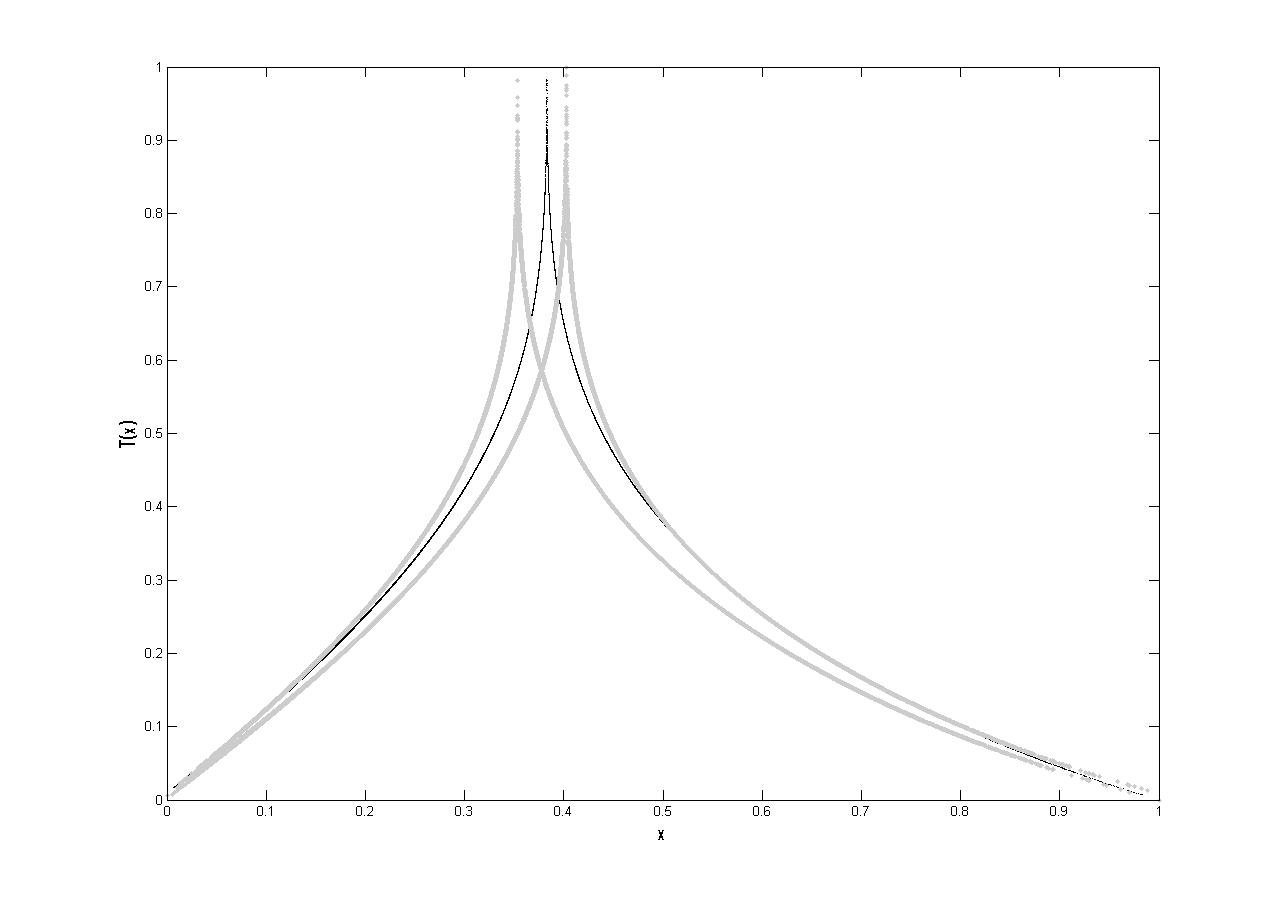
Figure 2: experimental plots of the unperturbed map $\tilde{T}_{0}$ (in black) and of its perturbations (in grey).

In the case $\mathcal{M}:=\mathcal{M}^{\prime\prime},\Gamma_{0}=\left\{c_{0}\right\}.$ Hence, we identify $I$ with $\left[-1,1\right]$ and, again with abuse of notation, we denote by $\bar{T}_{\eta}:\left[-1,1\right]\circlearrowleft$ the map

$$\left[-1,1\right]\ni u\longmapsto\bar{T}_{\eta}\left(u\right) :=\mathbf{1}_{\left[-1,-u_{0,\eta}^{2}\right]}\left(u\right)\tilde{T}_{\eta,2}\left(-u\right)-\mathbf{1}_{\left[-u_{0,\eta}^{2},0\right]}\left(u\right)\tilde{T}_{\eta,2}\left(-u\right)+$$ (225)

$$+\mathbf{1}_{\left[0,u_{0,\eta}^{1}\right]}\left(u\right)\tilde{T}_{\eta,1}\left(u\right)-\mathbf{1}_{\left[u_{0,\eta}^{1},1\right]}\left(u\right)\tilde{T}_{\eta,2}\left(u\right)\in\left[-1,1\right]\ ,$$

where, for $i=1,2,\tilde{T}_{\eta,i}:\left[0,1\right]\circlearrowleft$ is a transitive, continuous Lorenz-like cusp map of the interval of the type studied in [GMPV], with two branches and a point $u_{0,\eta}^{i}\in\left[0,1\right]$ such that $\tilde{T}_{\eta,i}\left(\left(u_{0,\eta}^{i}\right)^{-}\right)=\tilde{T}_{\eta,i}\left(\left(u_{0,\eta}^{i}\right)^{+}\right)=1.$

In fact, in [PM], the paper that inspired our previous work [GMPV], the authors showed that the invariant measure for $\bar{T}_{\eta}$ can be deduced directly from those of the $\tilde{T}_{\eta,i}$’s, whose local behaviour is therefore the following (compare formulas (52)-(55) in [GMPV] and Figure 2):

$$\tilde{T}_{\eta,i}\left(u\right)=\left\{\begin{array}[c]{ll}a_{\eta,i}u+b_{\eta,i}u^{1+c_{\eta,i}}+o(u^{1+c_{\eta,i}})\ ;\ a_{\eta,i}\ ,\ c_{\eta,i}>1,b_{\eta,i}>0&u\rightarrow 0^{+}\\ 1-A_{\eta,i}(u_{0,\eta}-u)^{B_{\eta,i}}+o((u_{0,\eta}-u)^{B_{\eta,i}})\ ;\ A_{\eta,i}>0,B_{\eta,i}\in\left(0,1\right)&u\rightarrow\left(u_{0,\eta}^{i}\right)^{-}\\ 1-A_{\eta,i}^{\prime}(u-u_{0,\eta})^{B_{\eta,i}^{\prime}}+o((u-u_{0,\eta})^{B_{\eta,i}^{\prime}})\ ;\ A_{\eta,i}^{\prime}>0,B_{\eta,i}^{\prime}\in\left(0,1\right)&u\rightarrow\left(u_{0,\eta}^{i}\right)^{+}\\ a_{\eta,i}^{\prime}\left(1-u\right)+b_{\eta,i}^{\prime}\left(1-u\right)^{1+c_{\eta,i}^{\prime}}+o(\left(1-u\right)^{1+c_{\eta,i}^{\prime}})\ ;\ a_{\eta,i}^{\prime}\in\left(0,1\right),b_{\eta,i}^{\prime}>0,c_{\eta,i}^{\prime}>1&u\rightarrow 1^{-}\end{array}\right.\ .$$ (226)

We remark that to prove the stochastic stability of the invariant measure for the evolution defined by the unperturbed map $T_{0}$ we needed supplementary assumptions on $T_{0};$ see Section 8.4.

In particular, in the case $\mathcal{M}:=\mathcal{M}^{\prime\prime},$ by construction the stochastic stability of $T_{0}$ will follow from that of $\tilde{T}_{0}.$

13 Existence of invariant measures for the Lorenz-type cusp map

In our previous paper [GMPV] the one-dimensional Lorenz-cusp type map $T$ ($\tilde{T}$ in the present paper) had a branch with first derivative less than one on a open set but still bounded from below by a positive number. We were unable to show that the derivative became globally larger that one for a suitable power of the map and therefore we proceeded differently to prove the statistical stability of the unperturbed invariant measure; namely we induced and we showed that on a (lot of) induced set(s), the derivative of the first return map was uniformly larger than one.

Anyway, the existence of an invariant measure for $T$ follows combining Theorem 2 in [Pi] and the results in section 4.2 of [Bu] since one can check by direct computation that the map

$$I\ni u\longmapsto\overline{T}\left(u\right):=W\circ T\circ W^{-1}\left(u\right)\in I\ ,$$ (227)

where $W$ is the distribution function associated to the probability measure on $\left(\left[0,1\right],\mathcal{B}\left(\left[0,1\right]\right)\right)$ with density

$$\left[0,1\right]\ni x\longmapsto W^{\prime}\left(x\right):=N_{\bar{\gamma},\bar{\beta}}e^{-\bar{\gamma}x}x^{\bar{\beta}}\left(1-x\right)^{\bar{\beta}}$$ (228)

(see formulas (83) and (84) in [GMPV]) for suitably chosen parameters $\bar{\gamma},\bar{\beta}>0$ is such that $\inf\left|\overline{T}^{\prime}\right|>1.$

In particular, by (226), for any $\eta\in spt\lambda_{\varepsilon},$ setting $B_{\eta}^{\ast}:=B_{\eta}\vee B_{\eta}^{\prime}$ and choosing $0<\bar{\beta}<\inf_{\eta\in spt\lambda_{\varepsilon}}\frac{1}{B_{\eta}^{\ast}}-1,\bar{\gamma}>\sup_{\eta\in spt\lambda_{\varepsilon}}\frac{\bar{\beta}+1}{1-x_{0,\eta}}\log\frac{1}{a_{\eta}^{\prime}},$ for any $\eta\in spt\lambda_{\varepsilon},$ we get $\inf_{\eta\in spt\lambda_{\varepsilon}}\inf\left|\overline{T}_{\eta}^{\prime}\right|>1.$ Hölder continuity of $\frac{1}{\overline{T}_{\eta}^{\prime}}$ follows from (229).

14 Statistical stability for Lorenz-like cusp maps

We take the chance to rectify an incorrect statement we made in [GMPV] about the regularity properties of the one-dimensional map $T.$

Therefore, in this section, we will use the same notation we used in [GMPV].

In that paper we state that the map $T$ was $C^{1+\iota},$ for some $\iota\in\left(0,1\right),$ on the union of the two sets $(0,x_{0}),(x_{0},1),$ where the map was $1$ to $1.$ This is incorrect. What is true is that $T^{-1}$ is $C^{1+\iota},$ for some $\iota\in\left(0,1\right),$ on each open interval $(0,x_{0}),(x_{0},1).$ Indeed, by the result in [AM], the stable foliation for the classical Lorenz flow is $C^{1+\alpha}$ for some $\alpha\in\left(0.278,1\right),$ which means, by (54) and (55) in [GMPV], that, for any $x\in(0,x_{0}),T^{{}^{\prime}}\left(x\right)=\left|x_{0}-x\right|^{1-B^{\prime}}\left[1+G_{1}\left(x\right)\right]$ with $G_{1}\in C^{\alpha B^{\prime}}(0,x_{0})$ and, for any $x\in(x_{0},1),T^{\prime}\left(x\right)=\left|x-x_{0}\right|^{1-B}\left[1+G_{2}\left(x\right)\right]$ with $G_{2}\in C^{\alpha B}(x_{0},1).$ In particular this implies that for any couple of points $x,y$ belonging either to $(0,x_{0})$ or to $(x_{0},1)$

$$|T^{\prime}(x)-T^{\prime}(y)|\leq C_{h}\left|T^{\prime}(x)\right|\left|T^{\prime}(y)\right|\left|x-y\right|^{\iota}\ ,$$ (229)

where $\iota\in(0,1-B^{\ast}],$ with $B^{\ast}:=B\vee B^{\prime},$ and the constant $C_{h}$ is independent of the location of $x$ and $y.$

We now detail the modifications that these corrections induce on some of the proofs of the results given in [GMPV], all the statements of our results remaining unchanged.

Distortion

The proof of the boundedness of the distortion was sketched in the footnote (1) of [GMPV] by using arguments given in [CHMV]. In particular, in the initial formula (5) in [CHMV] we need now to replace the term $\left|\frac{D^{2}T(\xi)}{DT(\xi)}\right||T^{q}\left(x\right)-T^{q}\left(y\right)|,$ where $\xi$ is a point between $T^{q}\left(x\right)$ and $T^{q}\left(y\right),$ with $\frac{1}{|DT(\xi)|}C_{h}|DT(T^{q}\left(x\right))||DT(T^{q}\left(y\right))||T^{q}\left(x\right)-T^{q}\left(y\right)|^{\iota}$ which is smaller than $C_{h}\left(|DT(T^{q}\left(x\right))|\vee|DT(T^{q}\left(y\right))|\right)|T^{q}\left(x\right)-T^{q}\left(y\right)|^{\iota}$ by monotonicity of $\left|DT\right|.$ The key estimate (11) in [CHMV] will reduce in our case to the bound of the quantity $\sup_{\xi\in[b_{i+1},b_{i}]}|DT\left(\xi\right)||b_{i}-b_{i+1}|.$ By using for $DT$ the expressions given in the formulas (54) and (55) of [GMPV], and for the $b_{i}$ the scaling given in formula (75) of the same paper, we immediately get that the above quantity is of order $\frac{1}{(\alpha^{\prime})^{i}},$ which is enough to pursue the argument about the estimate of the distortion presented in [CHMV].

Perturbation

In order to prove the statistical stability of the invariant measure $\mu_{T}$ for the evolution given by the map $T,$ the perturbed map $T_{\epsilon}$ must satisfy at least the same regularity properties required for $T.$ Therefore, in [GMPV] Section 3.2:

• Assumption A should be replaced by the assumption that there exists $\iota_{\epsilon}\in\left(0,1\right)$ such that $T\upharpoonleft_{(0,x_{\epsilon,0})},T\upharpoonleft_{(x_{\epsilon,0},1)}$ are $C^{1+\iota_{\epsilon}}$ rather than assuming the stronger requirement that $T_{\epsilon}$ is $C^{1+\iota_{\epsilon}}$ on $(0,x_{\epsilon,0})\cup(x_{\epsilon,0},1);$

• Assumption C should be replaced by the requirement that the multiplicative Hölder constant $C_{h}^{\epsilon}$ of $D\left(T_{\epsilon}^{-1}\right)$ will converge to $C_{h}$ when $\epsilon\rightarrow 0.$

We have then to modify the bounds (92), (99) and (114) in [GMPV] which are all of the form $|DT_{\epsilon}(a)-DT_{\epsilon}(a_{\epsilon})|,$ with $a$ $\epsilon$-close to $a_{\epsilon}.$ We have $|DT_{\epsilon}(a)-DT_{\epsilon}(a_{\epsilon})|\leq C_{h}^{\epsilon}|DT_{\epsilon}(a)||DT_{\epsilon}(a_{\epsilon})||a-a_{\epsilon}|.$ By the continuity and the monotonicity of $DT_{\epsilon}$ we can replace $a_{\epsilon}$ in $|DT_{\epsilon}(a_{\epsilon})|$ with $a$ or with another given point between $a$ and $x_{0};$ finally we use the limit (88) in Assumption B to conclude.

15 Proof of Proposition 2

Proof. The invariance of $\mu_{\overline{\mathbf{R}}}$ under $\overline{\mathbf{R}}$ follows by (68), since

$$\mu_{\overline{\mathbf{R}}}\left(\psi\circ\overline{\mathbf{R}}\right):=\lim_{n\rightarrow\infty}\int\mu_{\mathbf{T}}\left(du,d\omega\right)\inf_{x\in q^{-1}\left(u\right)}\psi\circ\overline{\mathbf{R}}^{n+1}\left(x,\omega\right)=\mu_{\overline{\mathbf{R}}}\left(\psi\right)\ .$$ (230)

Hence, since

$$\lim_{n\rightarrow\infty}\int\mu_{\mathbf{T}}\left(du,d\omega\right)\inf_{x\in q^{-1}\left(u\right)}\psi\circ\overline{\mathbf{R}}^{n}\left(x,\omega\right) \leq\lim_{n\rightarrow\infty}\int\mu_{\mathbf{T}}\left(du,d\omega\right)\left(\left(\mathbf{1}_{q^{-1}\left(u\right)}\circ p\right)\psi\right)\circ\overline{\mathbf{R}}^{n}\left(x,\omega\right)$$ (231)

$$\leq\lim_{n\rightarrow\infty}\int\mu_{\mathbf{T}}\left(du,d\omega\right)\sup_{x\in q^{-1}\left(u\right)}\psi\circ\overline{\mathbf{R}}^{n}\left(x,\omega\right)\ ,$$

it is enough to prove that

$$\lim_{n\rightarrow\infty}\int\mu_{\mathbf{T}}\left(du,d\omega\right)\inf_{x\in q^{-1}\left(u\right)}\psi\circ\overline{\mathbf{R}}^{n}\left(x,\omega\right)=\lim_{n\rightarrow\infty}\int\mu_{\mathbf{T}}\left(du,d\omega\right)\sup_{x\in q^{-1}\left(u\right)}\psi\circ\overline{\mathbf{R}}^{n}\left(x,\omega\right)\ .$$ (232)

By (48), (32) and the definition of $\bar{R}_{\pi\left(\omega\right)},\forall\omega\in\Omega,$

$$\overline{\mathbf{R}}\left(Q^{-1}\left(u,\omega\right)\right)\subset Q^{-1}\left(\mathbf{T}\left(u,\omega\right)\right)\ .$$ (233)

Therefore,

$$\sup_{x\in q^{-1}\left(u\right)}\psi\circ\overline{\mathbf{R}}^{n+k}\left(x,\omega\right) =\sup_{\left(x,\omega^{\prime}\right)\in Q^{-1}\left(u,\omega\right)}\psi\circ\overline{\mathbf{R}}^{n+k}\left(x,\omega^{\prime}\right)$$ (234)

$$\leq\sup_{\left(x,\omega^{\prime}\right)\in Q^{-1}\left(\mathbf{T}^{k}\left(u,\omega\right)\right)}\psi\circ\overline{\mathbf{R}}^{n}\left(x,\omega^{\prime}\right)$$

$$=\sup_{\left(x,\omega^{\prime}\right)\in\left\{\left(y,\omega^{\prime\prime}\right)\in\mathcal{M}\times\Omega\ :\ Q\left(y,\omega^{\prime\prime}\right)=\mathbf{T}^{k}\left(u,\omega\right)\right\}}\psi\circ\overline{\mathbf{R}}^{n}\left(x,\omega^{\prime}\right)$$

and

$$\inf_{x\in q^{-1}\left(u\right)}\psi\circ\overline{\mathbf{R}}^{n+k}\left(x,\omega\right) =\inf_{\left(x,\mathbf{\omega}^{\prime}\right)\in Q^{-1}\left(u,\omega\right)}\psi\circ\overline{\mathbf{R}}^{n+k}\left(x,\omega^{\prime}\right)$$ (235)

$$\geq\inf_{\left(x,\omega^{\prime}\right)\in Q^{-1}\left(\mathbf{T}^{k}\left(u,\omega\right)\right)}\psi\circ\overline{\mathbf{R}}^{n}\left(x,\omega^{\prime}\right)$$

$$=\inf_{\left(x,\omega^{\prime}\right)\in\left\{\left(y,\omega^{\prime\prime}\right)\in\mathcal{M}\times\Omega\ :\ Q\left(y,\omega^{\prime\prime}\right)=\mathbf{T}^{k}\left(u,\omega\right)\right\}}\psi\circ\overline{\mathbf{R}}^{n}\left(x,\omega^{\prime}\right)\ .$$

Hence, by the invariance of $\mu_{\mathbf{T}}$ under $\mathbf{T},$

$$\int\mu_{\mathbf{T}}\left(du,d\omega\right)\sup_{x\in q^{-1}\left(u\right)}\psi\circ\overline{\mathbf{R}}^{n+k}\left(x,\omega\right)\leq\int\mu_{\mathbf{T}}\left(du,d\omega\right)\sup_{\left(x,\omega^{\prime}\right)\in\left\{\left(y,\omega^{\prime\prime}\right)\in\mathcal{M}\times\Omega\ :\ Q\left(y,\omega^{\prime\prime}\right)=\mathbf{T}^{k}\left(u,\omega\right)\right\}}\psi\circ\overline{\mathbf{R}}^{n}\left(x,\omega^{\prime}\right)$$ (236)

$$=\int\left(\mathbf{T}_{\#}^{k}\mu_{\mathbf{T}}\right)\left(du,d\omega\right)\sup_{\left(x,\omega^{\prime}\right)\in\left\{\left(y,\omega^{\prime\prime}\right)\in\mathcal{M}\times\Omega\ :\ Q\left(y,\omega^{\prime\prime}\right)=\left(u,\omega\right)\right\}}\psi\circ\overline{\mathbf{R}}^{n}\left(x,\omega^{\prime}\right)$$

$$=\int\mu_{\mathbf{T}}\left(du,d\omega\right)\sup_{\left(x,\omega^{\prime}\right)\in Q^{-1}\left(u,\omega\right)}\psi\circ\overline{\mathbf{R}}^{n}\left(x,\omega^{\prime}\right)$$

$$=\int\mu_{\mathbf{T}}\left(du,d\omega\right)\sup_{x\in q^{-1}\left(u\right)}\psi\circ\overline{\mathbf{R}}^{n}\left(x,\omega\right)$$

so that the sequence $\left\{\int\mu_{\mathbf{T}}\left(du,d\omega\right)\sup_{x\in q^{-1}\left(u\right)}\psi\circ\overline{\mathbf{R}}^{n}\left(x,\omega\right)\right\}_{n\geq 1}$ is decreasing. On the other hand,

$$\int\mu_{\mathbf{T}}\left(du,d\omega\right)\inf_{x\in q^{-1}\left(u\right)}\psi\circ\overline{\mathbf{R}}^{n+k}\left(x,\omega\right)\geq\int\mu_{\mathbf{T}}\left(du,d\omega\right)\inf_{\left(x,\omega^{\prime}\right)\in\left\{\left(y,\omega^{\prime\prime}\right)\in\mathcal{M}\times\Omega\ :\ Q\left(y,\omega^{\prime\prime}\right)=\mathbf{T}^{k}\left(u,\omega\right)\right\}}\psi\circ\overline{\mathbf{R}}^{n}\left(x,\omega^{\prime}\right)$$ (237)

$$=\int\left(\mathbf{T}_{\#}^{k}\mu_{\mathbf{T}}\right)\left(du,d\omega\right)\inf_{\left(x,\omega^{\prime}\right)\in\left\{\left(y,\omega^{\prime\prime}\right)\in\mathcal{M}\times\Omega\ :\ Q\left(y,\omega^{\prime\prime}\right)=\left(u,\omega\right)\right\}}\psi\circ\overline{\mathbf{R}}^{n}\left(x,\omega^{\prime}\right)$$

$$=\int\mu_{\mathbf{T}}\left(du,d\omega\right)\inf_{\left(x,\omega^{\prime}\right)\in Q^{-1}\left(u,\omega\right)}\psi\circ\overline{\mathbf{R}}^{n}\left(x,\omega^{\prime}\right)$$

so that $\left\{\int\mu_{\mathbf{T}}\left(du,d\omega\right)\inf_{x\in q^{-1}\left(u\right)}\psi\circ\overline{\mathbf{R}}^{n}\left(x,\omega\right)\right\}_{n\geq 1}$ is increasing. Since $\forall\omega\in\Omega,\psi\left(\cdot,\omega\right)\in C_{b}\left(\mathcal{M}\right)$ and $\forall u\in I,q^{-1}\left(u\right)\subset\mathcal{M}$ is compact, by (233), $\forall\varepsilon^{\prime}>0,\exists\delta_{\varepsilon^{\prime}}>0,n_{\varepsilon^{\prime}}>0$ such that $\forall n\geq n_{\varepsilon^{\prime}},\omega\in\Omega,u\in I,\operatorname*{diam}p\left(\overline{\mathbf{R}}^{n}\left(Q^{-1}\left(u,\omega\right)\right)\right)<\delta_{\varepsilon^{\prime}}$ and $\forall\left(x,\omega^{\prime}\right),\left(y,\omega^{\prime}\right)\in\overline{\mathbf{R}}^{n}\left(Q^{-1}\left(u,\omega\right)\right),$$\left|\psi\left(x,\omega^{\prime}\right)-\psi\left(y,\omega^{\prime}\right)\right|<\varepsilon^{\prime},$ therefore

$$\left|\int\mu_{\mathbf{T}}\left(du,d\omega\right)\sup_{x\in q^{-1}\left(u\right)}\psi\circ\overline{\mathbf{R}}^{n}\left(x,\omega\right)-\int\mu_{\mathbf{T}}\left(du,d\omega\right)\inf_{x\in q^{-1}\left(u\right)}\psi\circ\overline{\mathbf{R}}^{n}\left(x,\omega\right)\right|$$ (238)

$$\leq\int\mu_{\mathbf{T}}\left(du,d\omega\right)\left|\sup_{\left(x,\omega^{\prime}\right)\in Q^{-1}\left(u,\omega\right)}\psi\circ\overline{\mathbf{R}}^{n}\left(x,\omega^{\prime}\right)-\inf_{\left(x,\omega^{\prime}\right)\in Q^{-1}\left(u,\omega\right)}\psi\circ\overline{\mathbf{R}}^{n}\left(x,\omega^{\prime}\right)\right|\leq\varepsilon^{\prime}\ ,$$

that is (232) holds.

Thus, the map

$$L_{\mathbb{P}}^{1}\left(\Omega,C_{b}\left(\mathcal{M}\right)\right)\ni\psi\longmapsto\hat{\mu}\left(\psi\right):=\lim_{n\rightarrow\infty}\int\mu_{\mathbf{T}}\left(du,d\omega\right)\left(\left(\mathbf{1}_{q^{-1}\left(u\right)}\circ p\right)\psi\right)\circ\overline{\mathbf{R}}^{n}\left(x,\omega\right)\in\mathbb{R}$$ (239)

is a non negative linear functional such that $\hat{\mu}\left(1\right)=1$ and, by (232),

$$\hat{\mu}\left(\psi\right)=\lim_{n\rightarrow\infty}\int\mu_{\mathbf{T}}\left(du,d\omega\right)\inf_{x\in q^{-1}\left(u\right)}\psi\circ\overline{\mathbf{R}}^{n}\left(x,\omega\right)\ .$$ (240)

Moreover, $\Omega$ is compact under the product topology, then the space of quasi-local continuous functions $C_{\infty}\left(\Omega,C_{b}\left(\mathcal{M}\right)\right)$ is dense in $L_{\mathbb{P}}^{1}\left(\Omega,C_{b}\left(\mathcal{M}\right)\right),$ therefore, by the Riesz-Markov-Kakutani theorem there exists a unique Radon measure $\mu_{\overline{\mathbf{R}}}$ on $\left(\mathcal{M}\times\Omega,\mathcal{B}\left(\mathcal{M}\right)\otimes\mathcal{F}\right)$ such that $\mu_{\overline{\mathbf{R}}}=\hat{\mu}\upharpoonleft_{C_{K}\left(\Omega,C_{b}\left(\mathcal{M}\right)\right)}.$

The injectivity of the correspondence $\mu_{\mathbf{T}}\longmapsto\mu_{\overline{\mathbf{R}}}$ follows from the fact that, $\forall\varphi\in L_{\mathbb{P}}^{1}\left(\Omega,C_{b}\left(I\right)\right),\varphi\circ Q\in L_{\mathbb{P}}^{1}\left(\Omega,C_{b}\left(\mathcal{M}\right)\right)$ and

$$\int\mu_{\mathbf{T}}\left(du,d\omega\right)\inf_{x\in q^{-1}\left(u\right)}\varphi\circ Q\circ\overline{\mathbf{R}}^{n}\left(x,\omega\right)=\int\mu_{\mathbf{T}}\left(du,d\omega\right)\inf_{x\in q^{-1}\left(u\right)}\varphi\circ\mathbf{T}^{n}\circ Q\left(x,\omega\right)$$ (241)

$$=\int\mu_{\mathbf{T}}\left(du,d\omega\right)\inf_{x\in q^{-1}\left(u\right)}\varphi\circ\mathbf{T}^{n}\left(q\left(x\right),\omega\right)=\mu_{\mathbf{T}}\left(\varphi\circ\mathbf{T}^{n}\right)=\mu_{\mathbf{T}}\left(\varphi\right)\ .$$

Therefore, if there exist $\mu_{\mathbf{T}}^{\prime}$ invariant under $\mathbf{T}$ such that

$$\mu_{\overline{\mathbf{R}}}\left(\psi\right):=\lim_{n\rightarrow\infty}\int\mu_{\mathbf{T}}^{\prime}\left(du,d\omega\right)\inf_{x\in q^{-1}\left(u\right)}\psi\circ\overline{\mathbf{R}}^{n}\left(x,\omega\right)\ ,$$ (242)

then $\mu_{\mathbf{T}}^{\prime}\left(\varphi\right)=\mu_{\mathbf{T}}\left(\varphi\right),$ hence $\mu_{\mathbf{T}}^{\prime}=\mu_{\mathbf{T}}.$

The proof of the ergodicity of $\mu_{\overline{\mathbf{R}}}$ under the hypotesis of the ergodicity of $\mu_{\mathbf{T}}$ is identical to that of Corollary 7.25 in Section 7.3.4 of [AP].

References

• [Al] Alsmeyer G. The Markov Renewal Theorem and Related Results Markov Proc. Rel. Fields 3, 103–127 (1997).
• [Ar] Arnold L. Random Dynamical Systems Springer (2003).
• [As] Asmussen S., Applied Probability and Queues, II edition Springer (2003).
• [ABS] V.S. Afraimovic, V.V. Bykov, Sili’nikov L.P. The origin and structure of the Lorenz attractor Dokl. Akad. Nauk SSSR 234, no. 2, 336–339 (1977).
• [AM] Araújo V., Melbourne I. Existence and smoothness of the stable foliation for sectional hyperbolic attractors Bull. London Math. Soc. 49 351–367 (2017).
• [AMV] Araújo V., Melbourne I., Varandas P. Rapid Mixing for the Lorenz Attractor and Statistical Limit Laws for Their Time-1 Maps Commun. Math. Phys. 340, 901–938 (2015).
• [AP] Araújo V., Pacifico M. J. Three-dimesional flows Springer (2010).
• [APPV] Araújo V., Pacifico M. J., Pujals E. R., Viana, M. Singular-hyperbolic attractors are chaotic Trans. Amer. Math. Soc. 361 n. 5, 2431–2484 (2008).
• [AS] Alves, J. F.,Soufi, M. Statistical stability of geometric Lorenz attractors Fundamenta Mathematicae 224, 219–231 (2014).
• [BHV] Bahsoun W., Hu H.-Y. Vaienti S. Pseudo-orbits, stationary measures and metastability Dyn. Syst. 29 n. 3 322–336 (2014).
• [BR] Bahsoun W., Ruziboev M. On the stability of statistical properties for the Lorenz attractors with $C^{1+\alpha}$ stable foliation Ergodic Theor. and Dyn. Sys. 39, n.12, 3169–3184 (2019).
• [Bu] Butterley O. Area expanding $C^{1+\alpha}$ Suspension Semiflows Commun. Math. Phys. 325 n.2, 803–820 (2014).
• [CHMV] Cristadoro, G-P., Haydn, N., Marie, Ph., Vaienti, S. Statistical properties of intermittent maps with unbounded derivative Nonlinearity 23, 1071–1095 (2010).
• [CMP] S. Corti, F. Molteni, T. N. Palmer Signature of recent climate change in frequencies of natural atmospheric circulation regimes Letters to Nature 398, 799–802 (1999).
• [CSG] Chekroun, M. D., Simonnet E., Ghil M. Stochastic climate dynamics: random attractors and time-independent invariant measures Phisica D 240 n.21, 1685–1700 (2011).
• [Da] M. H. A. Davis Markov Models and Optimization Springer (1993).
• [GHL] D. Guibourg, L. Hervé, J. Ledoux Quasi-compactness of Markov kernels on weighted-supremum spaces and geometrical ergodicity arXiv:1110.3240v5
• [GL] Galatolo S., Lucena R. Spectral gap and quantitative statistical stability for systems with contracting fibers and Lorenz-like maps Discrete Contin. Dyn. Syst. 40, n.3, 1309–1360 (2020).
• [GMPV] Gianfelice M., Maimone F., Pelino V., Vaienti S. On the recurrence and robust properties of the Lorenz’63 model Commun. Math. Phys. 313, 745–779 (2012).
• [GW] Gukenheimer J., Williams R.F. Structural stability of Lorenz attractors Inst. Hautes Etudes Sci. Publ. Math. 50, 59–72 (1979).
• [HM] Holland M., Melbourne I. Central limit theorems and invariance principles for Lorenz attractors J. London Math. Soc. 2, 76, 345364 (2007).
• [HS] Hirsch M. W., Smale S. Differential Equations, Dynamical Systems, and Linear Algebra Academic press (1978).
• [Ke] Keller H. Attractors and bifurcations of the stochastic Lorenz system Report 389, Institut für Dynamische Systeme, Universität Bremen (1996).
• [Ki] Kifer Y. Random Perturbations of Dynamical Systems Birkhäuser (1988).
• [KL] Keller G., Liverani C. Stability of the spectrum for transfer operators Ann. Scuola Norm. Sup. Pisa Cl. Sci. (4) 28 n. 1, 141–152 (1999).
• [KS] Korolyuk V., Swishchuk A. Semi-Markov Random Evolutions Springer (1995).
• [Lo] Lorenz E. N. Deterministic Nonperiodic Flow J. Atmos. Sci., vol. 20, 130–141 (1963).
• [Me] Metzger R. J. Stochastic Stability for Contracting Lorenz Maps and Flows Comm. Math. Phys. 212, 277–296 (2000).
• [MT] Meyn S. Tweedie R. L. Markov Chains and Stochastic Stability, Second Edition Cambridge University Press (2009).
• [NVKDF] Nevo G., Vercauteren N., Kaiser A., Dubrulle B., Faranda D. A statistical-mechanical approach to study the hydrodynamic stability of stably stratified atmospheric boundary layer Phys. Rev. Fluids 2, 084603 (2017).
• [Pa] Palmer T. N. A Nonlinear Dynamical Perspective on Climate Prediction Journal of Climate 12 n.2, 575–591 (1999).
• [Pi] Pianigiani G. Existence of invariant measures for piecewise continuous transformations Annales Polonici Mathematici XL, 3945 (1981).
• [PM] Pelino V., Maimone F. Energetics, skeletal dynamics, and long term predictions on Kolmogorov-Lorenz systems Physical Review E, 76, 046214 (2007).
• [PP] Pasini A., Pelino V. A unified view of Kolmogorov and Lorenz systems Phys. Lett. A 275, 435–445 (2000).
• [Sa] Saussol, B. Absolutely continuous invariant measures for multidimensional expanding maps Israel Journal of Mathematics 116 223–248 (2000).
• [Sc] Schmallfuß, B. The random attractor of the stochastic Lorenz system Z. angew. Math. Phys. 48 951–975 (1997).
• [Su] Sura P. A general perspective of extreme events in weather and climate Atmospheric Research 101 1–21 (2011).
• [Tu] W. Tucker A rigorous ODE solver and Smale’s 14th problem Foundations of Computational Mathematics, 2:1 53–117 (2002).
• [Vi] Viana M. Stochastic Dynamics of Deterministic Systems IMPA notes (1997).