Galactic Archeology with the AEGIS Survey: The Evolution of Carbon and Iron in the Galactic Halo

Abstract

Understanding the evolution of carbon and iron in the Milky Way’s halo is of importance because these two elements play crucial roles constraining star formation, Galactic assembly, and chemical evolution in the early Universe. Here, we explore the spatial distributions of carbonicity, [C/Fe], and metallicity, [Fe/H], of the halo system based on medium-resolution ($R\sim$ 1,300) spectroscopy of $\sim$58,000 stars in the Southern Hemisphere from the AAOmega Evolution of Galactic Structure (AEGIS) survey. The AEGIS carbonicity map exhibits a positive gradient with distance, as similarly found for the Sloan Digital Sky Survey (SDSS) carbonicity map of Lee et al. The metallicity map confirms that [Fe/H] decreases with distance, from the inner halo to the outer halo. We also explore the formation and chemical-evolution history of the halo by considering the populations of carbon-enhanced metal-poor (CEMP) stars present in the AEGIS sample. The cumulative and differential frequencies of CEMP-no stars (as classified by their characteristically lower levels of absolute carbon abundance, $A$(C) $\leq$ 7.1 for sub-giants and giants) increases with decreasing metallicity, and is substantially higher than previous determinations for CEMP stars as a whole. In contrast, that of CEMP-$s$ stars (with higher $A$(C)), remains almost flat, at a value $\sim$10%, in the range $-\,4.0\lesssim$ [Fe/H] $\lesssim-$2.0. The distinctly different behaviors of the CEMP-no and CEMP-$s$ stars relieve the tension with population-synthesis models assuming a binary mass-transfer origin, which previously struggled to account for the higher reported frequencies of CEMP stars, taken as a whole, at low metallicity.

1 Introduction

The present chemical composition of stars in the Milky Way (with the exception of hydrogen and helium) comprises various nucleosynthetic products, forged in previous generations of stars. First-generation stars, which are expected to be massive stars formed from primordial gas, synthesized metals up to the iron peak via stages of stellar nucleosynthesis in their interiors, and (possibly) elements such as Sr or Ba via a weak slow neutron-capture process (weak $s$-process, e.g., Maeder & Meynet, 2015; Frischknecht et al., 2016). Iron-peak elements are also created via explosive nucleosynthesis (e.g., Nomoto et al., 2013, and references therein) by supernovae associated with massive stars. Beyond the iron peak, roughly half of the heavy elements are produced in low- to intermediate-mass stars by the main $s$-process during the asymptotic giant-branch (AGB) phase (e.g., Frost & Lattanzio, 1996; Lugaro et al., 2003; Herwig, 2005; Karakas & Lattanzio, 2014). The so-called “intermediate” neutron-capture process or $i$-process (possibly operating in high-mass AGB stars) may also play a role (Cowan & Rose, 1977; Dardelet et al., 2015; Hampel et al., 2016). Other heavy metals beyond the Fe-peak are created by the main rapid neutron-capture process ($r$-process), likely associated with neutron star mergers (e.g., Lattimer & Schramm, 1974; Meyer, 1989; Rosswog et al., 2014; Abbott et al., 2017; Drout et al., 2017; Shappee et al., 2017, and references therein), but could also involve so-called magneto-rotational instability or ”jet” supernovae (Cameron, 2003; Fujimoto et al., 2008; Winteler et al., 2012), or neutrino-driven winds in core-collapse supernovae (Arcones & Thielemann, 2013, and references therein). In addition, there is another process, referred to as the weak or limited $r$-process (Travaglio et al., 2004; Wanajo & Ishimaru, 2006; Frebel, 2018), whose astrophysical site(s) are not yet clear, but it is thought to be associated with supernovae origins (Izutani et al., 2009; Nomoto et al., 2013). This process can explain the moderate enhancements of light neutron-capture elements such as Sr, Y, and Zr relative to elements heavier than Ba, a signature that appears distinct from other neutron-capture processes (see, e.g., Honda et al. 2007).

All of the elements play potentially important roles in our understanding of Galactic chemical evolution (GCE), since the production history of each element can follow different nucleosynthesis pathways (exploring different astrophysical processes, sites, timescales, and/or stellar-progenitor masses). However, in this work we focus on two fundamental elements, carbon and iron. These two elements are of special significance, because they serve as tracers of the stellar populations that were present from the earliest times in the chemical evolution of the Galaxy.

1.1 Carbon as a Tracer of Stellar Populations and GCE

The observed abundances of most of the light and heavy elements in stars scale with the overall metallicity. However, as pointed out by Beers et al. (1992), carbon (and a number of other light elements, including N and O) is a notable exception. An increasing fraction of low-metallicity stars exhibit carbon enhancement with declining metallicity, approaching 100% at the lowest iron abundances (Placco et al., 2014).

In the very early universe (likely within the first few hundred million years following the Big Bang), carbon is thought to be ejected primarily by so-called “faint” supernovae (e.g., Umeda & Nomoto, 2003, 2005; Nomoto et al., 2013; Tominaga et al., 2014) of massive first-generation stars, by the stellar winds from massive, rapidly rotating spinstars (e.g., Meynet et al., 2006, 2010; Chiappini, 2013), and by core-collapse supernovae from massive stars. Pollution of the surrounding pristine interstellar medium (inside and outside the natal clouds of the first stars) by carbon provided pathways for efficient gas cooling and fragmentation, enabling the formation of low- and intermediate-mass stars (e.g., Bromm & Loeb, 2003; Schneider et al., 2003, 2012; Omukai et al., 2005; Frebel et al., 2007).

The progeny of the very first stars are expected to exhibit extremely low iron (and other heavy-element) content and greatly enhanced carbon. This first-star nucleosynthetic signature is matched by the sub-class of carbon-enhanced metal-poor (CEMP; Beers & Christlieb 2005; Aoki et al. 2007) stars known as CEMP-no stars (e.g., Christlieb et al., 2004; Meynet et al., 2006; Frebel et al., 2008; Nomoto et al., 2013; Keller et al., 2014; Bonifacio et al., 2015; Yoon et al., 2016; Placco et al., 2016b; Chiaki et al., 2017; Choplin et al., 2017, and references therein).

Beginning roughly a Gyr later, the dominant carbon-production pathway is replaced by AGB nucleosynthesis in intermediate- and lower-mass stars. This nucleosynthetic signature (an enhancement of both carbon and $s$-process elements) can be preserved on the surfaces of long-lived low-mass binary companions following a mass-transfer event from the erstwhile AGB stars (e.g., Lugaro et al., 2012; Placco et al., 2013). The CEMP-$s$ (and possibly CEMP-$i$, Hampel et al. 2016) stars found at extremely and very low metallicity (but so far not at the lowest metallicity, [Fe/H]$<-$4.0) are the living records of this era.

Nature’s dual carbon-production pathways in cosmic time were first recognized as high and low bands of absolute carbon abundance, $A$(C), in the $A$(C) vs. [Fe/H] space (Spite et al., 2013), based on a sample of $\sim 50$ “un-mixed” turnoff stars. This behavior was supported by Bonifacio et al. (2015), based on $\sim$70 CEMP stars, including a number of mildly evolved sub-giants. The full richness of the behavior of CEMP stars in this space was revealed in the Figure 1 of Yoon et al. (2016) – the Yoon-Beers diagram – based on a large literature sample of $\sim$300 CEMP stars with available high-resolution spectroscopy. Not only did this diagram identify two primary peaks in the marginal plot of $A$(C) (at $A$(C) $\sim$ 6.3 and 7.9), but Yoon et al. were able to sub-classify the CEMP stars into three primary groups, based on the morphology of CEMP stars in the $A$(C)-[Fe/H] diagram. In particular, the stars formerly referred to as “carbon normal” by Spite et al. and Bonifacio et al. were shown to be CEMP stars that did not follow the “band structure” as originally recognized. Instead, Yoon et al. identified the great majority of CEMP-$s$ stars as members of CEMP Group I stars, based on their distinctively higher $A$(C) compared to the CEMP-no stars, while most CEMP-no stars were classified as either CEMP Group II or Group III stars. The Group II stars exhibited a strong dependency of $A$(C) on [Fe/H], while the Group III stars showed no such dependency. These different behaviors were also reflected by clear differences between Group II and Group III stars in the $A$(Na)-$A$(C) and $A$(Mg)-$A$(C) spaces (Figure 4 of Yoon et al.). Some of these apparent differences also appeared in recent theoretical work. For instance, Sarmento et al. (2017) explored the Pop III enrichment of CEMP-no stars using the RAMSES cosmological simulation. One of their predictions clearly shows the presence of patterns visible in [C/H]-[Fe/H] space that might be associated with the Group II and III stars (their Fig 13). At the time, they were not aware of these groups and did not have a full sample of CEMP-no stars to compare with, thus they did not call attention to this result. However, they now agree that two different groups of CEMP-no stars indeed exist in their simulation predictions (R. Sarmento and E. Scannapieco, priv. comm.). A GADGET cosmological simulation by Jeon et al. (2017), which studied the chemical signature of Pop III stars, shows that there are indeed two groups of CEMP-no stars (M. Jeon, priv. comm.).

The distinctively different patterns among the CEMP-no stars noted by Yoon et al. provided a first indication of possible multiple progenitors and/or the environments in which they formed. This has led to further exploration of the impact of dust cooling by grains of different compositions, e.g., carbon- vs. silicate-based dust (Chiaki et al., 2017), to account for the formation of the Group II and III CEMP-no stars.

Finally, Yoon et al. demonstrated that the carbon bi-modality in the marginal plot of absolute carbon abundance histogram in the Yoon-Beers diagram could be used to separate the CEMP-no stars from CEMP-$s$ stars based on $A$(C) alone, which can be readily obtained from medium-resolution spectra (dividing at $A$(C) = 7.1), at a success rate similar to that obtained using the [Ba/Fe] ratios (as defined by Beers & Christlieb 2005), which generally require high-resolution spectroscopy to measure. This opens the possibility to explore the global properties of the populations of CEMP-no and CEMP-$s$ stars from the already very numerous medium-resolution spectra that are available for CEMP stars, as we do in this work.

1.2 Iron as a Tracer of Stellar Populations and GCE

In the early universe, iron was synthesized mainly by core-collapse supernovae from massive stars. Later ($\sim 1$ Gyr after the Big Bang), the dominant production pathway of iron changed to Type Ia supernovae, associated with thermonuclear explosions of C+O white dwarfs (e.g., McWilliam, 1997; Frebel et al., 2013). The abundance of iron is often taken to represent the overall metallicity in stars, since iron has the highest number density among the heavy metals and is predominantly observed in metal-poor stars. Thus, the iron-to-hydrogen ratio ([Fe/H]; often interchangeably used with metallicity) is another crucial probe of stellar populations. The spatial metallicity distribution function (MDF) provides a record of the metal-enrichment history for different populations and in different regions of the Galaxy. In addition, [Fe/H] can also serve as a rough, indirect age proxy (except in the lowest-metallicity regime, where local inhomogeneous enrichment dominates (e.g., Kobayashi et al., 2011; El-Badry et al., 2018).

1.3 Outline of this Paper

Previous work has been based on small samples of halo stars with available high-resolution spectroscopic abundance determinations (e.g., Barklem et al., 2005; Aoki et al., 2013; Norris et al., 2013; Roederer et al., 2014), or much larger samples of stars with medium-resolution spectroscopy, primarily in the Northern Hemisphere (e.g., the Sloan Digital Sky Survey; SDSS York et al. 2000; Yanny et al. 2009; and the Large Sky Area Multi-Object Fiber Spectroscopic Telescope survey; LAMOST, Cui et al. 2012).

In this paper we make use of a new large sample of stars in the Southern Hemisphere to consider several important probes of the chemical evolution and assembly history of the Galaxy. Section 2 briefly describes the medium-resolution spectroscopic data obtained by the AAOmega Evolution of Galactic Structure (AEGIS) survey (P.I. Keller). We then present our results on the spatial distributions of [C/Fe] (carbonicity) and metallicity in Section 3. Section 4 considers the CEMP stars in the AEGIS survey, separated into CEMP-no and CEMP-$s$ stars based on $A$(C). In Section 5 we explore the cumulative and differential frequencies of the CEMP stars. Section 6 describes implications for the chemical evolution and formation history of the Galactic halo system, based on the results reported in Section 3 – 5. We conclude with a summary and description of future work in Section 7.

2 Data

While the SDSS, in particular its stellar-specific programs, the Sloan Extension for Galactic Understanding and Exploration (SEGUE-1 and SEGUE-2; Yanny et al., 2009), has greatly advanced our understanding of the chemical evolution and assembly history of the Galaxy, no extensive wide-angle spectroscopic surveys in the Southern Hemisphere existed prior to AEGIS. Although the HK Survey of Beers et al. (1985) and Beers et al. (1992) and the Hamburg/ESO Survey of Christlieb and colleagues (Christlieb, 2003) obtained medium-resolution spectroscopic follow-up for some 20,000 candidate metal-poor stars, these were very sparsely distributed over the southern sky, and left large swaths of sky completely unsampled. We briefly introduce the AEGIS program below.

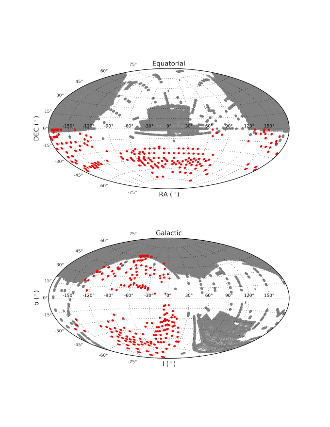
Figure 1: Aitoff projections of the SDSS footprint (gray) and the AEGIS footprint (red) in the equatorial coordinate system (upper panel) and in the Galactic coordinate system (lower panel).

The AEGIS survey is a medium-resolution ($R\sim$1,300) spectroscopic survey in the Southern Hemisphere, with the goal to determine the chemistry and kinematics of thick-disk and halo stars in order to constrain the chemodynamical evolution of the Milky Way. The input catalog for the spectroscopic targets was derived from photometric observations of a set of approximately 2-degree diameter fields taken during commissioning of the SkyMapper telescope (Keller et al., 2007). The gravity and metallicity sensitivity of the SkyMapper photometric system (Keller et al., 2007) allowed the focus of the target catalog to be on blue horizontal-branch, red clump, and metal-poor star candidates. The AEGIS sample excludes the region of sky within a 10 deg radius of the Galactic Center, and, in addition, a small number of candidate extremely metal-poor stars that formed the basis for a separate follow-up program (e.g., Jacobson et al., 2015).

Spectroscopic observations were carried out using the AAOmega multi-fibre dual-beam spectrograph (e.g., Sharp et al., 2006) on the 3.9m Anglo-Australian Telescope (AAT). Spectra were obtained for a total of $\sim$70,000 stars distributed over 4,900 square degrees of the southern sky during the four semesters of allocated time. All the survey observations were run through a uniform data reduction process based on the 2DFDR reduction code. Here we make use of the blue-arm spectra which, with the 580V grating, yields a wavelength coverage of approximately $\lambda$3750-5400 Å  and a resolving power $R\approx$ 1,300. A more complete description of the AEGIS data, sample spectra, and the analysis techniques used to derive the atmospheric parameters, as well as estimates of the [C/Fe] ratios and (photometric) distances, is provided in the Appendix.

Figure 1 compares the footprints on the sky of stars observed during SDSS/SEGUE and AEGIS. The sky coverage for SDSS/SEGUE was nearly contiguous over large portions of the sky, due to the numerous calibration stars (photometrically selected to be likely metal-poor main-sequence turnoff stars) observed during the extragalactic programs carried out during operation of the SDSS. The AEGIS footprint is rather sparse, but it covers the regions that SDSS could not reach.

Figure 2: Cartographic maps of carbonicity (upper panels) and metallicity (lower panels) projected onto the X-Z plane. The adopted Cartesian reference system is right-handed, having positive X towards the anti-center of the Galaxy. The location at (0,0) kpc corresponds to the center of the Galaxy, and the Sun is located at (X, Z) = (8.0, 0.0) kpc. The left panels show the distribution of stars in the X-Z plane in a square grid of 0.5 kpc $\times$ 0.5 kpc pixels. The filled squares have pixels with at least three stars and the filled dots indicate pixels with two or one stars. The right panels show the stellar distributions in the pixel grid smoothed with a two-pixel Gaussian kernel. The colors in the upper panels and the bottom panels represent the median [C/Fe] and [Fe/H] values at each pixel, respectively, as shown by the color bar under each panel. The upper and lower limits shown in the color bar are also used for pixels whose [C/Fe] or [Fe/H] lie above or below these limits. The gray-shaded area indicates the thick-disk region (TDR). The black- and red-dashed circles represent the dividing lines for the inner-halo (IHR), the transition region (TrR), and the outer-halo (OHR), based on the distribution of carbonicity. See text for the definition of these regions.

Figure 3: Cartographic maps of carbonicity (upper panels) and metallicity (lower panels) projected onto the Galactocentric Y-Z plane. The symbols and color scales are the same as in Figure 2.

3 Galactic Cartography of Carbonicity and Metallicity

Figure 4: Cartographic maps of carbonicity (upper panels) and metallicity (lower panels) projected onto the Galactocentric X-Y plane. The symbols and color scales are the same as in Figure 2. Stars in the thick-disk region (TDR: —Z— $\leq 3$ kpc) are removed from this plot.

Figures 2-4 are Galactocentric cartographic maps (projected onto the X-Z, Y-Z, and X-Y planes, respectively, in right-handed rectangular Galactocentric coordinates, having positive X towards the Galactic anti-center) of carbonicity (upper panels) and metallicity (lower panels). The left panels in each figure show the distribution of stars in a square grid of (0.5 kpc $\times$ 0.5 kpc) pixels. The filled squares have pixels with at least three stars, and the filled dots indicate pixels with two or one star. The right panels of each figure show the stellar distribution in the pixel grid, smoothed with a two-pixel Gaussian kernel. The color bar under each panel corresponds to the median values of the [C/Fe] and [Fe/H] values shown in the maps.

3.1 Galactic Components Based on Carbonicity

In order to identify individual Galactic components, and to consider the nature of the [C/Fe] and [Fe/H] distributions within them, we follow the approach of Lee et al. (2017), who made use of carbonicity to make these assignments (rather than metallicity or kinematics), with a few adjustments. For example, Lee et al. constructed dividing lines based on the cylindrical Galactocentric R-—Z— plane, whereas, in this work, we mapped the distributions of [C/Fe] and [Fe/H] projected onto the three rectangular Galactocentric planes (X-Z, Y-Z, and X-Y).

Our divisions based on carbonicity, shown in Figures 2–4, are obtained as follows. Both the dashed circles are centered around the Solar Neighborhood, at R = 8 kpc, Z = 0 kpc (Bovy 2015; for convenience, we used Z = 0 kpc rather than Z = 0.025 kpc), and the inner black and outer red circles have radii of 10 kpc and 15 kpc, respectively. The inner and outer circles correspond to the median value of [C/Fe] $\sim+0.2$ and [C/Fe] $\sim+0.4$ to +0.5, respectively. (We note that Lee et al. used [C/Fe] $\sim$ +0.4 and +0.6 for separating the halos, resulting in dividing circles located at R $\sim$ 8 kpc and 10 kpc respectively. These differences with respect to Lee et al. (2017) are purely data-driven; Lee et al. only made use of SDSS/SEGUE main sequence turn-off stars, while we employed stars over a wider range of luminosity in the AEGIS data, including more distant giants.) We then divided each map into four Galactic components, a thick-disk region (TDR; gray-shaded area, —Z— $\leq 3$ kpc, roughly three thick-disk scale heights above the Galactic plane), an inner-halo region (IHR; —Z— $>3$ kpc and inside the black-dashed circle), a transitional region (TrR; —Z— $>3$ kpc and between the dashed circles), and an outer-halo region (OHR; —Z— $>3$ kpc and outside the red-dashed circle). The individual components are labeled in the figures. Each region is dominated by stars in the indicated component population, yet still suffers contamination from other components, as described in detail in the next subsection. We note that, although the divisions we made are based on carbonicity, they are similar to previously suggested dividing lines for the IHR, TrR, and OHR based on either kinematics or metallicity (e.g., Carollo et al., 2007, 2010; de Jong et al., 2010; Tissera et al., 2014; Bland-Hawthorn & Gerhard, 2016, and references therein).

3.2 Metallicity Distributions in the Galactic Components

The Galactic components identified based on their carbonicity levels clearly correspond to different mean metallicities. As seen in the metallicity maps, the IHR exhibits a value near [Fe/H] $\sim-$1.5, while the OHR exhibits $-2.5<$ [Fe/H] $<-2.0$, on average. Figure 5 shows the MDFs, the carbonicity distribution functions, and the absolute carbon abundance distributions in the left, middle, and right panels, respectively. From top to bottom, the columns of panels indicate the TDR, IHR, TrR, and OHR regions, respectively. The gray-shaded histogram indicates all stars in the sample. The magenta and green histograms represent dwarf/turn-off (D/TO) stars and subgiant/giant (SG/G) stars, respectively. We note that there are a small fraction of D/TO stars in the OHR, which are likely to be spurious. We left out these D/TO stars in the green histogram representing the OHR in the bottom panels. The green-, blue-, and red-dashed vertical lines represent the mean metallicity ([Fe/H] = $-$0.6, $-$1.6, and $-$2.2) of the thick-disk, inner- halo, and outer-halo populations, respectively (see, e.g., Carollo et al. 2010 and An et al. 2013). Details of the metallicity distributions for the stars in each region are provided below.

1. Thick-Disk Region (TDR) – The peak metallicity of the stars in this region is located at [Fe/H] $\sim-$0.7, and this region is likely dominated by stars of the thick-disk population. A large fraction ($\sim$74%) of the population in the sample consists of dwarfs and turn-off stars, unlike the other three components, which are predominantly sub-giants or giants. The peak metallicity of the D/TO MDF is [Fe/H]$\sim-$0.7, commensurate with many studies (Carollo et al., 2010; An et al., 2013), while the SG/G stars exhibit a peak metallicity at [Fe/H]$\sim-$1.4, and may suffer from contamination from the inner-halo population (IHP).

2. Inner-Halo Region (IHR)– The dominant population is comprised of sub-giants and giants with a peak metallicity at [Fe/H] $=-$1.6, which is clearly distinct from the thick disk.

3. Transitional Region (TrR) – Sub-giants and giants are dominant in this region as well, and they reflect a mixture of the IHP at [Fe/H] $=-$1.6 and the outer-halo population (OHP) at [Fe/H]$=-$2.2.

4. Outer-Halo Region (OHR)– The sub-giants and giants that dominate this region include contributions from both the IHP and OHP. The tail of lower-metallicity stars in the MDF is clearly stronger than for the other regions.

The enumerated results above for the stellar populations represented in the Galactic components are quite similar to those obtained from the main-sequence turn-off stars from SDSS studied by Lee et al. (2017). As in that work, it is interesting to see that the Galactic components identified by carbonicity cuts provide independent evidence for the existence of the Galactic components in metallicity space.

3.3 Distribution of Carbon in the Galactic Components

The middle panels of Figure 5 indicate that the level of carbonicity increases with decreasing metallicity from the TDR to the OHR, as shown in the cartographic maps. The fraction of stars with higher carbonicity increases from the TDR to the OHR as well.

The $A$(C) distribution (shown in the right-hand panels) in each component also shifts toward lower values from the TDR to the OHR. The dominant population of D/TO stars in the TDR have a peak at $A$(C) $\sim$ 7.8, while the SG/G population exhibits a peak at $A$(C) $\sim$ 7.0, a difference of $\sim$ 0.8 dex. This can be accounted for by the difference in metallicity between the D/TO stars and the SG/G stars (both having [C/Fe]$\sim$ 0.0), due to the different sampling of the populations resulting from the higher luminosities of the SG/G stars.

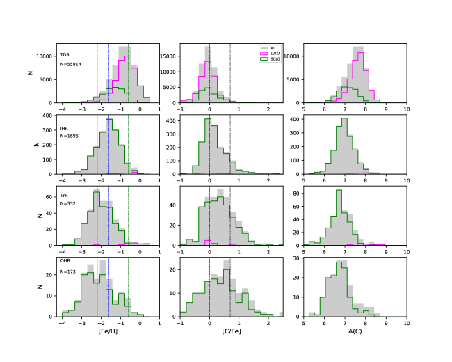
Figure 5: Distributions of metallicity (left panels), carbonicity (middle panels), and absolute carbon abundance (right panels). The carbonicity estimates were corrected for SG/G stars by adopting the evolution-correction calculation of Placco et al. (2014). The top to bottom panels indicate the TDR, IHR, TrR, and OHR, respectively. The gray-shaded, magenta-solid, and green-solid histograms represent all stars including FHB stars, D/TO stars only, and SG/G stars only, respectively. The total number of stars in each Galactic component is reported underneath each component designation in the left panels. The red-, blue-, and green-dashed vertical lines represent the mean metallicity of the outer halo, inner halo, and thick disk, respectively (Carollo et al., 2010). The black-dashed lines in the middle panels indicate [C/Fe] = 0.0 and [C/Fe] = +0.7.

4 Carbon-Enhanced Metal-Poor Stars in the AEGIS Sample

4.1 The CEMP Population

We now explore the properties of the CEMP stars present in the AEGIS sample. As seen in the middle panels of Figure 5, the fraction of CEMP stars increases from the TDR to the OHR, although only about 3% of the AEGIS sample are CEMP stars. The TDR has a negligible fraction of CEMP stars, since most are D/TO stars, whose higher effective temperatures make identification of CEMP stars difficult (Lee et al., 2013; Placco et al., 2014, 2016a). However, moving from the IHR to the OHR reveals a substantial increase in the fractions of CEMP stars. There are a total of 1,691 CEMP stars in the AEGIS sample, comprising 1,109 SG/G stars, 433 D/TO stars, and 149 field horizontal-branch stars. Here we only consider the SG/G and D/TO stars, resulting in a total of 1,542 CEMP stars for the classification and frequency analysis described below.

Figure 6: Panels (a) and (b) show the cumulative frequencies at a given metallicity and the differential frequencies of CEMP SG/G stars at each metallicity bin, respectively. Panels (c) and (d) represent the cumulative frequencies and differential frequencies of the CEMP-no and CEMP-$s$ stars, respectively. Frequencies are calculated relative to all SG/G stars. In panel (a), the green-dotted line represents the cumulative frequency based on the observed carbon abundances, and the solid lines in all four panels show that the frequencies taking account of the carbon-abundance corrections from Placco et al. (2014). The green-, blue-, and red-solid lines represent the frequencies of all CEMP stars regardless of their sub-classes, CEMP-no only, and CEMP-$s$ only stars, respectively. The lightly colored shaded areas around the solid lines indicate 1$\sigma$ CI_W of individual frequencies. The black-filled circles with error bars in panels (a) and (b) indicate the frequencies of SDSS/SEGUE CEMP stars from Lee et al. (2013). The gray lines in panels (c) and (d) represent the high-resolution sample of CEMP-no stars from Placco et al. (2014). Details can be found in the text.

4.2 CEMP Classifications

It is important, where possible, to distinguish between the sub-classes of CEMP stars, as each may correspond to a different class of stellar progenitor(s), and explore different epochs of the assembly and chemical evolution of the Galaxy (e.g., Hansen et al., 2016a). Until quite recently, it was thought that such classification required high-resolution spectroscopy, in order to detect the heavy elements Ba and Eu that form the basis of the sub-class assignments as described by Beers & Christlieb (2005). However, based on a large sample of CEMP stars with available high-resolution spectroscopic classifications, Yoon et al. (2016) demonstrated that CEMP-no stars (whose surface abundances are believed to be reflect the gas from which they formed, Hansen et al. 2016b) could be reasonably well-distinguished from the class of CEMP-$s$ stars (whose surface abundances reflect a mass-transfer event from a former AGB companion) on the basis of their absolute carbon abundances alone, without the use of high-resolution spectroscopy. According to the Yoon et al. study, their method employing $A$(C) enabled classification of CEMP stars with $A$(C) ¿ 7.1 as CEMP-$s$ stars and those with $A$(C) $\leq$ 7.1 as CEMP-no stars, with a success rate of $\sim$ 90%. In the following analysis, it is understood that the CEMP-$s$ and CEMP-no stars are classified as such through application of this approach.

While the stars under consideration by Yoon et al. (2016) were primarily sub-giants and giants, Lee et al. (2017) explored the $A$(C) distribution of $\sim$ 100,000 main sequence turn-off (MSTO) stars from SDSS/SEGUE. They claimed that the MSTO stars require a different (higher) dividing line on absolute carbon abundance, $A$(C) = 7.6, since in their temperature range (5600 K $\leq$ $T_{\rm eff}$ $<$ 6700 K) carbon molecular features become substantially weaker; identification of CEMP stars becomes increasingly difficult unless they have quite high carbonicity. If we use $A$(C) = 7.6 as the dividing line for D/TO stars in the AEGIS sample, we identify 166 CEMP-no stars and 267 CEMP-$s$ stars; using $A$(C) = 7.1 for SG/G stars, we identify 527 CEMP-no stars and 582 CEMP-$s$ stars.

5 Frequencies of the CEMP stars

The frequencies of CEMP stars as a function of metallicity provide strong constraints on GCE (e.g., Kobayashi et al., 2011; Côté et al., 2016; Salvadori et al., 2016), the assembly history of the Galaxy (e.g., Carollo et al. 2012, 2014), and potentially on the First Initial Mass Function (FIMF; e.g., Lucatello et al., 2006; Tumlinson, 2007; Suda et al., 2013; Carollo et al., 2014; Yoon et al., 2016; de Bennassuti et al., 2017; Ishigaki et al., 2018). They also constrain the different channels for formation of carbon-rich vs. carbon-normal stars at low metallicity (Norris et al., 2013; Placco et al., 2014; Chiaki et al., 2017).

In constructing CEMP frequencies for the AEGIS sample, we have made a few assumptions, enumerated below.

1. Determining reliable chemical abundances of cool, strongly carbon-enhanced, low-metallicity stars is very challenging, since the strong molecular carbon bands can significantly depress the continuum level. We thus limit our consideration to stars with effective temperatures $T_{\rm eff}>4000$ K.

2. Due to the difficulty of identifying the carbon enhancement for warmer stars, we have limited our consideration of frequencies to the SG/G stars in the AEGIS sample. We note from the discussion above that the SG/G stars are the dominant population in the halo system (both for the inner halo and the outer halo).

3. Since we only include the SG/G stars, we have used $A$(C) = 7.1 for separating CEMP-no stars from CEMP-$s$ stars, as in Yoon et al. (2016).

Figure 6 shows the resulting derived frequencies, as a function of [Fe/H], for the CEMP stars in the AEGIS sample. This figure shows four panels of frequencies defined as follows; (a) cumulative frequencies of all CEMP stars (regardless of their sub-class), (b) differential frequencies of all CEMP stars, (c) cumulative frequencies of each CEMP sub-class (CEMP-no and CEMP-$s$ plotted separately), and (d) differential frequencies of each CEMP sub-class. In all cases the definition [C/Fe] $\geq+0.7$ was used for identification of CEMP stars in the AEGIS sample. The dotted line in panel (a) represents the cumulative frequency of all CEMP stars using the derived carbon abundances from the n-SSPP, which can reflect diluted abundances for evolved stars due to first dredge-up. The green-, blue-, and red-solid lines in Figure 6 represent the results based on application of the carbon correction procedure of Placco et al. (2014) for all CEMP, CEMP-no, and CEMP-$s$ stars from the AEGIS survey, respectively. The light-green, light-blue, and light-red shaded areas represent the Wilson score confidence intervals (CI_W; Wilson 1927). For comparison, the black circles in panel (a) represent the cumulative frequencies for stars with [C/Fe] $\geq$ +0.7 from the SDSS/SEGUE data of Lee et al. (2013). Note that Lee et al. made use of stars with 4400 K $<$ $T_{\rm eff}$ $<$ 6700 K, S/N $\geq$ 20.0, and all luminosity classes (D, TO, SG, and G). The SDSS/SEGUE differential frequencies for the CEMP stars (black circles) are included for comparison in panel (b). The SDSS/SEGUE frequencies include all classes of CEMP stars (there was no mechanism to differentiate sub-classes at the time), as well as all stars in the various luminosity classes. The bottom two panels (c) and (d) include the frequencies, calculated from the extensively compiled dataset of the CEMP-no stars, carried out with high-resolution spectroscopy (Placco et al., 2014) for comparison with the AEGIS CEMP-no sample. It is clear that the CEMP frequency estimate based on the SDSS/SEGUE data is substantially lower than the CEMP-no star frequencies in the AEGIS sample, and higher than the CEMP-$s$ star frequencies seen in panels (c) and (d).

We draw the following inferences from inspection of Figure 6.

1. The difference between the green-solid line and green-dotted line in panel (a) of Figure 6 shows that it is necessary to include the evolutionary corrections for carbon dilution, as it changes the estimates by on the order of 10-30%, depending on the metallicity.

2. The cumulative frequencies (the green lines) of the CEMP stars in panel (a) increase with decreasing metallicity, as has been reported by previous studies. However, since Lee et al. (2013) included both D/TO and SG/G stars in their counts (denominator as well as numerator), and did not correct the carbon abundances according to evolutionary status for their frequency calculation, their final frequencies (the black line with dots) ended up being about a factor of two smaller than our result (the green-solid line). We attribute this result to both the uncorrected carbon abundances and the difficulty of identifying CEMP stars (in particular for CEMP-no stars, due to their substantially lower $A$(C) at a given [C/Fe]) for warmer stars, effectively removing true CEMP stars from the numerator, and the addition of a substantially larger fraction of D/TO stars, relative to SG/G stars, to the denominator.

3. As seen in panel (b) of Figure 6, the differential frequencies of the CEMP stars from the SDSS/SEGUE and the AEGIS sample both increase with decreasing metallicity. However, as for the cumulative frequencies noted above, the Lee et al. (2013) differential frequencies for the SDSS/SEGUE sample are substantially lower than found for the AEGIS sample, due to the uncorrected carbon abundances and the different luminosity classes that were included in the counting exercise.

4. Both the cumulative and differential frequencies of the CEMP-no stars steeply increase with decreasing metallicity, as seen in panels (c) and (d). Since there was no way to differentiate CEMP sub-classes for the SDSS data (at that time), we cannot directly compare our result with the SDSS data frequencies (Lee et al., 2013). However, the frequencies based on high-resolution data for the CEMP-no stars (Placco et al., 2014) clearly support not only our calculation of the frequencies, but also tacitly validate that the $A$(C) classification method is as effective as that of the conventional [Ba/Fe] criterion, even though there are some small differences in the fractions shown in panels (c) and (d). We also note that this consistency of the frequencies is likely to arise from the fact that the high-resolution sample predominantly comprises sub-giants and giants, unlike the SDSS data reported by Lee et al. (2013).

5. In panels (c) and (d), our tiny sample of stars with [Fe/H]$\leq-$4.0 has a 100% (with a 1$\sigma$ CI_W of 20%) frequency of CEMP-no stars (4 out of 4 stars in the metallicity bin; one star is a Group III star and three are Group II stars, according to the criteria of Yoon et al. 2016). We note that there are more stars in these two groups with [Fe/H] $>-$4.0. However, there is a transitional region ($-3.5<$ [Fe/H]$<-2.5$ and $A$(C)$<$7.1), where both Group II and Group III stars reside; higher-resolution spectroscopy of $A$(Mg) and/or $A$(Na) is required for clear separation in this metallicity range.

6. A transition in the dominant stellar population from CEMP-$s$ stars to CEMP-no stars with decreasing metallicity is clearly seen at [Fe/H]$\sim-2.3$ in panel (d).

7. Both the cumulative and differential frequencies of the CEMP-$s$ stars in the panels (c) and (d) are flat ($\sim$10%) for the stars with [Fe/H] $\lesssim-2.0$, consistent with the CEMP frequency at [Fe/H] $\sim-$2.3 obtained by Abate et al. (2015) (between 7% and 17%). Their CEMP frequency was based on their synthetic stellar-population models (which only included binary mass-transfer origins for CEMP stars) and then compared with the observed CEMP fractions for SDSS/SEGUE stars from Lee et al. (2013). They found an inconsistent result, that their theoretical CEMP fraction was a factor of two lower than that of the observed data. The reason for this discrepancy is now made clear; at low metallicities, the CEMP-$s$ stars must be separated from the increasingly common CEMP-no stars prior to the comparison being made.

6 Discussion

The formation of the Galaxy and its chemical-evolution history are closely interconnected. In particular, the spatial distribution of the stellar chemical elements in different regions provides information not only on the various stellar populations, but also on their natal environments, which helps to constrain their stellar progenitors. Here we have used a new large sample of medium-resolution spectra for stars in the Southern Hemisphere, the AEGIS survey, to explore the spatial distributions of C and Fe, and consider the frequencies of CEMP stars. For the first time, we have been able to sub-classify the stars into CEMP-no and CEMP-$s$ stars, using medium-resolution spectra alone. These results are discussed below, in the context of the dual halo model of the Milky Way.

6.1 The Dual Halo System as Revealed by Carbonicity

Lee et al. (2017) constructed the first carbonicity maps of the Galactic halo, based on a large sample of MSTO stars from SDSS/SEGUE. Their carbonicity map indicated a clear dichotomy of the halo system in terms of the relative fractions of the two most populous CEMP sub-classes – the low $A$(C) stars associated with CEMP-no stars were found to dominate the OHR, while the high $A$(C) stars associated with CEMP-$s$ stars dominate the IHR. This result provided support to the initial claim for this segregation made by Carollo et al. (2012), based on a much smaller sample of CEMP-no and CEMP-$s$ stars classified on the basis of available high-resolution spectroscopy.

Following the Lee at al. prescription to divide the halo system based on its distribution of carbonicity, inspection of the relative fractions of CEMP-no and CEMP-$s$ stars in the AEGIS survey (considering only the SG/G stars) revealed a similar behavior. The IHR comprises 47$\pm$4% CEMP-no stars and 53$\pm$4% CEMP-$s$ stars, the TrR comprises 64$\pm$6% CEMP-no and 36$\pm$6% CEMP-$s$ stars, and the OHR comprises 78${}^{+6}_{-8}$% CEMP-no and 22 ${}^{+6}_{-8}$% CEMP-$s$ stars; errors in the frequencies were calculated based on the 1$\sigma$ CI_W. Although the fractions of the sub-classes differ somewhat from those found by Lee et al., the dominant population in each Galactic component is consistent with their result.

Both the Lee et al. results and ours can be understood in terms of our current picture of the formation of the inner- and outer-halo populations of stars (summarized in the next sub-section). The relatively more massive ($\sim 10^{9}$M_⊙) mini-halos (classical dwarf galaxy counterparts) that formed the IHP led to the production of larger fractions of CEMP-$s$ stars that dominate the IHR, while the relatively less massive ($\sim 10^{6}$M_⊙) mini-halos (ultra-faint dwarf galaxy counterparts) that were accreted to form the OHP led to larger fractions of CEMP-no stars in the OHR. The MDFs of low-mass mini-halos, on average, span a broader [Fe/H] range, with much lower metallicity tails, than more massive mini-halos, due to their truncated star-formation history. Thus they contain more of the most metal-poor stars with [Fe/H]$<-$3.0, which are predominantly CEMP-no stars. However, massive mini-halos have more metal-rich stars, due to more prolonged star formation, thus we expect the CEMP-$s$ stars to dominate over the CEMP-no stars in these environments (Salvadori et al., 2015, 2016).

6.2 Galactic Formation History as Revealed by Metallicity

Eggen et al. (ELS; 1962) proposed a rapid monolithic collapse model of the Galactic halo, which was later challenged by Searle & Zinn (SZ; 1978), who claimed that the formation of the halo was due to the accretion of “protogalactic fragments” that continued to fall into the Galaxy after formation of the central region was complete. Aspects of both the ELS model and the SZ model were reflected in subsequent observational work and simulations, which converged to favor the halo accretion model (e.g., Samland & Gerhard, 2003; Steinmetz & Muller, 1995; Chiba & Beers, 2000; Bekki & Chiba, 2001; Brook et al., 2003; Bullock & Johnston, 2005; Diemand et al., 2005; Zolotov et al., 2009).

More recent studies, using large samples of stars from SDSS/SEGUE, were able to demonstrate the existence of at least two distinct stellar halos – the inner halo and the outer halo – based on the spatial distributions of metal-poor stars, and correlations between with kinematics and metallicity (e.g., Bekki & Chiba, 2001; Carollo et al., 2007; De Lucia & Helmi, 2008; Carollo et al., 2010; de Jong et al., 2010; Beers et al., 2012; Xu et al., 2018, and references therein). The flattened IHR is dominated by contributions from the IHP at distances $\leq$ 10-15 kpc, while the more spherical OHR is dominated by contributions from the OHP beyond 15-20 kpc. As supported by more recent numerical simulations (e.g., Amorisco, 2017; Starkenburg et al., 2017), the outer halo is likely to have formed via essentially dissipationless accretion of low-mass mini-halos, whereas the inner halo formed via dissipative merging between more-massive mini-halos.

The dual halo components selected by applying the carbonicity cuts in both the Lee et al. and the AEGIS sample are clearly well-represented as distinct peaks in the MDFs of the stars in the IHR and OHR, at [Fe/H] $\sim-$ 1.6 and $-$ 2.2, commensurate with the results of previous studies based on the density distribution and kinematics of halo stars (e.g., Carollo et al., 2010; Beers et al., 2012; An et al., 2013, 2015; Das & Binney, 2016).

6.3 Constraints from the Frequencies of CEMP Stars

The frequencies of CEMP stars have been considered in a number of previous studies based on a variety of samples (Cohen et al., 2005; Lucatello et al., 2006; Frebel et al., 2006; Carollo et al., 2012; Lee et al., 2013; Placco et al., 2014; Beers et al., 2017), all of which concluded that the cumulative frequency of CEMP stars strongly increases with decreasing metallicity. However, our present analysis differs in that we have limited our calculations to consider only SG/G stars, due to the recognition that including the (generally warmer) D/TO stars leads to a distortion of the true frequencies. The combined effects of the difficulty of detecting carbon enhancement for warmer stars and the fact that there exist several orders of magnitude difference in the $A$(C) for CEMP Group I stars vs. CEMP Group II and III stars seen in the Yoon-Beers diagram confounds the naive calculation of frequencies which ignore them. The net result is to lower (by up to a factor of two) the reported frequencies of CEMP stars from their correct values. Secondly, we have reported here, for the first time, the cumulative and differential frequencies of individual CEMP sub-classes (CEMP-no and CEMP-$s$). Because these sub-classes have different astrophysical origins, it is necessary to distinguish them in order to place reliable constraints on chemical-evolution and stellar population-synthesis modeling.

Important implications can be drawn from inspection of the individual frequencies for CEMP-no and CEMP-$s$ stars, summarized below:

1. The CEMP-no fraction in the extremely low-metallicity regime ([Fe/H] $<-3.0$) is sensitive to the FIMF and to the yields of the first enrichment sources, since these stars are expected to be bona-fide second-generation stars (e.g., Placco et al., 2015; Hansen et al., 2016b; Placco et al., 2016b; Yoon et al., 2016; Sharma et al., 2017, and reference therein).

2. The differential and cumulative frequencies of the CEMP-$s$ stars, when considered alone, are substantially lower than the frequencies of all CEMP stars. The discrepancy between the observed frequencies of SDSS CEMP stars (Lee et al., 2013) at low metallicity (when considered as a single population) with the predicted frequencies from population-synthesis models that only included binary mass-transfer origins (Abate et al., 2015) has now been removed. The reason can be explained as follows. Lee et al. (2013) did not have a method to separate the CEMP-$s$ stars from the CEMP-no stars at the time, so their estimated CEMP fraction included both sub-classes. However, most CEMP-$s$ stars have a binary mass-transfer origin, thus the proper comparison should be between the Abate et al. prediction and and the observed CEMP-$s$ fraction, which has been carried out in this work.

3. The apparently constant differential fraction ($\sim 10$%) of the CEMP-$s$ stars at $-4.0\,\lesssim$ [Fe/H] $\lesssim-$ 2.0 suggests that metallicity does not have a significant influence on the operation of the $s$-process, on the formation of low-mass binaries, or on their initial separation, all of which might have impacted the observational result. According to Yoon et al. (2016), there exist a substantial number of CEMP-$s$ stars at [Fe/H] $<-$3.0 – there are even two CEMP-$s$ stars known with [Fe/H] $<-$3.5: CS 22960-053 with [Fe/H] $=-$3.64 (Roederer et al., 2014) and HE 0002-1037 with [Fe/H] $=-$3.75 (Hansen et al., 2016c). The apparent cut-off metallicity at [Fe/H]$\sim-$3.8 may indicate that the emergence of AGB stars was delayed to accommodate the evolutionary timescales for intermediate-mass stars, but the numbers are still too small be to clear on this point.

   For completeness, we note that spinstar production of $s$-process elements at extremely low metallicity, which would not necessarily require a mass-transfer event, has been suggested by several authors (e.g., Frischknecht et al., 2016; Choplin et al., 2017) to account for the possible non-binary nature of several CEMP-$s$ stars reported by Hansen et al. (2016c). Larger samples of CEMP-$s$ stars with [Fe/H] $<-3.0$ with available high-resolution spectroscopic analyses, as well as more extensive radial-velocity monitoring, are required to evaluate these predictions.

4. The transition of the dominant CEMP sub-class from CEMP-no stars to the CEMP-$s$ stars appears at [Fe/H] $\sim-2.3$. This can be interpreted as the transition from a FIMF (favoring more-massive-stars) to the current IMF (favoring low- and intermediate-mass stars), as discussed previously by Suda et al. (2011), Suda et al. (2013), Yamada et al. (2013), and Lee et al. (2014).

   Interestingly, the fractions of the CEMP-no and CEMP-$s$ stars we obtain over the metallicity range considered in our sample ($-4.0<$ [Fe/H] $<-$1.0) are roughly similar, in contrast to previous suggestions that the CEMP-$s$ stars are the dominant population (e.g., Aoki et al., 2007). This discrepancy likely arises due to the low $A$(C) associated with the CEMP-no stars, so that they were not recognized as CEMP stars at the main-sequence turnoff, unlike the high-$A$(C) CEMP-$s$ stars.

7 Summary and Future Work

We have explored the AEGIS sample, an extensive spectroscopic data set ($\sim$58,000 stars) in the Southern Hemisphere, to study the origin and formation history of the Galactic halo, and its chemical evolution, by considering the spatial distributions of [C/Fe] and [Fe/H], the stellar populations, and CEMP-star frequencies. We have confirmed that carbonicity increases and metallicity increases with distance, from the IHR to the OHR. Based on the CEMP population in the halo systems present in the AEGIS sample, we also confirm the previous results that the CEMP-$s$ stars are dominant in the IHR, while the CEMP-no stars dominate the OHR. Both the cumulative and differential frequencies of CEMP stars increase with decreasing metallicity.

For the first time, we calculated the separate frequencies of CEMP-no and CEMP-$s$ stars, based on medium-resolution spectroscopy alone, making use of their characteristically different $A$(C) values, as described by Yoon et al. (2016). The frequencies of the CEMP-no stars are consistent with the result obtained from the extensive compilation of high-resolution data for CEMP-no stars explored by Placco et al. (2014). The frequencies of the the CEMP-$s$ stars are almost constant with declining metallicity, at about 10%, consistent with the result of Abate et al. 2015 from population-synthesis modeling assuming only binary mass-tranfer origins for CEMP stars.

To complete this effort, we are planning to re-calculate the frequencies of CEMP-no and CEMP-$s$ stars from SDSS/SEGUE data based on sub-giants and giants alone, and carry out kinematic analyses of CEMP-no/CEMP-$s$ stars from AEGIS, SDSS/SEGUE, and RAVE, in particular with more accurate distances and proper motions from Gaia DR2. Comparison of these observations with the predicted frequencies of CEMP-no and CEMP-$s$ stars as a function of metallicity, and the expected morphology of the $A$(C) vs. [Fe/H] diagram of Yoon et al. (2016), based on different input parameters for cosmological hydrodynamical simulations (as recently explored by Sharma et al. 2017 and Hartwig et al. 2018), could provide powerful new constraints on the nature of star formation and chemical evolution in the early universe. In the near future, we expect to be able to identify numerous CEMP Group II and III stars, based on the morphology of the $A$(C) vs. [Fe/H] space, and advance our understanding about the origin and nature of the first generations of stars in the universe.

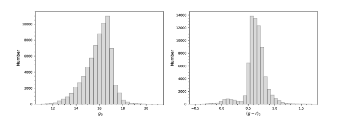
Figure 7: Distributions of $g_{0}$ and $(g-r)_{0}$

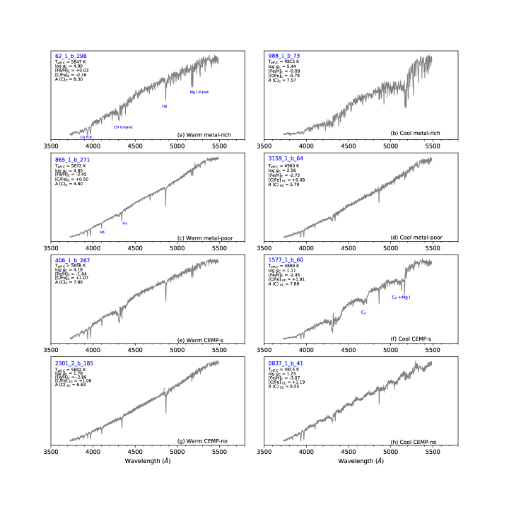
Figure 8: Example AEGIS spectra. Upper row: Spectra of relatively warm (left panel) and cool (right panel), metal-rich, carbon-normal stars. Second row: Spectra of relatively warm (left panel) and cool (right panel), metal-poor, carbon-normal stars. Third row: Spectra of relatively warm (left panel) and cool (right panel) CEMP stars classified as CEMP-$s$, based on the $A$(C) criterion. Bottom row: Spectra of relatively warm (left panel) and cool (right panel) CEMP stars classified as CEMP-no, based on the $A$(C) criterion.

Here we summarize the nature of the AEGIS sample, provide examples of the spectra obtained, and describe the analysis procedures used for the derivation of the atmospheric parameters ($T_{\rm eff}$, $\log g$, and [Fe/H]), as well as the carbon-to-iron ratio (carbonicity), [C/Fe]. We also summarize the procedures used for the distance estimates employed.

Appendix A The AEGIS Sample

The original photometry is obtained from commissioning era SkyMapper observations (Wolf et al., 2018). Transformations from the observed $g$ magnitudes and $g-r$ colors (obtained from a calibration of $g-i$ colors to $g-r$ from APASS (Henden et al., 2015; Wolf et al., 2018) were applied. Reddening estimates were taken from Schlegel et al. (1998). Figure 7 shows the distribution of $g_{0}$ and $(g-r)_{0}$ for the stars in the AEGIS sample. The brightest stars reach $g_{0}\sim 11.5$, while the faint limit of stars with available spectroscopy is $g_{0}\sim 20$ but the vast majority of are brighter than $g_{0}\approx$ 18.

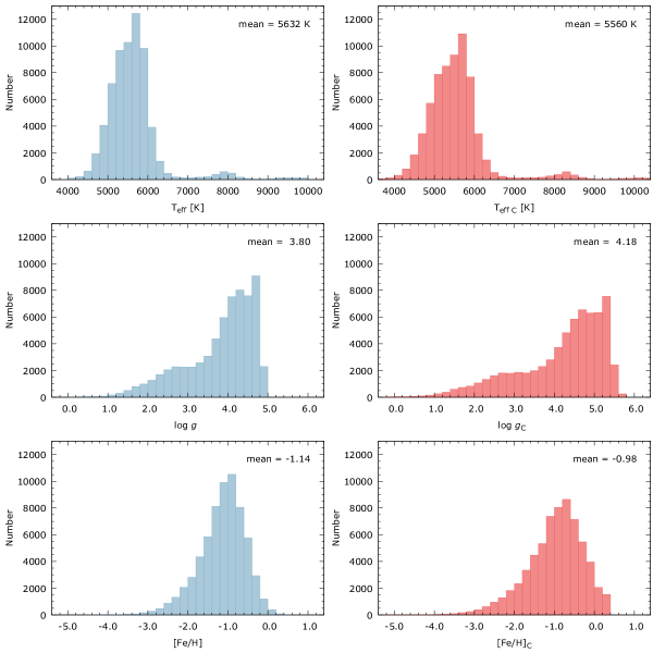
Figure 9: Distributions of derived atmospheric parameters for the AEGIS sample. The left-hand panels correspond to the n-SSPP estimates of $T_{\rm eff}$, $\log g$, and [Fe/H], from top to bottom, respectively. The right-hand panels show the distributions of these estimates after transformation to a high-resolution spectroscopic scale ($T_{\rm eff\,C}$, $\log g_{\rm C}$, and [Fe/H]_C (see text).

The typical signal-to-noise of the blue spectra was $S/N\sim 50-55$, averaged over the full spectrum, which is sufficient to obtain atmospheric-parameter, carbonicity, and [$\alpha$/Fe] estimates. Figure 8 provides examples of typical medium-resolution $R\sim 1,300$ spectra for the AEGIS program stars, obtained with the blue arm of the AAOmega spectrograph, The panels in the left-hand column correspond to warmer stars ($T_{\rm eff}\sim 5800$ K), while the right-hand panels are cooler stars ($T_{\rm eff}\sim 4800$ K). The upper two rows of panels are relatively metal-rich and metal-poor carbon-normal stars, according to their estimates of [C/Fe]_C, (indicating a transformation to a high-resolution scale) or [C/Fe]_EC (indicating an additional application of the evolutionary carbon correction described by Placco et al. 2014, which only applies to giant stars; see below) respectively. The lower two rows are relatively metal-rich and metal-poor CEMP-$s$ ($A(C)_{\rm C}$ or $A$(C)_EC $>7.1$) and CEMP-no stars ($A(C)_{\rm C}$ or $A$(C)_EC $<7.1$), respectively. The final derived parameters are shown for each star in the legends, and prominent spectral features are labeled.

Appendix B Derivation of Atmospheric Parameters and [C/Fe]

Estimates of the stellar atmospheric parameters ($T_{\rm eff}$, $\log g$, and [Fe/H]), and [C/Fe] were determined by employing the n-SSPP pipeline (Beers et al., 2014, 2017), which is a “non-SEGUE” version of the SEGUE Stellar Parameter Pipeline (SSPP; see Lee et al., 2008a, b; Allende Prieto et al., 2008; Smolinski et al., 2011; Lee et al., 2011, 2013, for a detailed description of the procedures and calibrations used). The n-SSPP employs both spectroscopic and photometric ($V_{0},(B-V)_{0}$, here, obtained from $g_{0}$ and $(g-r)_{0}$ using the transformations of Zhao & Newberg 2006, and $J_{0}$ and $(J-K)_{0}$ from 2MASS; Skrutskie et al. 2006) information as inputs, in order to make a series of estimates for each stellar parameter. Then, using $\chi^{2}$-minimization matching techniques within dense grids of synthetic spectra, and averaging with other techniques as available (depending on the wavelength range of the input spectra; see Table 5 of Lee et al. 2008a), the best set of values is adopted. For application to the AEGIS data, the internal errors for the stellar parameters are typically 125 K for $T_{\rm eff}$, 0.25 dex for $\log g$, and 0.20 dex for [Fe/H] and [C/Fe].

Final corrections were applied to the n-SSPP-derived parameters to match a high-resolution spectroscopic scale, as described in Beers et al. (2014). For spectra with the quality of AEGIS data, the external precision of the n-SSPP estimates of $T_{\rm eff}$, log $g$, [Fe/H], and [C/Fe] is on the order of 150 K, 0.35 dex, and 0.25 dex, and 0.25 dex, respectively (Beers et al., 2014, 2017). As noted above, for giants, we also made corrections to the carbon-abundance estimates in order to restore the original amount of carbon in a star’s atmosphere prior to dredge-up on the giant branch during stellar evolution (Placco et al., 2014).

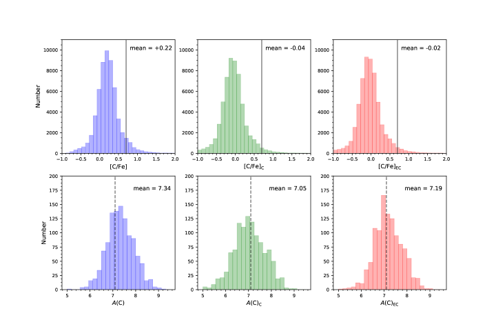
Figure 10: Distributions of derived carbon-abundance estimates for the AEGIS sample. The upper row shows the n-SSPP estimates of [C/Fe], [C/Fe]_C, after transformation to a high-resolution spectroscopic scale, and [C/Fe]_EC, after an additional correction of the giants for the dilution of carbon during first dredge-up, from left to right, respectively. The gray vertical solid line indicates the division of carbon-normal stars from CEMP stars at [C/Fe] = +0.7. The lower row shows the corresponding distribution of absolute carbon abundances $A$(C), $A$(C)_C, and $A$(C)_EC, from left to right, respectively (see text). The gray vertical dashed line indicates the division on $A$(C) used by Yoon et al. (2016) to differentiate CEMP-$s$ stars from CEMP-no stars at $A$(C) = 7.1. Note that only the CEMP SG/G stars from AEGIS are shown for the bottom panels (see text).

Although the n-SSPP also obtains estimates of [$\alpha$/Fe], they are not employed in the present study. Also, in this work we only consider stars with $T_{\rm eff\,C}>$ 4000 K, due to the difficulty of obtaining reliable parameters for these spectra in the presence of strong molecular bands. There were a total of 58,029 stars with suitable-quality spectra required to derive reliable stellar parameter estimates.

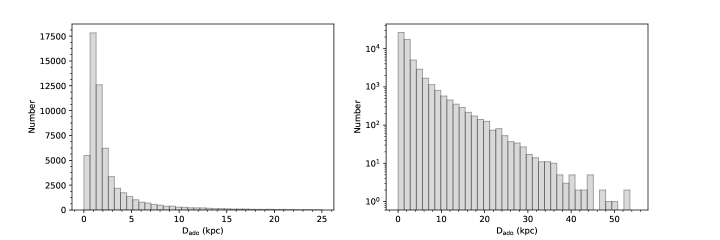
Figure 11: Distributions of the adopted (photometric) distance, D_ado. The left-hand panel shows a linear vertical scale, while the right-hand panel uses a log vertical scale.

Appendix C Derivation of Distance Estimates

Distances to individual stars are estimated using the distance modulus relationships between M_v and $(B-V)_{0}$ described by Beers et al. (2000). These relationships require the likely evolutionary status assigned by the n-SSPP to be specified, which is based on the derived surface gravity estimate. See Beers et al. (2012) for a complete discussion of this method. Based on previous tests of this approach, we expect the distances assigned as described above to be accurate to on the order of 15-20%. For production of the cartographic maps we only considered stars with available distance measurements, resulting in a total of 58,015 stars. Figure 11 shows the distribution of derived distance estimates for the AEGIS sample, using both a linear and a log vertical scale. From inspection of the figure, although AEGIS includes stars as distant as $\sim 50$ kpc, the great majority of the stars $\sim 85$ % are located within 5 kpc of the Sun; it is a relatively local sample.

The complete set of spectra and derived parameters for the AEGIS sample are being prepared for public release in due course.

References

- Abate et al. (2015) Abate, C., Pols, O. R., Izzard, R. G., & Karakas, A. I. 2015, A&A, 581, A22
- Abbott et al. (2017) Abbott, B. P., Abbott, R., Abbott, T. D., et al. 2017, ApJ, 848, L13
- Allende Prieto et al. (2008) Allende Prieto, C., Sivarani, T., Beers, T. C., et al. 2008, AJ, 136, 2070
- Amorisco (2017) Amorisco, N. C. 2017, MNRAS, 464, 2882
- An et al. (2015) An, D., Beers, T. C., Santucci, R. M., et al. 2015, ApJ, 813, L28
- An et al. (2013) An, D., Beers, T. C., Johnson, J. A., et al. 2013, ApJ, 763, 65
- Aoki et al. (2007) Aoki, W., Beers, T. C., Christlieb, N., et al. 2007, ApJ, 655, 492
- Aoki et al. (2013) Aoki, W., Beers, T. C., Lee, Y. S., et al. 2013, AJ, 145, 13
- Arcones & Thielemann (2013) Arcones, A., & Thielemann, F.-K. 2013, Journal of Physics G Nuclear Physics, 40, 013201
- Astropy Collaboration et al. (2013) Astropy Collaboration, Robitaille, T. P., Tollerud, E. J., et al. 2013, A&A, 558, A33
- Barklem et al. (2005) Barklem, P. S., Christlieb, N., Beers, T. C., et al. 2005, A&A, 439, 129
- Beers et al. (2000) Beers, T. C., Chiba, M., Yoshii, Y., et al. 2000, AJ, 119, 2866
- Beers & Christlieb (2005) Beers, T. C., & Christlieb, N. 2005, ARA&A, 43, 531
- Beers et al. (2014) Beers, T. C., Norris, J. E., Placco, V. M., et al. 2014, ApJ, 794, 58
- Beers et al. (1985) Beers, T. C., Preston, G. W., & Shectman, S. A. 1985, AJ, 90, 2089
- Beers et al. (1992) —. 1992, AJ, 103, 1987
- Beers et al. (2012) Beers, T. C., Carollo, D., Ivezić, Ž., et al. 2012, ApJ, 746, 34
- Beers et al. (2017) Beers, T. C., Placco, V. M., Carollo, D., et al. 2017, ApJ, 835, 81
- Bekki & Chiba (2001) Bekki, K., & Chiba, M. 2001, ApJ, 558, 666
- Bland-Hawthorn & Gerhard (2016) Bland-Hawthorn, J., & Gerhard, O. 2016, ARA&A, 54, 529
- Bonifacio et al. (2015) Bonifacio, P., Caffau, E., Spite, M., et al. 2015, A&A, 579, A28
- Bovy (2015) Bovy, J. 2015, ApJS, 216, 29
- Bromm & Loeb (2003) Bromm, V., & Loeb, A. 2003, Nature, 425, 812
- Brook et al. (2003) Brook, C. B., Kawata, D., Gibson, B. K., & Flynn, C. 2003, ApJ, 585, L125
- Brown et al. (2001) Brown, L. D., Cai, T. T., & DasGupta, A. 2001, Statistical Science, 16, 101
- Bullock & Johnston (2005) Bullock, J. S., & Johnston, K. V. 2005, ApJ, 635, 931
- Cameron (2003) Cameron, A. G. W. 2003, ApJ, 587, 327
- Carollo et al. (2014) Carollo, D., Freeman, K., Beers, T. C., et al. 2014, ApJ, 788, 180
- Carollo et al. (2007) Carollo, D., Beers, T. C., Lee, Y. S., et al. 2007, Nature, 450, 1020
- Carollo et al. (2010) Carollo, D., Beers, T. C., Chiba, M., et al. 2010, ApJ, 712, 692
- Carollo et al. (2012) Carollo, D., Beers, T. C., Bovy, J., et al. 2012, ApJ, 744, 195
- Chiaki et al. (2017) Chiaki, G., Tominaga, N., & Nozawa, T. 2017, MNRAS, 472, L115
- Chiappini (2013) Chiappini, C. 2013, Astronomische Nachrichten, 334, 595
- Chiba & Beers (2000) Chiba, M., & Beers, T. C. 2000, AJ, 119, 2843
- Choplin et al. (2017) Choplin, A., Hirschi, R., Meynet, G., & Ekström, S. 2017, A&A, 607, L3
- Christlieb (2003) Christlieb, N. 2003, in Reviews in Modern Astronomy, Vol. 16, Reviews in Modern Astronomy, ed. R. E. Schielicke, 191
- Christlieb et al. (2004) Christlieb, N., Beers, T. C., Barklem, P. S., et al. 2004, A&A, 428, 1027
- Cohen et al. (2005) Cohen, J. G., Shectman, S., Thompson, I., et al. 2005, ApJ, 633, L109
- Côté et al. (2016) Côté, B., Ritter, C., O’Shea, B. W., et al. 2016, ApJ, 824, 82
- Cowan & Rose (1977) Cowan, J. J., & Rose, W. K. 1977, ApJ, 212, 149
- Cui et al. (2012) Cui, X.-Q., Zhao, Y.-H., Chu, Y.-Q., et al. 2012, Research in Astronomy and Astrophysics, 12, 1197
- Dardelet et al. (2015) Dardelet, L., Ritter, C., Prado, P., et al. 2015, ArXiv e-prints, arXiv:1505.05500
- Das & Binney (2016) Das, P., & Binney, J. 2016, MNRAS, 460, 1725
- de Bennassuti et al. (2017) de Bennassuti, M., Salvadori, S., Schneider, R., Valiante, R., & Omukai, K. 2017, MNRAS, 465, 926
- de Jong et al. (2010) de Jong, J. T. A., Yanny, B., Rix, H.-W., et al. 2010, ApJ, 714, 663
- De Lucia & Helmi (2008) De Lucia, G., & Helmi, A. 2008, MNRAS, 391, 14
- Diemand et al. (2005) Diemand, J., Madau, P., & Moore, B. 2005, MNRAS, 364, 367
- Drout et al. (2017) Drout, M. R., Piro, A. L., Shappee, B. J., et al. 2017, Science, 358, 1570
- Eggen et al. (1962) Eggen, O. J., Lynden-Bell, D., & Sandage, A. R. 1962, ApJ, 136, 748
- El-Badry et al. (2018) El-Badry, K., Bland-Hawthorn, J., Wetzel, A., et al. 2018, ArXiv e-prints, arXiv:1804.00659
- Frebel (2018) Frebel, A. 2018, Annu. Rev. Nucl. Part. S., in press
- Frebel et al. (2013) Frebel, A., Casey, A. R., Jacobson, H. R., & Yu, Q. 2013, ApJ, 769, 57
- Frebel et al. (2006) Frebel, A., Christlieb, N., Norris, J. E., Aoki, W., & Asplund, M. 2006, ApJ, 638, L17
- Frebel et al. (2008) Frebel, A., Collet, R., Eriksson, K., Christlieb, N., & Aoki, W. 2008, ApJ, 684, 588
- Frebel et al. (2007) Frebel, A., Johnson, J. L., & Bromm, V. 2007, MNRAS, 380, L40
- Frischknecht et al. (2016) Frischknecht, U., Hirschi, R., Pignatari, M., et al. 2016, MNRAS, 456, 1803
- Frost & Lattanzio (1996) Frost, C., & Lattanzio, J. 1996, ArXiv Astrophysics e-prints, astro-ph/9601017
- Fujimoto et al. (2008) Fujimoto, S.-i., Nishimura, N., & Hashimoto, M.-a. 2008, ApJ, 680, 1350
- Hampel et al. (2016) Hampel, M., Stancliffe, R. J., Lugaro, M., & Meyer, B. S. 2016, ApJ, 831, 171
- Hansen et al. (2016a) Hansen, C. J., Nordström, B., Hansen, T. T., et al. 2016a, A&A, 588, A37
- Hansen et al. (2016b) Hansen, T. T., Andersen, J., Nordström, B., et al. 2016b, A&A, 586, A160
- Hansen et al. (2016c) —. 2016c, A&A, 588, A3
- Hartwig et al. (2018) Hartwig, T., Yoshida, N., Magg, M., et al. 2018, ArXiv e-prints, arXiv:1801.05044
- Henden et al. (2015) Henden, A. A., Levine, S., Terrell, D., & Welch, D. L. 2015, in American Astronomical Society Meeting Abstracts, Vol. 225, American Astronomical Society Meeting Abstracts #225, 336.16
- Herwig (2005) Herwig, F. 2005, ARA&A, 43, 435
- Honda et al. (2007) Honda, S., Aoki, W., Ishimaru, Y., & Wanajo, S. 2007, ApJ, 666, 1189
- Hunter (2007) Hunter, J. D. 2007, Computing In Science & Engineering, 9, 90
- Ishigaki et al. (2018) Ishigaki, M. N., Tominaga, N., Kobayashi, C., & Nomoto, K. 2018, ApJ, 857, 46
- Izutani et al. (2009) Izutani, N., Umeda, H., & Tominaga, N. 2009, ApJ, 692, 1517
- Jacobson et al. (2015) Jacobson, H. R., Keller, S., Frebel, A., et al. 2015, ApJ, 807, 171
- Jeon et al. (2017) Jeon, M., Besla, G., & Bromm, V. 2017, ApJ, 848, 85
- Jones et al. (2001) Jones, E., Oliphant, T., Peterson, P., et al. 2001, SciPy: Open source scientific tools for Python, ,
- Karakas & Lattanzio (2014) Karakas, A. I., & Lattanzio, J. C. 2014, PASA, 31, e030
- Keller et al. (2007) Keller, S. C., Schmidt, B. P., Bessell, M. S., et al. 2007, PASA, 24, 1
- Keller et al. (2014) Keller, S. C., Bessell, M. S., Frebel, A., et al. 2014, Nature, 506, 463
- Kobayashi et al. (2011) Kobayashi, C., Tominaga, N., & Nomoto, K. 2011, ApJ, 730, L14
- Lattimer & Schramm (1974) Lattimer, J. M., & Schramm, D. N. 1974, ApJ, 192, L145
- Lee et al. (2017) Lee, Y. S., Beers, T. C., Kim, Y. K., et al. 2017, ApJ, 836, 91
- Lee et al. (2014) Lee, Y. S., Suda, T., Beers, T. C., & Stancliffe, R. J. 2014, ApJ, 788, 131
- Lee et al. (2008a) Lee, Y. S., Beers, T. C., Sivarani, T., et al. 2008a, AJ, 136, 2022
- Lee et al. (2008b) —. 2008b, AJ, 136, 2050
- Lee et al. (2011) Lee, Y. S., Beers, T. C., Allende Prieto, C., et al. 2011, AJ, 141, 90
- Lee et al. (2013) Lee, Y. S., Beers, T. C., Masseron, T., et al. 2013, AJ, 146, 132
- Lucatello et al. (2006) Lucatello, S., Beers, T. C., Christlieb, N., et al. 2006, ApJ, 652, L37
- Lugaro et al. (2003) Lugaro, M., Herwig, F., Lattanzio, J. C., Gallino, R., & Straniero, O. 2003, ApJ, 586, 1305
- Lugaro et al. (2012) Lugaro, M., Karakas, A. I., Stancliffe, R. J., & Rijs, C. 2012, ApJ, 747, 2
- Maeder & Meynet (2015) Maeder, A., & Meynet, G. 2015, A&A, 580, A32
- McWilliam (1997) McWilliam, A. 1997, ARA&A, 35, 503
- Meyer (1989) Meyer, B. S. 1989, ApJ, 343, 254
- Meynet et al. (2006) Meynet, G., Ekström, S., & Maeder, A. 2006, A&A, 447, 623
- Meynet et al. (2010) Meynet, G., Hirschi, R., Ekstrom, S., et al. 2010, A&A, 521, A30
- Nomoto et al. (2013) Nomoto, K., Kobayashi, C., & Tominaga, N. 2013, ARA&A, 51, 457
- Norris et al. (2013) Norris, J. E., Yong, D., Bessell, M. S., et al. 2013, ApJ, 762, 28
- Omukai et al. (2005) Omukai, K., Tsuribe, T., Schneider, R., & Ferrara, A. 2005, ApJ, 626, 627
- Placco et al. (2016a) Placco, V. M., Beers, T. C., Reggiani, H., & Meléndez, J. 2016a, ApJ, 829, L24
- Placco et al. (2013) Placco, V. M., Frebel, A., Beers, T. C., et al. 2013, ApJ, 770, 104
- Placco et al. (2014) Placco, V. M., Frebel, A., Beers, T. C., & Stancliffe, R. J. 2014, ApJ, 797, 21
- Placco et al. (2015) Placco, V. M., Frebel, A., Lee, Y. S., et al. 2015, ApJ, 809, 136
- Placco et al. (2016b) Placco, V. M., Frebel, A., Beers, T. C., et al. 2016b, ApJ, 833, 21
- Roederer et al. (2014) Roederer, I. U., Preston, G. W., Thompson, I. B., et al. 2014, AJ, 147, 136
- Rosswog et al. (2014) Rosswog, S., Korobkin, O., Arcones, A., Thielemann, F.-K., & Piran, T. 2014, MNRAS, 439, 744
- Salvadori et al. (2016) Salvadori, S., Skúladóttir, Á., & de Bennassuti, M. 2016, Astronomische Nachrichten, 337, 935
- Salvadori et al. (2015) Salvadori, S., Skúladóttir, Á., & Tolstoy, E. 2015, MNRAS, 454, 1320
- Samland & Gerhard (2003) Samland, M., & Gerhard, O. E. 2003, A&A, 399, 961
- Sarmento et al. (2017) Sarmento, R., Scannapieco, E., & Pan, L. 2017, ApJ, 834, 23
- Schlegel et al. (1998) Schlegel, D. J., Finkbeiner, D. P., & Davis, M. 1998, ApJ, 500, 525
- Schneider et al. (2003) Schneider, R., Ferrara, A., Salvaterra, R., Omukai, K., & Bromm, V. 2003, Nature, 422, 869
- Schneider et al. (2012) Schneider, R., Omukai, K., Bianchi, S., & Valiante, R. 2012, MNRAS, 419, 1566
- Searle & Zinn (1978) Searle, L., & Zinn, R. 1978, ApJ, 225, 357
- Shappee et al. (2017) Shappee, B. J., Simon, J. D., Drout, M. R., et al. 2017, Science, 358, 1574
- Sharma et al. (2017) Sharma, M., Theuns, T., & Frenk, C. 2017, ArXiv e-prints, arXiv:1712.05811
- Sharp et al. (2006) Sharp, R., Saunders, W., Smith, G., et al. 2006, in Proc. SPIE, Vol. 6269, Society of Photo-Optical Instrumentation Engineers (SPIE) Conference Series, 62690G
- Skrutskie et al. (2006) Skrutskie, M. F., Cutri, R. M., Stiening, R., et al. 2006, AJ, 131, 1163
- Smolinski et al. (2011) Smolinski, J. P., Lee, Y. S., Beers, T. C., et al. 2011, AJ, 141, 89
- Spite et al. (2013) Spite, M., Caffau, E., Bonifacio, P., et al. 2013, A&A, 552, A107
- Starkenburg et al. (2017) Starkenburg, E., Oman, K. A., Navarro, J. F., et al. 2017, MNRAS, 465, 2212
- Steinmetz & Muller (1995) Steinmetz, M., & Muller, E. 1995, MNRAS, 276, 549
- Suda et al. (2011) Suda, T., Yamada, S., Katsuta, Y., et al. 2011, MNRAS, 412, 843
- Suda et al. (2013) Suda, T., Komiya, Y., Yamada, S., et al. 2013, MNRAS, 432, L46
- Tissera et al. (2014) Tissera, P. B., Beers, T. C., Carollo, D., & Scannapieco, C. 2014, MNRAS, 439, 3128
- Tominaga et al. (2014) Tominaga, N., Iwamoto, N., & Nomoto, K. 2014, ApJ, 785, 98
- Travaglio et al. (2004) Travaglio, C., Gallino, R., Arnone, E., et al. 2004, ApJ, 601, 864
- Tumlinson (2007) Tumlinson, J. 2007, ApJ, 665, 1361
- Umeda & Nomoto (2003) Umeda, H., & Nomoto, K. 2003, Nature, 422, 871
- Umeda & Nomoto (2005) —. 2005, ApJ, 619, 427
- Van Der Walt et al. (2011) Van Der Walt, S., Colbert, S. C., & Varoquaux, G. 2011, ArXiv e-prints, arXiv:1102.1523
- Wanajo & Ishimaru (2006) Wanajo, S., & Ishimaru, Y. 2006, Nuclear Physics A, 777, 676
- Wilson (1927) Wilson, E. B. 1927, Journal of the American Statistical Association, 22, 209
- Winteler et al. (2012) Winteler, C., Käppeli, R., Perego, A., et al. 2012, ApJ, 750, L22
- Wolf et al. (2018) Wolf, C., Onken, C. A., Luvaul, L. C., et al. 2018, PASA, 35, e010
- Xu et al. (2018) Xu, Y., Liu, C., Xue, X.-X., et al. 2018, MNRAS, 473, 1244
- Yamada et al. (2013) Yamada, S., Suda, T., Komiya, Y., Aoki, W., & Fujimoto, M. Y. 2013, MNRAS, 436, 1362
- Yanny et al. (2009) Yanny, B., Rockosi, C., Newberg, H. J., et al. 2009, AJ, 137, 4377
- Yoon et al. (2016) Yoon, J., Beers, T. C., Placco, V. M., et al. 2016, ApJ, 833, 20
- York et al. (2000) York, D. G., Adelman, J., Anderson, Jr., J. E., et al. 2000, AJ, 120, 1579
- Zhao & Newberg (2006) Zhao, C., & Newberg, H. J. 2006, ArXiv Astrophysics e-prints, astro-ph/0612034
- Zolotov et al. (2009) Zolotov, A., Willman, B., Brooks, A. M., et al. 2009, ApJ, 702, 1058