A new (2+1) dimensional integrable evolution equation for an ion acoustic wave in a magnetized plasma

Abstract

A new, completely integrable, two dimensional evolution equation is derived for an ion acoustic wave propagating in a magnetized, collisionless plasma. The equation is a multidimensional generalization of a modulated wavepacket with weak transverse propagation which has resemblance to nonlinear Schrodinger equation and has a connection to Kadomtsev- Petviashvili (KP) equation through a constraint relation. Higher soliton solutions of the equation are derived through Hirota bilinearization procedure and an exact lump solution is calculated exhibiting 2D structure. Some mathematical properties demonstrating the completely integrable nature of this equation are described. Modulational instability using nonlinear frequency correction is derived and the corresponding growth rate is calculated which shows the directional asymmetry of the system. The discovery of this novel (2+1) dimensional integrable NLS type equation for a magnetized plasma should pave a new direction of research in the field.

I Introduction

Active research on nonlinear phenomena in plasma physics has grown extensively and gained much importance over the past few decades due to failure of linear theory in explaining phenomena related to large amplitude waves, wave- particle, wave-wave interactions etc Chen . However, the complexity of the associated nonlinear partial differential equations makes the system less well understood in most of the cases. There lies the importance of the integrable nonlinear equations because of their rich analytical beauty and availability of generalized mathematical techniques for solving them Lakshmanan . Washimi and Taniuti Washimi were first to derive the completely integrable Korteweg de Vries (KdV) equation for small but finite amplitude ion acoustic solitary waves for collision less plasma composed of cold ions and hot electrons. Since then the plasma physics community has been actively involved in nonlinear phenomena related structures such as solitons, shocks, instabilities, wave-wave and wave-particle interactions etc. The first experimental observation of ion acoustic soliton has been made by Ikezi et.al Ikezi ; Tran . Since then the KdV model has been used extensively in various branches like dusty plasmaCousens ; Mamun ; Bacha , Bose Einstein gravitationally condensed gasNC , weakly relativistic magnetized plasmaMalik , non-thermal plasmaVerheest , dense plasma with degenerate electron fluidsShukla in planar as well as nonplanar geometryHuang ; Maxon and also in other branches. Other nonlinear equations like Boussinesq equationTran , Benjamin-Bona-Mahony (BBM) equationBroer , which are not integrable also find their applications in plasma physics. It is well known that nonlinear wave propagation is generally subject to an amplitude modulation due to carrier wave self interaction resulting in a slow modulation of monochromatic plane wave leading to the formation of an envelope soliton, which may be described by the Nonlinear Schr$\ddot{o}$dinger( NLS) equation, also a completely integrable system. This equation is also investigated extensively in various areas of plasma systems like dusty plasmaAmin ; Moslem , multicomponent plasmaSabry , in explaining rogue wavesMoslem ; Langmuir ; hydromagnetic , relativistic laser plasma interactionsJavan and various other fields. Peregrine soliton of NLS equation which is used to describe rogue waves is experimentally observed in a multicomponent plasma with negative ionsBailung . A complex Ginzberg-Landau equation is derived in compressional dispersive Alfvenic waves in a collisional magnetoplasmahydromagnetic which reduces to standard NLS equation in a collisionless plasma. The discussed equations are all (1+1) dimensional, but in practical circumstances the waves observed in laboratory and space are certainly not bounded in one dimension. FranzFranz et.al have shown that a purely 1D model cannot account for the observed features in the auroral region, especially at higher polar altitudes. The best known 2D generalization of KdV equation are Kadomtsev- Petviashvili (KP) equation and Zakharov- Kuznetsov(ZK) equation. A completely integrable generalization of the KdV equation is the KP equation KP which has also been used in various branches of plasma such as inhomogeneous plasma with finite temperature drifting ionsDahiya , ultracold quantum magnetospheric plasmaMushtaq , electron positron ion plasma Shahmansouri and also in other areas. The stability of their solutions under transverse perturbations was also studied Kako ; Mushtaq . The ZK equation ZK which is more isotropic in transverse direction was first derived for describing weakly nonlinear ion acoustic waves in strongly magnetized lossless plasma in 2DZakharov2 . It was also reported that this equation is not integrable under inverse scattering methodBhimsen ; Infeld and till date only three polynomial conservation laws have been given Infeld2 ; Bhimsen2 . This equation was also explored vastly in the last few decades Zhen ; Saini ; Labany ; Bains and higher dimensional solitons were derived Mace ; Wazwaz . A 2D generalization of NLS equation is DS equation which was also derived for electrostatic ion waves Nishinari , electron acoustic wave Ghosh , space and laboratory dusty plasma Annou , and in cylindrical geometry Xue . For special choice of coefficients DS equation converges to DS1 equation which is analytically integrable and admits dromion solutions with localized structure in higher dimensions Ghosh ; Nishinari ; Annou ; Numanal ; Boiti . But in case of DS1 equation additional fields are coupled in the interacting term which could be related to the basic fields only through nonlocal transformations. Hence due to the presence of a few integrable equations (both in 1D and 2D) in plasma systems, there is always a requirement for the discovery of new integrable equations (specially in 2D).

In this work we have derived a completely integrable 2D nonlinear evolution equation in lossless magnetized plasma with asymmetric scaling on transverse variable. This equation involving only local interactions of dependent variables was derived earlier in hydrodynamic system MyRogue . The 2D generalizations of NLS equation available in the literature involve either nonlocal interactions, or are non-integrable, whereas the equation presented here is the completely integrable, local, (2+1) dimensional generalization of NLS equation which however possesses many properties similar to (1+1) dimensional NLS equation.

The paper is organized as follows. The derivation of the (2+1) dimensional, integrable, evolution equation for an ion acoustic wave in a magnetized plasma is given in section II with asymmetric scaling on transverse variables. Nonlinear frequency correction and modulation instability of the evolution equation are discussed in Section III indicating strong directional preference and asymmetry in transverse direction. The connection of the equation with KP equation is discussed in section IV. One and two soliton solutions of this equation using Hirota bilinearization method are given in section V and in section VI, an exact static lump solution carrying two free parameters is presented. Other integrable properties of this novel system like Lax pair, infinite conserved quantities etc. are included in Section VII. Conclusive remarks and Appendix are given in Section VIII and Section IX respectively, followed by the bibliography.

II Derivation of two dimensional integrable equation for electrostatic waves propagating in a magnetized plasma

A new two dimensional integrable evolution equation for the propagation of nonlinear waves in magnetized plasma is derived in this section. We consider the propagation of electrostatic waves in a magnetized plasma with the magnetic field $B=B_{0}\hat{e_{z}}$, where $B_{0}$ is a constant. For situations where plasma pressure is much smaller than the magnetic pressure, plasma wave excitation is in general electrostatic. The focus is on a plasma composed of two components, ions and electrons that are described by fluid equations under collision-free conditions in the cartesian coordinates, which include conservation of mass and momentum together with Poisson’s equation given by

$$\frac{\partial n}{\partial t}+\overrightarrow{\bigtriangledown}\cdot(n\overrightarrow{v})=0,\ \ \frac{\partial\overrightarrow{v}}{\partial t}+(\overrightarrow{v}\cdot\overrightarrow{\bigtriangledown})\overrightarrow{v}+\overrightarrow{\bigtriangledown}\phi-\alpha(\overrightarrow{v}\times\overrightarrow{b})=0,\ \ \bigtriangledown^{2}\phi=n_{e}-n,n_{e}=\exp(\phi)$$ (1)

where $n_{e},n,v,B,\phi$ are electron, ion densities and ion fluid velocity, magnetic field and electrostatic potential respectively and $\alpha$ is a dimensionless parameter given by $\omega_{ci}/\omega_{pi}$. For convenience, we have used the following normalization resulting in dimensionless parameters: electron and ion densities normalized by $n_{0}$, coordinates by electron Debye length $\lambda_{De}=v_{te}/\omega_{pe}$, fluid velocity by the acoustic speed $c_{s}=\sqrt{k_{B}T_{e}/m_{i}}$; time by ion plasma period $\omega_{pi}^{-1}$, and magnetic field $B$ by $B_{0}=m_{e}\omega_{pi}/e$, where $v_{te},\omega_{pe},\omega_{pi},\omega_{ci}$ are the electron thermal velocity, electron and ion plasma frequencies and ion cyclotron frequency respectively.

In the above equations, the ions are assumed to be cold and on the slow ion time scale, the electrons are assumed to be in local thermodynamic equilibrum. When the electron inertia is neglected, the electrons can be considered to follow a Boltzmann distribution if the propagation vector has a small component along the magnetic field, such that the angle $\chi$ between the wave vector normal to the magnetic field and the wave vector is larger than $\sqrt{m_{e}T_{i}/m_{i}T_{e}}$, so that as a special case we can take $k_{z}\rightarrow 0$. This enables us to consider propagation perpendicular to the magnetic field with the wave vector $k=(k_{x},k_{y},0)$. The linear propagation of electrostatic ion cyclotron waves propagating perpendicular to the magnetic field is governed by the dispersion relation

$$\omega^{2}=k^{2}c_{s}^{2}/(1+k^{2}\lambda_{De}^{2})+\omega_{ci}^{2}$$

where $k^{2}=k_{x}^{2}+k_{y}^{2}$.

In order to derive the nonlinear evolution equation governing the propagation of the electrostatic ion cyclotron waves, we assume perturbation of the form $\sim$ exp[i($\overrightarrow{k}$ $\cdotp$ $\overrightarrow{r}$ - $\omega$ t)], and adopt the reductive perturbation expansion technique. All the physical quantities are expanded about their equilibrium values as-

$$n=1+\sum_{m=1}^{\infty}\epsilon^{m}\sum_{l=-m}^{m}n_{l}^{(m)}exp[il(\overrightarrow{k}\cdotp\overrightarrow{r}-\omega t)]$$ (2)

$$\phi=\sum_{m=1}^{\infty}\epsilon^{m}\sum_{l=-m}^{m}\phi_{l}^{(m)}exp[il(\overrightarrow{k}\cdotp\overrightarrow{r}-\omega t)]$$ (3)

$$v_{j}=\sum_{m=1}^{\infty}\epsilon^{m}\sum_{l=-m}^{m}v_{jl}^{(m)}exp[il(\overrightarrow{k}\cdotp\overrightarrow{r}-\omega t)]$$ (4)

where $j$ denotes the $x$ and $y$ components of ion velocities. We have introduced the following stretched variables with asymmetric scaling on transverse direction as

$$\xi=\epsilon(x-M_{x}t),\ \ \eta=\epsilon^{2}y,\ \ \tau=\epsilon^{3}t$$ (5)

where $M_{x}$ is the group velocity in the $x$ axis. The scaling used here is different from the scaling involved in the derivation of Davey-Stewartson equation that has a symmetric dependence on all the space variables. The stretching in this case is asymmetric with respect to one of the space variables. Such a situation may arise in some experimental scenario where there is a possibility of weak dependence in one of the directions.

Transforming all independent variables by equation (5), we expand equations (1) and carry out a systematic balancing of terms at each order of $\epsilon$. The coefficients appearing at different orders are all given at the appendix.

At $\bf{\epsilon:l=1}$ order we get

$$\phi_{1}=K_{1}n_{1}^{(1)},\ \ v_{x1}^{(1)}=A_{1}^{(1)}n_{1}^{(1)},\ \ v_{y1}^{(1)}=B_{1}^{(1)}n_{1}^{(1)}$$ (6)

Combining the above expressions leads to the linear dispersion relation for the ion acoustic wave-

$$\omega^{2}=|k|^{2}K_{1}+\alpha^{2},K_{1}=1/(1+{\mid k\mid}^{2})$$ (7)

Similiarly at $\bf{\epsilon^{2}:l=0;}$ we get,

$$v_{x0}^{(2)}=A_{0}^{(2)}|n_{1}|^{2},\ \ v_{y0}^{(2)}=B_{0}^{(2)}|n_{1}|^{2},\ \ \phi_{0}^{(2)}=-K_{1}^{2}|n_{1}^{(1)}|^{2}+n_{0}^{(2)}$$ (8)

At $\bf{\epsilon^{2}:l=1;}$ we obtain,

$$\phi_{1}^{(2)}=K_{1}n_{1}^{(2)}+2ik_{x}K_{1}^{2}\frac{\partial n_{1}^{(1)}}{\partial\xi},\ \ v_{x1}^{(2)}=A_{1}^{(2)}n_{1}^{(2)}+B_{1}^{(2)}\frac{\partial n_{1}^{(1)}}{\partial\xi},\ \ v_{y1}^{(2)}=C_{1}^{(2)}n_{1}^{(2)}+D_{1}^{(2)}\frac{\partial n_{1}^{(1)}}{\partial\xi}$$ (9)

The group velocity along x axis, $M_{x}$, can be found out from this order of calculation as

$$M_{x}=\frac{(A_{1}^{(1)}(\omega^{2}-\alpha^{2})+k_{x}K_{1}\omega-iK_{1}k_{y}\alpha-2K_{1}^{2}k_{x}\omega|k|^{2}}{(-\alpha^{2}+\omega^{2}+iB_{1}^{(1)}k_{x}\alpha+A_{1}^{(1)}k_{x}\omega-iA_{1}^{(1)}k_{y}\alpha+B_{1}^{(1)}k_{y}\omega)}$$ (10)

At $\bf{\epsilon^{2}:l=2;}$

$$\phi_{2}^{(2)}=D_{2}^{(2)}(n_{1}^{(1)})^{2},\ \ v_{x2}^{(2)}=A_{2}^{(2)}(n_{1}^{(1)})^{2},\ \ v_{y2}^{(2)}=B_{2}^{(2)}(n_{1}^{(1)})^{2},\ \ n_{2}^{(2)}=C_{2}^{(2)}(n_{1}^{(1)})^{2}$$ (11)

At $\bf{\epsilon^{3}:l=1;}$ order, an NLS-type equation (space co-ordinate $\eta$ replacing the time co-ordinate) is obtained as-

$$iA_{1}^{(3)}\frac{\partial n_{1}^{(1)}}{\partial\eta}+B_{1}^{(3)}\frac{\partial^{2}n_{1}^{(1)}}{\partial\xi^{2}}+C_{1}^{(3)}|n_{1}^{(1)}|^{2}n_{1}^{(1)}=0$$ (12)

The above space-type NLS equation has resulted because in the present work, we have scaled the transverse variable $y$ in the same way as time is scaled in the derivation of NLS equation.

At $\bf{\epsilon^{3}:l=0;}$ order we find $n_{0}^{(2)}=0$ since $n\rightarrow 0$ as $\xi\rightarrow\infty$. The other quantities determined are-

$$v_{x0}^{(3)}=A_{0}^{(3)}n_{1}^{(1)*}\frac{\partial n_{1}^{(1)}}{\partial\xi}+B_{0}^{(3)}n_{1}^{(1)}\frac{\partial n_{1}^{(1)*}}{\partial\xi}+C_{0}^{(3)}n_{1}^{(1)*}n_{1}^{(2)}+C_{0}^{(3)}n_{1}^{(1)}n_{1}^{(2)*}$$ (13)

$$v_{y0}^{(3)}=E_{0}^{(3)}n_{1}^{(1)*}\frac{\partial n_{1}^{(1)}}{\partial\xi}+F_{0}^{(3)}n_{1}^{(1)}\frac{\partial n_{1}^{(1)*}}{\partial\xi}+G_{0}^{(3)}n_{1}^{(1)*}n_{1}^{(2)}+H_{0}^{(3)}n_{1}^{(1)}n_{1}^{(2)*}$$ (14)

$$n_{0}^{(3)}=I_{0}^{(3)}n_{1}^{(1)*}\frac{\partial n_{1}^{(1)}}{\partial\xi}+J_{0}^{(3)}n_{1}^{(1)}\frac{\partial n_{1}^{(1)*}}{\partial\xi}+K_{0}^{(3)}n_{1}^{(1)*}n_{1}^{(2)}+L_{0}^{(3)}n_{1}^{(1)}n_{1}^{(2)*}$$ (15)

$$\phi_{0}^{(3)}=M_{0}^{(3)}n_{1}^{(1)*}\frac{\partial n_{1}^{(1)}}{\partial\xi}+P_{0}^{(3)}n_{1}^{(1)}\frac{\partial n_{1}^{(1)*}}{\partial\xi}+N_{0}^{(3)}n_{1}^{(1)*}n_{1}^{(2)}+Q_{0}^{(3)}n_{1}^{(1)}n_{1}^{(2)*}$$ (16)

Detailed mathematical forms of all the coefficients occuring in the above equations are given in the Appendix. Similarly the $\bf{\epsilon^{3}:l=2;}$ order quantities like $v_{x2}^{(3)},v_{y2}^{(3)}$ etc can be determined by the same procedure but the exact expressions cannot be given in view of their extreme cumbersome nature.

Finally at $\bf{\epsilon^{4}:l=1;}$ order a two dimensional evolution equation is obtained in the form

$$iA_{1}^{(4)}\frac{\partial n_{1}^{(1)}}{\partial\tau}+B_{1}^{(4)}\frac{\partial^{2}n_{1}^{(1)}}{\partial\xi\partial\eta}+iC_{1}^{(4)}\frac{\partial^{3}n_{1}^{(1)}}{\partial\xi^{3}}+iD_{1}^{(4)}(n_{1}^{(1)})^{2}\frac{\partial n_{1}^{(1)*}}{\partial\xi}+iE_{1}^{(4)}|n_{1}^{(1)}|^{2}\frac{\partial n_{1}^{(1)}}{\partial\xi}$$

$$+F_{1}^{(4)}|n_{1}^{(1)}|^{2}n_{1}^{(2)}+G_{1}^{(4)}(n_{1}^{(1)})^{2}n_{1}^{(2)*}+iH_{1}^{(4)}\frac{\partial n_{1}^{(2)}}{\partial\eta}+I_{1}^{(4)}\frac{\partial^{2}n_{1}^{(2)}}{\partial\xi^{2}}=0$$ (17)

where the coefficients $A_{1}^{(4)}$ - $I_{1}^{(4)}$, which are real constants dependent on parameters $k_{x},k_{y}$ and $\alpha$, are too cumbersome to be expressed in an explicit form. This is a general two dimensional non-integrable equation of two dependent variables $n_{1}^{(1)}$ and $n_{1}^{(2)}$. If it is assumed that the term $n_{1}^{(2)}$ depends on $n_{1}^{(1)}$ like the other terms as $v_{x1}^{(1)},v_{y1}^{(1)}\sim n_{1}^{(1)}$, $v_{x2}^{(2)},v_{y2}^{(2)},n_{2}^{(2)}\sim(n_{1}^{(1)})^{2}$ etc, then the only possible consistent relation between $n_{1}^{(1)}$ and $n_{1}^{(2)}$ would be $n_{1}^{(2)}\sim\frac{\partial n_{1}^{(1)}}{\partial\xi}$. Hence we consider $n_{1}^{(2)}=iP_{1}\frac{\partial n_{1}^{(1)}}{\partial\xi}$ where $P_{1}$ is a constant dependent on $k_{x},k_{y},\alpha$. Now using (12) in (17) we see that the general nonintegrable equation (17) turns into the form

$$iC_{0}\frac{\partial n_{1}^{(1)}}{\partial\tau}+C_{1}\frac{\partial^{2}n_{1}^{(1)}}{\partial\xi\partial\eta}+2iC_{2}n_{1}^{(1)}(n_{1}^{(1)}\frac{\partial n_{1}^{(1)*}}{\partial\xi}-n_{1}^{(1)*}\frac{\partial n_{1}^{(1)}}{\partial\xi})=0$$ (18)

for the choice of the constant

$$P_{1}=\frac{[\frac{3C_{1}^{(3)}C_{1}^{(4)}}{B_{1}^{(3)}}-D_{1}^{(4)}-E_{1}^{(4)}]}{[F_{1}^{(4)}-G_{1}^{(4)}-\frac{3I_{1}^{(4)}C_{1}^{(3)}}{B_{1}^{(3)}}]}$$ (19)

where $C_{0},C_{1},C_{2}$ depends on the parameters $k_{x},k_{y},\alpha$. In case of the multidimensional extension of modulated ion acoustic wave by NishinariNishinari , general multidimensional coupled equations were obtained which were converted to the integrable DS1 equation for the specific choice ($k_{x}\rightarrow 0$, $\alpha_{1}\alpha_{2}>0$ and all the variables independent of $\zeta$ Nishinari ). Similarly, in our case, for the specific choice of $P_{1}$ as given in (19), the general nonlinear nonintegrable equation becomes completely integrable (18). As the explicit representation of the coefficients $C_{0},C_{1}$ and $C_{2}$ are too cumbersome, we will show their behavior graphically. In Figure (1), we plot the variation of the coefficients $C_{0},C_{1}$ and $C_{2}$ with $\alpha$ for $k_{x}=1,k_{y}=1$.

a.
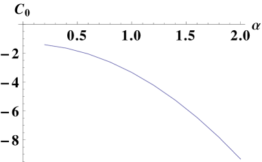
b.
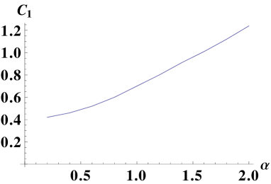
c.

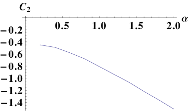
Figure 1: Variation of coefficients $C_{0},C_{1},C_{2}$ with $\alpha$

Now rescaling the variables $\tau,\xi$ and $\eta$ in (18) we get

$$i\frac{\partial n_{1}^{(1)}}{\partial_{t}}+\frac{\partial^{2}n_{1}^{(1)}}{\partial_{x}\partial_{y}}+2in_{1}^{(1)}(n_{1}^{(1)}\frac{\partial n_{1}^{(1)*}}{\partial_{x}}-n_{1}^{(1)*}\frac{\partial n_{1}^{(1)}}{\partial_{x}})=0$$ (20)

and renaming $n_{1}^{(1)}$ as $u$ it gives

$$iu_{t}+u_{xy}+2iu(uu_{x}^{*}-u^{*}u_{x})=0$$ (21)

which is our new (2+1) dimensional completely integrable evolution equation that has been obtained at a higher perturbation order compared to the NLS equation, hence expected to address weaker effects. Similar equation was derived in the context of water wavesMyRogue in order to model oceanic rogue waves. It has structural similarity with the NLS equation, where the nonlinearity comes from the ponderomotive force that depends on the square of modulus and not on the phase of $u$. The present equation(21) has slightly different characteristics, with the nonlinear potential dependent on the square of modulus of the wave profile as well as on the x-derivative of phase. The dispersive term, is a cross derivative term dependent on both longitudinal and transverse directions.

The study of propagation of modulated ion acoustic waves in the presence of a magnetic field has been extensively done using the NLS equation that restricts the study to one dimension. A multidimensional generalization of the NLS equation for a modulated ion acoustic wave packet propagating in a magnetized plasma leads to the Davey Stewartson equation Nishinari ; Annou . However, since all the spatial directions are scaled symmetrically, this equation certainly does not describe weak transverse propagation. In the long wave length regime, the KP equation is well known to describe the propagation of such waves when weak transverse perturbation is considered Dahiya ; Kako ; Mushtaq . In an effort to obtain a 2D extension with weak transverse dependence of modulated ion wave packets propagating in a magnetized plasma, we obtain an asymmetric (2+1) dimensional novel equation(21) along with a space-like NLS equation (12). Hence, we observe that our equation has resemblance to the KP equation from the point of weak transverse propagation, and to the DS equation from its modulated structure. In case of DS or KP, the system reduces to NLS or KdV equation respectively when the transverse coordinate is neglected, but the present equation given in (21) does not reduce to the standard NLS equation in such limit, indicating its distinctive asymmetric nature.

The various properties, as well as the solutions of this new equation are explored in the foregoing sections of the paper.

III Modulation instability

Instability of a planar wave, appearing due to the interplay between dispersion and nonlinear effect called modulation instability (MI) BF , which has been in the continuous focus for many years McLean ; Ramamonjiarisoa .

For investigating the contributions to the frequency due to the linear dispersive and the nonlinear term in (18), we insert the plane wave solution $q_{0}=A_{0}\ e^{i(\omega t+k^{x}x+k^{y}y)},$ with $A_{0}$ as the real constant amplitude, $\omega$ as frequency and $(k^{x},k^{y})$ as the wave vector . For the plane wave to be an exact solution of (18), the frequency should be $\omega=\omega_{L}+\omega_{NL},\ \omega_{L}=-\frac{C_{1}}{C_{0}}k^{x}k^{y},\ \omega_{NL}=\frac{2C_{2}}{C_{0}}A_{0}^{2}k^{x},$ where $\omega_{L}$ is the frequency due to linear dispersion and $\omega_{NL}$ is its nonlinear correction, which depends on the amplitude of the wave as well as on the x component of the wave vector.

Now to explore the onset of MI in the system affecting this plane wave solution, we perturb it by a small parameter function $\epsilon(x,y,t)$. Note that the perturbation is considered in both the space directions.

The solution

$$q_{\epsilon}=(A_{0}+\epsilon)e^{i(\omega t+k^{x}x+k^{y}y)}$$ (22)

neglecting the higher order terms in $\epsilon$ yields from (18) a linear equation for $\epsilon$ as

$$iC_{0}\epsilon_{t}+C_{1}\epsilon_{xy}+iC_{1}(k^{y}\epsilon_{x}+k^{x}\epsilon_{y})+iC_{2}A_{0}^{2}(\epsilon_{x}^{*}-\epsilon_{x})+2C_{2}A_{0}^{2}k^{x}(\epsilon^{*}+\epsilon)=0.$$ (23)

For detecting the instability of the perturbation we represent

$$\epsilon=k_{1}e^{i(\omega_{m}t+k^{x}_{m}x+k^{y}_{m}y)}+k_{2}e^{-i(\omega_{m}t+k^{x}_{m}x+k^{y}_{m}y)}.$$ (24)

Inserting this form of perturbation in equation (23) and arranging the independent terms we get a set of two homogeneous equations for the arbitrary coefficients $k_{1},k_{2},$ nontrivial solutions of which can exist only when the determinant of the matrix vanishes leading to the necessary relation ${\bar{\omega}_{m}}^{2}=K^{2}-{\Omega_{c}},$ where  $\bar{\omega}_{m}=C_{0}\omega_{m}-\omega_{0},$  and  $\omega_{0}=C_{2}A_{0}^{2}k_{m}^{x}-C_{1}{k^{x}}{k_{m}^{y}}-C_{1}{k_{m}^{x}}{k^{y}},$  $K=C_{1}{k_{m}^{x}}{k_{m}^{y}}-2C_{2}A_{0}^{2}k^{x},\ \ \Omega_{c}=A_{0}^{4}(4C_{2}^{2}{k^{x}}^{2}-C_{2}^{2}{k_{m}^{x}}^{2}),$ which gives finally

$$C_{0}\omega_{m}=\omega_{0}\pm i\omega_{i},\ \omega_{i}=(\Omega_{c}-K^{2})^{\frac{1}{2}}=(4C_{2}C_{1}{k_{m}^{x}}{k_{m}^{y}}k^{x}A_{0}^{2}-C_{2}^{2}A_{0}^{4}{k_{m}^{x}}^{2}-C_{1}^{2}{k_{m}^{x}}^{2}{k_{m}^{y}}^{2})^{\frac{1}{2}}.$$ (25)

Therefore, under the condition $K^{2}<{\Omega_{c}}$ which is $4C_{2}C_{1}{k_{m}^{x}}{k_{m}^{y}}k^{x}A_{0}^{2}>C_{2}^{2}A_{0}^{4}{k_{m}^{x}}^{2}+C_{1}^{2}{k_{m}^{x}}^{2}{k_{m}^{y}}^{2}$ with ${\Omega_{c}}>0$, i.e when $|{k_{m}^{x}}|<2|{k^{x}}|$ the modulation frequency $\omega_{m}$ can acquire an imaginary part $\omega_{i},$ initiating an exponential growth of perturbation with time $t$ and hence onsetting the MI. $\omega_{i}$ is the growth rate of the instability given by (25), a graphical form of which is presented in Fig. 2, showing its dependence on the longitudinal and transverse directions through $k_{x}^{m}$, and $k_{y}^{m}$ respectively. For plotting the growth rate and stability region, specific values of $C_{0},C_{1}$ and $C_{2}$ are chosen from Figure (1) as -1.65, 0.46 and -0.49 respectively when $\alpha=0.4$. Both these figures show clearly that the behavior of MI as well as growth rate has a strong directional preference and range.

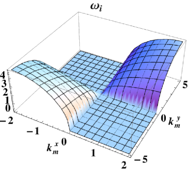
Figure 2: The growth rate $\omega_{i}$ of the MI given by (25), arising in our new equation, exhibiting how it changes (for $A_{0}=1.0,k^{x}=-5.0$) along the longitudinal $(k_{m}^{x})$ and transverse ($k_{m}^{y}$) directions, showing a strong directional preference.

The stability plot is drawn in Fig. 3 in the $(k^{x}_{m},k^{y}_{m})$ plane with the shaded region showing the domain of MI.

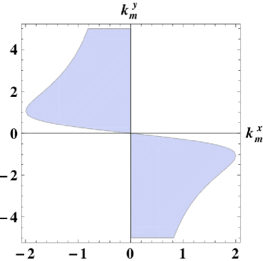
Figure 3: Graphical representation of the MI region, where the instability can occur only within the shaded area (for fixed values of $A_{0}=1.0,K^{x}=-5.0$). The instability region, showing dependence on the wave vector $(k_{x}^{m},k_{y}^{m})$, varies asymmetrically along the longitudinal and transverse direction, as seen clearly from the figure.

A comparison with these obtained conditions of MI of (21) with other modulated wave equations may be illuminating. Evolution of a wave satisfying one dimensional NLS equation depends on the product of the coefficients of nonlinear and dispersive termsMoslem , which are the functions of the physical parameters involved. If the product is positive, the amplitude modulated envelope is unstable for perturbation wavelengths larger than a critical value, hence the carrier wave may either collapse or lead to formation of bright envelope modulated wave packets. On the other hand if the product is negative, the amplitude modulated envelope will be stable against external perturbations and may propagate in the form of a dark envelope wave packet. For dust acoustic waves and dust ion acoustic waves following NLS equationAmin , amplitude modulation is considered to propagate oblique to the direction of the pump carrier wave propagation in Amin and a wide domain of angle and frequency has been found where the modulation is unstable. In case of the propagation of ion acoustic envelope solitons in cylindrical and spherical geometries following modified NLS equation in multicomponent plasma with positronsSabry , a modulation instability period has been found, which does not exist in one dimension. It is found that spherical waves are more structurally stable to perturbations than the cylindrical waves and increasing positron concentration leads to a decrease in critical wave number until the concentration reaches a critical value and then further increase of concentration leads the critical wave number to increaseSabry .

These are the discussions in (1+1) dimension following one space directions. The situation becomes more complicated and intricate if the transverse perturbations are included. For example, the propagation of dust ion acoustic waves with combined effect of bounded cylindrical geometry and transverse perturbationsXue leads to cylindrical DS equation. MI features of this system is widely different from the one dimensional case involving extended parameter domain and time dependence in instability condition.

Our system (18) is also (2+1) dimensional involving asymmetric dependence on the transverse coordinate. From the condition (25) we see that the growth rate and instability condition is more complicated involving all longitudinal and transverse components $(k^{x}_{m},k^{y}_{m})$ with a strong directional preference and range $|{k_{m}^{x}}|<2|{k^{x}}|$, compared to the one dimensional case. The conditions also involve the coefficients $C_{1},C_{2}$ of equation (18) which are the functions of the system parameters $k_{x},k_{y}$ and $\alpha$. The graphical variation of $C_{1},C_{2}$ with magnetic field $\alpha$ for given set of $k_{x},k_{y}$ is shown in Figure-1 from where we can see that numerical value of both $C_{1},C_{2}$ increases as we increase the magnetic field. Since the product $C_{1}C_{2}$ is negative, modulation instability can set in when the product $k^{x}_{m}k^{y}_{m}k^{x}$ is negative, and the system remains modulationally stable for positive values of $k^{x}_{m}k^{y}_{m}k^{x}$ . These are the interesting features of our exact model having distinct structure than the (1+1) dimensional NLS or (2+1) dimensional DS equation.

IV Connection with Kadomtsev- Petviashvili (KP) equation

It is interesting to note that the new integrable equation (21) together with the space NLS equation derived in (12), has a deep connection with another wellknown (2+1) dimensional evolution equation. The equation (21) along with (12) is a complex equation denoting ion acoustic wave with modulation. But if we are concerned with the modulus of the wave, then our system also provides another well known, integrable equation.

Equation (21) is our new evolution equation after scaling, while the space NLS equation (12) at the same scaling becomes

$$iu_{y}=Bu_{xx}+A|u^{2}|u,$$ (26)

where $A,B$ are two real constants dependent on $C_{1},C_{2}$ as $B=-\frac{B_{1}^{(3)}C_{2}}{A_{1}^{(3)}C_{1}}$, $A=-\frac{C_{1}^{(3)}C_{1}}{A_{1}^{(3)}C_{2}}$. Now, if (21) is multiplied by $u$ and its complex conjugate equation by $u^{*}$ and subtracted from one another, then taking derivative w.r.t $x$ we get another equation containing quadratic power in $u$. Now using (26) and its complex conjugate equation, that equation can be simplified to yield

$$[4B\phi_{t}-6AB\phi\phi_{x}-B^{2}\phi_{xxx}]_{x}+3\phi_{yy}=0,$$ (27)

where $\phi=uu^{*}$.

Equation (27) is nothing but the well known KP equation where $\phi$ being the square of modulus of the wave $u$, the dependent variable of equations (21) and (26). It means that the square of the absolute value of the wave without modulation satisfies another real equation which is also integrable and weak in the transverse perturbation. Note that, in the derivation of (21) we have implied weak scaling on the transverse coordinate, similar as the scaling involved in the derivation of KP equation. Hence our equation (21) though being a modulated equation in two dimensions, has a different structure than the DS equation which is symmetric in both the spatial variables and has a connection with another two dimensional long wave equation which is asymmetric in the transverse direction.

For ion acoustic wave, KP equation has been derived and its stability properties under transverse perturbations have been discussed in many plasma systems like quantum electron ion plasmaMushtaq or in electron-positron-ion plasma with high energy tail electron and positron distributionShahmansouri and in other fields and using Sagdev potential approach conditions of existance of stable solitary waves have been obtained. Unlike KdV equation where the form of soliton solution does not depend on the sign of the dispersion term, the form of soliton solution of KP equation is directly determined by the dispersion sign. Again the stability of the soliton depends on the coefficients of the KP equation which in this case also depends on the coefficients of (18) and (12). Depending on the signs of $A,B$ equation (27) can be transformed into KP-I or KP-II equations admitting different types of solutions . The square root of various solutions of (27) can be used for constructing the solution of (21) together with a phase factor connected with (26), which we plan to explore in the future. The connection of our equation (21) with KP equation stresses the two dimensional and asymmetric nature of the equation.

V Soliton solutions

As a direct feature of integrable system, our equation, (21) must admit higher soliton solutions. In this section we will elaborately discuss its multisoliton solutions, which can be derived by many methods e.g, inverse scattering transform, Hirota method and various dressing methods. The IST method is more powerful (it can handle general, initial conditions) and at the same time more complicated. But, if one just wants to find soliton solutions, Hirota’s method is fastest in producing results Hirota ; Lakshmanan . Hence, following the method, we use the bilinearizing transformation given by

$$u(x,y,t)=\frac{G(x,y,t)}{F(x,y,t)},$$ (28)

where $G(x,y,t)$ and $F(x,y,t)$ are complex and real functions respectively. Using (21) one derives a pair of bilinear equations:

$$i(FG_{t}-GF_{t})+(FG_{xy}+GF_{xy}-G_{x}F_{y}-G_{y}F_{x})=0,2i(GG_{x}^{*}-G^{*}G_{x})+2(F_{x}F_{y}-FF_{xy})=0.$$ (29)

Multisoliton solutions are obtained by finite perturbation expansions as

$$F=1+\epsilon^{2}F_{2}+\epsilon^{4}F_{4}+\cdots,G=\epsilon G_{1}+\epsilon^{3}G_{3}+\cdots,$$ (30)

where $\epsilon$ is formal expansion parameter need not to be small. Collecting like powers of $\epsilon$, we obtain the following series of equations:

$${\rm O}(\epsilon):\ \ iG_{1t}+G_{1xy}=0$$ (31)

$${\rm O}(\epsilon^{2}):\ \ 2F_{2xy}=2i[G_{1}G_{1x}^{*}-G_{1}^{*}G_{1x}]$$ (32)

$${\rm O}(\epsilon^{3}):\ \ iG_{3t}+G_{3xy}=i[G_{1}F_{2t}-F_{2}G_{1t}]-[F_{2}G_{1xy}+G_{1}F_{2xy}-G_{1x}F_{2y}-G_{1y}F_{2x}]=0$$ (33)

$${\rm O}(\epsilon^{4}):\ \ 2F_{4xy}=2i[G_{3}G_{1x}^{*}+G_{1}G_{3x}^{*}-G_{3}^{*}G_{1x}-G_{1}^{*}G_{3x}]+2[F_{2x}F_{2y}-F_{2}F_{2xy}]$$ (34)

and similarly higher order equations.

V.1 1-soliton

To construct 1-soliton solution for (21) we assume the ansatz

$$G_{1}=e^{\eta_{1}},\ \eta_{1}=k_{1}x+p_{1}y-w_{1}t+\eta_{1}^{0}$$ (35)

where $k_{1},p_{1},w_{1},\eta_{1}^{0}$ are complex constants. From equation (31) therefore one obtains the associated dispersion relation $\ w_{1}=-ik_{1}p_{1},\$ using which the equation (32) is solved easily to yield

$$F_{2}=i(k_{1}^{*}-k_{1})\frac{e^{(\eta_{1}+\eta_{1}^{*})}}{(p_{1}+p_{1}^{*})(k_{1}+k_{1}^{*})}.$$ (36)

We can verify using (35) and (36), that all higher order terms in $\epsilon$ beyond $G_{1}$ and $F_{2}$ trivially vanish. Absorbing $\epsilon$ in arbitrary constant $\eta_{1}^{0}$, we construct from (28) using (35) and (36) the 1 soliton solution in the form

$$u(x,y,t)=\frac{G_{1}}{1+F_{2}}=\frac{e^{\eta_{1}}}{1+\alpha e^{(\eta_{1}+\eta_{1}^{*})}}$$ (37)

where $\alpha$ depends on the parameter $k_{1},p_{1}.$ One can identify the interesting 2d nature of our equation (21) by making $p_{1}=0$, then from eq. (36) we can see that $F_{2}$ will diverge and no soliton solution can be found. If additionally we use the dispersion relation of the constraint equation

$$iu_{y}+u_{xx}+2|u|^{2}u=0$$ (38)

which comes from (12), as $p_{1}=-ik_{1}^{2}$, the soliton solution (37) simplifies to yield the conventional form

$$q(x,y,t)={\rm sech}\xi\ e^{i\theta},\ \mbox{with}\ \xi=\eta(x+v_{y}y+vt),\ \theta=(k_{x}x+k_{y}y+\omega t).$$ (39)

A frozen picture of the modulus of our travelling soliton solution (39) at time $t=0$ is shown in Fig. 4.

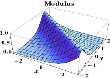
Figure 4: Modulus of 1 soliton with $k_{1r}=1,k_{1i}=1,\eta_{1r}^{0}=1,\eta_{1i}^{0}=-1$ and at t=0

V.2 2-Soliton

For obtaining 2-soliton solution we start with the standard procedure assuming

$$G_{1}=e^{\eta_{1}}+e^{\eta_{2}},\eta_{1}=k_{1}x+p_{1}y-w_{1}t+\eta_{1}^{0},\ \eta_{2}=k_{2}x+p_{2}y-w_{2}t+\eta_{2}^{0},$$ (40)

where the parameters involved are complex numbers. Applying similar dispersion relations as earlier we get $w_{1}=-ik_{1}p_{1},\ w_{2}=-ik_{2}p_{2}$ and obtain from (32)

$${F_{2}=[e^{(\eta_{1}+\eta_{1}^{*}+R_{1})}+e^{(\eta_{2}+\eta_{2}^{*}+R_{2})}}+e^{(\eta_{2}+\eta_{1}^{*}+\delta_{0})}+{e^{(\eta_{1}+\eta_{2}^{*}+\delta_{0}^{*})}]},$$ (41)

where all the constant parameters can be worked out explicitly (see Appendix ). Similarly equation (33) at higher order expansion gives

$${G_{3}=e^{(\eta_{1}+\eta_{1}^{*}+\eta_{2}+\delta_{1})}+e^{(\eta_{1}+\eta_{2}^{*}+\eta_{2}+\delta_{2})}},$$ (42)

where the relevant parameter details are given in Appendix . Using further equation (34) one obtains

$$F_{4}=e^{(\eta_{1}+\eta_{1}^{*}+\eta_{2}+\eta_{2}^{*}+R_{3})},$$ (43)

with the relevant parameters presented in Appendix. For simplifying the expressions,as mentioned earlier, we can use the constraint equation (38), imposing the relations between $k_{1}$ , $p_{1}$ and $k_{2}$ , $p_{2}$ as $p_{1}=-ik_{1}^{2}$ , $p_{2}=-ik_{2}^{2}$ (see Appendix). Here we find again, that the higher order terms in $\epsilon$ beyond $G_{3}$ and $F_{4}$ trivially vanish, leaving the exact 2- soliton solution in the form

$$u(x,y,t)=\frac{G_{1}+G_{3}}{1+F_{2}+F_{4}}$$ (44)

Here also we can see that for no transverse dependence i.e. $p_{1}=p_{2}=0$, all the quantities determined $F_{2},G_{3},F_{4}$ diverges and two soliton solution cannot be found which indicates the strict 2d nature of the equation. A graphical plot of the modulus of this solution in $(2+1)$-dimensions, frozen at time $t=2$, is shown in Fig. 5, where the 2-soliton as two interacting 1-solitons is clearly seen on a 2D $(x,y)$-plane. Following the same procedure the higher soliton solutions of our equation can be evaluated.

These one and two soliton solutions of (21) have similarities with the soliton solutions of NLS equation with an additional transverse dependence. Since a purely 1D model cannot account for the observed features of many physical situations, specially in auroral region with higher polar altitudesFranz corresponding 2D model is necessary. There lies the importance of the soliton solutions of our equation (21), which could be applied to many research areas of this field.

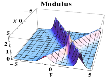
Figure 5: Modulus of 2 soliton with $k_{1r}=1,k_{1i}=1,k_{2r}=2,k_{2i}=-1,\eta_{1r}^{0}=1,\eta_{1i}^{0}=1,\eta_{2r}^{0}=1,\eta_{2i}^{0}=1$ and at t=2

VI Exact static 2D lump solution:

Localized wave structure in (2+1) dimensional systems are very important in terms theoretical and experimental aspects of plasma. Localized rational structure following KP-I equation have been found by Janaki et.al in the propagation of oblique magnetosonic wave in warm collisional plasma systemJanaki , where the wave profile decays algebraically in both directions. Whereas, in case of modulated wave equation like Davey Stewartson system, an exponentially localized solution called Dromion, which moves with time has been found in magnetized electron acoustic wave system Ghosh . Our equation (21) which has some similarity with both DS and KP equations, also possesses an exact localized wave solution, decaying rationally in both spatial directions.

The static 2D rational lump solution is given by

$$u_{static}(x,y)=exp(4iy)(\frac{1-4iy}{c+\alpha_{1}x^{2}+4y^{2}}-1)$$ (45)

where c , $\alpha_{1}$ are 2 free parameters. From this we can see that the wave attains the maximum amplitude

$$A_{max}=\frac{1-c}{c}$$ (46)

at the centre x=0, y=0 which can be controlled by c. At large distances($|x|$ $\rightarrow\infty$,$|y|$ $\rightarrow\infty$) the amplitude goes to unity. The steepness of this static wave solution as observed from the front is $\frac{\partial}{\partial y}{u_{static}}$ is related to another free parameter $\alpha_{1}$.The amplitude of the wave falls to its minimum at x=0, $y=\pm y_{0}$, with $y_{0}=\sqrt{\frac{1-c}{\alpha_{1}}}$. Hence the density gets localized at the centre x=0,y=0 and the concentration can be controlled by the free parameter $c$. This is an interesting feature because in actual physical situation the ion density can change which need to be controlled by the free parameters. This is absent in the (1+1) dimensional NLS system, where Peregrine breather which is used to describe density localization in the x-t plane, have no free parameters and hence can achieve a fixed maximum value (3 times than the background). Whereas our solution, having two free parameters $c$ and $\alpha_{1}$ can achieve any amplitude and steepness, relevant to the actual physical condition.

Thus unlike the exponentially decaying dromion solution of DS1 equation, our system (21) provides a rational solution in both space directions having similar structure to the rational solution of KP-I equation. There lies another connection of the equation (21) with KP which has similar scaling and weaker dependence on transverse directions as (21). Unfortunately, the time evolution of the rational solution (45) could not be found which can be explored in future.

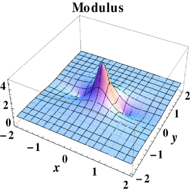
Figure 6: Absolute value of the solution (45) with c=1/6, $\alpha=6/5$

VII Other integrable properties: Lax Pair, Conserved quantities

Since our new equation (21) is a completely integrable system, it possesses the associated integrable properties. One of such properties i.e, existence of higher soliton solutions, have been discussed using Hirota bilinearization method in the previous section. We briefly state here the other properties such that existence of Lax pairs, infinite number of conserved quantities etc mypaper .

For equation (21), one can find the associated linear system $\Phi_{y}=U(\lambda)\Phi,\Phi_{t}=V(\lambda)\Phi,$ with a Lax pair given by

$$U(\lambda)\equiv V_{2}(\lambda)=2\lambda V_{1}(\lambda)+V_{2}^{(0)},\ V(\lambda)\equiv V_{3}(\lambda)=2\lambda V_{2}(\lambda)+V_{3}^{(0)}$$ (47)

where

$$V_{1}(\lambda)=i(\lambda\sigma^{3}+U^{(0)}),\ V_{2}^{(0)}=\sigma^{3}(U^{(0)}_{x}-i{U^{(0)}}^{2})$$

$$V_{3}^{(0)}=-\sigma^{3}U^{(0)}_{y}-[U^{(0)},U^{(0)}_{x}],\ U^{(0)}=q\sigma^{+}+q^{*}\sigma^{-},$$ (48)

with $\sigma^{a},a=\pm,3,$ Pauli matrices. The flatness condition: $U_{t}-V_{y}+[U,V]=0$, of the given Lax Pair gives our equation (21) together with the space NLS equation like (26) for particular values of $A$ and $B$. The derivation done in sec II from the two fluid equations for a magnetized plasma has shown to lead to the space NLS as well as the 2d evolution equation(21) at different orders of perturbation, which is consistent with the Lax pair formalism.

Systems with infinite degrees of freedom like (21), when integrable, should have infinite set of independent conserved quantities, which can be derived explicitly as

$$C_{1}=i\int dy(q^{*}q_{x}-q^{*}_{x}q),\ C_{2}=\int dy(i\frac{1}{2}(q^{*}_{y}q-q^{*}q_{y})+q^{*}_{x}q_{x}+|q|^{4}),\ C_{3}=\int dy(q^{*}_{y}q_{x}+q^{*}_{x}q_{y}),$$

$$C_{4}=\int dy\left(iq^{*}_{xy}q_{x}+q^{*}_{y}q_{y}-i|q|^{2}(q^{*}q_{y}-q^{*}_{y}q)-2|q|^{2}\ q^{*}_{x}q_{x}+({q^{*}}^{2}q^{2}_{x}+{q_{x}^{*}}^{2}q^{2})\right),$$ (49)

and so on. Note the involvement of both the space-variables $x,y$ in this series of independent conserved quantities, which also gives another argument in favor of the integrability of the 2D nonlinear equation (21). Nevertheless, the one dimensional integral of these conserved quantities signifies also about,a quasi-2D nature of this system.

VIII Conclusive remarks

In this work a completely integrable, (2+1) dimensional, modulated , nonlinear evolution equation has been derived in the ion acoustic wave of magnetized collisionless plasma system. It has been obtained at a higher perturbation order compared to the NLS equation, hence expected to address weaker effects. The two spatial directions are scaled asymmetrically allowing weak transverse perturbation. Thus the equation derived (21), has connection with the DS equation in terms of its modulated structure, with KP equation in terms of its weak transverse dependence. Condition of modulation instability and nonlinear frequency shift clearly shows the spatial asymmetry in growth rate, which is a distinct feature compared to the one dimensional case. Dependence of the onset condition of MI with magnetic field and other system parameters are discussed. It is shown that the square of modulus of the dependent variable of the equation satisfies KP equation along with the space NLS like constraint(12) equation. Its Lax Pair structure is discussed and infinite conserved quantities are derived briefly. Using Hirota bilinearization scheme its higher soliton solutions are calculated which has similar structure with the 1D soliton with an additional dependence on transverse direction. The exact algebraic lump solution of (21), carrying 2 free parameters is also given and density localization of the system is discussed. Applications of this important and novel equation in various aspects of plasmas and identification of its different features may pave a new direction of research in this field.

IX Appendix:

i) Coefficients appearing in the derivation of the two dimensional integrable evolution equation (21), given in section-II:

$K_{1}=\frac{1}{1+|k|^{2}}$, $|k|^{2}=(k_{x}^{2}+k_{y}^{2})$,$\kappa_{1}=\frac{1}{1+4|k|^{2}}$, $A_{1}^{(1)}=-\frac{(iK_{1}k_{y}\alpha+K_{1}k_{x}\omega)}{(\alpha^{2}-\omega^{2})}$, $B_{1}^{(1)}=\frac{(iK_{1}k_{x}\alpha-K_{1}k_{y}\omega)}{(\alpha^{2}-\omega^{2})}$

$A_{0}^{(2)}=\frac{-2\omega k_{x}}{|k|^{2}}$, $B_{0}^{(2)}=\frac{-2\omega k_{y}}{|k|^{2}}$,

$A_{1}^{(2)}=-\frac{(iK_{1}k_{y}\alpha+K_{1}k_{x}\omega)}{(\alpha^{2}-\omega^{2})}$, $C_{1}^{(2)}=-\frac{(-iK_{1}k_{x}\alpha^{3}+K_{1}k_{y}\alpha^{2}\omega+iK_{1}k_{x}\alpha\omega^{2}-K_{1}k_{y}\omega^{3})}{(-\alpha^{2}+\omega^{2})^{2}}$,

$D_{1}^{(2)}=-\frac{(-iK_{1}k_{y}M_{x}\alpha^{2}-K_{1}\alpha^{3}+2K_{1}^{2}k_{x}^{2}\alpha^{3}-2K_{1}k_{x}M_{x}\alpha\omega+2iK_{1}^{2}k_{x}k_{y}\alpha^{2}\omega-iK_{1}k_{y}M_{x}\omega^{2}+K_{1}\alpha\omega^{2}-2K_{1}^{2}k_{x}^{2}\alpha\omega^{2}-2iK_{1}^{2}k_{x}k_{y}\omega^{3})}{(-\alpha^{2}+\omega^{2})^{2}}$,

$B_{1}^{(2)}=-\frac{\{-2K_{1}^{2}k_{x}k_{y}\alpha-iK_{1}\omega+2iK_{1}^{2}k_{x}^{2}\omega-(iK_{1}k_{x}M_{x}\alpha^{2})/(\alpha^{2}-\omega^{2})+(2K_{1}k_{y}M_{x}\alpha\omega)/(\alpha^{2}-\omega^{2})-(iK_{1}k_{x}M_{x}\omega^{2})/(\alpha^{2}-\omega^{2})\}}{(\alpha^{2}-\omega^{2})}$,

$A_{2}^{(2)}=\{-2K_{1}^{3}k_{x}|k|^{4}\kappa_{1}+K_{1}|k|^{2}(5k_{x}\alpha^{2}+3ik_{y}\alpha\omega+4k_{x}^{3}\kappa_{1}+\\ 4k_{x}k_{y}^{2}\kappa_{1})+\alpha^{2}(3k_{x}\alpha^{2}+3ik_{y}\alpha\omega+4k_{x}|k|^{2}\kappa_{1})+K_{1}^{2}|k|^{2}(2k_{x}|k|^{2}-2k_{x}\alpha^{2}\kappa_{1}-ik_{y}\alpha\omega\kappa_{1})\}/\{3\alpha^{2}\omega|k|^{2}+4|k|^{4}\omega(K_{1}-\kappa_{1})\}$,

$B_{2}^{(2)}=\{-2K_{1}^{3}k_{y}|k|^{2}\kappa_{1}+K_{1}|k|^{2}(5k_{y}\alpha^{2}-3ik_{x}\alpha\omega+\\ 4k_{x}^{2}k_{y}\kappa_{1}+4k_{y}^{3}\kappa_{1})+\alpha^{2}(3k_{y}\alpha^{2}-3ik_{x}\alpha\omega+4k_{y}|k|^{2}\kappa_{1})+K_{1}^{2}|k|^{2}(2k_{y}|k|^{2}-2k_{y}\alpha^{2}\kappa_{1}+ik_{x}\alpha\omega)\}/\{3\alpha^{2}\omega|k|^{2}+4|k|^{4}\omega(K_{1}-\kappa_{1})\}$,

$C_{2}^{(2)}=2\frac{\{3\alpha^{2}+K_{1}|k|^{2}(3-K_{1}\kappa_{1})\}}{\{3\alpha^{2}+4|k|^{2}(K_{1}-\kappa_{1})\}}$,

$D_{2}^{(2)}=\frac{\{-4K_{1}(-3+K_{1}^{2})|k|^{2}-3(-4+K_{1}^{2})\alpha^{2}\}\kappa_{1}}{\{6\alpha^{2}+8|k|^{2}(K_{1}-\kappa_{1})\}}$,

$A_{1}^{(3)}=2K_{1}k_{y}\omega(|k|^{2}K_{1}-1)$,

$B_{1}^{(3)}=\frac{-K_{1}(K_{1}|k|^{2}-1)\{K_{1}(-k_{y}^{2}+3K_{1}k_{x}^{2}|k|^{2})+(4K_{1}k_{x}^{2}-1)\alpha^{2}\}}{\omega}$,

$C_{1}^{(3)}=|k|^{2}\omega[K_{1}\{4K_{1}(K_{1}^{3}-3)|k|^{2}+3(K_{1}^{3}-4)\alpha^{2}\}+\{4K_{1}(12+K_{1}^{2}(K_{1}-3)(K_{1}+2)\}|k|^{2}+3(k_{1}^{2}-4)^{2}\alpha^{2}\}\kappa_{1}]/\{6\alpha^{2}+8|k|^{2}(K_{1}-\kappa_{1})\}$,

$A_{0}^{(3)}=-\frac{1}{\alpha}[A_{1}^{(1)*}B_{1}^{(1)}-iB_{1}^{(2)}B_{1}^{(1)*}k_{x}+iA_{1}^{(1)*}D_{1}^{(2)}k_{x}-B_{0}^{(2)}M_{x}]$

$B_{0}^{(3)}=-\frac{1}{\alpha}[A_{1}^{(1)}B_{1}^{(1)*}-iB_{1}^{(1)}B_{1}^{(2)*}k_{x}-iA_{1}^{(1)}D_{1}^{(2)*}k_{x}-B_{0}^{(2)}M_{x}]$

$C_{0}^{(3)}=\frac{i}{\alpha}[A_{1}^{(2)}B_{1}^{(1)*}-A_{1}^{(1)*}C_{1}^{(2)}]k_{x}$

$D_{0}^{(3)}=-\frac{i}{\alpha}[A_{1}^{(2)*}B_{1}^{(1)}-A_{1}^{(1)}C_{1}^{(2)*}]k_{x}$

$E_{0}^{(3)}=\frac{1}{\alpha}[A_{1}^{(1)}A_{1}^{(1)*}-K_{1}^{2}+iB_{1}^{(2)}B_{1}^{(1)*}k_{y}-iA_{1}^{(1)*}D_{1}^{(2)}k_{y}-A_{0}^{(2)}M_{x}]$

$F_{0}^{(3)}=\frac{1}{\alpha}[A_{1}^{(1)}A_{1}^{(1)*}-K_{1}^{2}-iB_{1}^{(1)}B_{1}^{(2)*}k_{y}+iA_{1}^{(1)}D_{1}^{(2)*}k_{y}-A_{0}^{(2)}M_{x}]$

$G_{0}^{(3)}=\frac{i}{\alpha}[A_{1}^{(2)}B_{1}^{(1)*}-A_{1}^{(1)*}C_{1}^{(2)}]k_{y}$

$H_{0}^{(3)}=-\frac{i}{\alpha}[A_{1}^{(2)*}B_{1}^{(1)}-A_{1}^{(1)}C_{1}^{(2)*}]k_{y}$

$L_{0}^{(3)}=\frac{1}{M_{x}\alpha}[A_{1}^{(1)}\alpha+A_{1}^{(2)*}\alpha+iA_{1}^{(1)}C_{1}^{(2)*}k_{x}-iA_{1}^{(2)*}B_{1}^{(1)}k_{x}]$

$K_{0}^{(3)}=\frac{1}{M_{x}\alpha}[A_{1}^{(2)}\alpha+A_{1}^{(1)*}\alpha+iA_{1}^{(2)}B_{1}^{(1)*}k_{x}-iA_{1}^{(1)*}C_{1}^{(2)}k_{x}]$

$J_{0}^{(3)}=\frac{1}{M_{x}\alpha}[-A_{1}^{(1)}B_{1}^{(1)*}-iB_{1}^{(1)}B_{1}^{(2)*}k_{x}+iA_{1}^{(1)}D_{1}^{(2)*}k_{x}+B_{0}^{(2)}M_{x}+B_{1}^{(2)*}\alpha]$

$I_{0}^{(3)}=\frac{1}{M_{x}\alpha}[-B_{1}^{(1)}A_{1}^{(1)*}+iB_{1}^{(1)*}B_{1}^{(2)}k_{x}-iA_{1}^{(1)*}D_{1}^{(2)}k_{x}+B_{0}^{(2)}M_{x}+B_{1}^{(2)}\alpha]$

$Q_{0}^{(3)}=-\frac{1}{M_{x}\alpha}[iA_{1}^{(2)*}B_{1}^{(1)}k_{x}-iA_{1}^{(1)}C_{1}^{(2)*}k_{x}-A_{1}^{(1)}\alpha-A_{1}^{(2)*}\alpha+K_{1}^{2}M_{x}\alpha]$

$P_{0}^{(3)}=\frac{1}{M_{x}\alpha}[-A_{1}^{(1)}B_{1}^{(1)*}-iB_{1}^{(1)}B_{1}^{(2)*}k_{x}+iA_{1}^{(1)}D_{1}^{(2)*}k_{x}+B_{0}^{(2)}M_{x}+B_{1}^{(2)*}\alpha+2iK_{1}^{3}k_{x}M_{x}\alpha]$

$M_{0}^{(3)}=\frac{1}{M_{x}\alpha}[-A_{1}^{(1)*}B_{1}^{(1)}-iB_{1}^{(2)}B_{1}^{(1)*}k_{x}-iA_{1}^{(1)*}D_{1}^{(2)}k_{x}+B_{0}^{(2)}M_{x}+B_{1}^{(2)}\alpha-2iK_{1}^{3}k_{x}M_{x}\alpha]$

$N_{0}^{(3)}=-\frac{1}{M_{x}\alpha}[-iA_{1}^{(2)}B_{1}^{(1)*}k_{x}+iA_{1}^{(1)*}C_{1}^{(2)}k_{x}-A_{1}^{(2)}\alpha-A_{1}^{(1)*}\alpha+K_{1}^{2}M_{x}\alpha]$

ii) Coefficients appearing in the Hirota bilinearization procedure in solving equation (21), given in section-V:

$$e^{R_{1}}=i\frac{(k_{1}^{*}-k_{1})}{(p_{1}+p_{1}^{*})(k_{1}+k_{1}^{*})},e^{R_{2}}=i\frac{(k_{2}^{*}-k_{2})}{(p_{2}+p_{2}^{*})(k_{2}+k_{2}^{*})},$$

$$e^{\delta_{0}}=i\frac{(k_{1}^{*}-k_{2})}{(p_{2}+p_{1}^{*})(k_{2}+k_{1}^{*})},e^{\delta_{0}^{*}}=i\frac{(k_{2}^{*}-k_{1})}{(p_{1}+p_{2}^{*})(k_{1}+k_{2}^{*})}$$

$$e^{\delta_{1}} = \frac{i}{[(k_{2}+k_{1}^{*})(p_{1}+p_{1}^{*})+(k_{1}+k_{1}^{*})(p_{2}+p_{1}^{*})]}[\frac{(k_{1}^{*}-k_{1})(p_{2}-p_{1})}{(p_{1}+p_{1}^{*})}+$$ (50)

$$+ \frac{(k_{1}^{*}-k_{1})(k_{2}-k_{1})}{(k_{1}+k_{1}^{*})}+\frac{(k_{1}^{*}-k_{2})(p_{1}-p_{2})}{(p_{2}+p_{1}^{*})}+\frac{(k_{1}^{*}-k_{2})(k_{1}-k_{2})}{(k_{2}+k_{1}^{*})}]$$

$$e^{\delta_{2}} = \frac{i}{[(k_{1}+k_{2}^{*})(p_{2}+p_{2}^{*})+(k_{2}+k_{2}^{*})(p_{1}+p_{2}^{*})]}[\frac{(k_{2}^{*}-k_{2})(p_{1}-p_{2})}{(p_{2}+p_{2}^{*})}+$$ (51)

$$+ \frac{(k_{2}^{*}-k_{2})(k_{1}-k_{2})}{(k_{2}+k_{2}^{*})}+\frac{(k_{2}^{*}-k_{1})(p_{2}-p_{1})}{(p_{1}+p_{2}^{*})}+\frac{(k_{2}^{*}-k_{1})(k_{2}-k_{1})}{(k_{1}+k_{2}^{*})}]$$

$$e^{R_{3}} = \frac{1}{(k_{1}+k_{1}^{*}+k_{2}+k_{2}^{*})(p_{1}+p_{1}^{*}+p_{2}+p_{2}^{*})}[\{ie^{\delta_{2}}(k_{1}^{*}-k_{1}-k_{2}-k_{2}^{*})$$ (52)

$$+ ie^{\delta_{1}}(k_{2}^{*}-k_{1}-k_{2}-k_{1}^{*})+ie^{\delta_{1}^{*}}(k_{1}^{*}+k_{2}^{*}+k_{1}-k_{2})+ie^{\delta_{2}^{*}}(k_{1}^{*}+k_{2}^{*}+k_{2}-k_{1})\}$$

$$+ \{(k_{2}+k_{2}^{*}-k_{1}-k_{1}^{*})(p_{1}+p_{1}^{*})+(k_{1}+k_{1}^{*}-k_{2}-k_{2}^{*})(p_{2}+p_{2}^{*})\}e^{R_{1}+R_{2}}$$

$$+ \{(k_{2}+k_{1}^{*}-k_{1}-k_{2}^{*})(p_{1}+p_{2}^{*})+(k_{1}+k_{2}^{*}-k_{2}-k_{1}^{*})(p_{2}+p_{1}^{*})\}e^{\delta_{0}+\delta_{0}^{*}}]$$

For simplifying the expressions we can impose the relations between $k_{1}$ , $p_{1}$ and $k_{2}$ , $p_{2}$ as $p_{1}=-ik_{1}^{2}$ , $p_{2}=-ik_{2}^{2}$, which would yield

$$e^{R_{1}}=\frac{1}{(k_{1}+k_{1}^{*})^{2}},e^{R_{2}}=\frac{1}{(k_{2}+k_{2}^{*})^{2}},e^{\delta_{0}}=\frac{1}{(k_{1}+k_{2}^{*})^{2}},e^{\delta_{0}^{*}}=\frac{1}{(k_{2}+k_{1}^{*})^{2}},$$

$$e^{\delta_{1}}=\frac{(k_{1}-k_{2})^{2}}{(k_{1}+k_{1}^{*})^{2}(k_{2}+k_{1}^{*})^{2}},e^{\delta_{2}}=\frac{(k_{2}-k_{1})^{2}}{(k_{2}+k_{2}^{*})^{2}(k_{1}+k_{2}^{*})^{2}},$$

$$e^{R_{3}}=\frac{|(k_{1}-k_{2})|^{4}}{(k_{1}+k_{1}^{*})^{2}(k_{2}+k_{2}^{*})^{2}(|(k_{1}+k_{2}^{*}|)^{4}}$$

References

- (1) F.F Chen Introduction to Plasma physics and controlled fusion , (Plenum Press, New York and London, 1984).
- (2) M. Lakshmanan and S. Rajasekar Nonlinear dynamics: Integrability, Chaos and Patterns, (Springer, Berlin, 2003).
- (3) H. Washimi and T. Taniuti, Phys. Rev. Lett 17, 19 (1966).
- (4) M. Q. Tran, Phys. Scr. 20, 317 (1979)
- (5) H. Ikezi, R Taylor and D. Bekar Phys. Rev. Lett 25,11 (1970).
- (6) S.E Cousens et. al, Phys. Rev. E 86, 066404 (2012).
- (7) A.A Mamun, Phys. Rev. E 77, 026406 (2008).
- (8) M. Bacha, M.Tribeche and P.K.Shukla, Phys. Rev. E 85, 056413 (2012).
- (9) S. Ghosh and N. Chakrabarti, Phys. Rev. E 84, 046601 (2011).
- (10) H. K. Malik, Phys. Rev. E 54, 5 (1996).
- (11) F. Verheest, M.A Hellberg and W.A Hereman, Phys. Rev. E 86, 036402 (2012).
- (12) P.K Shukla, A.A Mamun and D.A Mendis, Phys. Rev. E 84, 026605 (2011).
- (13) G. Huang and M.G. Velarde, Phys. Rev. E 53, 3 (1996).
- (14) S. Maxon and J. Vicelli, Phys. Fluids 17, 1614 (1974).
- (15) L.F.J Broer and F.W. Sluijter, Phys. Fluids 20, 1458 (1977).
- (16) M.R Amin, G.E Morfill and P.K Shukla, Phys. Rev. E 58, 5 (1998).
- (17) W.M Moslem, R. Sabry, S.K El-Labany and P.K Shukla, Phys. Rev. E 84, 066402 (2011).
- (18) R Sabry, W.M Moslem, P.K Shukla and H. Saleem , Phys. Rev. E 79, 056402 (2009).
- (19) W.M Moslem, Phys. Plasmas 18, 032301 (2011).
- (20) R. Sabry, W.M Moslem and P.K Shukla Phys. Rev. E 86, 036408 (2012).
- (21) N.S Javan and F. Adili, Phys. Rev. E 88, 043102 (2013).
- (22) H. Bailung, S.K Sharma and Y. Nakamura, Phys. Rev. Lett 107, 255005 (2011).
- (23) J.R Franz, P.M Kintner and J.S Pickett Geophys. Res. Lett 25, 2041 (1998).
- (24) B.B Kadomtsev and V.I Petvias‘hvili, Sov. Phys. 15, 539 (1970).
- (25) H.K. Malik and R.P. Dahiya, Phys. Lett. A 195, 369 (1994).
- (26) A. Mushtaq and S.A. Khan Phys. Plasma 14, 052307 (2007).
- (27) M. Shahmansouri and E. Astaraki J Theor. Appl. Phys 8, 189 (2014).
- (28) M. Kako and G. Rowlands, Plasma. Phys. 18, 165 (1976).
- (29) V.E Zakharov and E.A Kuznetsov Zh. Eksp. Teor. Fiz 66, 594 (1974).
- (30) V.E Zakharov and E.A Kuznetsov Sov. Phys. 39, 285 (1974).
- (31) B.K Shivamoggi, Phys. Scripta 42,641 (1990).
- (32) E Infeld and P Fryczs , J. Plasma. Phys. 37, 97 (1987).
- (33) E Infeld J. Plasma Phys. 33, 171 (1985).
- (34) B.K Shivamoggi , J. Plasma Phys. 41, 83 (1989).
- (35) A.S Bains, M Tribeche, N.S Saini and T.S Gill Phys. Plasmas 18, 104503 (2011).
- (36) S.K El-Labany, W.F.El- Tribany and O.M El-Abbasy , Phys. Plasmas 12, 092304 (2005).
- (37) N.S Saini, B.S Chahal, A.S Bains and C.Bedi Phys. Plasmas 21, 022114 (2014).
- (38) H.L Zhen, B Tian, Y.F.Wang, H.Zhong and W.R Sun Phys. Plasmas 21, 012304 (2014).
- (39) A.M Wazwaz, Comm. Non. Sc. Num. Sim 10, 597 (2005).
- (40) R.L Mace and M. A Hellberg, Phys. Plasmas 8, 2649 (2001).
- (41) K. Nishinari, K. Abe and J. Satsuma, Phys. Plasmas 1, 2559 (1994).
- (42) S.S Ghosh, A Sen and G.S Lakhina Non. Processes. Geophys 9, 463 (2002).
- (43) K. Annou and R. Annou, Phys. Plasmas 19, 043705 (2012).
- (44) J.K Xue Phys. Plasmas 12, 092107 (2005).
- (45) K Nishinari and T. Yajima, Phys. Rev. E 51, 5 (1995).
- (46) M Boiti, J.J.P Leon, L Martina and F. Pempinelli Phys. Lett. A 132 (1988).
- (47) A Kundu, A Mukherjee and T Naskar Proc. R. Soc. A 470, 20130576 (2014).
- (48) T.B Benjamin and J.E Feir J. Fluid. Mech 27, 417 (1967).
- (49) J.W McLean J. Fluid. Mech 114, 331 (1982).
- (50) C Kharif and A Ramamonjiarisoa Phys. Fluids 31, 1286 (1988).
- (51) R Hirota Phys.Rev. Lett 27, 1192 (1971)
- (52) M.S Janaki, B.K Som, B. Dasgupta and M.R. Gupta J.Phys.Soc.Jpn 60, 2977 (1991)
- (53) A Kundu and A Mukherjee arxive:1305.4023