Bending of solitons in weak and slowly varying inhomogeneous plasma

Abstract

Bending of solitons in two dimensional plane is presented in the presence of weak and slowly varying inhomogeneous ion density for the propagation of ion acoustic soliton in unmagnetized cold plasma with isothermal electrons. Using reductive perturbation technique, a modified Kadomtsev- Petviashvili equation is obtained with a chosen unperturbed ion density profile. Exact solution of the equation shows that the phase of the solitary wave gets modified by a function related to the unperturbed inhomogeneous ion density causing the soliton to bend in the two dimensional plane, whereas the amplitude of the soliton remaining constant.

I Introduction

Extensive investigations of ion acoustic solitons in plasma were started, since Washimi and Taniuti Washimi showed that ion acoustic waves in a weakly nonlinear dispersive plasma could be described by Korteweg-de Vries (KdV) equation. Since then plasma physics community has been actively involved in nonlinear phenomena related structures such as solitons, shocks, phase-space holes etc Chen . In a homogeneous plasma, an ion acoustic soliton travels without change in shape, amplitude and speed Chen ; Farah . But in actual experimental conditions, we encounter inhomogeneities in plasma at the edges or boundaries of the system or in the presence of density gradient. The propagation of ion acoustic KdV solitons in an inhomogeneous plasma was first considered by Nishikawa and Kaw Kaw who presented a WKB solution when its spatial width is very small as compared to density gradient scale length. Gell and Gomberoff Gell reconsidered the situation and showed that amplitude, velocity and width of the soliton are proportional to the fractional powers of ion density which was verified experimentally by John and SaxenaJohnSaxena and modified by Rao and Verma RaoVerma by taking into account ion drift velocity, but allowing terms proportional to the stretched variable $\xi$ in their first order equations. These inconsistencies were later removed by Kuehl and Imen KuehlImen and their results are found to be in good agreement with those of Chang et.alChang . One of the most important features of ion acoustic soliton is its reflection by plasma inhomogeneity. This phenomenon was first observed experimentally by Dahiya et.alDahiya2 from the sheath around a negatively biased grid, where the density gradient is high. Popa and Oertl found reflection of ion acoustic soliton from a bipolar potential wall structurePopa , Nishida Nishida and Imen - Kuehl ImenKuehl found from a finite plane boundary, Nagasawa Nagasawa found from a metallic mesh electrode showing nonlinear Snell’s law and Yi and Cooney et.al found from a sheath in a negative ion plasma Seungjun ; Cooney . Kuehl investigated theoretically the reflection of ion acoustic soliton, and showed that a shelf develops behind the soliton and the reflected wave is small compared with both trailing shelf and soliton amplitude decrease due to energy transfer to the shelfKuehl ; KoKuehl ; KoKuehl2 . Then after, many authors took the problem of soliton propagation in inhomogeneous plasma in different physical situations like plasma with finite ion temperatureSinghDahiya ; Singhdahiya2 , with negative ions Malik1 ; Malik6 ; Chauhan ; SinghMalik , with dustXiao and trapped electrons Kumar , in magnetic field Malik3 ; Mahmood , with non isothermal electrons Malik4 , with ionization Malik5 ; Malik8 , with electron inertia contribution Malik7 and also in other contexts Duan-Zhao ; IbrahimKuehl ; Cooney .

These discussed cases are all (1+1) dimensional, but in practical circumstances the waves observed in laboratory and space are certainly not bounded in one dimension. Nevertheless, the two dimensional propagation of ion acoustic waves in inhomogeneous plasma has received much less attention. Zakharov- Kuznetsov (ZK) equation, which is the more isotropic 2 dimensional generalization of KdV equation, was obtained in modified form in magnetized dusty inhomogeneous plasma with non-extensive electrons ZK2 , with dust charge fluctuationZK3 , with quantum effects ZK4 , with non thermal ions and dust charge variationZK1 and in other situations. But if weak transverse propagation is considered then the possible 2 dimensional generalization of KdV model is Kadomtsev- Petviashvili (KP) equation which was first derived in the context of plasmaKP . Malik et.al derived KP equation in modified form in inhomogeneous plasma with finite temperature drifting ions KP2 and solved it for constant density gradient. Later in quantum inhomogeneous plasma a modified KP equation was also obtained KP3 and line soliton solutions were presented. Along with reflection and transmission of line solitons in inhomogeneous plasma, its bending in two dimensional plane is also a possible relevant phenomenon which was not explored in literature considered earlier as well as in YANG ; ZhangXue in two dimensions as far as our knowledge goes.

In this brief communication, we have taken up this problem by considering ion acoustic soliton propagation in unmagnetized, cold plasma with hot isothermal electrons. Using reductive perturbation technique, a modified form of KP equation is obtained for weak transverse propagation and weak and slowly varying inhomogeneous ion number density . Exact solitary wave solutions were presented showing the bending of ion acoustic solitons in two dimensional plane. The soliton is modified in phase which is controlled by a function related to equilibrium ion number density, causing soliton bending in two dimensional plane, whereas the amplitude remains constant. The paper is organized as follows. The derivation of the corresponding evolution equation in 2 dimensional plane for a weak and slowly varying inhomogeneous plasma is given in Sec-II. Sec-III deals with the phase modulated solitary wave solutions showing bending in 2 dimensional plane. Conclusions and remarks are contained in Sec-IV.

II Derivation of two dimensional evolution equation for an ion acoustic wave propagating in a weak and slowly varying inhomogeneous plasma

We consider a two dimensional, collisionless, unmagnetized, weak and slowly varying spatially inhomogeneous plasma consisting of hot isothermal electrons and cold ions ($T_{i}=0$). The plasma is weakly inhomogeneous with a slow variation of the equilibrium ion density along one spatial direction. The ion continuity and momentum equations together with Poisson’s equation and the electron Boltzmann distribution can be written in the dimensionless form as

$$\frac{\partial n}{\partial t}+\overrightarrow{\bigtriangledown}\cdot(n\overrightarrow{u})=0,\ \ \frac{\partial\overrightarrow{u}}{\partial t}+(\overrightarrow{u}\cdot\overrightarrow{\bigtriangledown})\overrightarrow{u}+\overrightarrow{\bigtriangledown}\phi=0,\ \ \bigtriangledown^{2}\phi=n_{e}-n,n_{e}=\exp(\phi)$$ (1)

In equation (1), $u\equiv(u_{x},u_{y})$ is the ion fluid velocity normalized by the ion acoustic speed $c_{s}=\sqrt{\frac{T_{e}}{m_{i}}}$, n and $n_{e}$ are ion and electron number densities respectively normalized by unperturbed ion number density $\tilde{n_{0}}$ at an arbitrary reference point in plasma which we chose to be $x=0$, $\phi$ is the electrostatic potential normalized by $\frac{T_{e}}{e}$ where $T_{e},m_{i},e$ are electron temperature, ion mass and electronic charge respectively. All the spatial co-ordinates $x,y$ are normalized by the Debye length $\lambda_{D}=\sqrt{\frac{\epsilon_{0}T_{e}}{\tilde{n_{0}}e^{2}}}$ at $x=0$ and time by inverse of the ion plasma frequency $\omega_{pi}=\sqrt{\frac{\tilde{n_{0}}e^{2}}{\epsilon_{0}m_{i}}}$ at $x=0$, where $\epsilon_{0}$ is the permettivity of free space. We have assumed that the equilibrium electron and ion number densities are equal at $x=0$ (quasi-neutrality) and that the zero reference of the equilibrium potential is at $x=0$. In the above equations, the ions are assumed to be cold and on the slow ion time scale, the electrons are assumed to be in local thermodynamic equilibrium. When the electron inertia is neglected, the electrons can be considered to follow a Boltzmann distribution.

Under these assumptions, in the absence of any equilibrium drift, the ion acoustic waves follow the dispersion relation given by

$$\omega=kc_{s},$$ (2)

where $\omega,k,c_{s}$ are angular frequency, wave vector and ion acoustic speed respectively.

In order to study the ion-acoustic wave propagation and its two dimensional evolution as a solitary wave in weak and slowly varying inhomogeneous plasma, we consider the following appropriate stretched co-ordinates

$$\xi=\epsilon^{\frac{1}{2}}(x-Mt),\ \ \lambda=\epsilon y,\ \ \eta=\epsilon^{\frac{3}{2}}x,$$ (3)

where $M$ is a constant which is the phase velocity of the wave normalized by the ion acoustic speed and $\epsilon$ is a small expansion parameter. Generally, phase velocity is taken to be a function of x in the literatures of inhomogeneous plasma, but here we have taken $M$ to be a constant which is similar as the scaling used by Gell in Gell . This assumption will be shown to be consistent with the calculations for the chosen unperturbed ion number density profile.

Chang et.al, in their experimental studies of propagation of ion acoustic solitons in an inhomogeneous plasma Chang , created a definite ion number density profile as shown in FIG.1, in a large multi dipole plasma device. To create local inhomogeneity in a previously homogeneous quiscent plasma, a perturbing object was inserted far from the excitation region. The left portion of FIG.1, where the density variation is slow was shown to be the host environment for studying soliton characteristics. It was also reported that the experiment had a pronounced two dimensional character.

We have followed the experimental results of Chang et.al and numerical solutions obtained by Kuehl [8],[13] in the context of the propagation of ion acoustic wave in inhomogeneous plasma. The ion density plot, which was reported in their paper is reproduced here as FIG.1.

It is evident from the figure that, before introduction of the perturbing structure the density was homogeneous (continuous curve) and the presence of the structure caused a density inhomogeneity as shown by the broken curve. This plot is consistent with the numerical solutions of the equilibrium density shown in [8] and [13].

Following the above stated environment for soliton propagation, we have taken the unperturbed ion number density profile to be of the form $\tilde{n_{0}}(\eta)=1+\delta f_{0}(\eta)$, where $\delta$ is a small parameter, having the same features of the left portion of FIG.1 . The inhomogeneity is weak as well as slowly varying along $\eta$ as shown in FIG.1, so that the plasma is nearly homogeneous. Our entire work is based on this region of weak and slowly varying inhomogeneity, showing more finer effects on the propagation of soliton. Experimental methods of producing such density gradients have been discussed in earlier worksJohnSaxena ; Dahiya2 .

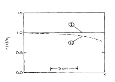
Figure 1: Measured ion number density profile in the target chamber for the experiment done by Chang et.al Chang . Continuous line denotes the profile if the perturbing structure is absent and the broken line denotes if it is present at the right edge. Reproduced with permission from Phys.Fluids 29,294(1986).Copyright 1986 American Physical Society.

From the steady state condition of ion continuity equation we get

$$\frac{\partial}{\partial\eta}[\tilde{n_{0}}\tilde{u_{0}}]=0,$$ (4)

where $\tilde{u_{0}}$ is the equilibrium ion velocity. Hence after integration $\tilde{u_{0}}$ can be determined as

$$\tilde{u_{0}}=\frac{c_{1}}{\tilde{n_{0}}}=c_{1}[1-\delta f_{0}],$$ (5)

where $c_{1}$ is an integration constant and higher order terms are neglected due to smallness.

Now from the steady state condition of the x component of momentum equation we get

$$\frac{\partial}{\partial\eta}[\tilde{u_{0}}^{2}+\tilde{\phi_{0}}]=0,$$ (6)

where $\tilde{\phi_{0}}$ is the equilibrium potential. After integration $\tilde{\phi_{0}}$ can be determined as

$$\tilde{\phi_{0}}=C_{2}-{\tilde{u_{0}}}^{2},$$ (7)

where $C_{2}$ is another integration constant. Choosing $C_{2}=c_{1}^{2}$, we get

$$\tilde{\phi_{0}}=2c_{1}^{2}\delta f_{0}(\eta),$$ (8)

where also higher order terms are neglected due to smallness. Choosing this, we can also see that the steady state condition of Poisson’s equation is also satisfied for these functions of $\tilde{\phi_{0}},\tilde{n_{0}}$ if the higher order terms are neglected due to smallness.

These equilibrium quantities are obtained self consistently from the fluid equations (1). To create equilibrium in a real experimental situation, external electric fields are imposed by using appropriate biasing arrangements inside the plasma. Details of the setup are found in JohnSaxena ; Dahiya2 . This also gives rise to steady drift that is space dependent in presence of density gradients.

The equilibrium electron number density is also inhomogeneous. The inhomogeneity of the equilibrium electron density can be expressed clearly from equation (1), from where we get

$$\tilde{n_{e0}}=e^{\tilde{\phi_{0}}(\eta)},$$ (9)

hence it is also inhomogeneous.

A reductive perturbation method is carried out with $\epsilon$ as the expansion parameter to obtain the two dimensional nonlinear evolution equation with weak transverse propagation. $\delta$ is a small parameter which is controlled externally to form the equilibrium density profile. For the sake of this work we take here $\delta$ to be $\approx\epsilon$.

All the variables are expanded as

$$n=1+\epsilon f_{0}(\eta)+\epsilon n_{1}(\xi,\eta,\lambda)+\epsilon^{2}n_{2}(\xi,\eta,\lambda)+...$$ (10)

$$\phi=2c_{1}^{2}\epsilon f_{0}(\eta)+\epsilon\phi_{1}(\xi,\eta,\lambda)+\epsilon^{2}\phi_{2}(\xi,\eta,\lambda)+...$$ (11)

$$u_{x}=c_{1}[1-\epsilon f_{0}(\eta)]+\epsilon u_{1}(\xi,\eta,\lambda)+\epsilon^{2}u_{2}(\xi,\eta,\lambda)+...$$ (12)

$$u_{y}=\epsilon^{\frac{3}{2}}v_{1}(\xi,\eta,\lambda)+\epsilon^{\frac{5}{2}}v_{2}(\xi,\eta,\lambda)+...$$ (13)

The set of stretched quantities and the expansion of the physical quantities given by (3)and (10)-(13) are used in the fluid equations (1) and the coefficients of different powers of $\epsilon$ are collected and set to zero.

At the lowest order $\bf{\epsilon}$, we get

$$\phi_{1}+2c_{1}^{2}f_{0}=n_{1}+f_{0}$$ (14)

At $\bf{\epsilon^{\frac{3}{2}}}$ we get,

$$(M-c_{1})\frac{\partial n_{1}}{\partial\xi}=\frac{\partial u_{1}}{\partial\xi},\ \ \frac{\partial\phi_{1}}{\partial\xi}=(M-c_{1})\frac{\partial u_{1}}{\partial\xi},$$ (15)

from where we obtain $(M-c_{1})n_{1}=u_{1}$ and $(M-c_{1})u_{1}=\phi_{1}$, where it is assumed that as $\xi\rightarrow\pm\infty$, $n_{1},u_{1}\rightarrow 0$. Using (14) and (15) we get $(M-c_{1})^{2}=1$ and $2c_{1}^{2}=1$ which gives $c_{1}=\frac{1}{\sqrt{2}}$ and $\phi_{1}=n_{1}=u_{1}$.

Because of the presence of drift, the equilibrium dispersion relation in the normalized variable $M$ is given by $M=1+\frac{1}{\sqrt{2}}$.

At $\bf{\epsilon^{2};}$ we obtain,

$$\frac{\partial v_{1}}{\partial\xi}=\frac{\partial\phi_{1}}{\partial\lambda},\ \ \frac{\partial^{2}\phi_{1}}{\partial\xi^{2}}+n_{2}=\phi_{2}+\frac{1}{2}(f_{0}+\phi_{1})^{2}$$ (16)

Finally at $\bf{\epsilon^{\frac{5}{2}}}$ order we get

$$-\frac{\partial n_{2}}{\partial\xi}+\frac{\partial}{\partial\xi}(-c_{1}f_{0}n_{1}+u_{1}n_{0})+\frac{\partial u_{2}}{\partial\xi}+\frac{\partial}{\partial\xi}(u_{1}n_{1})-c_{1}\frac{\partial f_{0}}{\partial\eta}+\frac{\partial u_{1}}{\partial\eta}+\frac{\partial v_{1}}{\partial\lambda}+c_{1}\frac{\partial f_{0}}{\partial\eta}+c_{1}\frac{\partial n_{1}}{\partial\eta}=0,$$ (17)

$$-\frac{\partial u_{2}}{\partial\xi}+\frac{\partial}{\partial\xi}(-c_{1}f_{0}n_{1})+\frac{\partial\phi_{2}}{\partial\xi}+n_{1}\frac{\partial}{\partial\xi}(n_{1})-c_{1}\frac{\partial f_{0}}{\partial\eta}+c_{1}\frac{\partial u_{1}}{\partial\eta}+2c_{1}^{2}\frac{\partial f_{0}}{\partial\eta}+\frac{\partial n_{1}}{\partial\eta}=0,$$ (18)

combination of which using (16), we get the final evolution equation

$$\frac{\partial}{\partial\xi}[(2+2c_{1})\frac{\partial n_{1}}{\partial\eta}+2n_{1}\frac{\partial n_{1}}{\partial\xi}+\frac{\partial^{3}n_{1}}{\partial\xi^{3}}]+\frac{\partial^{2}}{\partial\lambda^{2}}(n_{1})-2c_{1}f_{0}\frac{\partial^{2}n_{1}}{\partial\xi^{2}}=0,\ \$$ (19)

with $c_{1}=\frac{1}{\sqrt{2}}$, which is nothing but Kadomtsev-Petviashvili (KP) equation with an extra term appearing due to inhomogeneity . Here we have considered the simplest configuration of unmagnetized plasma with cold ions and isothermal electrons, but the similar equation with different coefficients can be derived for more complexities like ion temperature, presence of magnetic field etc for the chosen equilibrium ion number density profile. Note that, in KP2 the modified KP equation was derived, considering the fact that the scale length of the plasma inhomogeneity is much larger than the width of the soliton, and solitary wave solution is given for constant density gradient. Here, the equation (19) is the evolution equation for the nonlinear ion acoustic wave in two dimension where the unperturbed ion number density profile is taken to be slowly varying and weak.

Moving into the new frame

$$X=\xi+a(\eta),\ \ Y=\lambda,\ \ T=\eta,$$ (20)

with

$$a(\eta)=(\frac{c_{1}}{1+c_{1}})\int f_{0}(\eta)d\eta,$$ (21)

with $c_{1}=\frac{1}{\sqrt{2}}$. Equation (19) can be transformed to the standard constant coefficient KP equation

$$\frac{\partial}{\partial X}[\frac{\partial U}{\partial\tau}+6U\frac{\partial U}{\partial X}+\frac{\partial^{3}U}{\partial X^{3}}]+\frac{\partial^{2}U}{\partial Y^{2}}=0,\ \$$ (22)

where $U=\frac{n_{1}}{3}$ and $\tau=T/(2+2c_{1})$. This is a standard completely integrable KP equation which can be solved exactly giving soliton solutions. But due to the presence of the term $a(\eta)$ which is related to $f_{0}(\eta)$ via (21), in the new co-ordinate $X$, bending of solitons in the two dimensional plane occurs which will be shown in the next section.

III Bending of solitons

One soliton solution of KP equation (22) is similar as that of the soliton solutions of KdV equation Rec1 ; Rec2 with an extra transverse direction given by solitonkp1 ; solitonkp2 ,

$$U=\frac{k_{1}^{2}}{2}Sech^{2}[\frac{1}{2}(k_{1}X+m_{1}Y-\frac{k_{1}^{4}+m_{1}^{2}}{k_{1}}\tau)].$$ (23)

Expressing the solution in old variables we get,

$$n_{1}=(\frac{3k_{1}^{2}}{2})Sech^{2}[\frac{1}{2}\{k_{1}\xi+k_{1}a(\eta)+m_{1}\lambda-\frac{k_{1}^{4}+m_{1}^{2}}{2k_{1}(1+c_{1})}\eta\}],$$ (24)

with $c_{1}=\frac{1}{\sqrt{2}},$where $a(\eta)$ is given by (21) and $k_{1},m_{1}$ are arbitrary constants.

Due to the presence of the quantity $a(\eta)$ , related to the inhomogeneous ion number density , bending of soliton occurs.

Here the plasma is inhomogeneous due to the presence of the function $f_{0}(\eta)$. For different choices of $f_{0}$, the inhomogeneities are different. For the choice of $f_{0}=0$ the plasma becomes homogeneous which have the usual line solitons which is represented in FIG 2. Thus this trivial choice of $f_{0}$ in the equilibrium ion number density profile reproduces homogeneous plasma from the chosen inhomogeneity profile.

For different functional forms of $f_{0}$ dependent on the slowly varying co-ordinate $\eta$, different types of bending occurs, which are shown in FIG. 3.

For the sake of this problem, we have chosen $\delta=\epsilon$, which is the small perturbation parameter of our calculation. The solitary wave solution is independent of $\epsilon$, which is here taken to be $\delta$. The solution depends on the function $a(\eta)$ which is related to the function $f_{0}(\eta)$ through equation (21), causing the soliton to bend in the two dimensional plane. But the amplitude of the solitary wave solution remains constant.

Similarly, the two soliton solution is given by solitonkp1 ; solitonkp2 ,

$$n_{1}=6\frac{\partial^{2}}{\partial\xi^{2}}(\ln F_{2}),$$ (25)

with,

$$F_{2}=1+e^{\eta_{1}}+e^{\eta_{2}}+A_{12}e^{\eta_{1}+\eta_{2}},\ \ A_{12}=\frac{(K_{1}-K_{2})^{2}-(M_{1}-M_{2})^{2}}{(K_{1}+K_{2})^{2}-(M_{1}-M_{2})^{2}},$$

$$\eta_{1}=K_{1}[\xi+a(\eta)+\sqrt{3}M_{1}\lambda-\frac{(K_{1}^{2}+3M_{1}^{2})}{(2+2c_{1})}\eta],\ \ \eta_{2}=K_{2}[\xi+a(\eta)+\sqrt{3}M_{2}\lambda-\frac{(K_{2}^{2}+3M_{2}^{2})}{(2+2c_{1})}\eta],c_{1}=\frac{1}{\sqrt{2}}$$

where $K_{1},K_{2},M_{1},M_{2}$ are arbitrary constants. Bending of two soliton solution for different functional forms of $f_{0}(\eta)$ are also shown in FIG. 3. Since $f_{0}$ should reach zero value at $\eta=0$ following FIG.1, it has been chosen accordingly.

Now it is required to determine how much bending is taking place by varying $f_{0}$ i.e, what the condition is for larger bending.

Let us start from the one soliton solution (24). The amplitude of the ’Sech’ function is maximum when its argument goes to zero. For static case ($\xi$ = 0), the locus of the highest amplitude of the solution is of the form

$$\frac{1}{2}\{k_{1}a(\eta)+m_{1}\lambda-\frac{k_{1}^{4}+m_{1}^{2}}{2k_{1}(1+c_{1})}\eta\}=0,$$ (26)

where $c_{1}=\frac{1}{\sqrt{2}}$ .

Note that, for homogeneous plasma $f_{0}$ is zero making $a(\eta)$ to be also zero determined from equation (21). Hence the locus is straight line giving line solitons for homogeneous plasma.

Now taking derivative w.r.to $\eta$ twice in the above equation (26) we get

$$\frac{ds}{d\eta}=-\frac{k_{1}c_{1}}{m_{1}(1+c_{1})}\frac{df_{0}}{d\eta}$$ (27)

where $s=\frac{d\lambda}{\partial\eta}$ is the slope of the locus of the maximum amplitude. We choose $k_{1},m_{1}$ such that

$$\frac{ds}{d\eta}=\frac{df_{0}}{d\eta}$$ (28)

We see from the above equation that for higher value of RHS, rate of variation of slope will also be higher. Hence the slope of the maximum amplitude curve will vary large for traversing unit distance in $\eta$. Larger rate of variation of slope describes larger bending.

Hence for large bending of solitons to take place, the first derivative of $f_{0}$ w.r.to $\eta$ must also be high. This is incorporated in FIG 3 where bending of solitons occur for different choices of $f_{0}$.

For FIG 3(a)(i), if we increase the amplitude of $f_{0}$ then the parabola will steepen causing larger bending. Similar thing can be observed for FIG 3(b)(i) where the sine function becomes more rapid . Now if we increase the wave vector of $f_{0}$ in 3(b) then also the bending will become larger. Increase/decrease of both amplitude as well as wave vector of $f_{0}$ will increase/decrease the first derivative of $f_{0}$ causing more/less bending. The same analysis can be extended to the other figures 3(c), 3(d) too.

(a) One soliton                 (b) Two soliton

FIG.2: Static piture of one and two soliton solutions given by (24) and (25) of the two dimensional ion acoustic wave at $\xi=0$ for $k_{1}=1,m_{1}=1,K_{1}=K_{2}=\frac{1}{2},P_{1}=-P_{2}=\frac{2}{3}$ and $f_{0}=0$. Clearly, $f_{0}=0$ represents homogeneous plasma which is reproduced here from the chosen inhomogeneous ion number density profile. Line solitons which are found in the homogeneous plasma are also reproduced here for this trivial choice of $f_{0}$.

(a)(i) One soliton for $f_{0}=-\eta/3$         (a)(ii)Two soliton for $f_{0}=-\eta/3$

(b)(i) One soliton for $f_{0}=-4Sin(2\eta)$      (b)(ii)Two soliton for $f_{0}=-4Sin(2\eta)$

(c)(i) One soliton for $f_{0}=-(1+\sqrt{2})tanh(\eta)$      (c)(ii)Two soliton for $f_{0}=-(1+\sqrt{2})tanh(\eta)$

(d)(i) One soliton                     (d)(ii)Two soliton

for $f_{0}=-5(\sqrt{2}+1)(Sech(5(\eta-10)))^{2}$)           for $f_{0}=--5(\sqrt{2}+1)(Sech(5(\eta-10)))^{2}$)

FIG.3: Static piture of one and two soliton solutions given by (24) and (25) of the two dimensional ion acoustic wave at $\xi=0$ for $k_{1}=1,m_{1}=1,K_{1}=K_{2}=\frac{1}{2},P_{1}=-P_{2}=\frac{2}{3}$ and for the specified functions of $f_{0}$ which is related to unperturbed ion number density. The different functional forms of $f_{0}$ causes the phase of the solitary wave to change which causes bending in the two dimensional plane, whereas the amplitude remains constant.

Frycz and Infeld obtained the bending of soliton Bending1 by studying numerically the nonlinear stability analysis of KP equation. The characteristics of KP equation state that the initial condition must fulfill an infinite set of constraints if the solution is to remain localized. Just adding a perturbation to one soliton solution would violate this constraint. Thus bending is a natural perturbation which is a choice for initial condition of this numerical simulation. But in our work, the bending of solitons were obtained analytically showing dependence on $f_{0}$ which is related to inhomogeneous ion number density. We have exactly solved the KP equation (19) obtained for the two dimensional propagation of ion acoustic wave for weak and slowly varying inhomogeneity, related to the arbitrary function $f_{0}(\eta)$. Since we have transformed the evolution equation into a standard constant coefficient KP equation, its each and every solution faces the same phase modification controlled by $f_{0}$, causing the shape of the solution to change in the two dimensional plane. The amplitude of the soliton solutions is found to remain constant. This is in view of the weak and slowly varying inhomogeneous ion number density, so that all variations appear only in the phase of the soliton.

We see that the weak and slowly varying equilibrium potential, which exists in the plasma, is a function of $f_{0}$, varying along the x axis (i.e, $\eta$ axis). Hence due to this time independent potential an electric field develops which exerts force on the ions, constituting the soliton. But due to the inhomogeneity of the equilibrium potential function, different ions situated at different positions are attracted (or repelled) differently. Again an equilibrium ion drift velocity also exists, which is also directed in the x axis and inhomogeneous. Due to the superposed effects of the inhomogeneous equilibrium and also the time dependent quantities, the ions change their positions. This causes the ion acoustic soliton to bend in the two dimensional plane. Since the potential drop is weak as well as slow, the number of ions forming soliton do not change drastically. Hence the amplitude of the soliton remains constant causing its phase to vary with $f_{0}(\eta)$.

We see that, the one soliton solution of our evolution equation (19) contains the inhomogeneous function $a(\eta)$ in the phase. We see from the solution that the function reaches its maximum value when the phase factor turns to be zero. Hence as the soliton propagates in the two dimensional plane, $\eta$ changes causing $a(\eta)$ to change nonlinearly depending on $f_{0}(\eta)$. Now if we fix the time variable $\xi$, then the transverse variable $\lambda$ has to adjust itself in order to make the phase factor of the ”Sech“ function zero causing soliton bending.

These bending features of the solitons is very relevant and important in the context of inhomogeneous plasmas along with the other features like reflection, transmission etc. But such a feature has not been explored till now. We see in this work that if the equilibrium density variation is slow and weak, which is very close to the homogeneous value then these bending features can be seen. Hence a more accurate experiment could reveal such finer effects.

IV Conclusive remarks

In this work, we have obtained the bending of ion acoustic solitary wave in the two dimensional plane for the propagation in unmagnetized plasma with cold ions and isothermal electrons with weak and slowly varying density inhomogeneity. We have obtained a modified KP equation with an extra term arising due to inhomogeneous equilibrium ion density . We have exactly solved the KP equation giving a solitary wave solution in which the phase of the soliton gets modified by a function $f_{0}$, which is related to unperturbed ion density, causing soliton bending, where as the amplitude remains constant. The bending features of the solitons is very relevant and important in inhomogeneous plasma along with the other features like reflection, transmission etc. More accurate and precession experiment could reveal such finer and interesting features.

References

- (1) H. Washimi and T. Taniuti, Phys. Rev. Lett 17, 19 (1966).
- (2) F.F Chen Introduction to Plasma physics and controlled fusion , (Plenum Press, New York and London, 1984).
- (3) F. Aziz Thesis: Ion-acoustic solitons: Analytical, experimental and numerical studies, (2011) and references therein
- (4) N. Nishikawa and and P. K.Kaw Phys. Lett A 50, 455 (1975).
- (5) Y. Gell and L. Gomberoff, Phys. Lett. A 60, 125 (1977).
- (6) P.I John and Y.C Saxena Phys. Lett. A 56, 385 (1976).
- (7) N. N Rao and R. K Verma, .Phys. Lett. A 70, 9 (1979).
- (8) H.H Kuehl and K Imen, Phys. Fluids. 28, 2375 (1985).
- (9) H.Y Chang, S. Raychaudhuri, J.Hill, E.K Tsikis and K.E Lonngren, Phys. Fluids. 29, 294 (1986).
- (10) R. P Dahiya, P.I John and Y. C Saxena, Phys. Lett. A 65, 323 (1978).
- (11) G. Popa and M.Oertl, Phys. Lett. A 98, 110 (1983).
- (12) Y. Nishida, Phys. Fluids 27, 2176 (1984).
- (13) K.Imen and H.H Kuehl, Phys. Fluids 30, 73 (1987).
- (14) T. Nagasawa and Y. Nishida, Phys. Rev. Lett 56, 2688 (1986).
- (15) S. Yi, J.L Cooney, H.Kim, A. Amin, Y. El-Zein and K.E Lonngren, Phys. Plasmas 3, 529 (1996).
- (16) J.L Cooney, M.T Gavin, J.E Williams, D. W Aossey and K.E Lonngren, Phys. Fluids B 3, 3277 (1991).
- (17) H.H Kuehl Phys. Fluids 26, 1577 (1983).
- (18) K.Ko and H.H Kuehl, Phys. Rev. Lett 40, 233 (1978).
- (19) K. Ko and H.H Kuehl, Phys. Pluids 23, 834 (1980).
- (20) S.Singh and R.P Dahiya, Phys. Fluids B 3, 255 (1991).
- (21) S.Singh and R.P Dahiya, J.Plasma Phys 41, 185 (1989).
- (22) H.K Malik and R.P Dahiya, Phys.Plasma 1, 2872(1994)
- (23) D.K Singh and H.K Malik , Phys.Plasma 13, 082104(2006).
- (24) S.S Chauhan,H.K. Malik and R.P. Dahiya, Phys. Plasma 3, 3932 (1996).
- (25) D.K Singh and H.K Malik, Phys. Plasma 14, 062113 (2007).
- (26) D.Xiao, J.X Ma, Y.Li, Y.Xia and M.Y Yu, Phys. plasma 13,052308 (2006)
- (27) R.Kumar, H.K Malik, and S.Kawata, Physica. D 240,310 (2011)
- (28) H.K Malik , Phys. Lett. A 365, 224 (2007).
- (29) Q.Haque and S.Mahmood, Phys. Plasmas 15,034501 (2008)
- (30) H.K Malik, Phys. plasma 15,072105 (2008)
- (31) Jyoti and H.K Malik Phys. Plasmas 18, 102116 (2011).
- (32) H.K Malik, Jyoti and R.Kumar, J.Theor. Appl Phys 8, 123 (2014).
- (33) K.Singh, V.Kumar and H.K Malik Phys. Plasmas 12, 072302 (2005).
- (34) W.Duan and J.Zhao Phys. Plasmas 6, 3484 (1999).
- (35) I. Ibrahim and H.H Kuehl, Phys.Fluids 27,962 (1984)
- (36) W.F El-Taibany,M.M Selim, N.A El-Bedwehy and O.M Al-Abbasy, Phys. Plasmas 21, 073710 (2014).
- (37) A.P Misra and A.R Chowdhury Phys. Plasmas 13, 062307 (2006).
- (38) W.Masood Phys. Plasmas 17, 052312 (2010).
- (39) W.F.El-Taibany, M.Wadati and R. Sabry , Phys. Plasmas 14, 032304 (2007).
- (40) B.B Kadomtsev and V.I Petviashvili, Sov. Phys.Dokl.15, 539 (1970).
- (41) H.K Malik, S.Singh and R.P dahiya, Phys. Lett.A 195, 369 (1994).
- (42) W. Masood, Phys. Lett.A 373, 1455 (2009).
- (43) J.R Yang, X.Y Tang, X.N Gao, X.P Cheng and S.Y. Lou EPL 12, 45001 (2011).
- (44) L.P. Zhang and J.K. Xue Commun Nonlinear Sci Numer Simulat 15, 3379 (2010).
- (45) P. Frycz and E.Infeld , Phys. Rev. A 41,3375 (1990).
- (46) A.M Wazwaz Appl.Math.Comput, 190, 633 (2007).
- (47) M.J Ablowitz and D.E Baldwin, Phys.Rev.E 86, 036305 (2012).
- (48) H.Saleem, S.Ali and Q.Haque , Phys. Plasmas 22, 084509 (2015).
- (49) R.Jahangir, W.Masood, M.Siddiq, N.Batool and K.Saleem , Phys. Plasmas 22, 092312 (2015).