Model independent constraints on dark energy evolution from low-redshift observations
Abstract
Knowing the late time evolution of the Universe and finding out the causes for this evolution are the important challenges of modern cosmology. In this work, we adopt a model-independent cosmographic approach and approximate the Hubble parameter considering the Pade approximation which works better than the standard Taylor series approximation for . With this, we constrain the late time evolution of the Universe considering low-redshift observations coming from SNIa, BAO, , , strong-lensing time-delay as well as the Megamaser observations for angular diameter distances. We confirm the tensions with CDM model for low-redshifts observations. The present value of the equation of state for the dark energy has to be phantom-like and for other redshifts, it has to be either phantom or should have a phantom crossing. For lower values of , multiple phantom crossings are expected. This poses serious challenges for single, non-interacting scalar field models for dark energy. We derive constraints on the statefinders and these constraints show that a single dark energy model cannot fit data for the whole redshift range : in other words, we need multiple dark energy behaviors for different redshift ranges. Moreover, the constraint on sound speed for the total fluid of the Universe, and for the dark energy fluid (assuming them being barotropic), rules out the possibility of a barotropic fluid model for unified dark sector and barotropic fluid model for dark energy, as fluctuations in these fluids are unstable as due to constraints from low-redshift observations.
today
1 Introduction
The observed late time acceleration of the Universe is one of the most important milestones for research in cosmology as well as gravitational physics. It behoves us to go beyond the standard attractive nature of gravity and compels us to think out of the box to explain the repulsive nature of gravity that is at work on large cosmological scales. Whether the reason for this repulsive gravity is due to the presence of non-standard component with negative pressure in the Universe ( called dark energy) (Padmanabhan, 2003; Peebles Ratra, 2003; Sahni, 2002, 2005; Sahni et al., 2000) or due to large scale (infrared) modification of Einstein’s General Theory of Gravity (GR) (Barreiro et al., 2004; Burrage et al., 2011; Capozziello et al., 2005, 2011; Dvali et al., 2000; Freese et al., 2002; Nicolis et al., 2009; Nojiri et al., 2011, 2017), is not settled yet. Still, recent results by Planck-2015 (Ade et al., 2016a, b) for Cosmic Microwave Background Radiation (CMB), equally complimented by observations from Baryon-Acoustic-Oscillations (BAO) (Beutler et al., 2011, 2012; Blake et al., 2012; Lauren et al., 2013, 2014), Supernova-Type-Ia (SNIa) (Betoule et al., 2014; Perlmutter et al., 1997; Riess et al., 1998), Large Scale Galaxy Surveys (LSS) (Parkinson et al., 2012), Weak-Lensing (WL) (Heymans et al., 2013) etc, have put very accurate bound on the late time evolution of the Universe. It tells that the concordance CDM Universe is by far the best candidate to explain the present acceleration of the present Universe. But the theoretical puzzle continues to exists as we still do not know any physical process to generate a small cosmological constant, which is consistent with observations but is far too small (of the order of ) compared to what one expects from standard theory of symmetry breaking. Problem like cosmic coincidence also remains.
Interestingly, few recent observational results have indicated inconsistencies in the cosmological credibility of the CDM model. The model independent measurement of by Riess et al. (R16) (Riess et al., 2016) and its recent update (Riess et al., 2018), have shown a tension of more than with the measurement by Planck-2015 for CDM Universe (see also (Benetti et al., 2017)). Similarly, mild inconsistency in for CDM model is also observed by Strong Lensing experiments like H0LiCow using time delay (Bonvin et al., 2017). Subsequently (Valentino et al., 2018) have shown that such an inconsistency in CDM model can be sorted out if one goes beyond cosmological constant and assumes dark energy evolution with time. In recent past, Sahni et al.(Sahni et al., 2014) have also confirmed this dark energy evolution in model independent way using the BAO measurement. More recently, using a combination of cosmological observations from CMB, BAO, SNIa, LSS and WL, Zhao et al. (Zhao et al., 2017) have shown (in a model independent way) that dark energy is not only evolving with time but it has also gone through multiple phantom crossings during its evolution. Such a result, if confirmed by other studies, is extremely interesting as it demands the model building scenario to go beyond single scalar field models which, by construction, do not allow phantom crossing. It was first shown by Vikman (Vikman, 2005) and later by other authors in different contexts (Babichev et al., 2008; Hu, 2005; Sen, 2006). For a discussion on this topic in modified gravity, see (Bamba et al., 2009).
Although the majority of the studies to constrain the late time acceleration of the Universe assumes a specific model (either for dark energy or for modification of gravity), there have been attempts to study such issues in a model independent way. But in most of these model independent studies, the goal is to reconstruct the dark energy equation of state (Capozziello, 2006). There are two major issues for such studies. Reconstructing the dark energy equation of states needs a very precise knowledge about the matter energy density in the Universe. A small departure from that precise value can result completely wrong result for dark energy equation of state(Sahni et al., 2008). To avoid such issues, a number of diagnostics have been proposed that can independently probe dark energy dynamics without any prior knowledge about matter density or related parameters. Statefinders (Sahni et al., 2003; Alam et al., 2003) and Om Diagnostic(Sahni et al., 2008) are some of the most interesting diagnostics. Moreover, in a recent study, the limitation of using the equation of state to parametrize dark energy has been discussed(Scherrer et al., 2018). It is shown that the energy density of dark energy or equivalently the Hubble parameter are reliable observational quantities to distinguish different dark energy models.
In the literature, there are different approaches for model independent study for late time acceleration in the Universe. Some of the most studied approaches are Principal Component Analysis (PCA) (Huterer Starkman, 2003), Generic Algorithm (GA) (Bogdanos Nesseris, 2009; Nesseris Shafieloo, 2010), Gaussian Processes (GP)(Seikel et al., 2012; Shafieloo et al., 2012) etc. See (Vitenti & Penn-Lima, 2015) for a nice review on different approaches for reconstruction. Cosmographic approach to constrain the background evolution of the Universe is a simple and yet useful approach(Visser et al., 2004). Once the assumption of cosmological principle is made, it gives model independent limit for the background evolution of the Universe around present time. Given that the dark energy only dominates close to present time (except for early dark energy models), this approach is a powerful one to constrain the late time background evolution. The usual cosmographic approach involves Taylor expansion of cosmological quantities like scale factor and to define its various derivatives like Hubble Parameter (), deceleration parameter (), jerk (), snap () and so on and subsequently constrain these parameters (at present time) using different cosmological observations. This, in turn, can result constraints on the background evolution. This is completely model independent as no assumption of underlying dark energy model is needed. The major problem for this approach is that the Taylor expansion does not converge for higher redshifts and hence one cannot truncate the series at any order. To overcome this divergence problem for redshifts , the formalism of Pade Approximation (PA) for Cosmographic analysis was first proposed by Gruber and Luongo (Gruber Luongo, 2014) and later by Wei et al. (Wei et al., 2014). It was shown that the PA method is a better alternative than Taylor Series expansion, as the convergence radius of PA is larger than Taylor Series expansion. Hence, to constrain late time universe using Cosmography, PA is a reliable choice to extent the analysis to higher redshifts.
In most of the analysis, PA is applied to write down the dark energy equation of state(Gruber Luongo, 2014; Wei et al., 2014; Rezaei et al., 2017). Although this is a reasonable approach to constrain the late time evolution of the Universe, using dark energy equation of state has its own problems as discussed in earlier paragraphs. PA has been also used to approximate the energy density for the dark energy (Mehrabi Basilakos, 2018). Recently, PA is used to approximate the luminosity distance which is a direct observable related to SNIa observations (Aviles et al., 2014; Capozziello et al., 2018) . This gives a very clean constraints on late time Universe from SNIa observations as no further information is needed. But if one wants to use other observations related to background evolution, one first needs to calculate the Hubble parameter from and then use this to construct other observables.
Given the fact that all the low redshift observables are constructed solely from , it is natural to use PA to approximate the itself. Moreover, using PA for directly, one can allow both dark energy and modified gravity to model the background expansion.
In this work, we take into account this approach. We use (Pade Approximation of order (2,2)) for the Hubble parameter . Subsequently we use latest observational results from SNIa, BAO, Strong Lensing, H(z) measurements, measurements by HST as well as the angular diameter distance measurements by Megamaser Cosmology Project to constrain the late time evolution of the Universe. We first derive the observational constraints on various cosmographic parameters and later use those constraints to reconstruct the evolution of various equation of state, statefinder diagnostics and sound speed.
In Sec. 2, we describe the cosmography and the Pade Approximation; Sec. 3A is devoted to the description of different observational data used in the present study; in Secs. 3B-3E, we describe various results that we obtain in our study and finally in Sec. 4, we give a summary and outline perspectives of the method.
2 Cosmography and Pade Approximation
In Cosmographic terminology, the first five derivatives of scale factor are defined as the Hubble parameter (), the deceleration parameter (), the jerk parameter (), the snap () and the lerk ():
| (1) |
| (2) |
| (3) |
The Taylor Series expansion of the Hubble parameter around present time () is:
| (4) |
where . Here the derivatives of Hubble parameter can be expressed as
| (5) |
The series (4) does not converge for redshift 1. So, to increase the radius of convergence, we use Pade Approach (PA). The PA is developed using the standard Taylor Series definition but it allows better convergence at higher redshifts.We define the (N,M) order PA as the ratio:
| (6) |
has total number of independent coefficients. One can Taylor Expand and equate the coefficients to that for a generic function expanded as power series to get
| (7) |
| (8) |
Hence one can always write any function expanded in Taylor Series in terms of PA as:
| (9) |
In this work, we use to approximate the Hubble parameter . As mentioned in the Introduction, all the observables related to low-redshift observations are directly related to or they directly measure . So it is more reasonable that we use PA for itself. So we assume:
| (10) |
Remember that the “normalised Hubble Parameter ” is present in different expressions for observables like luminosity distance , angular diameter distance etc. Hence we apply PA to . While choosing Pade orders, we keep in mind that
-
•
The Pade function[NM] should smoothly evolve in all redshift ranges used for cosmographic analysis.
-
•
All Pade Approximations used, should give Hubble parameter positive.
-
•
The degree of polynomials for numerator and denominator should be close to each other.
-
•
While using a combination of datasets, the cosmographic priors should be chosen so that it does not provide divergences.
One can always redefine the parameters in (10) and set so that . Furthermore the parameters and are not physically relevant parameters. One can always relate them to physically relevant kinematic quantities like which represent cosmographic quantities for the cosmological expansion. For this, one needs to take different derivatives for given in (10) at and relate them to and solve and in terms of . Subsequently one gets:
| (11) |
where and are related to cosmographic pramaters () in equation (5).
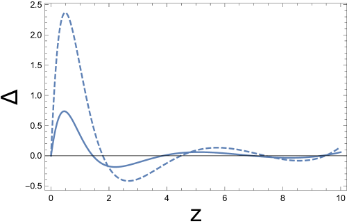
Before studying the observational constraints, we compare (10) with a fourth order Taylor Series expansion for which also contains four arbitrary parameters. We fit both to a CDM model given by . In Figure 1, we show which one fits the actual model better by plotting the difference between the fit and the actual model. One can clearly see, that in the redshift range , where the effects of repulsive gravity (and hence the late time acceleration) is dominant, the PA gives much better fit to the actual model than the Taylor series expansion and for PA, the deviation from actual model is always less than a percent. One should note that most of the low-redshift observational data are in this redshift range.
Furthermore, as one can see from Figure 1, the deviation from the actual model (in this case, from CDM) is maximum around , and this is true for Taylor series expansion as well as Pade. Given the fact that a large number of observational data are present around this redshift, it raises the obvious question that whether Pade is a good parametrisation to represent actual model around this redshift. But as one can see, the maximum deviation from the actual model, in case of Pade, is always less than although it is around for Taylor series expansion. As the accuracy of present observational data related to background universe, is still greater than , we should not worry about this peak in deviation around . We show in subsequent sections that Pade can indeed put sufficiently strong constrains on parameters related to background expansion around , which is enough to rule out a large class of standard dark energy behaviours.
3 Observational Constraints
3.1 Observational Data
To obtain observational constraints for six arbitrary parameters (four parameters in the expression for together with present day Hubble parameter and the sound horizon at drag epoch related to BAO measurements ) we use the following low-redshifts datasets involving background cosmology:
-
•
The isotropic BAO measurements from 6dF survey, SDSS data release for main galaxy sample (MGS) and eBoss quasar clustering as well as from Lyman- forest samples. For all these measurements and the corresponding covariance matrix, we refer readers to the recent work by Evslin et al. (Evslin et al., 2018) and references therein.
- •
-
•
Strong lensing time-delay measurements by H0LiCOW experiment (TDSL) (Bonvin et al., 2017).
-
•
The OHD data for Hubble parameter as a function of redshift as compiled in Pinho et al (Pinho et al., 2018).
-
•
The latest measurement of by Riess et al (R16) (Riess et al., 2016).
- •
3.2 Results
To carry out the detail statistical analysis to find the constraints on the cosmological expansion, we can proceed in two ways. We can directly use equation (10) with and find constraints on , or we can use the relations between and as given in (11) and use as parameters in our model. We study both the cases and find constraints on . The reconstructed in these two cases is shown in Figure 2. As one can see, both approaches have similar results for redshifts . But for higher redshifts (in particular for and above), there are disjoint regions between two cases beyond confidence interval, showing some amount of disagreement between the two approaches.
In our following calculations, we adopt the second approach where we use the parameters for our study as these are directly related to the cosmological expansion. As an example, assuming at all redshifts, directly implies the CDM behaviour. Similarly the sign change of parameter defines the deceleration-to-acceleration transition. There is no direct physical interpretation for the set of parameters .
The best fit and bounds on the parameters and for combination of all the datasets are and respectively showing that we do not have strong constraints for these two parameters from the current datasets.
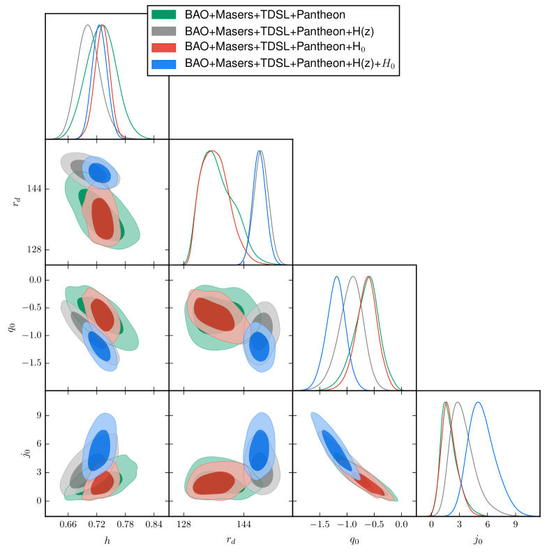
In Figure 3, we show the likelihoods and confidence contours for the rest of the cosmographic parameters, e.g., and the sound horizon at drag epoch that appears in the BAO measurements. Please note that in our calculations, we assume Km/s/Mpc. The best fit values along with bounds for these parameters are summarised in Table I. As one can see, although we can not put strong bounds on parameters and ( which are related to fourth and fifth order derivative of the scale factor), but the constraints on , and are pretty tight. In other words, the Pade can tightly constrain upto third derivative of the scale factor. This, in turn, can give very strong constraints on other derived parameters like , as well as different statefinder parameters, as shown in subsequent sections.
Following are the main results from Table I and Figure 3:
-
•
The low redshift measurements from BAO, Strong lensing, SNIa and angular diameter distance measurement by megamaser project, give constraint on which is fully consistent with R16 constraint on . Hence, in a model independent way, using low redshift observations, we confirm the consistency with measurement by R16 (Riess et al., 2016). If one adds measurement by R16 to this combination, the best fit value for shifts to the higher side resulting tensions with Planck-2015 measurements (Ade et al., 2016a) for CDM at ; in contrast, adding measurements to this combination, the best fit value for shifts to lower side and tension with Planck-2015 measurement reduces to less than . With combinations of all the data, the tension in with Planck-2015 result for CDM is . This result is completely model independent.
-
•
Without data, the allowed value for sound horizon at drag epoch as constrained by low-redshift data, is substantially smaller than from Planck-2015 for CDM model (Ade et al., 2016a). This is consistent with the recent result obtained by Evslin et al.(Evslin et al., 2018) using different dark energy models. Here we obtain the same result in a model independent way. But adding data shifts the constraint on on higher values making it consistent with the Planck-2015 measurement for CDM. With combination of all the datasets, the measured value of is fully consistent with Planck-2015 results for CDM. Consistency with Planck-2015 result for crucially depends on inclusion of measurements. Without , there is nearly inconsistency ( to be precise) with our model independent measurement for and that by Planck-2015.
-
•
With only low redshift measurements (BAO+SNIa+TDSL+Masers++), in a model independent way, we put strong constraint on deceleration parameter and it unambiguously confirms the late time acceleration.
-
•
One interesting result is for the jerk parameter . For CDM, always. Our result shows that is ruled out at confidence limit. There is a similar tension between measurement by R16 and Planck-2015 constraint on for CDM (Riess et al., 2016, 2018). Our study confirms similar tension with low redshifts measurements in a model independent way in terms of the jerk parameter .
-
•
From the likelihood plots and confidence contours in Figure 3, it is interesting to see that data pulls the results away from what one gets with rest of the datasets. This is true for all the parameters. The result for combination of all datasets strongly depends on data. We stress that this result is independent of any underlying dark energy or modified gravity models.
3.3 The role of the Equations of State
In the absence of spatial curvature, total energy density and the total pressure () of the background Universe can be expressed as:
| (12) |
where is the deceleration parameter of the Universe at any redshift. Using these, the effective equation of state of the background Universe is given by
| (13) |
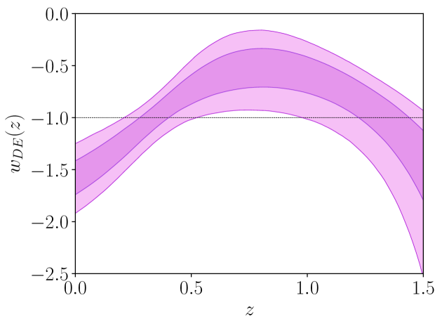
Using the constraints on the cosmographic parameters, we reconstruct the behaviour and its and allowed behaviors are shown in Figure 4. To compare with the Planck-2015 results for CDM(Ade et al., 2016a), we also show the reconstructed for CDM model using the constraints from Planck-2015. The figure shows the clear tension between the model independent behavior as constrained by low redshift data and the for CDM model as constrained by Planck-2015.
Note that, for an accelerating Universe, we should have . One can see in Figure 4, as one goes to past, the universe exits the accelerating regime and enters the decelerated period at around . But it also allows another accelerating period at high redshifts ( and higher) although decelerated universe is always allowed for . Adding data from high redshifts observations like CMB may change this behavior at high redshifts.

Although using (10), we constrain the overall background evolution of the Universe and it does not depend on any particular dark energy or modified gravity model, one can use the constraint on to reconstruct the dark energy equation of state . Assuming that the late time Universe contains the non-relativistic matter and dark energy, the dark energy equation of state can be written as:
| (14) |
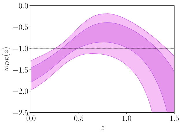

Here is the present day energy density parameter associated with the non-relativistic matter. As evident from this equation, one needs the information about to reconstruct . In our model independent approach using PA for , is not a parameter that we fit with observational data. So in order to reconstruct using (14), we assume three values for , e.g (). The model independent reconstructed is shown in Figure 5. One can observe following results from these plots:
-
•
For all three values of , cosmological constant ) is in more than tension with the reconstructed around present day.
-
•
For , this tension is also present for redshift range .
-
•
For and , around , there is also inconsistency with .
-
•
Irrespective of the value for , at low redshifts, the data allow only phantom behaviour () for .
-
•
For , a pure phantom or pure non-phantom is not allowed at all redshifts. There should be phantom crossing ( probably more than one).
-
•
For higher values of , although pure phantom behaviour is allowed at all redshifts, pure non-phantom behaviour is still not allowed at all redshifts.
-
•
Keeping in mind that a single canonical and minimally coupled scalar field model only results non phantom dynamics, our results show that all such scalar field models are in tension with low redshift observations. And this result is independent of choice of any dark energy model.
-
•
The overall behaviour of reconstructed for any values of , shows that the data prefer phantom crossing at low redshifts. As we discuss in the Introduction, crossing phantom divide with a single fluid non-interacting scalar field is difficult to achieve (Vikman, 2005; Babichev et al., 2008; Hu, 2005; Sen, 2006) ; our results show that such models are in tension with low-redshift observations. However, in case of an imperfect non-canonical scalar field model, this problem may be avoided, as shown by (Deffayet et al., 2010).
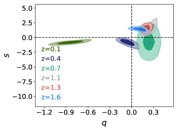
3.4 The Statefinder Diagnostics
Till now, we have constrained the cosmographic parameters from low-redshifts data in a model independent way. This, in turn, allows us to reconstruct the total equation of state of the Universe as well as the dark energy equation of state (assuming that late time acceleration is caused by dark energy) for specific choices of . But this does not allow us to pin point the actual dark energy model as there is a huge degeneracy between cosmographic parameters and different dark energy models. One needs some further model independent geometrical quantities that shed light on actual model dependence for dark energy. (Sahni et al., 2003) have introduced one such sensitive diagnostic pair , called “Statefinder Diagnostics” (Sahni et al., 2003; Alam et al., 2003). They are defined as:
| (15) |
| (16) |
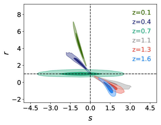
Here “prime” represents the derivative with respect to redshift. Remember the statefinder is same as the jerk parameter defined earlier. But we keep the original notation of statefinders as proposed by Sahni et al. (Sahni et al., 2003). One of the main goal of constructing any diagnostic is to distinguish any dark energy model from CDM and statefinders do exactly this as for CDM for all redshifts. Any deviation from this fix point in plane, signals departure from CDM behaviour. Moreover the different trajectories in plane indicate different dark energy models including scalar field models with different potentials, different parametrizations for dark energy equation of state and even brane-world models for dark energy ( we refer readers to Figure 1 and Figure 2 (Alam et al., 2003)).
We reconstruct the behaviours of and show different aspects of these reconstruction in Figure 6. Following are the results that one can infer from these plots:
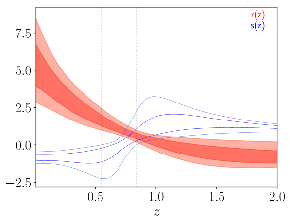

-
•
The first observation from Figure 6 is that there is no fixed point for all redshifts ruling out the CDM behaviour convincingly from low-redshift data. As one sees from the behaviour of as function of redshift ( Top, Left in Figure 6), there is a redshift range between where and are allowed simultaneously and in this redshift range CDM behaviour is possible. Outside this redshift range, CDM behaviour is ruled out.
-
•
The confidence contours in plane for different redshifts (Top, Right in Figure 6) give important clue about allowed dark energy models. If one compares this figure with Figure (1a).(Alam et al., 2003), one can easily conclude about possible dark energy behaviour allowed by the low-redshift data. It shows that in the past ( high redshifts), dark energy behaviours as given by different quintessence models ( including that with constant equation of state) are allowed, whereas around preset time ( low redshifts), models like Chaplygin Gas are suitable. In between, around , when we expect the transition from deceleration to acceleration has taken place, CDM is consistent with data.
The fact that no particular dark energy behaviour is consistent for the entire redshift range where low-redshift observations are present, is one of the most important results in this exercise and it poses serious challenge for dark energy model building that is consistent with low-redshift observations.
-
•
If one compares the contours in the plane (Bottom Right in Figure 6) with Figure 2 (Alam et al., 2003), one can see that at low redshifts, the “BRANE1” models ( as described (Alam et al., 2003)) are consistent which results phantom type equation of state. At higher redshifts and in the decelerated regime (), a class of brane-world models, called “disappearing dark energy” (refer to (Alam et al., 2003)) are possible that gives rise to transient acceleration. Hence, even if one models late time acceleration with various brane-world scenarios, it is not possible to fit the entire low-redshift range which we consider in our study, using a single brane-world description.
3.5 The Sound Speed
In literature, there has been number of studies assuming dark energy to be a barotropic fluid where pressure of the dark energy is an explicit function of its energy density:
| (17) |
Chaplygin and Generalized Chaplygin Gas, Van der Waals equation of state as well as dark energy with constant equation of state are few such examples which have been extensively studied in the literature. One interesting parameter associated with any barotropic fluid is its sound speed:
| (18) |
To ensure stability of the fluctuations in the fluid, we should have . Ensuring causality further demands (we refer readers to (Babichev et al., 2008) for situations where preserves causality). With a straightforward calculations, one can relate the statefinder with for barotropic fluid (Alam et al., 2003; Chiba Nakamura, 1998; Linder Scherrer, 2009):
| (19) |
The first equality of the above equation relates the statefinder to the sound speed of total fluid of the Universe, assuming that it is barotropic. This is relevant for unified models for Dark Sector where a single fluid describes both dark matter and dark energy (Bento et al., 2002; Billic et al., 2002; Davari et al., 2018; Mishra Sahni, 2018; Scherrer et al., 2004)(see also (Lim, 2010) for a UDM scenario with exactly). Here as defined in section 3C (we ignore the contribution from baryons which is negligible compared to dark matter and dark energy and has negligible contribution to background evolution).
The second equality relates statefinder to the sound speed of the dark energy , assuming that the dark energy is described by a barotropic fluid.
Let us first discuss the possibility of an unified fluid for the dark sector (Bento et al., 2002; Billic et al., 2002; Davari et al., 2018; Mishra Sahni, 2018; Scherrer et al., 2004). In Figure 6, we plot the redshift evolution of which shows that for , and for , . Moreover, the reconstructed as shown in Figure 4, shows that except around , where can be phantom (), always. Putting these results in the first equality in equation (19), shows that for redshifts , and one can not have stable fluctuations in the unified fluid. This is unphysical as such unified fluid can not form structures in our Universe. Hence our results with low-redshifts observations show that the unified model for dark sectors with stable density fluctuations, is not compatible with the low-redshift observations. Behaviour of for the total fluid is shown in Figure 7.
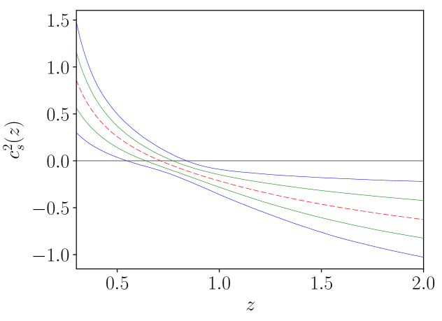
Next, we discuss the dark energy models as barotropic fluids and consider the second equality in equation (19). We already discuss the behaviour of for different redshifts in the previous paragraph. To reconstruct , we need to know the behaviour for . But without that also, one can get an estimate of the . For any physical dark energy model, always. Moreover, as shown in Figure 5 for the reconstructed for different , at low redshifts irrespective of the choice of . Hence at low redshifts for any dark energy barotropic fluid as constrained by low-redshift observations. We should stress that the dark energy dominates in the low-redshifts only and to have a consistent model for density perturbations in the Universe, we should take into account the perturbations in dark energy fluid even if it is negligible at some scales. But for barotropic dark energy fluid with , perturbation in dark energy sector is unphysical and we can not have a consistent model for density perturbation. Hence the barotropic fluid model for dark energy as constrained by low-redshift observations, is also not consistent with stable solutions for growth of fluctuations.
4 Conclusions
Let us summarize the main results, we obtained in this study:
-
•
We take a model independent cosmographic approach using order Pade Approximation for the normalized Hubble parameter as a function of redshift and subsequently constrain the background evolution of our Universe around present time using low-redshift cosmological observations. We stress that our approach is independent of any underlying dark energy or modified gravity model, hence independent of amount of matter content in the Universe.
-
•
The constraint on jerk parameter at present time , as well as the reconstructed statefinders , show that the CDM behaviour is inconsistent with low-redshift data.
-
•
Furthermore, the reconstructed total equation of state of the Universe as constrained by low-redshift data is shown to be inconsistent with the same as constrained by Planck-2015 data for CDM. This again confirms the apparent tension between low-redshift observations and the Planck-2015 results for CDM.
-
•
With the combination of SNIa+BAO+TDSL+Masers data, we obtain the model independent constraint on that is fully consistent with the measurement by R16.
-
•
For the full combination of dataset (SNIa+BAO+TDSL+Masers++), our model independent measurement for is Km/s/Mpc. This is in tension with Planck-2015 measurement for for CDM.
-
•
Assuming that the late time acceleration is due to the presence of dark energy, we also reconstruct the dark energy equation of state for three different choices of . This reconstruction also shows the inconsistency with cosmological constant irrespective of the value of .
-
•
The data allow only phantom model around present redshift. For , multiple phantom crossing is evident. For higher values of , pure phantom model is allowed although the overall shape of reconstructed confirms the existence of phantom crossing. This rules out single field minimally coupled canonical scalar field models for dark energy by low-redshift observations. This result is purely model independent.
-
•
Reconstruction of the statefinder diagnostics shows that one single model for dark energy (e.g. quintessence, chaplygin gas or brane-world scenarios) can not explain the behaviours for the entire redshift range where low-redshift data are available. For different redshift ranges, different dark energy behaviours are allowed. This poses serious challenge to dark energy model building.
-
•
Finally using the constraints on the statefinder , and , one can get useful constraint on sound speed for the total fluid in the Universe as well as for the dark energy fluid assuming that they are barotropic. For both the cases, for certain redshift ranges. This gives rise to unstable perturbations in these fluids which is unphysical. So one can conclude that low-redshift data is not consistent with barotropic models for unified dark sectors as well as with barotropic dark energy models.
To conclude, our model independent analysis with low-redshift data gives interesting insights for late time acceleration and, in particular, for the underlying dark energy behavior. In particular, the available dark energy models may not be suitable to explain the low-redshift data and we may need more complex models to explain the current set of data. In other words, the approach seems promising because, being model independent, could really discriminate among the various proposals in order to remove the degeneration of CDM where all models converge at late epochs. Finally the indication that a single fluid model, generally used to account for the whole dynamics, seems not sufficient: it could simply mean that coarse-grained models are not realistic in view to achieve a comprehensive description of the Universe history.
Finally, in our study, we used the set of parameters (which are directly related to cosmography) instead of the actual parameters of the Pade approximation in Eq.(10). The results involving these two sets of parameters do not fully agree for redshifts as shown in Figure 2. So the results and tensions for higher redshifts, ( and above) quoted in our study, may change if one uses the set of parameters. But as shown in all the reconstructed plots for different cosmological quantities, the uncertainty in these quantities are already quite large for redshift and above. In conclusion, one needs to be very careful about these facts while considering results in the redshift range and above.
5 Acknowledgement
SC acknowledges COST action CA15117 (CANTATA), supported by COST (European Cooperation in Science and Technology). SC is also partially supported by the INFN sezione di Napoli (QGSKY). Ruchika is funded by the Council of Scientific and Industrial Research (CSIR), Govt. of India through Junior Research Fellowship. AAS acknowledges the financial support from CERN, Geneva, Switzerland where part of the work has been done. The authors thank Anto I. Lonappan for computational help. We acknowledge the use of publicly available MCMC code “emcee” (Foreman-Mackey et al., 2013).
References
- Ade et al. (2016a) Ade P. A. R. et al., 2016a, Astron. Astrophys., 594, A13
- Ade et al. (2016b) Ade P. A. R. et al., 2016b, Astron. Astrophys., 594, A14
- Alam et al. (2003) Alam U., Sahni V., Saini T. D. and Starobinsky A. A., 2003, MNRAS, 344, 1057
- Aviles et al. (2014) Aviles A., Bravetti A., Capozziello S., Luongo O., 2014, Phys. Rev. D, 90, 043531
- Babichev et al. (2008) Babichev E., Mukhanov V. and Vikman A., 2008, JHEP, 0802, 101
- Babichev et al. (2008) Babichev E., Mukhanov V. and Vikman A., 2008, JHEP, 02, 101
- Bamba et al. (2009) Bamba K., Geng Chao-Qiang, Nojiri S., and Odintsov S. D., 2009, Phys. Rev. D 79, 083014
- Barreiro et al. (2004) Barreiro T. and Sen A. A., 2004, Phys. Rev. D, 70, 124013
- Benetti et al. (2017) Benetti M.,Graef L. L., Alcaniz J. S. ,2017, JCAP 1704, 003
- Bento et al. (2002) Bento M. C., Bertolami O. and Sen A. A., 2002, Phys. Rev. D, 66, 043507
- Betoule et al. (2014) Betoule M. et al., 2014, [SDSS Collaboration],Astron. Astrophys. 568, A22
- Beutler et al. (2011) Beutler F. et al., 2011, Mon.Not.Roy.Astron.Soc., 416, 3017
- Beutler et al. (2012) Beutler F. et al., 2012, Mon.Not.Roy.Astron.Soc., 423, 3430
- Billic et al. (2002) Billic N., Tupper G. B., Viollier R. D., 2002, Phys. Lett. B, 535, 17
- Blake et al. (2012) Blake C. et al., 2012, Mon.Not.Roy.Astron.Soc., 425, 405
- Bogdanos Nesseris (2009) Bogdanos C. and Nesseris S., 2009, JCAP, 0905, 006
- Bonvin et al. (2017) Bonvin V. et al., 2017, Mon.Not.Roy.Astron.Soc., 465, 4914
- Burrage et al. (2011) Burrage C., De Rham C., Heisenberg L., 2011, JCAP, 1105, 025
- Davari et al. (2018) Davari Z. and Malekjani M. ,Artymowski M., 2018, arXiv:1805.11033 [gr-qc]
- Capozziello (2006) Capozziello S., Cardone V. F. , Elizalde E., Nojiri S. and Odintsov S. D., 2006, Phys. Rev. D 73, 043512
- Capozziello et al. (2005) Capozziello S., Cardone V. F. and Troisi A., 2005, Phys. Rev. D, 71, 043503
- Capozziello et al. (2018) Capozziello S., D’Agostino R., Luongo O., 2018, JCAP, 1805, 008
- Capozziello et al. (2011) Capozziello S., De Laurentis M., 2011, Phys. Rept. 509, 167
- Chiba Nakamura (1998) Chiba T. and Nakamura T.,1998, Prog. Theor. Phys., 100, 1077
- Deffayet et al. (2010) Deffayet C. , Pujolas O. , Sawicki I. and Vikman A., 2010, JCAP, 1010, 026
- Dvali et al. (2000) Dvali G. R., Gabadadze G. and Porrati M., 2000, Phys. Lett., B 485, 208
- Evslin et al. (2018) Evslin J. ,Sen A. A, Ruchika, 2018, Phys. Rev. D, 97, 103511
- Foreman-Mackey et al. (2013) Foreman-Mackey D., Hogg D. W. , Lang D. and Goodman J. , 2013, “Emcee: The MCMC Hammer”, Publ. Astron. Soc. Pac., 125, 306
- Freese et al. (2002) Freese K.and Lewis M., 2002, Phys. Lett., B540, 1
- Gao et al. (2016) Gao F. et al., 2016, Astrophys. J., 817, 128
- Gomez-Valent Amendola (2018) Gomez-Valent A. and Amendola L., 2018, JCAP, 1804, 051
- Gruber Luongo (2014) Gruber C. and Luongo O., 2014, Phys. Rev. D., 89, 103506
- Heymans et al. (2013) Heymans C. et al., 2013, MNRAS, 432, 2433
- Hu (2005) Hu W., 2005, Phys. Rev. D, 71, 047301
- Huterer Starkman (2003) Huterer D. and Starkman G. , 2003, Phys. Rev. Lett., 90, 031301
- Kuo et al. (2013) Kuo C. et al., 2013, Astrophys. J., 767, 155
- Lauren et al. (2013) Lauren A. et al., 2013, Mon.Not.Roy.Astron.Soc., 427, 3435
- Lauren et al. (2014) Lauren A. et al., 2014, Mon.Not.Roy.Astron.Soc., 441, 24
- Lim (2010) Lim E. , Sawicki I. and Vikman A. , 2010, JCAP, 1005, 012
- Linder Scherrer (2009) Linder E. V. and Scherrer R. J. , 2009, Phys. Rev. D, 80, 023008
- Mehrabi Basilakos (2018) Mehrabi A. and Basilakos S., 2018, arXiv:1804.10794 [astro-ph.CO]
- Mishra Sahni (2018) Mishra S. S. and Sahni V., 2018, arXiv:1803.09767 [gr-qc]
- Nesseris Shafieloo (2010) Nesseris S. and Shafieloo A.,2010, MNRAS, 408, 1879
- Nicolis et al. (2009) Nicolis A., Rattazzi R.and Trincherini E.,2009, Phys. Rev. D, 79, 064036
- Nojiri et al. (2011) Nojiri S., Odintsov S. D.,2011, Phys. Rept. 505, 59
- Nojiri et al. (2017) Nojiri S., Odintsov S. D. and Oikonomou V. K., 2017, Phys. Rept. 6921
- Padmanabhan (2003) Padmanabhan T., 2003, Phys. Rep. 380 235
- Parkinson et al. (2012) Parkinson D. et al., 2012, Phys. Rev. D, 86, 103518
- Peebles Ratra (2003) Peebles P. J. E. and Ratra B., 2003, Rev. Mod. Phys. 75 559
- Perlmutter et al. (1997) Perlmutter S. et al., Astrophys. J., 483, 565 (1997);
- Pinho et al. (2018) Pinho A. M. , Casas S. and Amendola L., 2018, arXiv:1805.00027[astro-ph.CO]
- Reid et al. (2017) Reid M. J. et al.,2017, Astrphys. J., 767, 154
- Rezaei et al. (2017) Rezaei M., Malekjani M., Basilakos S., Mehrabi A. and Mota D. F., 2017, Astrophys. J., 843, 65
- Riess et al. (1998) Riess A. G. et al., 1998, Astron. J., 116, 1009
- Riess et al. (2016) Riess A. G. et al., 2016, Astrophys. J., 826, 56
- Riess et al. (2018) Riess A. G. et al., 2018, Astrophys. J., 853, 126
- Riess et al. (2018) Riess A. G. et al., 2018, arXiv:1804.10655 [astro-ph.CO]
- Sahni (2002) Sahni V., 2002 astro-ph/0202076
- Sahni (2005) Sahni V., 2005, astro-ph/0502032
- Sahni et al. (2003) Sahni V.,Saini T. D. ,Starobinsky A. A. and Alam U., 2003, JETP. Lett., 77, 201
- Sahni et al. (2008) Sahni V., Shafieloo A. and Starobinsky A. A., 2008, Phys. Rev. D, 78, 103502
- Sahni et al. (2014) Sahni V., Shafieloo A. and Starobinsky A. A., 2014, Astrophys. J., 793, L40
- Sahni et al. (2000) Sahni V. and Starobinsky A.A., 2000, Int. J. Mod. Phys. D9 373
- Scherrer et al. (2018) Scherrer R. J., 2018, arXiv:1804.09206 [astro-ph.CO]
- Scherrer et al. (2004) Scherrer R. J., 2004, Phys. Rev. Lett., 93, 011301
- Seikel et al. (2012) Seikel M. , Clarkson C. and Smith M., 2012, JCAP, 1206, 036
- Sen (2006) Sen A. A., 2006, JCAP, 0603, 010
- Shafieloo et al. (2012) Shafieloo A. , Kim A. G. , Linder E. V. , 2012,Phys. Rev. D, 85, 123530
- Valentino et al. (2018) Valentino E. , Linder E. and Melchiorri A. , 2018, Phys. Rev. D, 97, 043528
- Vikman (2005) Vikman A., 2005, Phys. Rev. D, 71, 023515
- Visser et al. (2004) Visser M., 2004, Class. Quant. Grav., 21, 2603
- Vitenti & Penn-Lima (2015) Vitenti S. D. P. and Penn-Lima M. ,2015, JCAP, 09, 045
- Wei et al. (2014) Wei H., Yan Xiao-Peng., Zhou Ya-Nan, 2014, JCAP, 1401, 045
- Zhao et al. (2017) Zhao Gong-bo et al., 2017, Nat.Astron., 1, 627