Charge conserving approximation for excitation properties of crystalline materials.
Abstract
A charge conserving approximation scheme determining the excitations of crystalline solids is proposed. Like other such approximations, it relies on “downfolding” of the original microscopic model to a simpler electronic model on the lattice with pairwise interactions. A systematic truncation of the set of Dyson - Schwinger equations for correlators of the low energy (downfolded) model of a material, supplemented by a “covariant” calculation of correlators lead to a converging series of approximates. The covariance preserves all the Ward identities among correlators describing various condensed matter probes. It is shown that the third order approximant of this kind beyond classical and gaussian (Hartree - Fock) is precise enough and due to several fortunate features the complexity of calculation is surprisingly low so that a realistic material computation is feasible. Focus here is on the electron field correlator describing the electron (hole) excitations measured in photoemission and other probes. The scheme is tested on several solvable benchmark models.
I Introduction
Calculation of the band structure and response functions of crystalline material with determined chemical composition is one of the most important theoretical problems in condensed matter physics. However computing the electronic excitations and spectra of a stoichiometric chemically well-defined compounds with significant correlations from first-principles continues to be a major challenge in computational material science. Historically the Kohn-Sham density functional methodKohn (DFT) opened the door to such calculations. The basic many-body Hamiltonian is that of the jellium model (neglecting the phonon degrees of freedom). The method approximates the many-body physics by a noninteracting electrons is periodic potential. It is successful to map out general features of the band structure of numerous crystalline solids.
However, DFT is not accurate enough in the most important (for condensed matter physics) range of energies near the Fermi level for which many-body effects are important. Kohn-Sham eigenvalues have been used to interpret the single particle excitation energies measured in direct and inverse photoemission experiments. Reasonable results were obtained in simple metals, however, when the excited state properties of semiconductors and insulators are concerned, ambiguities between different DFT approaches (for example the exchange correlation functional) and significant deviations from the measured characteristics appear. A well-known example is the systematic large (up to factor 2) underestimation of the fundamental band gaps of semiconductors in LDA.
Therefore to zoom in on this energy range relevant for description of the electromagnetic, thermal and other condensed matter properties that is dominated by the excitation effects, a two step strategy is employed. DFT is used as a first step to determine the “downfolded” modelCasula , or “effective low energy” electronic model containing most of the relevant information. The model is defined on the unit cell lattice with spectrum described by the two body electronic Greens function with relevant bands indexed by . The number of atomic orbitals (including spin) should not be not large with the long range interaction described economically by an “photon Greens function . The very high or low energy modes (tens of eV away from Fermi level) are thus “integrated out”. To be successful the downfolding typically utilizes the maximally localized DFT wavefunctionsVanderbilt . The downfolded model described in more detail below is dynamical and thus does not allow the description of the effective low energy system by a Hamiltonian, so the Matsubara action is employed.
The downfolded model is still very complicated and a number of numerical (like Monte Carlo (MC) supplemented by dynamical mean field, DMFKotliar ) and field theoretical methods like GWHedin and FLEXSavrasov18 were developed. The most popular analytic method to solve the downfolded (effective low energy) model sufficient for an accurate calculation of the condensed matter properties has been the use of the GWHedin . The GW method corrects the band gaps and other quasi-particle properties, such as lifetimes in a wide range of weakly correlated semiconductors and insulators. Hybertsen and LouieHedin showed that applying GW approximation as a first order perturbation to the Kohn-Sham quasiparticles of DFT (so called one shot or ) provides an accurate description of the photoemission spectra described by the electron Greens function. However the method has well-known limitations.
First the full nonlinear set of GW equations is notoriously costly to solve. It, in fact, has been carried out in full only for a limited number of models like the electron gasHolm and the results are not dramatically better and sometimes worse than those of various GW simplifications like the one shot . This is a set of nonlinear equations with generally a large number of solutions. Second, it appears that results are worse in moderately coupled materials and definitely inaccurate or even misleading in strongly coupled electronic systems. One therefore is required either to combine it with other methods (like Monte Carlo) or to go beyond the GW approximation.
It has been proven difficult to systematically improve the GW approximation by including higher-order Feynman diagrams, the so-called vertex corrections. While extensions of the GW approach have been developed for specific applications such as the cumulate expansion of the time dependent Green’s functions for the description of plasmon satellitesGunnarson , or the Bethe - Salpeter approach BS . Particularly troublesome problem for various extensions has been to conform to the most basic principles like charge conservationBaym . Many approaches violate the so-called Ward identities that are consequences of the symmetries of the system. As a result, there exists currently no universal, viable and applicable “beyond-GW” approachTakada .
A general method to preserve the Ward identities in an approximation scheme was developed long time agoKovner in the context of field theory as the covariant gaussian approximation (CGA) to solve an unrelated problem in quantum field theory and superfluidityKovner2 . A non-perturbative variational gaussian method originated in quantum mechanics of atoms and molecules in relativistic theories like the standard model of particle physics had several serious related problems. First, the wave function renormalization required a dynamical description. Second, the Green’s functions obtained using the naive gaussian approximation violated the charge conservation. In particular the most evident problem is that the Goldstone bosons resulted from spontaneous breaking of continuous symmetry are massive. The method is thus considered dubious and/or inconsistent. Both problems were solved by an observation that the solution of the minimization equations are not necessarily equivalent to the variational Green’s function. This constitutes the covariant gaussian approximation or CGAKovner .
The method was compared with available exact results for the S-matrix in the Gross-Neveu modelGN (a local four Fermion interactions in 1D Dirac excitations recently considered in condensed matter physics) and with Monte Carlo simulations in various scalar models, see ref.Wang17, for detailed description and application to thermal fluctuations in superconductors in the framework of the Ginzburg - Landau - Wilson order parameter approachRMP ). Applied to the electronic field correlator in electronic systems, CGA becomes roughly equivalent to Hartree - Fock approximation that is generally not precise enough. It’s covariance might improve the calculation of the four fermion correlators like the density- density, but to address quantitatively photoemission or other direct electron or hole excitation probes, a more precise method is needed.
The CGA approach is just the second in a sequence of approximations based on covariant truncations of the DS equations in which cumulant of third and higher order are discarded. One can continue to the next level by retaining the third cumulant (discarding the fourth) etc. We term this approximation covariant cubic approximation, CCA. The covariance still preserves all the Ward identities, so it is conserving according to definition of ref. Baym, . Up to now methodology of this kind has not been applied to more microscopic description of realistic condensed matter systems.
The subject of the present paper is to inquire whether is possible and computationally feasible. It is shown using several solvable benchmark models, that the third order approximation is precise enough. Its complexity when applied to a realistic material calculation is estimated. The focus is on the electron (hole) excitations correlator described by the electron field correlator that in turn can be compared to photoemission data and other probes, although higher correlators like the density - density (or conductivity) can be also considered as shown in refs. Kovner, ; Wang17, .
The paper is organized as follows. In section II the sequence of covariant approximations developed using the simplest possible case: the one dimensional integral. Next in section III the third approximation of these series, CCA is applied to a ( invariant) statistical Ginzburg - Landau - Wilson modelLubensky describing various statistical mechanical systems like the Ising chain in terms of low energy (effective) bosonic field theory. The results are compared with exact (at low dimension) and MC simulations (higher dimensionality). In section IV the general formalism for downfolded electronic system describing crystalline materials is presented and applied in Section V to some low dimensional benchmark systems like the single band Hubbard model. In Section VI contains an estimate of complexity of application of CCA to a realistic material and conclusions.
II Hierarchy of conserving truncations of DS equations
The main ideas behind the covariant approximants are presented in this section in the simplest possible setting. Later the third in a series of such approximant for a many - body system will be considered in some detail.
II.1 An exactly solvable “bosonic” model: one dimensional integral
To clearly present the general covariant approximation scheme, we will make use of the simplest nontrivial model: statistical physics of a one dimensional classical chain that is equivalent to the quantum mechanics of the anharmonic oscillator in the next section. Our starting point here will be the following “free energy” as a function of a single (real) variable
| (1) |
Here and represent spectrum and “couplings” respectively, while the“source” or “external field” will be used to calculate correlations. The exact partition function of just one “fluctuating” bosonic variable isfootnote1
| (2) |
Correlators (Greens function) are defined as
| (3) |
so that
| (4) | |||||
While the odd correlators in the symmetric case vanish, the exact one - body correlator is
| (5) |
where the partition function itself is
| (6) |
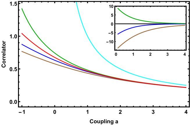
The dependence of the correlator on for , is given in Fig.1 as a red line.
Another important set of quantities include cumulantLubensky defined via the “effective action”, the Legendre transform, , . The (two particle irreducible) cumulants
| (7) |
The well known relations between the cumulants and correlators used below are given in Appendix A.
II.2 The set of the DS equations
The first in a series of the DS equations, the off shell “equation of state” (ES, the term “off shell” in this paper meaning that the quantity depends on the external source ) is
| (8) |
Using the connected correlatorsLubensky (marked by subscript ) and eventually cumulants, one obtains
| (9) |
Higher order DS equations in the cumulant form are obtained by differentiating the equation above. The second DS equation is,
while the next is more complicated,
| (11) |
Furthermore the fourth DS (disregarding odd condensates, as they will not be required for our purposes) has a form:
| (12) |
The infinite set of DS equations is not useful in practice unless a way to decouple higher order equations is proposed. For example, one can ignore all the and terms in Eq.(9) and Eq.(II.2) so that the remaining unknown variables can be solved by the two on - shell () “truncated” DS equations (or equivalently the minimization equations in gaussian variational method): the shift equation and gap equation. This simple truncation procedure called gaussian approximation, as stated before, is not symmetry - conserving. Fortunately a simple improvement based on gaussian approximation, the covariant gaussian approximationWang17 (CGA), includes “chain corrections” to the two - body cumulant by taking functional derivative of the off - shell (keep finite source ) shift equation with respect to . The chain correction is then explicitly calculated by taking derivative of the gap equation.
In the following several subsections, a hierarchy of approximations defined as truncations of the DS equations as well as their variational interpretations are introduced. The CGA scheme will immediately follow when one is familiar with the classical and gaussian approximations. Let’s start with the simplest truncation: classical approximation evaluation.
II.3 Classical approximation
The classical approximation consists of neglecting the two and higher body correlators in the equation of state, Eq.(9),
| (13) |
so that the second and higher equations are decoupled from the first. Then the “minimization equation”, that is just the on-shell () ES, is solved. For there are typically several solutions of this equation footnote1 . Here restricting discussion here to , and the solution has .
Note that despite the fact that the minimization principle involved only the one - body cumulant, , one can still calculate the higher cumulants within the classical approximation. These are given by derivatives of the source with respect to in truncated ES, Eq.(9),
| (14a) | |||
| The full correlator in momentum space is just . The independence on for , is given in Fig. 1 as the cyan line, compared to the exact correlator (red), emphasizes the fact that the classical approximation correlator ignores the quartic term and thus might be useful (as a starting point of the “loop expansion”, see Section IV) only at small . | |||
The classical minimization equation can be interpreted variationally as optimizing the free energy Eq.(1). One can do better. Why not optimize also the connected correlator in addition to the VEV of the field ? This is the gaussian approximation idea proposed early on in the context of quantum mechanics and develop in field theory in eighties of the last century, see ref.Stevenson, and references therein.
II.4 Covariant gaussian approximation
Now we drop in the first two DSE all the three field cumulants (equivalently connected correlators). This leaves us with the coupled equation for the two variational parameters
| (15) | |||||
The first equation is obviously obeyed for , while the second takes a form
| (16) |
Within the covariant approximation described in detail in ref.Wang17, , the connected correlator is equal to . The symmetric solution exists for any , however spurious first order transition to the “symmetry broken” solution occurs at .
The dependance of the correlator for on in the range is given in Fig. 1 as the brown line. It is significantly better than classical, yet underestimates the correlator up to 15%, see inset at . This value already approaches the spurious transition at . The approximation becomes better in the perturbative region at large , as will be discussed later.
II.5 The third order (cubic) approximation
Continuing the same idea the neglect of fourth and higher correlators. The ES of state is now exact,
| (17) |
while the next two are approximate (truncated),
| (18) | |||||
| (19) |
The first (taken on shell, ) equations are solved by . Then the gap equation coincides with the gaussian, Eq.(16), with the same solution Eq(15). However, according to the general covariant approach outlined in ref. Wang17, , the calculation of correlators starts with the off shell ES, as in original definition in the second line of Eq.(7).
For example correction to the inverse correlator is the first derivative of Eq.(17). After making the derivative
| (20) |
one substitutes the truncated quantities and their derivative on shell:
| (21) |
The first two terms, according to the gap equation, Eq.(18), are inverse of the truncated propagator , so that the cumulant can be conveniently written as
| (22) |
In the last term, so called “chain” correction,, is naturally obtained from the differentiation of the (off shell multiplied by ) truncated third minimization equation, Eq.(19):
| (23) |
Here the general relation between cumulant and connected functions, was used. Unlike the gap equation, this equation is linear, so that,
| (24) |
and finally
| (25) |
Now the spurious second order transition to a “symmetry broken” solution occurs at a lower negative value than the CGA one. This is a trend. Higher approximation symmetric phase solution works in the increasingly large portion of the parameter space. The dependance of the correlator for on in the range is given in Fig. 1 as the green line. CCA now overestimates the correlator up to 10% at , see inset.
II.6 The fourth order (quartic) approximation
The truncation is not needed now for the first two DSE, so that the ES stays as in Eq.(17) and the gap equation takes the full form
| (26) |
while the next two are approximate. The third will be required off shell,
| (27) |
The last term is needed only on - shell, thus all the odd correlators can be omitted:
| (28) |
The first and the third minimization equations are still trivially satisfied as long as odd correlators vanish. The second and the fourth equations on - shell for the two even connected correlators , take (upon multiplication by and respectively) the “Bethe - Salpeter” form
| (29) | |||||
| (30) |
The gap equations, solved for allows to obtain a cubic equation,
| (31) |
for .
The cumulant , given by the derivative of the ES in terms of the chain is the same as for the cubic approximation, Eq.(24). However the chain equation, although still linear,
| (32) |
now gives
| (33) |
The cumulant now takes a form
| (34) |
Its inverse for is given in Fig. 1 as the blue line over the range . It underestimates the exact results by just 5% at , as shown in the inset. The general trend is that the approximants oscillate converging the exact result. Let us now discuss the convergence of these approximations to the exact correlator, Eq.(5) and their asymptotic at weak and strong coupling.
III Testing the covariant approximations on statistical physics models
In this section the results of the covariant approximants outlined above are compared with exact values (or in more complicated cases numerical simulations that is known to be reliable) for the bosonic invariant Ginzburg - Landau -Wilson models. The formalism is generalized to the lattice model of arbitrary dimension . We start with .
III.1 Convergence of the first four approximants to the exact correlator of the bosonic toy model.
The “partition function” of the toy model, used in the previous section, Eq.(2), despite having two coefficients, and , has just one independent parameter: . Since and we first assume , only is considered in Fig.1. The figure indicates that the sequence of approximants converges quite fast. To make this more quantitative, let us first compare asymptotic.
| approximants | weak coupling expansion | strong coupling expansion | b=1 | b=4 | b=16 |
| exact | |||||
| classical (I) | 114 | 259 | 559 | ||
| cov. gauss (II) | -7.2 | -10.3 | -12.3 | ||
| cov. cubic (III) | 3.1 | 5.5 | 7.3 | ||
| cov. quartic (IV) | -2.0 | -3.7 | -4.9 |
At small coupling , the expansion up to are given in Table I. One observes that the expansion is exact to order , where is the order of the approximation. A more surprising result is that the leading incorrect term is within of the correct value. For example for the cubic approximation the coefficient is compared with exact , the quartic approximation the coefficient is compared with exact .
At strong coupling the situation is a bit different. At any order of the expansion parameter the coefficient converges to the exact at large . In between (see values and in Table I). The deviation from exact (given in %) does not exceed 13% for covariant gaussian (typical of course to numerous “mean field” approaches), 8% for covariant cubic and 5% for covariant quartic. Note that the deviations would increase dramatically if a noncovariant (naive or variational) version is usedWang17 .
To conclude, increasing the rank of the covariant truncation approach increases precision at a price of more complexity. Now we consider the same Ginzburg - Landau - Wilson (GLW) model in higher dimensions . Although an exact correlator is unknown, it can be calculated numerically with practically arbitrary precision as in ref. Wang17, and compared with classical CGA and CCA approximations.
III.2 Statistical mechanics of the D - dimensional model
The statistical physics in terms of the (real) order parameter of the Ising universality classLubensky ; Kleinert ; Rothe is defined by the statistical sum on a hypercube lattice :
| (35) |
The lattice laplacian in dimensions is
| (36) |
The hopping direction is denotedRothe ; Kleinert by . Periodicity of each direction is assumed, with “lattice spacing” setting the length scale .
The temperature will set the energy scale . This can be regarded as a lattice version of the Ginzburg - Landau - Wilson actionLubensky ; Kleinert and is a generalization of the toy model of the previous subsection, in that the position index appears. In fact we transform it to the momentum space
| (37) |
so that the
| (38) | |||||
where is the number of points of the lattice.
The off shell truncated DS equations now take a form:
| (39) | |||||
Here summations over should understood as an Einstein summation index are assumed. Minimization equations in the symmetry unbroken phase phase reduces to the gaussian one, solved in ref.Wang17, .
The symmetric solution of the minimization equations reduce, as in the toy model, to the solution of the gap equation, that due to translation invariance
| (40) |
is algebraic
| (41) |
There . Correction to correlator subsequently is
| (42) |
where the chain is defined as . The translation invariance of the chain, , allows to write the second equality.
Let us turn now to the chain equations, obtained, as in the toy model, from (functional) derivative of the third DSE, Eq.(39). It reads
| (43) |
One notices that, due to locality of the interaction, in addition to the fact that is a “spectator”, on the RHS of the equation only sum over the last momentum in appears. Since we need only summed in the correction to the inverse correlator, Eq.(42), we sum up the equation over the last index , . Using the fish integral , the chain equation finally takes a form:
| (44) |
This set of linear equations is solved numerically. Let us start with a simpler 1D case that allows an simpler solution (and can be interpreted as quantum mechanics of the anharmonic oscillator).
III.3 D=1 chain (or quantum mechanical anharmonic oscillator)
The case corresponds to the GLW type description of the Ising chain. It is equivalent to the quantum mechanics of the anharmonic oscillator for small limit, see Eq.(35). This case, although not solvable analytically, allows numerical solution with unlimited precision, and is compared with covariant gaussian and cubic approximations first. A more general case of arbitrary is compared with Monte Carlo simulations.
III.3.1 Low temperature compared with the quantum anharmonic oscillator
In 1D the temperature in statistical physics of classical chain can be reinterpreted as and the quantum anharmonic oscillator,
| (45) |
discretized partition function (at temperature . For very large the correlator approaches the correlation of for the ground state of the quantum anharmonic oscillatorKleinert . The thermal fluctuations in this interpretation are replaced by the quantum ones. Classical approximation and CGA for this model for the correlator and some composite correlators was worked out in ref. Wang17, .
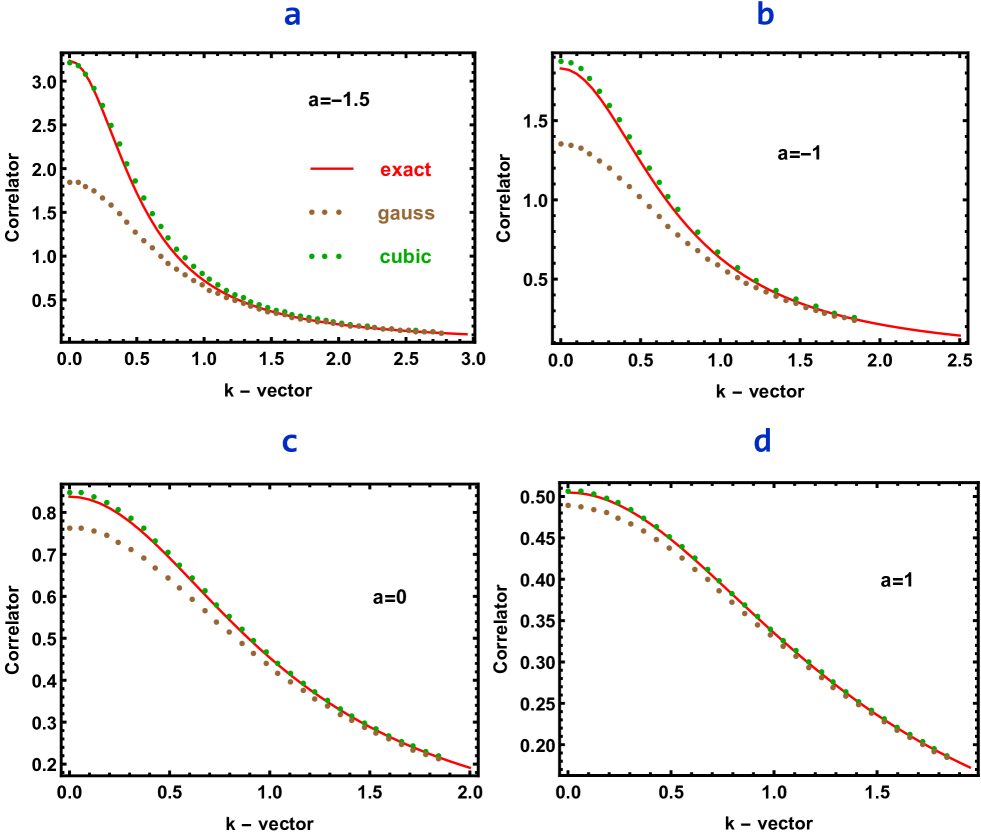
The distance between spatial points should be a small as possible, so we take . The coupling is fixed at (can be rescaled to this value), while . The “exact” correlator (the red line in Fig. 2) was calculated as
| (46) |
and are eigenvalues and eigenstates of Hamiltonian of Eq.(45). We used to ensure continuum limit. One observes that the convergence to exact value is generally faster than in , see Fig.1. Cubic overestimates much less than the gaussian underestimates the correlator for all k - vectors. For example the , Fig. 2d, CCA is within 1% for the whole range of k - vectors. Even for negative values of CCA is very precise away from the spurious phase transition of the gaussian approximation at . In was shown in ref. Wang17, that the instanton calculus is effective only for , so that the approximations work in the region where no other simple approximation scheme exists. For the value of that is not small, one cannot rely on continuum limit quantum mechanics, so the Monte Carlo approximate method is employed.

III.3.2 Monte Carlo simulation of the GLW action on finite chain
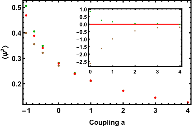
In Fig.3 the results of the MC calculation of the average correlator in space are shown for in the range to and . The sample size was with (with periodic boundary condition). The standard Metropolis algorithm is usually inefficient for because of the large autocorrelation of the samples. The autocorrelation however can be reduced to a large extent by combining the Metropolis algorithm with the cluster algorithm. This is done by using Wolff’s single-cluster flipping methodBrower . Each cycle of the Monte Carlo iteration contains a single cluster update of the embedded Ising variables, followed by a sweep of local updates of the original fields using Metropolis algorithm. The calculated integrated autocorrelation time was typically less then second in a usual desktop PC. With such reduced autocorrelation, the statistical error for a run containing several cycles after reaching equilibrium is already small enough.
The CCA was computed for the same sample size using Mathematica (green dots in Fig.3. The results are reminiscent of the quantum mechanical continuum limit with maximal deviations at of 6% for CGA (underestimate) reduced to 2% for CCA (overestimate). A naive expectation is that, when dimensionality is increased or interaction that becomes longer range, the mean field - like approximations of the type considered here, the range of applicability grows. Although in the present paper nonlocal interactions (most notably Coulomb interactions in insulators, semiconductors) is not considered here, the GLW model have been studied by MC in higher dimensions (D=2,3)Arnold and it will be compared with the CCA calculation below.
III.4 CCA for the D=2 GLW model compared to Monte Carlo simulation
Similar calculation has been performed in 2D for the sample size . Here in the same region of parameter space, , , the fluctuations influence is less pronounced, so the cluster method is not required in the case not being too near critical state. This is above the second order phase transition (lower critical dimensionality for the spontaneous symmetry breaking is ) at deduced from the correlator as function of distance between the two points. The correlator was averaged over 128 points . Results for are presented (as the red dots) in Fig. 4. The precision estimate for is 0.2%. Thermalization was achieved after MC steps and were used for measurement.
Gaussian approximation for was calculated on the same lattice, see brown dots in Fig. 4. As was noticed long agoStevenson , the transition at is a spurious weakly first order with finite excitation mass on the symmetric side (symmetric solution exists for any ). This fact was one of the problems of the approximation at the early stages of its development. The spurious first transition however is very close to the second order transition point found in MC. CGA underestimates the MC result by 2.5% at , see inset.
The CCA value for in the same range was computed for the same sample size using Mathematica (green dots in Fig. 4) using parallel computing. The results, green dots in Fig.4, overestimate the MC value by at . Of course in the perturbative region (large ), as before the gaussian approximation is one loop exact, while the cubic is two - loop exact. Generally 2D convergence is better than in 1D and is expected to further improve in 3D.
In the next section we formulate the CCA for a general fermionic model and apply it to develop a calculational scheme for a general computation of the electron Green function for an arbitrary crystalline material.
IV Covariant cubic approximation for the electrons in a crystalline solid
Covariant gaussian approximation for a fermionic system interacting via local four - Fermi term has been considered long time ago and compare wellGN with exact scattering matrix found by the factorization methodsZamolodchikov in some 1+1 dimensional relativistic models (the Gross - Neveu model, known in condensed matter physics as the Schrieffer-Su-Heeger model, was considered). Here we formulate the third order covariant approximation, CGA, that surprisingly turns out to be not much more complicated computationally. The additional effort is to solve large systems of linear equations.
IV.1 Cubic approximation in general four - fermion interaction model.
Let us start with a rather general case using abstract notations, to demonstrate the general structure of the method. All the characteristics of fermionic degrees of freedom (electrons) like location in space, time, charge, band index (including spin) etc described by (real) grassmanian numbers are lumped into one index . The four - Fermi interaction model (described in more detail for “downfolded” models electrons on lattice with effective interactions in the next subsection) is defined by the Nambu - Matsubara “action” and “statistical sum”:
| (47) | |||||
This formalism is slightly more general than the complex grassmanian numbers approachNO , in which a conjugate pair is describing annihilation or creation of a charged fermion. The Nambu approach is often used in description of superconducting state has an advantage of transparency due to explicit antisymmetry of all the grassmanians. In particular the “hopping amplitudes” and the interaction are totally antisymmetric in generalized indices.
Let us adjust the definitions of correlators to the fermionic case, paying attention to order of the grassmanian variables and their derivatives. Cumulants and connected correlators of fermions are defined as
| (48) | |||||
The description of CCA closely follows the steps described for bosons above. The first is “truncation” of the infinite set of Dyson-Schwinger equations.
IV.1.1 First three DS equations and their truncation
Differentiating the effective action (Legendre transform of ) off shell (namely in the presence of the fermionic source ), the equation of motion is
| (49) |
Note that the antisymmetry of the coefficients in the Nambu real grassmanian used here greatly simplifies the expressions compared to the complex grassmanian formalism. Similarly the second DS, using repeatedly the relation,, is
| (50) |
As in the bosonic CCA of the previous section, the fourth correlator term was dropped from the truncated equation (this is the meaning of ”). Similarly all the terms containing fourth and fifth cumulants will be dropped from the third DS equation:
| (51) |
These equations will be used twice. First the on - shell version, , the minimization equations are solved and then, the (CCA) correlator is computed from a derivative of the ES using via chain rule.
IV.1.2 Minimization equations: just the Hartree - Fock approximation
In fermionic systems one obviously does not have nonzero expectation values for (on - shell, ) odd cumulants, namely vanish on - shell. Unlike in the bosonic theories this does not hinge on the preservation of symmetries. As a consequence the first and the third minimization equations are trivially satisfied. The gap equation on shell is (we do not mark “tr” for the variational on-shell green function in this section for the simplicity of notation):
| (52) |
The first (matrix) equality has a sign opposite to that for bosons. The equation is just the Hartree - Fock (HF) self - consistency conditionNO . This means that the complexity of the only nonlinear operation within the CCA scheme for fermions coincides with the complexity of a presumably less precise CGA (equal for calculation of the one body correlator to the HF approximation). The additional complexity arises only to the fact that within CCA the connected correlation does not coincides with the truncated correlator, as we have seen in the previous section and will be assessed later.
Therefore we turn to the derivation of the correction formally similar to that in the bosonic model, Eq.(22).
IV.1.3 Correction to correlator
The CCA inverse correlator is derivative of the off - shell ES, Eq.(49):
The on - shell nonzero contributions to in the fermionic model are written via correction as:
| (54) |
The first term are just the truncated inverse correlator (or the covariant gaussian inverse correlation) in view of the gap equation, Eq.(52).The chain, a derivative of truncated three - point connected correlator will be denoted by
| (55) |
The “chain” is found from the derivative of the third DS equation, Eq.(51).
IV.1.4 The chain equation
Differentiating the “connected version” of the third truncated DS equation,
| (57) | |||||
one obtains on - shell:
One can prove that the chain is antisymmetric under only. For example . This is typical for “truncated” (non - covariant) quantities that was observed already in CGAGN ; Wang17 .
The first important observation is that the chain equation is linear, as in the bosonic case. An additional important observation is that the parameter is a “spectator”, so, since it is an external index in the correlator itself, Eq.(54), one do not have to run over all its values.
IV.1.5 Most economic linear combination of chains: V-chains
The chain equations although linear are very numerous. On the other hand, a glance at the expression for the correction to the inverse correlator, Eq.(54), shows that only linear combinations are required. A general question arises whether some linear combinations are “closed” on themselves. We have already noticed “spectators” in Eq.(IV.1.4).
After some “trial and error”, it turns out that the following combinations of the chains are more convenient. Defining the convenient chains combination as
| (59) |
the correction becomes a “trace”:
| (60) |
where is the summation index, and and indices are also summation indices in the equation below. The “V - chain” (antisymmetric in the second and third index) obeys the corresponding linear combination of the chain equations:
| (61) |
This allows to solve the set of linear equations less times and in addition to use the “reduce” routines.
Let us now apply the rather abstract formalism to a sufficiently general charge conserving electronic system.
IV.2 Charge conserving electron system with pairwise interaction
IV.2.1 Down folding of the microscopic Hamiltonian. Measurement of the electron correlator by photo - emission.
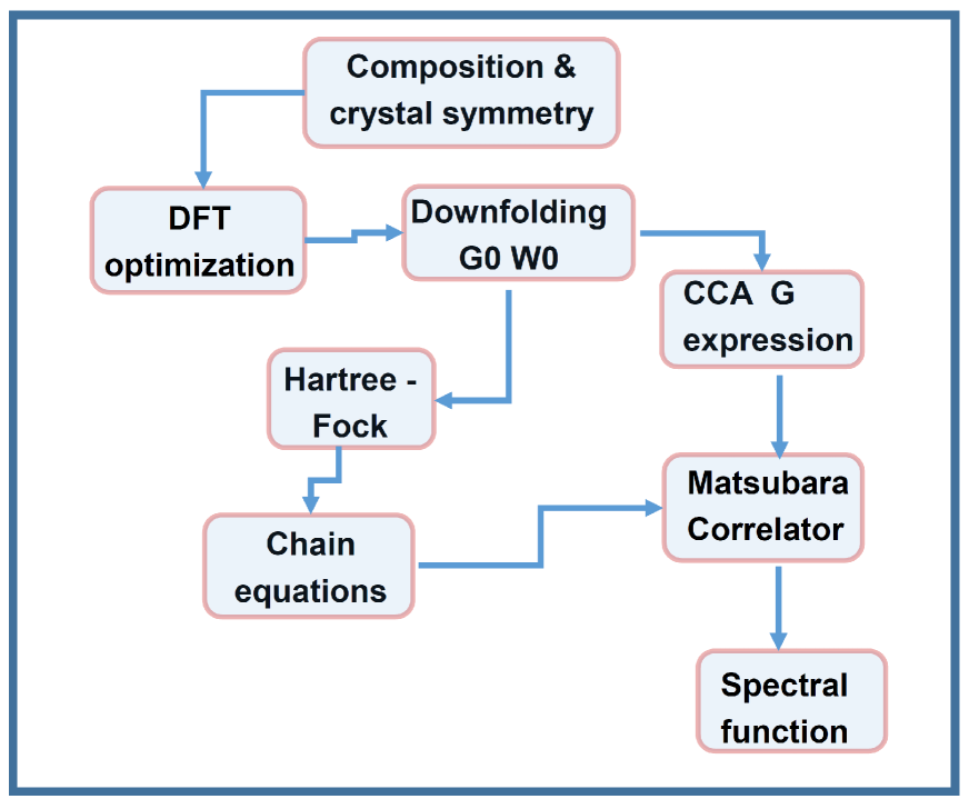
Electronic system in a crystal on the microscopic level is described by a many - body Hamiltonian with Coulomb interactions between electrons and very slowly moving nuclei (considered typically as an external potential). The problem of the determination of the electromagnetic, thermal and other condensed matter properties that incorporate the excitation effects, is divided into two steps, see Fig. 5. First DFT is used to calculate coefficients of the effective low energy (meaning close to the Fermi level within 1eV or so) “down - folded” modelCasula . The bands far from the Fermi level and irrelevant parts of the original Hilbert space are thus projected out.
Although there is a certain ambiguity what electronic model contains most of the relevant information, there exists a reasonable choice for insulators and semiconductors that still allows GW, DMFT, and as will be shown next, CCA. The crucial novel feature of the CCA is its manifest charge conservation (covariance).
The model is defined on a lattice with sufficiently large unit cell. The downfolded spectrum is given by the two body electronic Greens function with relevant bands indexed by . The number of retained atomic orbitals (including spin) should not be not be too large for CCA (see estimates in the discussion section). The typically rather long range unscreen Coulomb interactions are described economically by a “photon Greens function” . The restriction of the effective downfolded four fermion interaction to being pairwise of the density - density type is not obvious. CCA in general four - Fermi interaction is not feasible at presently available computational power. To be successful the downfolding generally utilizes the maximally localized DFT wavefunctionsVanderbilt .
Recently the electronic Greens function is being “measured” rather directly by various photo - emission probes like ARPES - angle resolved photo - emission spectroscopy. This is especially important for novel clean crystalline materials, many of them low dimensional semiconductors and so called Weyl semi - metals like , graphene etc. The Matsubara frequency correlator calculated within CCA should therefore be analytically continued to the spectral weight and density of states to be compared with experiments and other methods, see Fig. 5. With this in mind a sufficiently general modelNO ; Guiliani is defined formally next.
IV.2.2 Matsubara action for the general downfolded model.
The Matsubara action of the general pairwise interacting downfolded electron model has a formNO :
| (62) | |||||
Charge conservation is explicit here. This should be matched with fully symmetrized Grassmanian form, Eq.(47):
| (63) |
Here is the charge (Nambu) index that originate from the creation and annihilation operators in the many - body HamiltonianNO . The rest of the indices are contained in . The “band” index includes spin. The interaction is of the density - density form and thus . The result is:
| (64) | |||||
| (68) |
This model is now amenable to the CCA approximation scheme. In the present paper only the correlator (one body correlator or green function) is computed.
IV.2.3 CCA equations for the correlator
For charge unbroken case (no superconductivity) some simplifications occur. All the “charges” correlators like vanish on - shell. The only correlators remaining are , related by where is the summation index. General Nambu gap equation, Eq.(52) in an electric charge preserving system takes a form:
| (69) |
The chain correction to the inverse propagator, Eq.(22) in our case becomes,
| (70) |
Only two charge components of the chain appear here due to the antisymmetry of the chain. Let us denote them as diffuson and cooperon chains in analogy to similar expressions in diagrammatic many - body physicsAkkermans :
| (71) |
For these two quantities the general chain equation, Eq.(IV.1.4), closes:
Solution and application of these equations greatly simplifies when the translational symmetry is utilized.
IV.2.4 Translation invariance
In addition to charge conservation we assume the electronic system to be invariant under a crystalline translation symmetry and time translations. The model of relevant number of bands (including spin) constructed on the lattice with periodic boundary conditions in each direction, to keep notations as simple as possible, the square lattice is assumed with lattice spacing defining the unit of length . The points therefore are , (dimensionality). At temperature the Matsubara (Euclidean) time is also discretized in the range and is antiperiodicNO .
Therefore the electron field is carrying two types of indices , the band index will be consistently written as a superscript, while the space - time index will be eventually substituted by integer valued wave number and the Matsubara frequency , so that we map . Definitions of the discrete Fourier transform (FT) of the complex grassmanian field is
| (73) |
Now enumerates the space - time components of the energy-momentum basis. Translation invariance (energy and momentum conservation) leads to the following FT for the correlators:
| (74) |
where . For the inverse propagator it is convenient to define FT by
| (75) |
where is the Matsubara time step, so that . Consequently tunneling and interaction potentials FT are,
| (76) | |||||
where has bosonic Matsubara frequency.
Using these definitions the HF equation, Eq.(69), becomes:
| (77) |
The correction to the inverse propagator takes a form
| (78) |
where
| (79) | |||||
Finally the chain equation are (the spectator frequency-wave-vector indices are and )
with being the only summation index. To test the CCA in a fermionic model, one should apply the method to an exactly solvable one. Exact solution exists for sufficiently small in the case of local interaction - Hubbard model. We therefore apply CCA to the case of Hubbard model and compare it to the exact diagonalizationED (ED) in the case of (quantum dot) and 1D with small finite .
V Fermionic benchmarks: quantum dot and one dimensional Hubbard model.
V.1 The CCA approximation in D - dimensional one band Hubbard model.
V.1.1 The model, gap and chain equations.
The single band Hubbard model is defined on the dimensional hypercubic lattice. The tunneling amplitude to the neighbouring site in any direction is denoted in literature by . We chose it to be the unit of energy . Similarly the lattice spacing sets the unit of length and . The Hamiltonian is:
| (81) |
The chemical potential and the on - site repulsion energy are therefore given in units of the hopping energy The “band” index therefore takes two values . The hopping direction is denoted by as in statistical physics modelRothe ; Kleinert of Eq.(36). The density and its spin components are with . External magnetic field makes the electrons polarized. At half filling .
The discretized Matsubara action isNO ,
| (82) |
where and the “slice size” in anti - periodic Matsubara time is , where is temperature and is the number of points in the compact time axisNO . Therefore the hopping matrix in frequency-momentum space of the corresponding Matsubara action, Eq.(62) is
| (83) | |||||
while the interaction is just a constant:
| (84) |
The gap equation, Eq.(69), in this case takes a form:
| (85) | |||||
where the dimensional notations like will be used to simplify the expressions. In the range of parameters considered in the present paper the spin rotation symmetry along the z axis will be assumed unbroken (A larger symmetry appears at zero magnetic fieldKorepin , which is not discussed here since we focus initially on the “symmetry” unbroken phases). The most Ansatz is .
Therefore the only two nontrivial diagonal components (denoted by ) of the truncated inverse propagator are
| (86) |
where the bar over the spin index means that the spin was flipped. The couple of algebraic self consistent equations finally is:
| (87) |
and is easily solved numerically.
The set of chain equations greatly simplified exactly as in the bosonic model since the interaction is local. One requires only coincident coordinates for the cooperon and diffuson defined in Eq.(71). Moreover the remaining spin symmetry (spin along the z axis) limits the nonzero spin components. Generally Pauli symmetry demands that for cooperon with fixed spectator spin , the only nonzero choice is . For the symmetry leaves three choices , and . The resulting set of chain equations in Fourier space is:
| (88) | |||||
Here summation over bosonic () and fermionic () frequencies/momenta are assumed.
The CCA correlator, Eq.(78) in this case is:
| (89) |
It was calculated (using C++ program on parallel computer) for the cases of the toy model (quantum dot) and for sufficiently small so that exact diagonalization is possible.

V.2 Fermionic toy model: quantum dot
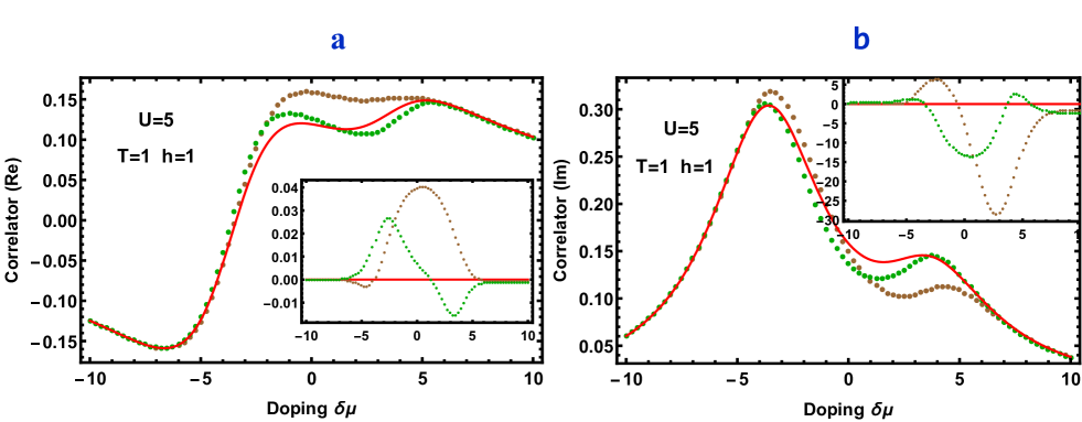
Let us first consider an exactly solvable model of just a single site (“quantum dot”). Recently artificial systems like that with several sited Hubbard model were manifacturedqdexp and the experimental results were compared with exact diagonalization (ED). The space indices are absent in the model, so that the space-time index stands for the frequency after Fourier transform. The model can be solved with the result for the correlator of the up spin being:
| (90) | |||||
This is presented as a red lines in Fig. 6. In Fig. 6a the real part of the Matsubara correlator in wide range of doping for is given, while Fig. 6b exhibits the imaginary part. Temperature and magnetic field were fixed at , . One observes a very good agreement not only in perturbative domains for large absolute value of (far away from half filling. The maximal deviations are , (real part) and , (imaginary part) for CGA and CCA respectively, see insets. In Fig. 7 the same is given for a strong coupling . The agreement is worse, by still have maximal deviations are , (real part) and , for CGA and CCA.

V.3 Comparison of results with exact diagonalization for one dimensional Hubbard model
The one dimensional case is considered for simplicity and availability of exact results utilizing the exact diagonalizationED for reasonably large values of . The largest lattice we have used to exactly calculate Green’s function was (so that the number of fermionic degrees of freedom is ) and avoided using the Lancos algorithms to diagonalize large matrices, since temperature range in units of the hopping parameter of the Hubbard model is considered. The relatively high temperature allows lower to obtain precision of for the CCA calculation using the “naive” discretization of Eq.(82). Larger lattices were treated by the exact diagonalization, however in these calculations typically only spectrum and expectation values were computed. To compare with CCA the Matsubara time correlators are required. These are more difficult to compute. The program was written in Mathematica.
The program for CCA was written in C++ and utilizes parallel computing on a node cluster and large memory of . The doping range was for the band with (in units of the hopping parameter). Temperature and magnetic field were fixed at , . The results for are presented in Fig. 8 and 9 for intermediate, and strong, , couplings respectively. As in Figs. 8,9 a show the real part of the Matsubara correlator, while b - the imaginary part. One observes a very good agreement not only in perturbative domains for large absolute value of (far away from half filling. The maximal deviations are , (real part) and , (imaginary part) for CGA and CCA respectively for , see insets In Fig. 8. In Fig. 9 the same is given for a strong coupling for . The agreement is worse, by still have maximal deviations are , (real part) and , for CGA and CCA. Generally results are similar to that in for the relatively low value of .
Till now the application of CCA to a number of solvable field theoretical models was considered to gauge its precision and complexity. It is not the purpose of the present paper to apply the method to a realistic material, however below we estimate the mathematical/computational complexity of such a calculation.
VI Discussion and conclusions
VI.1 Complexity of the CCA computation for a realistic material
Naive estimate of the computational complexity of covariant third order approximation is misleading due to the following three observations of the formalism presented in Section IV.
1. Since the odd order fermionic correlators vanish, the only variational parameter is still the truncated correlator, namely the most complicated third equation, Eq.(57), is trivially satisfied in the fermionic model (unlike in bosonic model in the symmetry broken phase that is indeed too complicated). Moreover the only on shell equation coincides with HF.
2. The chain equations, 79, are all linear. We do not have a proof, but it seems to be a common feature for both covariant gaussian and CCA.
3. The chain equations, albeit linear have a lot of variables and one can either apply a solution algorithm or look for a convergent recursion. At least in Hubbard type models such a recursion exists.
Before performing the estimate of memory and time requirements, let us review the whole procedure depicted in Fig. 5.
VI.1.1 Downfolding
Let us assume that one would like to calculate the electron Matsubara correlator for a certain material. This will describe (after necessary analytic continuation to physical frequencyGubernatis ) the photo - emission, the STM and X-ray diffraction techniques and other linear response data. The first step, see Fig. 5, would be to compute the downfolded action. In includes the usual optimization of the lattice parameters within DFT performed on commercially available platforms like VASP. This step is common to a large variety of similar approximation, so we just refer to available literature. It is used just to project out “irrelevant” sectors of the Hilbert space.
The DFT Hamiltonian is not used beyond this and the downfolded models tunneling amplitudes and (partially screened by high energy degrees of freedom) Coulomb interactions basis set, while Wannier90 inputs maximally- localized Wannier functions following the method of Marzari and VanderbiltVanderbilt , as is implemented for example in Wannier90Wannier . Then the following CCA steps, see the flowchart, Fig.5, should be implemented. To make the discussion more specific, let us estimate the complexity, and provide numbers using an example of a simple 2D semiconductor hexagonal 2D boron - nitride, layer hBN. In this case one can retain only four bands, two for the boron atom and two for the nitrogen, so that the band index takes including spin. The Brillouin zone grid contains for , while number of Matsubara frequencies is . The later determines the lattice size for a periodic boundary conditions and is related to physical frequencies.
VI.1.2 Nonlinear minimization (Hartree - Fock) equations.
Number of fermionic variables in Matsubara action is
| (91) |
Therefore one has to solve nonlinear equations, Eq.(IV.2.4). This is typically done very effectively iteratively and DFT software often provide the result. Of course, as explained in detail in Section IV, HF approximation is not successful in many instances, but in the present approach constitutes only the first step. For BN the number of equations is based , , assumed. Therefore generally there is no problem with either memory of time of calculation for this simple case.
VI.1.3 Linear chain equations solution.
The price to pay is that in addition to computing the HF fermionic Green’s function , one also has to solve an extensive system of linear equations, the so-called chain equations, either in the configuration space, Eq.(IV.2.3), or frequency - - vector space, Eq.(IV.2.4). The chain correction is then added to the inverse Green’s function that is inherently charge conserving. The number of “chains” after reductions due to translation symmetry is very large. In the absence of symmetries (like the spin symmetry etc) the number of variables in the chain equations, Eq.(IV.2.4), is:
| (92) |
The factor is due to two “charge” channels, cooperon and diffuson. In the hBN example it amounts to .
However the matrix is sparse matrix, since there is only one space and time summation in the chain equation, Eq.(IV.2.4). The density of the matrix (ratio of nonzero matrix elements of the total ) is
| (93) |
This amounts to . Of course symmetries sometimes reduce the number, but in order to solve the equations with “exact” algorithms like that in the Intel LAPACK package, large memory and extensive parallel computing are required unless the matrices of these linear equations are not very sparse. Planned calculation uses workstation with active memory with Intel nodes.
The matrices are expected to be sparse in the configuration space, Eq.(IV.2.3), since coefficients contain many fast decreasing Matsubara correlators. We have not made use of this calculations, preferring exact solution by LAPACK. However in realistic calculations, one might have to use properly constructed iteration scheme. To calculate the whole set of frequencies (required for the analytic continuation) and -vectors the equations should be solved times (“spectator” parameter in the CCA scheme, see Section IV). Other method, like iteration (using fast Fourier transforms) might be much faster.
Another possibility to optimize the calculation would be to use so called improved fermionic actionDrut , so that can be reduced. It has been successfully applied in condensed matter simulations. No results for improved actions are presented here. Note however that since continuation (imaginary to real time ) to physical frequencies should be made cannot be too small.
VI.2 Conclusions
To summarize, we have developed a non - perturbative manifestly charge conserving method, covariant cubic approximation, CCA, determining the excitation properties of crystalline solids is proposed. Although the basic band structure of crystalline solids can be theoretically investigated by the density functional methods, the condensed matter characteristics dependent on the detailed structure of the electronic matter near the Fermi level requires more precise treatment of the electrons near the Fermi level. Like some other methods (versions of GW and various Monte Carlo based methods) CCA relies on “downfolding” of the original microscopic model to a simpler electronic model on the lattice with pairwise interactions. Thus DFT is used only to deduce the “downfolded” model on the lattice with pairwise interacting electrons on a limited set of relevant electronic bands.
It was shown that truncation of the set of Dyson - Schwinger equations for correlators of the downfolded model of a material lead to a converging series of approximates. The covariance ensures that all the Ward identities expressing the charge conservation are obeyed. A large number of solvable bosonic and fermionic field theoretical models demonstrate that the third approximant in this series, CCA, is sufficiently precise. Moreover it turns out that is still calculable by currently available calculational tools. We focused here on the electron correlator describing single electron (hole) excitations observed directly by for example the photoemission experiments.
Acknowledgment
Authors are very grateful to J. Wang, I. Berenstein, H.C. Kao, B. Shapiro, T. X. Ma, Y. H. Chiu, G. Leshem for numerous discussions and help in computations. B. R. were supported by MOST of Taiwan through Contract Grant 104-2112-M-003-012. D. P. L. was supported by National Natural Science Foundation of China (No. 11674007 and No. 91736208). B.R. is grateful to School of Physics of Peking University for hospitality.
References
- (1) 1. P. Hohenberg and W. Kohn, Phys. Rev. 136, B864 (1964); W. Kohn and L. J. Sham, Phys. Rev. 140, A1133 (1965).
- (2) P. Werner and M. Casula, J. Phys. Cond. Matter 28, 383001(2016); H. Zheng, H. J. Changlani, K. T. Williams, B. Busemeyer, and L. K. Wagner, Frontiers Phys., 6, 43 (2018).
- (3) N. Marzari and D. Vanderbilt, Phys. Rev. B56, 12847 (1997); I. Souza, N. Marzari, and D. Vanderbilt, Phys. Rev. B65, 035109 (2001); Miyake and Aryasetiawan, Phys. Rev. B77, 085122 (2008).
- (4) G. Kotliar, S. Y. Savrasov, K. Haule, V. S. Oudovenko, O. Parcollet, and C. A.Marianetti, Rev. Mod. Phys. 78, 865 (2006).
- (5) L. Hedin, Phys. Rev. 139, A796 (1965); M. S. Hybertsen and S. G. Louie, Phys. Rev. Lett. 55, 1418 (1985); F. Aryasetiawan and O. Gunnarsson, Rep. Prog. Phys. 61 237 (1998).
- (6) S. Y. Savrasov, G. Resta, and X. Wan, Phys. Rev. B97, 155128 (2018).
- (7) B. Holm and U. von Barth, Phys. Rev. B57, 2108 (1998); M. van Schilfgaarde, T. Kotani, and S. Faleev, Phys. Rev. Lett. 96, 226402 (2006); F. Caruso, P. Rinke, X. Ren, A. Rubio, and M. Scheffler, Phys. Rev. B88, 075105 (2013).
- (8) O. Gunnarsson, V. Meden, K. Schonhammer, Phys. Rev. B50, 10462 (1994); F. Aryasetiawan, L. Hedin, and K. Karlsson, Phys. Rev. Lett. 77, 2268 (1996).
- (9) S. Albrecht, L. Reining, R. Del Sole, and G. Onida, Phys. Rev. Lett. 80,4510 (1998).
- (10) G. Baym and L.P. Kadanoff, Phys. Rev. 124, 287 (1961); R. Haussmann, W. Rantner, S. Cerrito, and W. Zwerger, Phys. Rev. A75, 023610 (2007).
- (11) Y. Takada, Phys. Rev. B52, 12708 (1995).
- (12) A. Kovner and B. Rosenstein, Phys. Rev. D39, 2332 (1989).
- (13) B. Rosenstein and A. Kovner, Phys. Rev. D40, 504(1989); Phys. Rev. D40, 515 (1989); Q. Li, D. Tu, and D. Li, Phys. Rev. A85, 033609 (2012); Y.-H. Zhang and D. Li, Phys. Rev. A88, 053604 (2013).
- (14) B. Rosenstein and A. Kovner, Phys. Rev. D40, 523 (1989).
- (15) J. F. Wang, D. P. Li, H. C. Kao, and B. Rosenstein, Ann. Phys. 380, 228 (2017).
- (16) B. Rosenstein and D. Li, Rev. Mod. Phys. 82, 109 (2010).
- (17) D.J. Amit, “Field Theory, the Renormalization Group, and Critical Phenomena”, World Scientific, 1984; P. M. Chaikin and T. C. Lubensky, “Principles of condensed matter physics”, Campridge University Press, 1995.
- (18) For negative the exact expression takes a slightly different form. Negative leads to the field reflection () - spontaneously broken solutions in the classical and simetimes gaussian approximation. Despite the fact that we know there is no spontaneous symmetry breaking in , a rather precise approximation scheme for a invariant quantity emerges when one of the two “would be” symmetry broken solutions, , is often considered in the intermediate steps. While in a rather more comprehensive description of covariant gaussian approximation inWang17 the focus has been also on the symmetry broken phases, in the present work the emphasis will be on detailed structure of the “two - body” correlator in the symmetry preserved phase.
- (19) P. M. Stevenson, Phys. Rev. D23, 2916 (1981).
- (20) H. Kleinert, “Path Integrals in Quantum Mechanics, Statistics, Polymer Physics, and Financial Markets”, World Scientific, Singapore, 2009.
- (21) H. J Rothe, “Lattice Gauge Theories: An Introduction”, World Scientific Lecture Notes in Physics, 2012.
- (22) R.C. Brower and P. Tamayo, Phys. Rev. Lett. 62, 1087 (1989); U. Wolff, Phys. Rev. Lett. 62, 361 (1989).
- (23) P. Arnold and G. D. Moore, Phys. Rev., E64, 066113 (2001).
- (24) A. Zamolodchikov and Al. Zamolodchiko, Ann. Phys. (N.Y.) 120, 253, (1979).
- (25) J. W. Negele and H. Orland, “Quantum Many-particle Systems”, Perseus Books, 1998.
- (26) G. Giuliani and G. Vignale,“Quantum Theory of the Electron Liquid”, Cambridge University Press, 2008.
- (27) E. Akkermans and G. Montambaux, “Mesoscopic Physics of Electrons and Photons”Cambridge University Press, 2011.
- (28) A. Weisse and H. Fehske, “Exact Diagonalization Techniques”, in “Computational Many-Particle Physics” edited by H. Fehske, R. Schneider, A. Weisse, Springer, Berlin, 2008.
- (29) V. E. Korepin and F. H. L. Essler,“Exactly Solvable Models of Strongly Correlated Electrons”, World Scientific, 1994.
- (30) T. Hensgens, T. Fujita, L. Janssen, X. Li, C. J. Van Diepen, C. Reichl, W. Wegscheider, S. Das Sarma, and L. M. K. Vandersypen, Nature 548, 70 (2017).
- (31) M. Jarrell and J. E. Gubernatis, Phys. Rep. 269, 133 (1996).
- (32) A. A. Mostofi, J. R. Yates, Y.-S. Lee, I. Souza, D. Vanderbilt, and N. Marzari, Comp. Phys. Com. 178, 685 (2008).
- (33) E. Drut, Phys. Rev. A86, 013604 (2012).