ExoMol molecular line lists - XXVII: spectra of C₂H₄

Abstract

A new line list for ethylene, ¹²C₂¹H₄ is presented. The line list is based on high level ab initio potential energy and dipole moment surfaces. The potential energy surface is refined by fitting to experimental energies. The line list covers the range up to 7000 cm^-1 (1.43 $\mu$m) with all ro-vibrational transitions (50 billion) with the lower state below 5000 cm^-1 included and thus should be applicable for temperatures up to 700 K. A technique for computing molecular opacities from vibrational band intensities is proposed and used to provide temperature dependent cross sections of ethylene for shorter wavelength and higher temperatures. When combined with realistic band profiles (such as the proposed three-band model), the vibrational intensity technique offers a cheap but reasonably accurate alternative to the full ro-vibrational calculations at high temperatures and should be reliable for representing molecular opacities. The C₂H₄ line list, which is called MaYTY, is rmade available in electronic form from the CDS (http://cdsarc.u-strasbg.fr) and ExoMol (www.exomol.com) databases.

1 Introduction

Hydrocarbons are an important class of molecules for planetary atmospheres. Methane in particular has been detected in many places in the solar system including: the atmospheres of Jupiter (Gladston et al., 1996; Atreya et al., 2003), Saturn (Guerlet et al., 2009), Mars (Atreya et al., 2007), Uranus and Neptune (Lunine, 1993) as well as in exoplanetary atmospheres (Swain et al., 2008; Beaulieu et al., 2011). Methane is thought to be a key biosignature (Sagan et al., 1993). In atmospheres with an abundance of methane, chemical reactions initiated by photolysis of C-H bonds leads to the formation of larger hydrocarbons (Gladston et al., 1996; Guerlet et al., 2009; Hu & Seager, 2014). Particularly important are the C₂H_n hydrocarbons: acetylene, ethylene and ethane. These molecules have been detected (along with propane, C₃H₆) in the atmospheres of the solar system gas giants (Gladston et al., 1996; Atreya et al., 2003; Guerlet et al., 2009; Lunine, 1993). They have also been observed in the atmosphere of Saturn’s largest moon Titan (Niemann et al., 2005) which has lakes of liquid hydrocarbons (Stofan et al., 2007). Hydrocarbons were even detected by the Cassini probe in plumes from Enceladus (Waite et al., 2006). Ethylene, the focus of this work, is well-known in the in the circumstellar envelope of IRC+10216 (Betz, 1981; Fonfria et al., 2017) and is thought to be important in the atmospheres of exoplanets (Tinetti et al., 2013).

The ro-vibrational energy levels of ethylene have been the focus of multiple theoretical works in this decade. This is due to both its importance and because it is one of the few 6-atom molecules which is relatively rigid: the barrier to rotation of the CH₂ groups is 23 000 cm^-1 and involves breaking the $\pi$ bond (Krylov et al., 1998). This makes ethylene an ideal candidate to develop theoretical methods for medium sized molecules. Avila & Carrington (2011) calculated vibrational energies of C₂H₄ up to 4100 cm^-1 using a basis pruning scheme and the Lanczos algorithm for obtaining the eigenvalues. This was carried out using the quartic force field potential energy surface (PES) of Martin et al. (1995). Carter et al. (2012) then built upon this work by calculating the ro-vibrational energies up to $J=40$ and transition intensities using a dipole moment surface (DMS) computed at the MP2/aug-cc-pVTZ level of theory. The ethylene molecule was also used as a test system to develop a new pruning approach by the same group (Wang et al., 2015). A new C₂H₄ PES (Delahaye et al., 2014) and DMS (Delahaye et al., 2015) was recently constructed which gives even more accurate energies and intensities. A high temperature line list was subsequently constructed using these surfaces by Rey et al. (2016).

In this work we present new ab initio potential energy and dipole moment surfaces for ethylene and use them to compute a line list for elevated temperatures as part of the ExoMol database project (Tennyson & Yurchenko, 2012; Tennyson et al., 2016). We name this line list MaYTY. Compared to the line list of Rey et al. (2016) we slightly increase the applicable frequency range and include many more weak transitions (50 billion here compared to 60 million previously) which are important for total opacity.

Rovibrational energy levels were computed variationally using a refined PES with the TROVE program suite (Yurchenko et al., 2007; Yachmenev & Yurchenko, 2015). Ethylene is the first 6 atom molecule in the Exomol database and the largest for which we have computed a line list so far.

We also propose a new procedure for computing molecular opacities from vibrational transition moments only. Similar $J=0$ approaches are very common in simulating spectra of large polyatomic molecules (Jornet-Somoza et al., 2012), where either very simple band profiles (e.g. Lorentzian) or sophisticated functional forms (such as the narrow band approach of Consalvi & Liu (2015)) are used. Here we develop a three-band model based on three fundamental bands of C₂H₄ (one parallel and two perpendicular), which also represent its three dipole moment components. This $J=0$-effort approach has allowed us to significantly extend the temperature as well as the frequency range of our line list and should be also useful for larger polyatomic molecules.

The paper is organised as follows: In Section 2 we give details of our PES and DMS along with our variational calculations and how transition intensities were calculated. In Section 3 we give details of the MaYTY line list and compare with experimental data. The new procedure for generating opacities from vibrational band intensities is discussed in Section 4. We present conclusions in Sections 5.

2 Methods

2.1 Potential Energy Surface and Refinement

An initial potential energy surface was constructed from ab initio quantum chemistry calculations. The explicitly correlated coupled cluster method CCSD(T)-F12b (Adler et al., 2007) was used with the F12-optimised correlation consistent polarized valence cc-pVTZ-F12 basis set (Peterson et al., 2008) in the frozen core approximation. A Slater geminal exponent of $\beta=1.0$ $a_{0}^{-1}$ was used (Hill et al., 2009). For the resolution-of-the-identity approximation to many-electron integrals we utilized the OptRI (Yousaf & Peterson, 2008) basis set, specifically matched to the cc-pVTZ-F12. The additional many-electron integrals arising in the explicitly correlated methods are calculated using the density fitting approach, for which we employed cc-pV5Z/JKFIT (Weigend, 2002) and aug-cc-pwV5Z/MP2FIT (Hättig, 2005) auxiliary basis sets. All calculations were carried out using MOLPRO2012 (Werner et al., 2012).

Electronic energies were calculated on a grid of 120 000 molecular geometries for energies of up to $hc\cdot 40\,000$ cm^-1 above the equilibrium geometry value. Up to eight of the twelve internal coordinates were varied at once. The twelve coordinates used to represent the PES are: $\xi_{1}=r_{0}-r_{0}^{\rm eq}$ for the C–C bond stretching coordinate; $\xi_{j}=r_{i}-r_{1}^{\rm eq}$ $j=2,3,4,5$ for each of the C–H_i ($i=1..4$) bond stretching coordinates; $\xi_{k}=\theta_{i}-\theta_{1}^{\rm eq}$ $k=6,7,8,9$, for each of the C–C–H_i ($i=1..4$) valence angle bending coordinates; $\xi_{10}=\pi-\beta_{1}$ and $\xi_{11}=\beta_{2}-\pi$ where $\beta_{1}$ and $\beta_{2}$ are the two H–C–H book-type dihedral angles; and $\xi_{12}=2\tau-\beta_{1}+\beta_{2}$ where $\tau$ is the dihedral angle between the two cis hydrogens. For clarity, the angular internal coordinates are shown on Fig. 1. Values of $r_{0}^{\rm eq}=1.331$ Å, $r_{1}^{\rm eq}=1.081$ Å and $\theta_{1}^{\rm eq}=121.45^{\circ}$ have been used.

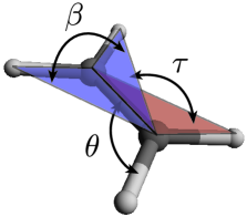
Figure 1: Definition of angular internal coordinates in ethylene.

The ab initio energies were least squares fit to an analytical form consisting of long and short range parts as

$$f=V_{\text{short}}\times f_{\text{damp}}+V_{\text{long}}$$ (1)

where $f_{\text{damp}}$ is a damping function to remove the contribution of the short range component at geometries where the internal coordinates are far from their equilibrium values and has the form

$$f_{\text{damp}}= \exp\left(-\delta_{1}(\xi_{1}^{2}+2\xi_{1}^{4})\right)\times\exp\left(-\delta_{2}\sum_{i=2}^{5}(\xi_{i}^{2}+2\xi_{i}^{4})\right)\times$$ (2)

$$\exp\left(-\delta_{3}\sum_{i=6}^{9}(\xi_{i}^{2}+2\xi_{i}^{4})\right)\times\exp\left(-\delta_{4}\sum_{i=10}^{11}(\xi_{i}^{2}+2\xi_{i}^{4})\right)\times$$ (3)

$$\exp\left(-\delta_{5}(\xi_{12}^{2}+2\xi_{12}^{4})\right).$$ (4)

The damping constants $\delta_{i}$ were kept fixed in the fitting at the values $\delta_{1}=0.3$, $\delta_{2}=0.05$, $\delta_{3}=0.01$, $\delta_{4}=0.005$, $\delta_{5}=0.005$. The long range function has the form

$$V_{\text{long}}= \sum_{i=1}^{5}D^{(2)}_{i}\xi_{i}^{\prime 2}+D^{(4)}_{i}\xi_{i}^{\prime 4}$$ (5)

$$+\exp\left(-\gamma_{1}\xi_{1}^{2}-\gamma_{2}\sum_{i=2}^{5}\xi_{i}^{2}\right)\times\sum_{i=6}^{12}\left(D_{i}^{(2)}\xi_{i}^{2}+D_{i}^{(4)}\xi_{i}^{4}\right),$$

where $\gamma_{1}=0.1$ and $\gamma_{2}=0.1$ and the values for other parameters $D_{i}^{(2)}$ and $D_{i}^{(4)}$ were obtained in the least squares fit to ab initio data points. The short range function is a sum of symmetrised products of form

$$V_{\text{short}}=\sum_{i,j,k,\cdots}\left(\xi_{1}^{\prime i}\,\xi_{2}^{\prime j}\,\xi_{3}^{\prime k}\,\xi_{4}^{\prime l}\,\xi_{5}^{\prime m}\,\xi_{6}^{n}\,\xi_{7}^{o}\,\xi_{8}^{p}\,\xi_{9}^{q}\,\xi_{10}^{r}\,\xi_{11}^{s}\,\xi_{12}^{t}\right)^{\Gamma}C_{ijk\cdots}$$ (6)

where $\Gamma\equiv A_{g}$ produces symmetrized combinations of different permutations of the coordinates in the D_2h(M) molecular symmetry group, $C_{ijk\cdots}$ are expansion parameters, and Morse oscillator functions describe the stretching coordinates $\xi_{i}^{\prime}=1-\exp(-a_{i}\xi_{i})$ with $a_{1}=1.88139$ Å^-1 and $a_{2..5}=1.79890$ Å^-1. The product was limited to a maximum of 8 coordinates coupled at the same time with the sum of powers $i+j+\cdots+t\leq 8$. A total of 1269 terms were used in the sum.

The constants of the long range function in Eq. (5) and the expansion parameters of the short range potential in Eq. (6) were found by least squares fitting to the ab initio energies. Weight factors for energies were used as proposed by Partridge & Schwenke (1997)

$$w_{i}=\left(\frac{{\rm tanh}[-0.0006\times(\tilde{E}_{i}-V_{\rm top})]+1.002002002}{2.002002002}\right)\times\frac{1}{N_{i}{\rm max}(\tilde{E}_{i},V_{\rm lim})},$$ (7)

where $hc\tilde{E}_{i}$ is the electronic energy at $i$-th geometry, $V_{\rm top}=30\,000$ cm^-1, $V_{\rm lim}=15\,000$ cm^-1, and $N_{i}$ is the normalisation constant. A weighted root-mean square (rms) error of 3.2 cm^-1 was obtained for energies up to $hc\cdot 40,000$ cm^-1. Expansion parameters and the explicit forms of the symmetrised products in Eq. (6) are given in a Fortran 90 subroutine in the supplementary information.

To improve the accuracy of nuclear motion calculations, the PES was refined using experimental data. Refinement was carried out using a least-squares fitting procedure as implemented in TROVE (Yurchenko et al., 2011a) with the pruned basis set (see below) in a very similar manner to that described in a recent paper from our group (Owens et al., 2017). Due to the large number of parameters used for the analytical representation of the PES and the size of the eigenfunctions for ethylene, only parameters in Eq. (6) with exponents summing to 2 were allowed to vary. This includes linear ($\xi_{i}$), harmonic ($\xi_{i}^{2}$) and mixed terms ($\xi_{i}\xi_{j}$) for a total of 21 parameters. Refinement was carried out in two stages. First, 109 experimental vibrational $J=0$ band centres taken from Georges et al. (1999) were used. This gave an initial refinement. Then, 21 rotational-vibrational $J=1$ energies from the HITRAN database (Gordon & et al., 2017) were added and the refinement restarted. Pure rotational energies were given the largest weights in the refinement of order 10⁴ followed by $J=1$ rotational-vibrational levels of order 10³ and finally vibrational energies of order 0-10³ depending on the reported accuracy of these levels. Weights are normalised during the refinement and so only relative values are important (Yurchenko et al., 2011a).

The refined PES was found to give accurate values for a further 155 $J=2,3$ and 4 energy levels which were included, but further iterations of refinement did not give improved values. This is due to both the size of the least-squares fitting problem and that added rotational-vibrational levels were from the same vibrational bands as the $J=1$ energies. The difference between all observed energy levels used and the values given by our refined PES is shown in Fig. 2. The vibrational energies with observed$-$calculated errors of $>4$ cm^-1 were retained in the refinement to still provide some constraint to these states but were given relative weightings of a thousand times less than the HITRAN vibrational energies.

For the refined surface we obtained an rms error of 2.73 cm^-1 for the vibrational energies(reduced to 1.95 cm^-1 when bands which were given weights of zero in the refinement were excluded) compared to the values quoted in Georges et al. (1999). This is a large error but many of the bands included also gave large errors for the global effective Hamiltonian model used by Georges et al. and are of low accuracy. Bands with the largest errors were given a weighing of zero in our fit. For the $J=1$ data we obtain an rms error of 0.45 cm^-1 and 0.50 cm^-1 when all $J=1-4$ is included respectively. When combined with the vibrational levels we obtain an overall rms of 1.75 cm^-1, which is reduced to 1.27 cm^-1 when bands which were given weights of zero in the refinement were excluded.

Table 1 compares fundamental vibrational band origins levels with empirical values for both our ab initio and refined PES. The energies were computed variationally using the basis set described in Section 2.3.

Table 1: Comparison of our computed vibrational fundamental band origins for C₂H₄ with the empirical values of Georges et al. (1999). Energies in cm^-1.

Band	Symmetry	Ab initio PES	Refined PES	Obs.a	IRb	TROVEc
$\nu_{1}$	$A_{g}$	3017.951	3021.797	3021.855		$n_{2}+n_{3}+n_{4}+n_{5}=1$
$\nu_{2}$	$A_{g}$	1622.579	1625.648	1625.4		$n_{1}=1$
$\nu_{3}$	$A_{g}$	1341.239	1342.361	1343.54		$n_{6}+n_{7}+n_{8}+n_{9}=1$
$\nu_{4}$	$A_{u}$	1023.089	1024.610	1025.589		$n_{11}+n_{12}=1$
$\nu_{5}$	$B_{3g}$	3078.414	3084.426	3082.36		$n_{2}+n_{3}+n_{4}+n_{5}=1$
$\nu_{6}$	$B_{3g}$	1224.282	1227.050	1222		$n_{6}+n_{7}+n_{8}+n_{9}=1$
$\nu_{7}$	$B_{3u}$	947.846	948.830	948.770	IR	$n_{6}+n_{7}+n_{8}+n_{9}=1$
$\nu_{8}$	$B_{2g}$	937.202	939.069	939.86		$n_{11}+n_{12}=1$
$\nu_{9}$	$B_{2u}$	3100.809	3104.879	3104.872	IR	$n_{2}+n_{3}+n_{4}+n_{5}=1$
$\nu_{10}$	$B_{2u}$	823.402	825.583	825.927	IR	$n_{6}+n_{7}+n_{8}+n_{9}=1$
$\nu_{11}$	$B_{1u}$	2984.018	2988.709	2988.631	IR	$n_{2}+n_{3}+n_{4}+n_{5}=1$
$\nu_{12}$	$B_{1u}$	1438.478	1441.725	1442.475	IR	$n_{6}+n_{7}+n_{8}+n_{9}=1$

^a: Georges et al. (1999)

^b: Infrared active.

^c: Correlation with the local mode (TROVE) quantum numbers.

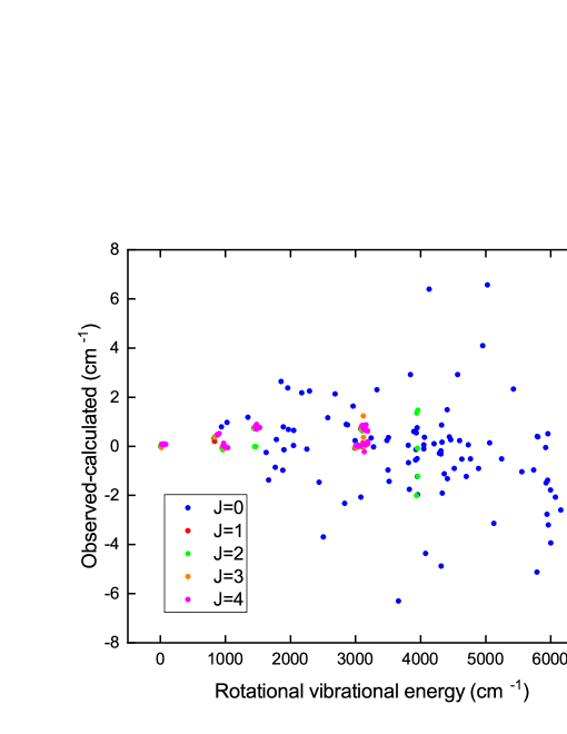
Figure 2: Observed$-$Calculated rotational-vibrational energies after refinement. Vibrational energies (blue dots) with larger discrepancies were given a 1000 times smaller weighting in the refinement with respect to HITRAN vibrational energies.

As is usual for a refined PES used with TROVE (Owens et al., 2017; Underwood et al., 2016a; Al-Refaie et al., 2016; Sousa-Silva et al., 2015; Al-Refaie et al., 2015b; Yurchenko & Tennyson, 2014), the accuracy is only guaranteed with the computational setup employed in this work.

2.2 Dipole Moment Surface

Ab initio calculations for the DMS were carried out at the CCSD(T)-F12b/aug-cc-pVTZ level of theory using the finite field method. The frozen core approximation with a Slater geminal exponent $\beta=1.0$ a${}_{0}^{-1}$ was employed using the same ansatz and auxiliary basis sets as the explicitly correlated PES calculations. For each of the $x$, $y$ and $z$ Cartesian components an electric field of strength $\pm 0.001$ a.u. was applied and the dipole moment projections $\mu_{x}$, $\mu_{y}$ and $\mu_{z}$ computed as derivatives of the electronic energy with respect to the field strength using central finite differences. Calculations were carried out at about 93 000 different molecular geometries with energies up to $hc\cdot 40\,000$ cm^-1, with up to six of the twelve internal coordinates varied at once.

The DMS was fitted to an analytical form as follows. The origin of the molecule-fixed $xyz$ coordinate system ${\bf r}_{O}$ was taken to be the centre of the C₁–C₂ bond. The $z$-axis is chosen to be along the C₁–C₂ bond:

$$\mathbf{e}_{z}=\frac{\mathbf{r}_{{\rm C}_{1}}-{\bf r}_{O}}{||\mathbf{r}_{{\rm C}_{1}}-{\bf r}_{O}||},$$

where $\mathbf{r}_{{\rm C}_{1}}$ denotes Cartesian coordinates of carbon atom C₁. The $x$ axis is a symmetric combination average of the four normals to the four planes C₁C₂H_i ($i=1,2,3,4$) as given by

$$\mathbf{e}_{x}=\frac{\mathbf{e}_{1}+\mathbf{e}_{2}+\mathbf{e}_{3}+\mathbf{e}_{4}}{||\mathbf{e}_{1}+\mathbf{e}_{2}+\mathbf{e}_{3}+\mathbf{e}_{4}||}$$

and the $y$ axis is chosen as in the right-handed system. Here the normals are defined using the cross-products of the unit vector $\mathbf{e}_{z}$ with the corresponding C–H bond vectors $\mathbf{e}_{{\rm H}_{i}}=(\mathbf{r}_{{\rm H}_{i}}-{\bf r}_{O})/||\mathbf{r}_{{\rm H}_{i}}-{\bf r}_{O}||$ ($i=1..4$) as given by

$$\mathbf{e}_{1}=-\frac{\mathbf{e}_{z}\times\mathbf{e}_{{\rm H}_{1}}}{||\mathbf{e}_{z}\times\mathbf{e}_{{\rm H}_{1}}||}, \quad\mathbf{e}_{2}=\frac{\mathbf{e}_{z}\times\mathbf{e}_{{\rm H}_{2}}}{||\mathbf{e}_{z}\times\mathbf{e}_{{\rm H}_{2}}||},$$

$$\mathbf{e}_{3}=-\frac{\mathbf{e}_{z}\times\mathbf{e}_{{\rm H}_{3}}}{||\mathbf{e}_{z}\times\mathbf{e}_{{\rm H}_{3}}||}, \quad\mathbf{e}_{4}=\frac{\mathbf{e}_{z}\times\mathbf{e}_{{\rm H}_{4}}}{||\mathbf{e}_{z}\times\mathbf{e}_{{\rm H}_{4}}||},$$

where $\mathbf{r}_{{\rm H}_{i}}$ denotes Cartesian coordinates of hydrogen atoms. The Cartesian axes $x$, $y$ and $z$ transform according to D_2h(M) as $B_{3u}$, $B_{2u}$ and $B_{1u}$ irreducible representations (irreps), respectively.

The dipole moment vector can be expressed as

$${\boldsymbol{\mu}}=\mu_{x}\mathbf{e}_{x}+\mu_{y}\mathbf{e}_{y}+\mu_{z}\mathbf{e}_{z},$$ (8)

where $\mu_{\alpha}$ ($\alpha=x,y,z$) are functions of the internal coordinates of the form

$$\mu_{\alpha}=\sum_{i,j,k,\cdots}\left(\xi_{1}^{i}\,\xi_{2}^{j}\,\xi_{3}^{k}\,\cdots\xi_{12}^{t}\right)^{\Gamma}F^{(\alpha)}_{ijk\cdots}$$ (9)

where $\Gamma$ produces symmetrized combinations of different permutations of the coordinates in the $B_{3u}$, $B_{2u}$ and $B_{1u}$ irreps for $\alpha=x$, $y$ and $z$, respectively, and $F^{(\alpha)}_{ijk\cdots}$ are the expansion parameters. The symmetry-adapted analytical expressions in Eq. (9) have been obtained using the SymPy Python library for symbolic mathematics (Meurer et al., 2017). The Python program is freely available from the authors upon request. The coordinates $\xi_{1},\xi_{2},...\xi_{12}$ chosen for analytical representation of the DMS in Eq. (9) are the same as those used for the PES.

For each component of the dipole we used a sixth-order expansion consisting of 1881, 1861 and 1399 terms for the $B_{1u}$, $B_{2u}$ and $B_{3u}$ symmetries, respectively. The expansion parameters $F^{(\alpha)}_{ijk\cdots}$ were determined by least squares fitting to the ab initio data giving rms errors of $7\times 10^{-4}$, $7\times 10^{-4}$ and $6\times 10^{-4}$ D, respectively. The expansion parameters $F^{(\alpha)}_{ijk\cdots}$ and Fortran 90 subroutines to compute $\mu_{\alpha}$ are provided as part of the supplementary information.

2.3 Variational Calculations

Variational ro-vibrational calculations were carried out using the TROVE program. The TROVE methodology is well documented (Yurchenko et al., 2007; Yurchenko et al., 2009; Yachmenev & Yurchenko, 2015; Yurchenko et al., 2017a; Tennyson & Yurchenko, 2017) and has been applied to a variety of molecules as part of the ExoMol project (Yurchenko et al., 2009; Yurchenko et al., 2011b; Sousa-Silva et al., 2013; Polyansky et al., 2013; Underwood et al., 2013; Yurchenko & Tennyson, 2014; Sousa-Silva et al., 2015; Al-Refaie et al., 2015b, a; Owens et al., 2015; Underwood et al., 2016b; Owens et al., 2017). Only the specific details used in this work on ethylene will be discussed here.

The ro-vibrational Hamiltonian was constructed numerically via an automatic differentiation method (Yachmenev & Yurchenko, 2015). The Hamiltonian was expanded using a power series in curvilinear coordinates around the equilibrium geometry of the molecule. The coordinates used were the same as those used to fit the PES.

The kinetic energy operator was expanded to the 6th order and the potential energy operator to the 8th order. The same Morse coordinates as used in Eq. (6) were used for the potential expansion for the stretching coordinates ($i=1-5$) with the other bending coordinates expanded as $\xi_{i}$ themselves. Atomic masses were used throughout.

A multistep contraction scheme was used to build the vibrational basis set. For each coordinate a one-dimensional Schrödinger equation was solved using the Numerov-Cooley approach (Noumerov, 1924; Cooley, 1961; Yurchenko et al., 2007) to generate basis functions $\phi_{n_{i}}(\xi_{i})$ with vibrational quantum number $n_{i}$. The vibrational basis set functions $|v\rangle$ are formed as products of the 1D basis functions

$$|v\rangle=\prod_{\nu}|n_{\nu}\rangle=\phi_{n_{1}}(\xi_{1})\phi_{n_{2}}(\xi_{2})\ldots\phi_{n_{12}}(\xi_{12}).$$ (10)

The basis set is truncated by the polyad number $P$ via

$$P=n_{1}+2(n_{2}+n_{3}+n_{4}+n_{5})+n_{6}+n_{7}+n_{8}+n_{9}+n_{10}+n_{11}+n_{12}\leq P_{\text{max}}.$$ (11)

A value of $P_{\text{max}}=10$ was used. This is a smaller value than used for previous Exomol line lists (Underwood et al., 2016a; Sousa-Silva et al., 2015; Owens et al., 2017; Yurchenko & Tennyson, 2014; Al-Refaie et al., 2016, 2015b) but with 12 degrees-of-freedom the basis set rapidly increases with increasing $P$. To estimate the converge of vibrational energies with this basis set we used a complete vibrational basis set (CVBS) extrapolation procedure similar to that described by Owens et al. (2015). Variational calculations were carried out with $P_{\text{max}}=6,8$ and 10 respectively. From this we estimate that above 4000 cm^-1 there are some vibrational levels (typically those with multiple bending modes excited) which are only converged to around 4 cm^-1 with a $P_{\text{max}}=10$ basis. The average convergence error for 0–5 000 cm^-1 is estimated to be only 1.5 cm^-1 however. It should be noted that these estimates do not account for the fact that the PES refinement procedure described above tends to compensate partly or fully for the basis set convergence errors, even when extrapolating to higher vibrational excitations. Strictly speaking, in order to get a sensible convergence error, one would need to produce a refined PES for all three values of $P_{\text{max}}=6,8$ and 10. These estimates do however indicate the possible error of our effective ($P=10$) PES if used with larger basis sets or other nuclear motion methods.

To extend the vibrational basis, further 1D and 2D functions were added with $\phi_{n_{i}}(\xi_{i})$ ($n=11,12,13,14$) and $\phi_{n_{i}}(\xi_{i})\phi_{n_{j}}(\xi_{j})$ ($10\leq i+j\leq 14$). A contracted basis set was then formed by reducing the 12 dimensional problem into 5 subspaces: ($\xi_{1}$), ($\xi_{2},\xi_{3},\xi_{4},\xi_{5}$), ($\xi_{6},\xi_{7},\xi_{8},\xi_{9}$), ($\xi_{10},\xi_{11}$) and ($\xi_{12}$). A Hamiltonian matrix is constructed and diagonalised for each of these subspaces to give symmetrised contracted vibrational basis functions. The details of this step have been discussed in a recent publication (Yurchenko et al., 2017a). Products of these eigenfunctions are formed which are also truncated via Eq. (11).

To increase the computational efficiency of this step, a new algorithm for sorting and calculating matrix elements of the PES between primitive basis functions was implemented. This procedure also sets these elements to zero for potential expansion coefficients with values smaller than a tolerance factor. Here we take this as 0.01 (in the units of cm^-1, Angstrom and radian). This procedure led to around a 70 fold speed up for smaller basis test calculations whilst only affecting the accuracy of vibrational states by 0.01 cm^-1, far lower than the error of the ab initio PES. This new ‘fast-ci’ method will be described fully in a subsequent publication.

Following this procedure, 145 240 vibrational eigenfunctions $|\Phi_{\text{vib}}^{(i)}\rangle$ of C₂H₄ were obtained with term energies $\tilde{E}_{i}^{(J=0)}$ up to 21 000 cm^-1 above the ground state (our post refinement zero-point-energy is 11 022.5 cm^-1). According to the $J=0$-contraction scheme TROVE uses these $J=0$ eigenfunctions as the vibrational basis set. However using a basis set of this size for high rotationally excited levels is currently impractical and it was necessary to reduce the number of basis functions. The basis set was further truncated using the same approach based on the vibrational band intensity as described in a recent paper for the silane (SiH₄) line list (Owens et al., 2017), which will be referenced to as intensity basis set pruning (IBSP). According to this approach, the vibrational basis functions $|\Phi_{\text{vib}}^{(i)}\rangle$ above some energy threshold, $\tilde{E}_{\rm max}^{(J=0)}$, should be truncated with the exception of functions responsible for significant contribution to the absorption opacity (larger than some intensity threshold $I_{\rm max}$). In turn, the absorption contribution is estimated from the intensities of the corresponding bands using these functions as the upper or lower states.

We define the vibrational absorption intensity (cm$/$molecule) for the band $f\leftarrow i$ as

$$I_{fi}^{(J=0)}=\frac{A_{fi}^{(J=0)}}{8\pi c}\frac{\exp(-c_{2}\tilde{E}_{i}^{(J=0)}/T)}{Q^{(J=0)}\left(\tilde{\nu}^{(J=0)}_{fi}\right)^{2}}.$$ (12)

The vibrational Einstein coefficient (s^-1) is given by

$$A_{fi}^{(J=0)}=\frac{8\times 10^{-36}\pi^{4}\left(\nu^{(J=0)}_{fi}\right)^{3}}{3h}\bar{\mu}_{fi}^{2},$$ (13)

where the vibrational transition moment $\mu_{fi}$ (D) is

$$\bar{\mu}_{fi}=\sqrt{\sum_{\alpha=x,y,z}\left|\langle\Phi_{\text{vib}}^{f}|\bar{\mu}_{\alpha}|\Phi_{\text{vib}}^{i}\rangle\right|^{2}}.$$ (14)

Here $h$ is Planck’s constant, $Q^{(J=0)}$ is the vibrational ($J=0$) partition function, $\tilde{E}_{i}^{(J=0)}$ and $\tilde{\nu}_{fi}^{(J=0)}$ are the vibrational lower state term value and band centres, respectively and $c_{2}$ is the second radiation constant. Here $|\Phi_{\text{vib}}^{(i)}\rangle$ and $\langle\Phi_{\text{vib}}^{(f)}|$ are the initial and final state vibrational eigenfunctions, respectively and $\bar{\mu}_{\alpha}$ is the electronically averaged dipole moment along the molecular fixed axis $\alpha=x,y,z$.

The vibrational absorption intensities were computed between each state at an elevated temperature of 800 K. For each vibrational state, the largest intensity to or from that state was then associated with that state. The $J=0$ basis set was then pruned based on this. All states up to $hc\cdot$8000 cm^-1 were retained. States with energy above this were discarded if their largest intensity was less than some value $I_{\text{max}}$. Here a value of $I_{\text{max}}=1\times 10^{-24}$ cm$/$molecule was used. This value was chosen to retain as many states as possible (which support intense transitions) whilst making the calculations for high $J$ practical. The resulting pruned vibrational basis contained 13 572 functions corresponding to energies up to $hc\cdot 12~{}000$ cm^-1. This basis was then used for $J>0$ calculations by combining it with symmetrized rigid-rotor functions as described previously (Yurchenko et al., 2009, 2017a).

The pruning procedure based on the $J$=$0$-contraction has the advantages that the accuracy of the vibrational energy levels and eigenfunctions computed using the unpruned basis is retained. The errors introduced in pruning the basis for the ro-vibrational levels are compensated for by refining the PES with the pruned basis.

Fig. 3 shows vibrational intensities of C₂H₄ computed using Eq. (12) for $T=500$ K as cross sections. Here we compare the total cross sections (no pruning) and the contribution missing due to the intensity-based pruning. The effect of the pruning on the intensities is negligible for the range below 7000 cm^-1 ($\sim$ 0.01 %). This is especially important for hot spectra applications, where the completeness of the molecular absorption arguably plays a more important role than the accuracy (Yurchenko et al., 2014).

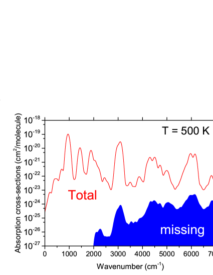
Figure 3: The vibrational cross sections: total compared to the missing contribution due to the vibrational pruning.

A final empirical basis set correction was also made to shift vibrational band centres to experimental values. As the $J=0$ basis is diagonal with respect to the vibrational component of the Hamiltonian, experimental band centres can be used instead (Yurchenko et al., 2011a). This was carried out for bands with observable Q branches namely: the $\nu_{12}$ band at 1442.4750 cm^-1 (Rusinek et al., 1998), the $\nu_{2}+\nu_{12}$ band at 3078.46270 cm^-1 (Rusinek et al., 1998), $\nu_{7}+\nu_{8}$ band at 1888.9748 cm^-1 (Rusinek et al., 1998), $\nu_{6}+\nu_{10}$ band at 2047.76 cm^-1 (Rusinek et al., 1998) and $\nu_{5}+\nu_{9}$ band at 6150.98104 cm^-1 (Bach et al., 1999).

For ro-vibrational states with $0\leq J\leq 24$, variational calculations were carried out using TROVE in a standard manner. That is, the Hamiltonian was constructed and diagonalised with all data kept in RAM memory. The largest matrix to be diagonalised in this case had around 82 000 rows per symmetry for $J=24$. For states with $J>24$ however, this was not possible. Instead the procedure described by Underwood et al. (2016b) for the SO₃ line list was used. This involved first calculating the Hamiltonian and then saving to disk. Diagonalisation was then carried out using an MPI-optimized version of the eigensolver, PDSYEVD. This was carried out separately for each $J$ and symmetry $\Gamma$, where $\Gamma$= $A_{1g},A_{1u},B_{1g},B_{1u},B_{2g},B_{2u},B_{3g}$ and $B_{3u}$. A final run of TROVE is required to reformat the eigenvalues and eigenvectors into the proper format. The largest matrix diagonalised had 150 000 rows for $J=50$. For $J>50$ the Hamiltonian decreases in size as we only retain eigenvalues less than 18 000 cm^-1.

2.4 Line Intensities

The eigenvectors from the variational calculation along with the DMS were used to compute Einstein-A coefficients of transitions. These satisfy the rotational selection rules (Bunker & Jensen, 1998)

$$J^{\prime}-J^{\prime\prime}=0,\pm 1,\quad{\rm and}\quad J^{\prime}+J^{\prime\prime}\neq 0,$$ (15)

where $J^{\prime}$ and $J^{\prime\prime}$ are the upper and lower values of the total angular quantum number $J$ and symmetry selection rules

$$A_{1g}\leftrightarrow A_{1u},B_{1g}\leftrightarrow B_{1u},B_{2g}\leftrightarrow B_{2u},B_{3g}\leftrightarrow B_{3u}.$$ (16)

The absolute absorption intensities are then given by (Bunker & Jensen, 1998)

$$I(f\leftarrow i)=\frac{A_{fi}}{8\pi c}g_{ns}(2J_{f}+1)\frac{\exp(-c_{2}\tilde{E}_{i}/T)}{Q(T)\tilde{\nu}^{2}_{fi}}\times\left[1-\exp\left(-\frac{c_{2}\tilde{\nu}_{fi}}{T}\right)\right],$$ (17)

where $J_{f}$ is the rotation quantum number for the final state, $\tilde{\nu}_{fi}$ is the transition frequency ($\tilde{\nu}_{fi}=\tilde{E}_{f}-\tilde{E}_{i}$), $\tilde{E}_{i}$ and $\tilde{E}_{f}$ are the initial and upper state term values, respectively, and $Q(T)$ is the partition function (Section 3.1). The Einstein-A coefficients $A_{fi}$ between the ro-vibrational states $i$ and $f$ are defined in Yurchenko et al. (2005). The nuclear spin statistical weights $g_{ns}$ for ethylene are (7,7,3,3,3,3,3,3) for states of symmetry ($A_{1g},A_{1u},B_{1g},B_{1u},B_{2g},B_{2u},B_{3g},B_{3u}$) respectively (Bunker & Jensen, 1998) within the HITRAN convention, adopted by ExoMol, of including the full nuclear spin of each species.

The temperature independent Einstein-A coefficients were computed using the GAIN-MPI program (Al-Refaie et al., 2017). With this program we were able to calculate up to 93 000 transitions per second using NVIDIA Tesla P100 GPUs on the Wilkes2 cluster.

Intensities were computed using a lower energy range of 0 – 5000 cm^-1 taking into account up to $J=78$ for transitions frequencies between 0 and 7000 cm^-1. An intensity cut-off of 10^-50 cm molecule^-1 at $T=298$ K was used, ensuring that essentially all transitions are taken into account for up to around 700 K (see section 3.1).

3 Results

3.1 Partition Function

The temperature-dependent partition function $Q(T)$ is defined as

$$Q(T)=\sum_{i}g_{i}\exp\left(-c_{2}\frac{\tilde{E}_{i}}{T}\right),$$ (18)

where $g_{i}=g_{ns}(2J_{i}+1)$ is the degeneracy of the state $i$ with energy $E_{i}$ and rotational quantum number $J_{i}$.

Fig. 4 shows the convergence of $Q(T)$ as a function of $J$ at different temperatures. At 700 K the partition function is converged to 0.02%. In Table 2 we compare the partition function calculated at various temperature with those of literature values. In general agreement between the various sources is good. Our value which increases slightly faster with temperature than those of Rey et al. (2016) is probably due to our more complete treatment of the energy levels. In the supplementary information we provide the partition function between 0 and 1500 K at 1 K intervals.

The current line list was computed with a lower energy threshold of $hc\cdot 5000$ cm^-1. To assess the completeness of our line list we compute a reduced partition function, $Q_{\text{limit}}$ which only takes into account energies up to $hc\cdot 5000$ cm^-1 in Eq. (18). Fig. 4 also shows a plot of the ratio of $Q_{\text{limit}}/Q$. At 700 K the ratio is 0.98 and this temperature can be taken as a soft limit. At higher temperatures opacity will progressively be underestimated (see Section 4).

Table 2: Comparison of partition functions with literature values.

$T$(K)	Refs	$Q_{\text{vib}}$	$Q_{\text{rot}}$	$Q_{\text{vib}}Q_{\text{rot}}$	Direct Sum
80	This work	1	1472.7	1472.7	1479.7
	Blass et al. (2001)	1	1467.9	1467.9
	Gamache et al. (2017)			1474.2
	Rey et al. (2016)	1	1471.7	1471.7	1471.7
160	This work	1.0011	4169.6	4174.4	4181.4
	Blass et al. (2001)	1.0009	4143.3	4147.1
	Gamache et al. (2017)			4169.4
	Rey et al. (2016)	1.0011	4154.0	4158.6	4158.8
296	This work	1.0522	10498.3	11046.3	11058.6
	Blass et al. (2001)	1.0469	10421.4	10910.1
	Gamache et al. (2017)			11041.5
	Carter et al. (2012)				10979.2 ($J<40$)
	Rotger et al. (2008)	1.0469	10432.9	10922.2
	Rey et al. (2016)	1.0521	10448.4	10992.8	10997.8
500	This work	1.4402	23069.5	33224.8	33306.1
	Gamache et al. (2017)			33271.3
	Rey et al. (2016)	1.4396	22951.3	33040.7	33117.2
700	This work	2.4298	38251.5	92942.0	93373.4
	Gamache et al. (2017)			93244.0
	Rey et al. (2016)	2.4274	38048.0	92357.7	92702.8

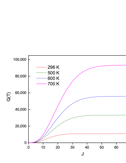
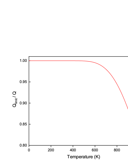
Figure 4: Partition functions of C₂H₄: Convergence of partition function $Q(T)$ at different temperatures with respect to the rotational quantum number $J$ (left) and $Q_{\text{limit}}/Q$ as a function of temperature (right).

3.2 Line List Format

A complete description of the ExoMol data structure along with examples was reported by Tennyson et al. (2016). The .states file contains all computed ro-vibrational energies (in cm^-1) relative to the ground state. Each energy level is assigned a unique state ID with symmetry and quantum number labelling as shown in Table 4. The .trans files, which are split into frequency windows for ease of use, contain all computed transitions with upper and lower state ID labels, and Einstein A coefficients. An example from a .trans file for the line list is given in Table 4.

Table 3: Extract from .states file for MaYTY line list.

$N$	$\tilde{E}$	$g_{\text{tot}}$	$J$	$\Gamma_{\text{tot}}$	$n_{1}$	$n_{2}$	$n_{3}$	$n_{4}$	$n_{5}$	$n_{6}$	$n_{7}$	$n_{8}$	$n_{9}$	$n_{10}$	$n_{11}$	$n_{12}$	$\Gamma_{\text{vib}}$	$J$	$K$	$\tau_{\text{rot}}$	$\Gamma_{\text{rot}}$
1	0.000000	7	0	1	0	0	0	0	0	0	0	0	0	0	0	0	1	0	0	0	1
2	1342.361058	7	0	1	0	0	0	0	0	1	0	0	0	0	0	0	1	0	0	0	1
3	1625.647919	7	0	1	1	0	0	0	0	0	0	0	0	0	0	0	1	0	0	0	1
4	1663.565812	7	0	1	0	0	0	0	0	1	0	1	0	0	0	0	1	0	0	0	1
5	1881.875767	7	0	1	0	0	0	0	0	0	0	0	0	0	2	0	1	0	0	0	1
6	1899.881666	7	0	1	0	0	0	0	0	0	0	0	0	1	1	0	1	0	0	0	1
7	2046.368511	7	0	1	0	0	0	0	0	0	0	0	0	0	0	2	1	0	0	0	1
8	2452.971198	7	0	1	0	0	0	0	0	1	0	0	1	0	0	0	1	0	0	0	1
9	2683.172133	7	0	1	1	0	0	0	0	1	0	0	0	0	0	0	1	0	0	0	1
10	2784.166877	7	0	1	0	0	0	0	0	0	0	1	0	0	1	1	1	0	0	0	1

$N$ : State ID;

$\tilde{E}$: Term value (in cm^-1);

$g_{\text{tot}}$: Total degeneracy;

$J$: Total angular momentum;

$\Gamma_{\text{tot}}$: Total symmetry in D_2h(M) (1 is $A_{g}$, 2 is $A_{u}$, 3 is $B_{1g}$, 4 is $B_{1u}$, 5 is $B_{2g}$, 6 is $B_{2u}$, 7 is $B_{3g}$ and 8 is $B_{3u}$);

$n_{1}$-$n_{12}$: TROVE vibrational quantum numbers (QN); see Table 1 for the correlation with the normal QNs;

$\Gamma_{\text{vib}}$: Symmetry of vibrational component of state in D_2h(M);

$K$: Projection of $J$ on molecule-fixed $z$-axis;

$\tau_{\text{rot}}$: Rotational parity (0 or 1);

$\Gamma_{\text{rot}}$: Symmetry of rotational component of state in D_2h(M).

Table 4: Extract from .trans file for MaYTY line list.

$f$	$i$	$A_{fi}$
49589	44178	2.4146E-07
49590	44178	2.1037E-05
12140	44178	2.1033E-05
49591	44178	1.8719E-05

$f$: Upper state ID;

$i$: Lower state ID;

$A_{fi}$: Einstein A coefficient (in s^-1).

3.3 Validation

The MaYTY line list contains nearly 50 billion (49 841 085 051) transitions between over 45 million (45 446 267) states.

Fig. 5 and 6 compare the MaYTY line list to empirical intensities from the HITRAN database at 296 K. To take into account the abundance of the ¹²C₂¹H₄ isotopologue we divide the HITRAN intensities by 0.97729 to obtain the value for pure ¹²C₂¹H₄. Fig. 5 gives an overview of our line list compared to HITRAN. HITRAN is currently missing data for the 1600 – 2750 cm^-1 region which contains the relatively intense $\nu_{7}+\nu_{8}$ band amongst others. For this region Fig. 6 compares our line list to that of Rey et al. (2016) from the TheoReTS database. HITRAN also currently does not have any data above 3500 cm^-1.

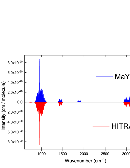
Figure 5: Overview of absolute intensities of MaYTY compared to HITRAN data at 296 K.

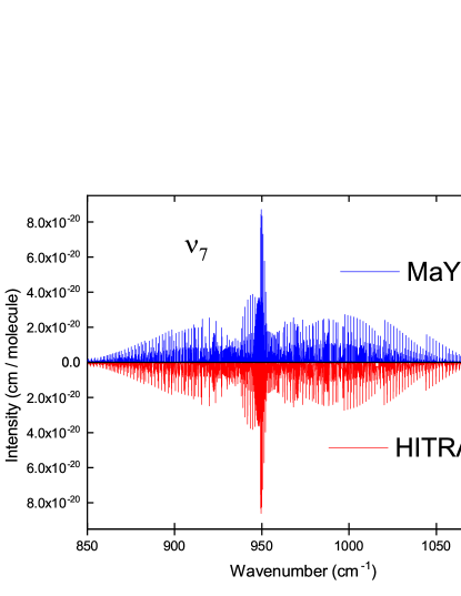
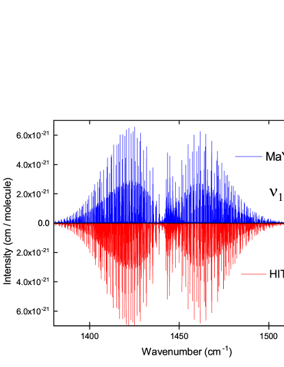
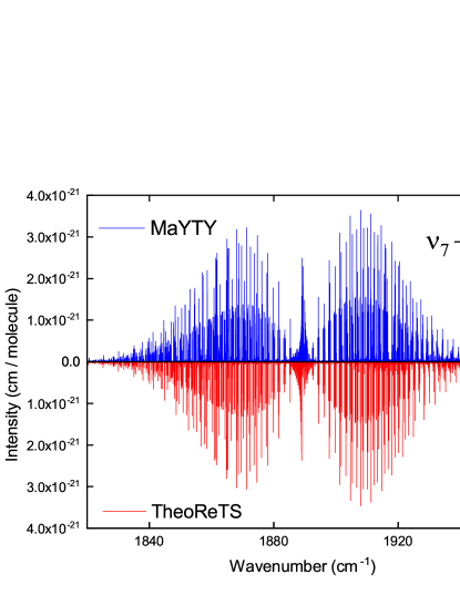
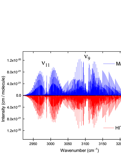
Figure 6: Detailed comparison of the MaYTY line list those from HITRAN and TheoReTS at 296 K. The strongest bands are labelled in each plot.

As a further comparison of the MaYTY line list to experiment we compare cross sections to those in the PNNL database (Sharpe et al., 2004) in Fig. 7. The PNNL spectrum is a composite recorded at 298 K and re-normalized for 296 K. The ethylene used was 99.5 % pure. For comparison with our line list PNNL cross sections were multiplied by $9.28697\times 10^{-16}$/0.97729 to convert to cm² molecule^-1 units and account for the ¹²C₂¹H₄ isotopologue. We simulated the spectrum using a resolution of 0.1 cm^-1 using a Voigt profile with a half-width half-maximum (HWHM) value of 0.1 cm^-1. The PNNL spectrum allows a comparison to our calculated line list up to around 6200 cm^-1.

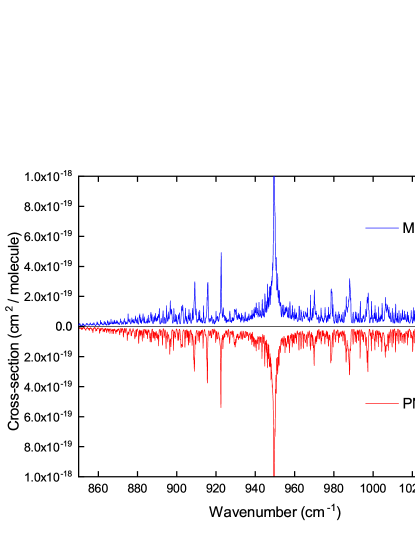
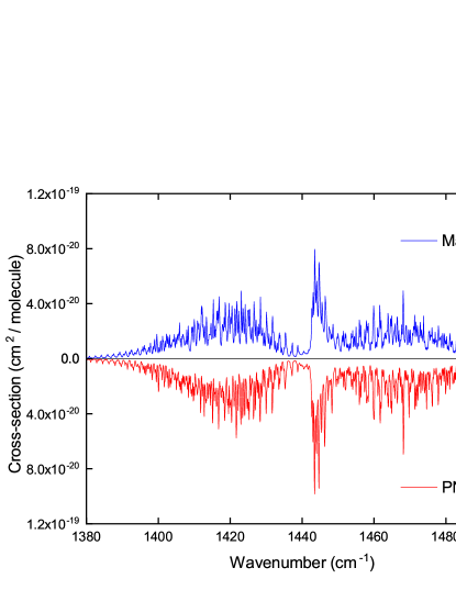
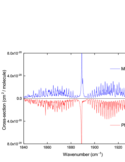
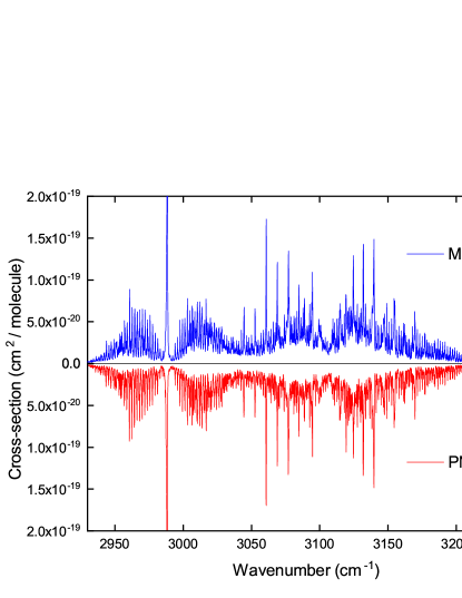
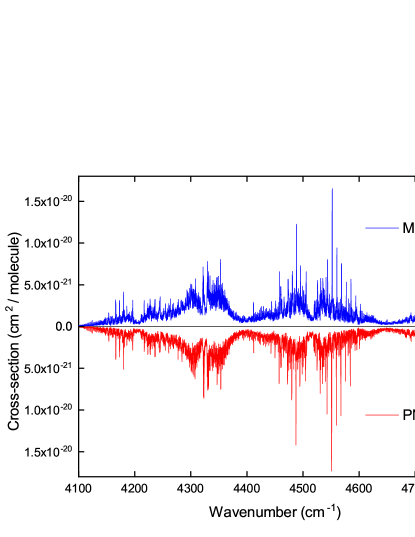
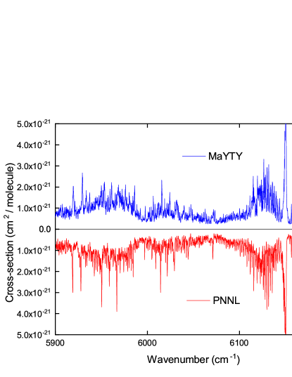
Figure 7: Comparisons of MaYTY line list to PNNL cross sections at 296 K

Fig. 8 shows the temperature dependence of the absorption cross sections for the MaYTY line list simulated using a resolution of 5 cm^-1 where again a Voigt profile with a HWHM of 0.1 cm^-1 was used. While regions of weak absorption at 296 K increase by an order of magnitude or more as the temperature is increased, the overall band structure of the absorption does not change greatly with temperature. This behaviour contrasts with other molecules, such as methane (Yurchenko & Tennyson, 2014), whose band shapes show a strong temperature dependence.

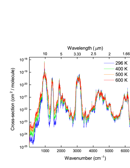
Figure 8: Infrared absorption spectrum of ¹²C₂¹H₄: Temperature dependence of MaYTY line list.

4 Vibrational cross sections: realistic band shapes

Our final ro-vibrational line list for C₂H₄ is limited to the frequency range of 0 – 7 000 cm^-1 and the temperatures up to about 700 K. On the other hand, our vibrational line list, which we used to assist the basis set pruning, has much larger coverage, both in terms of frequency and temperature ranges. Here we show how to use this more complete vibrational line list to (i) top-up the ro-vibrational line list with missing opacities and (ii) directly simulate realistic spectra at high temperatures for large polyatomic molecules.

The vibrational line list consists of the vibrational Einstein coefficients $A_{fi}^{(J=0)}$ generated using Eq. (13), which are stored using the ExoMol line list format: the vibrational .trans has the same format as in Table 5, i.e. with the upper state ID, lower state ID and the third column containing $A_{fi}^{(J=0)}$. The vibrational .states file contains all the vibrational energy term values labelled with their IDs, as in Table 3; the only difference with the ro-vibrational .states file is that the statistical weights are all set to 1 according with Eqs. (12) and (13). The vibrational line list in this format can be used together with ExoCross to generate absorption vibrational intensities using Eq. (12) (instead of its ro-vibrational analogy in Eq. (17)). Another potential application of our extensive vibrational line list for ethylene is to generate spectra using the spectroscopic tool PGOPHER (Western, 2017). One of the recent features of PGOPHER is to import band centers and and transition moments from an external vibrational line list.

Here we use the hot vibrational line list for C₂H₄ to produce temperature-dependent vibrational cross sections by ‘broadening’ the corresponding band intensity with suitable band profiles. The vibrational cross sections should, at least approximately, conserve the opacity stored in each vibrational band and thus offer an approximate but simple way of simulating molecular opacity.

In fact, it is common in applications involving large polyatomic molecules to use vibrational intensities for modelling molecular absorption, where Lorentzian or Gaussian functions are used as band profiles. There are also more realistic but elaborate alternatives to represent the band profiles, such as, for example the narrow band approach (Consalvi & Liu, 2015). Here we develop a three-band model, where different vibrational bands (perpendicular and parallel) are modelled using three realistic basic shapes, corresponding to three components of the vibrational dipole moment $\bar{\mu}_{\alpha}$ of ethylene.

Table 5: Extract from vibrational .trans file.

$f$	$i$	$\mu_{fi}$
65040	1	5.44101247E-07
1040	1	3.33556008E-16
85543	1	1.81580111E-16
127077	1	7.88402351E-16
63744	1	1.92578661E-07
8779	1	1.45418720E-16
43097	1	1.23733815E-20

$f$: Upper state ID;
$i$: Lower state ID;
$\mu_{fi}$: Vibrational transition moment (in D).

As indicated in Table 1, only the $\nu_{7}$, $\nu_{9}$, $\nu_{10}$, $\nu_{11}$, $\nu_{12}$ bands are IR active: $\nu_{9}$ and $\nu_{10}$ (see Figs. 6) are parallel bands as they possess the same symmetry $B_{1u}$ as the $z$ component of the molecular dipole moment $\boldsymbol{\mu}$. The perpendicular bands $\nu_{11}$ and $\nu_{12}$ are of the type $B_{2u}$ (corresponding to $\bar{\mu}_{y}$), while the perpendicular band $\nu_{7}$ is of the type $B_{3u}$ ($\mu_{x}$). These three band types ($B_{1u}$, $B_{2u}$ and $B_{3u}$) have different shapes, which we use as templates to model all other vibrational bands of C₂H₄. We select the three strongest fundamental bands, one for each type: $\nu_{12}$ ($B_{1u}$), $\nu_{9}$ ($B_{2u}$) and $\nu_{7}$ ($B_{3u}$), and use the corresponding ro-vibrational cross sections at different temperatures to construct three temperature-dependent, normalised band profiles as follows. For each temperature and band in question the corresponding cross-sections on a grid of 1 cm^-1 are normalised and shifted to have the center at $\tilde{\nu}=0$. Three profile templates for $T=500$ K and $T=1500~{}K$ are shown in Fig. 9. The $T=500$ K profiles were generated using the MaYTY line list in conjunction with the Voigt line profile with HWHM=0.1 cm^-1. For the $1500$ K temperature case our line list is rotationally incomplete ($J_{max}=78$), therefore we used the effective Hamiltonian approach to generate the corresponding band profiles with significantly higher $J_{\rm max}=120$. Towards this we employed PGOPHER together with the $\nu_{7}$, $\nu_{9}$ and $\nu_{12}$ spectroscopic constants from Bach et al. (1998) and Rusinek et al. (1998), and a Voigt line profile with HWHM=0.1 cm^-1.

These profiles are then applied for the vibrational cross sections at the temperature in question by using the symmetry multiplication rule: if $\Gamma_{i}$ and $\Gamma_{f}$ are, respectively, the symmetries of the initial and upper states and $\Gamma_{\alpha}$ is the symmetry of the dipole moment component $\bar{\mu}_{\alpha}$, for an IR active band $\tilde{\nu}_{fi}^{(J=0)}$ the following relation holds (Bunker & Jensen, 1998):

$$\Gamma_{\alpha}=\Gamma_{i}\otimes\Gamma_{f}.$$

Note that the equal sign here (not $\in$) is due to D_2h(M) being an Abelian symmetry group. We thus use this rule to choose between the $B_{1u}$, $B_{2u}$ or $B_{3u}$ templates when generating cross sections for specific bands $\tilde{\nu}_{fi}^{(J=0)}$. This rule, however, does not always hold: a large number of forbidden (and weak) bands have non-zero intensities due to interactions between vibrational states. In such cases we use a simple Lorentzian band profile with HWHM of 60 cm^-1.

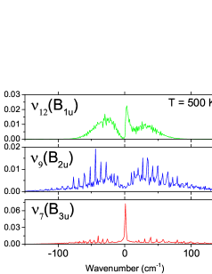
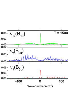
Figure 9: Normalized $\nu_{12}$, $\nu_{9}$ and $\nu_{7}$ band profiles with a HWHM=0.1 cm^-1. Left: the $T=500$ K profiles were generated using the MaYTY line list with the Voigt profile. Right: The $T=1500$ K profile was generated using PGOPHER with the Lorentzian line broadening and spectroscopic constants from Bach et al. (1998) and Rusinek et al. (1998).

An example of vibrational cross sections of C₂H₄ at $T=500$ K and $T=1500$ K generated using this methodology is shown in Fig. 10, where they are also compared to the ro-vibrational cross sections. The vibrational cross sections are more complete and also provide larger coverage (here shown up to 10 000 cm^-1). For example, the lower display on Fig. 10 shows the predicted opacity of C₂H₄ at $T=1500$ K by using our vibrational cross section technique compared to the MaYTY intensities, which are incomplete at $T=1500$ K.

The methodology of combining realistic band profiles with vibrational intensities can be especially useful for larger polyatomic molecules, where the size of the calculations becomes prohibitive. This requires knowing the ro-vibrational spectra of the three fundamental bands to generate the realistic band profiles, for which we took advantage of having the complete, ro-vibrational line list. In practical applications when this is not accessible, these profiles could be modelled using effective rotational methods, using for example PGOPHER (Western, 2017) as we demonstrated , which only requires the corresponding spectroscopic constants of these (up to) three fundamental bands.

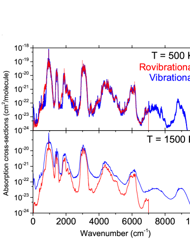
Figure 10: Comparing the ro-vibrational and vibrational intensities of C₂H₄ at $T=500$ K and $T=1500$ K: The ‘ro-vibrational’ cross sections of C₂H₄ were computed using the MaYTY line list and the Gaussian line profile with HWHM=1 cm^-1. The ‘vibrational’ cross sections were computed using the vibrational line list with the normalized band profiles scheme (see text).

The temperature dependent vibrational cross sections can be useful for evaluating opacities of molecules (especially at higher temperatures) when completeness is more important than high accuracy. The approximations used for vibrational intensities are: (i) the rotational and vibrational degrees of freedom are independent and (ii) lower resolution is assumed.

Due to the missing interaction between the rotational and vibrational degrees of freedom, this vibrational methodology is not capable of reconstructing some forbidden bands, which are caused by this interaction. This is evident in Fig. 10, where some weaker parts are missing. It is important to note that the vibrational band intensity of a given vibrational band computed using Eq. (12) is the same as the corresponding integrated ro-vibrational intensities from Eq. (17), at least if the interaction with other vibrational bands is ignored. Thus although the vibrational intensity treatment is highly approximate, it should be better for preserving the opacity in simulations.

In line with our ‘hybrid’-methodology (Yurchenko et al., 2017b), the generated vibrational cross sections can be now divided into the strong and weak parts, with the latter representing the absorption, missing from our line list due to the vibrational basis set pruning. These ‘weak’ vibrational bands form absorption ‘continuum’ cross sections and can be used to compensate for missing absorption when higher temperatures or larger spectroscopic coverage is required. Fig. 11 shows this absorption continuum of C₂H₄ at $T=500$ K up to 16 000 cm^-1 as well as the the ro-vibrational cross sections generated using the MaYTY line list below 7 000 cm^-1.

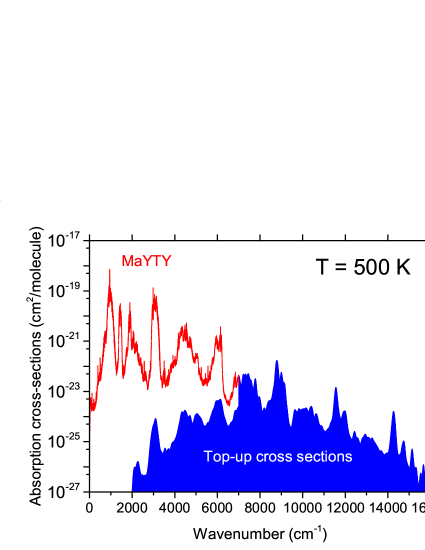
Figure 11: The vibrational ‘top-up’ cross sections of C₂H₄ computed using the vibrational line list with the 3-band model at $T=500$ K (dark blue area) and the ro-vibrational intensities generated using the ExoMol line list with the Gaussian line profile of HWHM=1 cm^-1 (red line).

5 Conclusions

We have produced a new line list for ¹²C₂¹H₄ called MaYTY. Energy levels were calculated variationally using the TROVE program on a refined potential energy surface and transition intensities calculated with a new ab initio dipole moment surface. The MaYTY line list includes transitions between ro-vibrational states with $J\leq 78$ and covers the frequency region up to 7000 cm^-1. Based on analysis of the partition function the variational line list is applicable up to 700 K beyond which opacity will be underestimated. Our line list is in good agreement with experimental intensities from the HITRAN database and experimental cross sections from the PNNL database. The MaYTY line list is available from the CDS (http://cdsarc.u-strasbg.fr) and ExoMol (www.exomol.com) data bases.

To extend the temperature range of applicability of the line list we have implemented a new approximate method of producing absorption cross sections from vibrational ($J=0$) energies and transition moments. The vibrational line list of C₂H₄ is also provided as part of the MaYTY data set. Using this approach we have also generated vibrational cross sections of C₂H₄ covering the wavenumber range up to 12 000 cm^-1 and covering temperatures up to $T=1500$ K. The vibrational cross sections based on the 3-band model can be also generated using a vibrational version of ExoCross. This program, vibrational cross sections and vibrational line list for ethylene are available from the CDS and ExoMol data bases. The $J=0$ method proposed should be useful for calculating opacities of larger molecules where high $J$ variational calculations are extremely challenging.

6 Acknowledgements

This work was supported by the UK Science and Technology Research Council (STFC) No. ST/M001334/1 and the COST action MOLIM No. CM1405. This work made extensive use of UCL’s Legion and DARWIN and COSMOS high performance computing facilities provided by DiRAC for particle physics, astrophysics and cosmology and supported by STFC and BIS.

References

- Adler et al. (2007) Adler T., Knizia G., Werner H.-J., 2007, J. Chem. Phys., 127, 221106
- Al-Refaie et al. (2015a) Al-Refaie A. F., Ovsyannikov R. I., Polyansky O. L., Yurchenko S. N., Tennyson J., 2015a, J. Mol. Spectrosc., 318, 84
- Al-Refaie et al. (2015b) Al-Refaie A. F., Yurchenko S. N., Yachmenev A., Tennyson J., 2015b, Mon. Not. R. Astron. Soc., 448, 1704
- Al-Refaie et al. (2016) Al-Refaie A. F., Polyansky O. L., I. R., Ovsyannikov Tennyson J., Yurchenko S. N., 2016, Mon. Not. R. Astron. Soc., 461, 1012
- Al-Refaie et al. (2017) Al-Refaie A. F., Tennyson J., Yurchenko S. N., 2017, Comput. Phys. Commun., 214, 216
- Atreya et al. (2003) Atreya S. K., Maha P. R., Niemann H. B., Wong M. H., Owen T. C., 2003, Planet Space Sci., 51, 105
- Atreya et al. (2007) Atreya S. K., Mahaffy P. R., Wong A.-S., 2007, Planet Space Sci., 55, 358
- Avila & Carrington (2011) Avila G., Carrington T., 2011, J. Chem. Phys., 135, 064101
- Bach et al. (1998) Bach M., Georges R., Hepp M., Herman M., 1998, Chem. Phys. Lett., 294, 533
- Bach et al. (1999) Bach M., Georges R., Herman M., 1999, Mol. Phys., 97, 265
- Beaulieu et al. (2011) Beaulieu J. P., et al., 2011, Astrophys. J., 731, 16
- Betz (1981) Betz A. L., 1981, Astrophys. J., 244, L103
- Blass et al. (2001) Blass W. E., et al., 2001, J. Quant. Spectrosc. Radiat. Transf., 71, 47
- Bunker & Jensen (1998) Bunker P. R., Jensen P., 1998, Molecular Symmetry and Spectroscopy, 2 edn. NRC Research Press, Ottawa
- Carter et al. (2012) Carter S., Sharma A. R., Bowman J. M., 2012, J. Chem. Phys., 137, 154301
- Consalvi & Liu (2015) Consalvi J. L., Liu F., 2015, Fire Safety J., 78, 202
- Cooley (1961) Cooley J. W., 1961, Math. Comp., 15, 363
- Delahaye et al. (2014) Delahaye T., Nikitin A., Rey M., Szalay P. G., Tyuterev V. G., 2014, J. Chem. Phys., 141, 104301
- Delahaye et al. (2015) Delahaye T., Nikitin A. V., Rey M., Szalay P. G., Tyuterev V. G., 2015, Chem. Phys. Lett., 639, 275
- Fonfria et al. (2017) Fonfria J. P., Hinkle K. H., Cernicharo J., Richter M. J., Agundez M., Wallace L., 2017, Astrophys. J., 835, 196
- Gamache et al. (2017) Gamache R. R., et al., 2017, J. Quant. Spectrosc. Radiat. Transf., 203, 70
- Georges et al. (1999) Georges R., Bach M., Herman M., 1999, Mol. Phys., 97, 279
- Gladston et al. (1996) Gladston R. G., Allen M., Yung Y. L., 1996, Icarus, 119, 1
- Gordon & et al. (2017) Gordon I. E., et al. 2017, J. Quant. Spectrosc. Radiat. Transf., 203, 3
- Guerlet et al. (2009) Guerlet S., Fouchet T., Bézard B., Simon-miller A. A., Flasar F. M., 2009, Icarus, 203, 214
- Hättig (2005) Hättig C., 2005, Phys. Chem. Chem. Phys., 7, 59
- Hill et al. (2009) Hill J. G., Peterson K. A., Knizia G., Werner H.-J., 2009, J. Chem. Phys., 131, 194105
- Hu & Seager (2014) Hu R., Seager S., 2014, Astrophys. J., 784, 63
- Jornet-Somoza et al. (2012) Jornet-Somoza J., Lasorne B., Robb M. A., Dieter Meyer H., Lauvergnat D., Gatti F., 2012, J. Chem. Phys., 137, 084304
- Krylov et al. (1998) Krylov A. I., Sherrill C. D., Byrd E. F. C., Head-gordon M., 1998, J. Chem. Phys., 109, 10669
- Lunine (1993) Lunine J. I., 1993, Annu. Rev. Astron. Astrophys., 31, 217
- Martin et al. (1995) Martin J. M. L., Lee T. J., Taylor P. R., Francois J. P., 1995, J. Chem. Phys., 103, 2589
- Meurer et al. (2017) Meurer A., et al., 2017, PeerJ Comp. Sci., 3, e103
- Niemann et al. (2005) Niemann H. B., et al., 2005, Nature, 438, 779
- Noumerov (1924) Noumerov B. V., 1924, Mon. Not. Roy. Astron. Soc., 84, 592
- Owens et al. (2015) Owens A., Yurchenko S. N., Yachmenev A., Tennyson J., Thiel W., 2015, J. Chem. Phys., 142, 244306
- Owens et al. (2017) Owens A., Yurchenko S. N., Yachmenev A., Thiel W., Tennyson J., 2017, Mon. Not. R. Astron. Soc., 471, 5025
- Partridge & Schwenke (1997) Partridge H., Schwenke D. W., 1997, J. Chem. Phys., 106, 4618
- Peterson et al. (2008) Peterson K. A., Adler T. B., Werner H.-J., 2008, J. Chem. Phys., 128, 084102
- Polyansky et al. (2013) Polyansky O. L., Kozin I. N., Maĺyszek P., Koput J., Tennyson J., Yurchenko S. N., 2013, J. Phys. Chem. A, 117, 7367
- Rey et al. (2016) Rey M., Delahaye T., Nikitin A. V., Tyuterev V. G., 2016, Astron. Astrophys., 594, A47
- Rotger et al. (2008) Rotger M., Boudon V., Auwera J. V., 2008, J. Quant. Spectrosc. Radiat. Transf., 109, 952
- Rusinek et al. (1998) Rusinek E., Fichoux H., Khelkhal M., Herlemont F., Legrand J., Fayt A., 1998, J. Mol. Spectrosc., 189, 64
- Sagan et al. (1993) Sagan C., Thompson W. R., Carlson R., Gurnett D., Hord C., 1993, Nature, 365, 715
- Sharpe et al. (2004) Sharpe S. W., Johnson T. J., Sams R. L., Chu P. M., Rhoderick G. C., Johnson P. A., 2004, Applied Spec., 58, 1452
- Sousa-Silva et al. (2013) Sousa-Silva C., Yurchenko S. N., Tennyson J., 2013, J. Mol. Spectrosc., 288, 28
- Sousa-Silva et al. (2015) Sousa-Silva C., Al-Refaie A. F., Tennyson J., Yurchenko S. N., 2015, Mon. Not. R. Astron. Soc., 446, 2337
- Stofan et al. (2007) Stofan E. R., et al., 2007, Nature, 445, 61
- Swain et al. (2008) Swain M. R., Vasisht G., Tinetti G., 2008, Nature, 452, 329
- Tennyson & Yurchenko (2012) Tennyson J., Yurchenko S. N., 2012, Mon. Not. R. Astron. Soc., 425, 21
- Tennyson & Yurchenko (2017) Tennyson J., Yurchenko S. N., 2017, Intern. J. Quantum Chem., 117, 92
- Tennyson et al. (2016) Tennyson J., et al., 2016, J. Mol. Spectrosc., 327, 73
- Tinetti et al. (2013) Tinetti G., Encrenaz T., Coustenis A., 2013, Astron. Astrophys. Rev., 21, 1
- Underwood et al. (2013) Underwood D. S., Tennyson J., Yurchenko S. N., 2013, Phys. Chem. Chem. Phys., 15, 10118
- Underwood et al. (2016a) Underwood D. S., Tennyson J., Yurchenko S. N., Huang X., Schwenke D. W., Lee T. J., Clausen S., Fateev A., 2016a, Mon. Not. R. Astron. Soc., 459, 3890
- Underwood et al. (2016b) Underwood D. S., Tennyson J., Yurchenko S. N., Clausen S., Fateev A., 2016b, Mon. Not. R. Astron. Soc., 462, 4300
- Waite et al. (2006) Waite J. H., et al., 2006, Science, 311, 1419
- Wang et al. (2015) Wang X., Carter S., Bowman J. M., 2015, J. Phys. Chem. A, 119, 11632
- Weigend (2002) Weigend F., 2002, Phys. Chem. Chem. Phys., 4, 4285
- Werner et al. (2012) Werner H.-J., Knowles P. J., Knizia G., Manby F. R., Schütz M., 2012, WIREs Comput. Mol. Sci., 2, 242
- Western (2017) Western C. M., 2017, J. Quant. Spectrosc. Radiat. Transf., 186, 221
- Yachmenev & Yurchenko (2015) Yachmenev A., Yurchenko S. N., 2015, J. Chem. Phys., 143, 014105
- Yousaf & Peterson (2008) Yousaf K. E., Peterson K. A., 2008, J. Chem. Phys., 129, 184108
- Yurchenko & Tennyson (2014) Yurchenko S. N., Tennyson J., 2014, Mon. Not. R. Astron. Soc., 440, 1649
- Yurchenko et al. (2005) Yurchenko S. N., Thiel W., Carvajal M., Lin H., Jensen P., 2005, Adv. Quant. Chem., 48, 209
- Yurchenko et al. (2007) Yurchenko S. N., Thiel W., Jensen P., 2007, J. Mol. Spectrosc., 245, 126
- Yurchenko et al. (2009) Yurchenko S. N., Barber R. J., Yachmenev A., Thiel W., Jensen P., Tennyson J., 2009, J. Phys. Chem. A, 113, 11845
- Yurchenko et al. (2011a) Yurchenko S. N., Barber R. J., Tennyson J., Thiel W., Jensen P., 2011a, J. Mol. Spectrosc., 268, 123
- Yurchenko et al. (2011b) Yurchenko S. N., Barber R. J., Tennyson J., 2011b, Mon. Not. R. Astron. Soc., 413, 1828
- Yurchenko et al. (2014) Yurchenko S. N., Tennyson J., Bailey J., Hollis M. D. J., Tinetti G., 2014, Proc. Nat. Acad. Sci., 111, 9379
- Yurchenko et al. (2017a) Yurchenko S. N., Yachmenev A., Ovsyannikov R. I., 2017a, J. Chem. Theory Comput., 13, 4368
- Yurchenko et al. (2017b) Yurchenko S. N., Amundsen D. S., Tennyson J., Waldmann I. P., 2017b, Astron. Astrophys., 605, A95