On Embedding of Multidimensional Morse-Smale Diffeomorphisms into Topological Flows

Abstract

J. Palis found necessary conditions for a Morse-Smale diffeomorphism on a closed $n$-dimensional manifold $M^{n}$ to embed into a topological flow and proved that these conditions are also sufficient for $n=2$. For the case $n=3$ a possibility of wild embedding of closures of separatrices of saddles is an additional obstacle for Morse-Smale cascades to embed into topological flows. In this paper we show that there are no such obstructions for Morse-Smale diffeomorphisms without heteroclinic intersection given on the sphere $S^{n},\,n\geq 4$, and Palis’s conditions again are sufficient for such diffeomorphisms.

1 Introduction and statements of results

Let $M^{n}$ be a smooth connected closed $n$-manifold. Recall that a $C^{m}$-flow ($m\geq 0$) on the manifold $M^{n}$ is a continuously depending on $t\in\mathbb{R}$ family of $C^{m}$-diffeomorphisms $X^{t}:M^{n}\to M^{n}$ that satisfies the following conditions:

• $X^{0}(x)=x$ for any point $x\in M^{n}$;

• $X^{t}(X^{s}(x))=X^{t+s}(x)$ for any $s,t\in\mathbb{R}$, $x\in M^{n}$.

A $C^{0}$-flow is also called a topological flow. One says that a homeomorphism (diffeomorphism) $f:M^{n}\to M^{n}$ embeds into a $C^{m}$-flow on $M^{n}$ if $f$ is the time one map of this flow.

Obviously, if a homeomorphism embeds in a flow then it is isotopic to identity. For a homeomorphism of the line and a connected subset of the line this condition also is necessary (see [6],[8]). If an orientation preserving homeomorphism $f$ of the circle satisfies either one of the three conditions: 1) $f$ has a fixed point, 2) $f$ has a dense orbit, or 3) $f$ is periodic then it embeds in a flow (see [7]). Sufficient conditions of embedding in topological flow for a homeomorphisms of a compact two-dimensional disk and of the plane one can find in review [35]. An analytical, $\varepsilon-$closed to the identity diffeomorphism $f:M^{n}\to M^{n}$ can be approximated with accuracy $e^{-\frac{c}{\varepsilon}}$ by a diffeomorphism which embeds in an analytical flow, see [34].

Due to [27] the set of $C^{r}$-diffeomorphisms ($r\geq 1$) which embed in $C^{1}$-flows is a subset of the first category in $Diff^{r}(M^{n})$. As Morse-Smale diffeomorphisms are structurally stable (see [26], [28]) then for any manifold $M^{n}$ there exists an open set (in $Diff^{1}(M^{n})$) of Morse-Smale diffeomorphisms embeddable in topological flows. This set contains neighborhoods of time one maps of Morse-Smale flows without periodic trajectories (according to [30] such flows exist on an arbitrary smooth manifold).

Recall that a diffeomorphism $f:M^{n}\to M^{n}$ is called a Morse-Smale diffeomorphism if it satisfies the following conditions:

• the non-wandering set $\Omega_{f}$ is finite and consists of hyperbolic periodic points;

• for any two points $p,q\in\Omega_{f}$ the intersection of the stable manifold $W^{s}_{p}$ of the point $p$ and the unstable manifold $W^{u}_{q}$ of the point $q$ is transversal.

In [26] J. Palis established the following necessary conditions of the embedding of a Morse-Smale diffeomorphism $f:M^{n}\to M^{n}$ into a topological flow (we call them Palis conditions):

• the non-wandering set $\Omega_{f}$ coincides with the set of fixed points of $f$;

• the restriction of the diffeomorphism $f$ to each invariant manifold of a fixed point $p\in\Omega_{f}$ preserves the orientation of the manifold;

• if for two distinct saddle points $p,q\in\Omega_{f}$ the intersection $W^{s}_{p}\cap W^{u}_{q}$ is not empty then it contains no compact connected components.

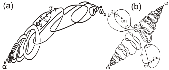
Figure 1: Phase portraits of Morse-Smale diffeomorphisms on $S^{3}$ which do not embed in topological flows

According to [26] these conditions are not only necessary but also sufficient for the case $n=2$. For the case $n=3$ a possibility of wild embedding of closures of separatrices of saddles is another obstruction for Morse-Smale cascades to embed in topological flows (phase portraits of such diffeomorphisms are shown on the Figure 1). In [12] examples of such cascades are described and a criteria for embedding of Morse-Smale 3-diffeomorphisms in topological flows is provided. In the present paper we establish that the Palis conditions are sufficient for Morse-Smale diffeomorphisms on $S^{n},\,n\geq 4,$ such that for any distinct saddle points $p,q\in\Omega_{f}$ the intersection $W^{s}_{p}\cap W^{u}_{q}$ is empty.

Theorem 1.

Suppose that a Morse-Smale diffeomorphism $f:S^{n}\to S^{n}$, $n\geq 4$ satisfies the following conditions:

• the non-wandering set $\Omega_{f}$ of the diffeomorphism $f$ coincides with the set of its fixed points;

• the restriction of $f$ to each invariant manifold of a fixed point $p\in\Omega_{f}$ preserves the orientation of the manifold;

• the invariant manifolds of distinct saddle points of $f$ do not intersect.

  Then $f$ embeds into a topological flow.

Acknowledgments. Research is done with financial support of Russian Science Foundation (project 17-11-01041) apart the section 4.3, which is done in frame of the Basic Research Program of HSE in 2018.

2 Comments to Theorem 1

Due to [26] the conditions $i)$ and $ii)$ are necessary for embedding a Morse-Smale diffeomorphism into a flow. Our condition that the ambient manifold is the sphere $S^{n}$ and the absence of heteroclinic intersections (condition iii)) are not necessary but violation of each of them allows to construct examples of Morse-Smale diffeomorphisms which do not embed in topological flows. Below we describe such examples.

In [23] V. Medvedev and E. Zhuzhoma constructed a Morse-Smale diffeomorphism $f_{0}:M^{4}\to M^{4}$ satisfying conditions $i)-iii)$ on a projective-like manifold $M^{4}$ (different from $S^{4}$) whose non-wandering set consists of exactly three fixed points: a source, a sink and a saddle. Invariant manifolds of the saddle are two-dimensional and the closure of each of them is a wild sphere (see [23], Theorem 4, item 2). Assume that $f_{0}$ embeds in a topological flow $X^{t}_{0}$. Then $X^{t}_{0}$ is a topological flow whose the non-wandering set consists of three equilibrium points with locally hyperbolic behavior. According to [36, Theorem 3] the closures of the invariant manifolds of the saddles are locally flat spheres. That is a contradiction because the closures of the invariant manifolds of the saddle singularities of $X^{t}_{0}$ and $f_{0}$ coincide. Thus, $f_{0}$ does not embed into a flow.

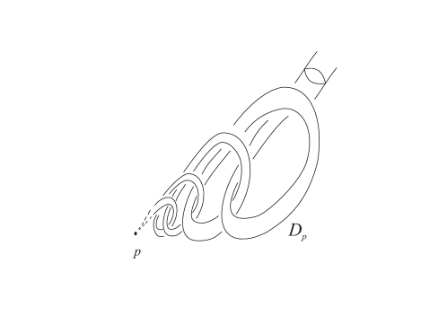
Figure 2: The disk $D_{p}\subset W^{s}_{p}$

In [24] T.Medvedev and O. Pochinka constructed an example of Morse-Smale diffeomorphism $f_{1}:S^{4}\to S^{4}$ satisfying to the conditions $i)-ii)$ of the Theorem 1. The non-wandering set of the diffeomorphism $f_{1}$ consists of two sources, two sinks and two saddles $p,q$ such that $dim\leavevmode\nobreak\ W^{s}_{p}=dim\leavevmode\nobreak\ W^{u}_{q}=3$. The intersection $W^{s}_{p}\cap W^{u}_{q}$ is not empty and its closure in $W^{s}_{p}$ is a wildly embedded open disk $D_{p}$ (see Fig. 2). If $S^{2}\subset W^{s}_{p}$ is a 2-sphere which bounds an open ball containing the point $p$ then the intersection $S^{2}\cap D_{p}$ contains at least three connected components. Assume that $f_{1}$ embeds into a topological flow $X^{t}_{1}$. Then due to [12] the restriction $X^{t}_{p}$ of $X^{t}_{1}$ to $W^{s}_{p}\setminus p$ is topologically conjugated by means of a homeomorphism $h:W^{s}_{p}\setminus p\to\mathbb{S}^{2}\times\mathbb{R}$ to a shift flow $\chi^{t}(s,r)=(s,r+t),\,(s,r)\in\mathbb{S}^{2}\times\mathbb{R}$. Let $\Sigma=h^{-1}(\mathbb{S}^{2}\times\{0\})$. Then every trajectory of the flow $X^{t}_{p}$ intersects the sphere $\Sigma$ at a unique point. Since the disk $D_{p}$ is invariant with respect to the flow $X^{t}_{p}$ the intersection $D_{p}\cap\Sigma$ consists of a unique connected component and that is a contradiction. Thus, $f_{1}$ does not embed into a flow.

3 The scheme of the proof of Theorem 1

The proof of Theorem 1 is based on the technique developed for classification of Morse-Smale diffeomorphisms on orientable manifolds in a series of papers [2], [3], [4], [9], [17], [18], [11],[13]. The idea of the proof consists of the following.

In section 4 we introduce a notion of Morse-Smale homeomorphism on a topological n-manifold and define the subclass $G(S^{n})$ of such homeomorphisms satisfying to conditions similar to $i)-iii)$ of Theorem 1.

Let $f\in G(S^{n})$. In [13, Theorem 1.3] it is shown that the dimension of the invariant manifolds of the fixed points of $f$ can be only one of $0,1,n-1$ or $n$. Denote by $\Omega^{i}_{f}$ the set of all fixed points of $f$ whose unstable manifolds have dimension $i\in\{0,1,n-1,n\}$, and by $m_{f}$ the number of all saddle points of $f$.

Represent the sphere $S^{n}$ as the union of pairwise disjoint sets

$$A_{f}=(\bigcup\limits_{\sigma\in\Omega^{1}_{f}}{W^{u}_{\sigma}})\cup\Omega^{0}_{f},\,R_{f}=(\bigcup\limits_{\sigma\in\Omega^{n-1}_{f}}{W^{s}_{\sigma}})\cup\Omega^{n}_{f},\,V_{f}=S^{n}\setminus(A_{f}\cup R_{f}).$$

Similar to [16] one can prove that the sets $A_{f},R_{f},V_{f}$ are connected, the set $A_{f}$ is an attractor, $R_{f}$ is a repeller and $V_{f}$ consists of wandering orbits of $f$ moving from $R_{f}$ to $A_{f}$.

Denote by $\widehat{V}_{f}=V_{f}/f$ the orbit space of the action of $f$ on $V_{f}$ and by $p_{{}_{f}}:V_{f}\to\widehat{V}_{f}$ the natural projection. Let

$$\hat{L}^{s}_{f}=\bigcup\limits_{\sigma\in\Omega^{1}_{f}}p_{{}_{f}}(W^{s}_{\sigma}\setminus\sigma),\,\,\,\hat{L}^{u}_{f}=\bigcup\limits_{\sigma\in\Omega^{n-1}_{f}}p_{{}_{f}}(W^{u}_{\sigma}\setminus\sigma).$$

Definition 3.1.

The collection $S_{f}=(\widehat{V}_{f},\hat{L}^{s}_{f},\hat{L}^{u}_{f})$ is called the scheme of the homeomorphism $f\in G(S^{n})$.

Definition 3.2.

Schemes $S_{f}$ and $S_{f^{\prime}}$ of homeomorphisms $f,f^{\prime}\in G(S^{n})$ are called equivalent if there exists a homeomorphism $\hat{\varphi}:\widehat{V}_{f}\to\widehat{V}_{f^{\prime}}$ such that $\hat{\varphi}(\hat{L}^{s}_{f})=\hat{L}^{s}_{f^{\prime}}$ and $\hat{\varphi}(\hat{L}^{u}_{f})=\hat{L}^{u}_{f^{\prime}}$.

The next statement follows from paper [13, Theorem 1.2] (in fact, Theorem 1.2 was proven for Morse-Smale diffeomorphisms but the smoothness plays no role in the proof).

Statement 3.1.

Homeomorphisms $f,f^{\prime}\in G(S^{n})$ are topologically equivalent if and only if their schemes $S_{f}$, $S_{f^{\prime}}$ are equivalent.

The possibility of embedding of $f\in G(S^{n})$ into a topological flow follows from triviality of the scheme in the following sense.

Let $a^{t}$ be the flow on the set $\mathbb{S}^{n-1}\times\mathbb{R}$ defined by $a^{t}(x,s)=(x,s+t)$, $x\in S^{n-1},s\in\mathbb{R}$ and let $a$ be the time-one map of $a^{t}$. Let $\mathbb{Q}^{n}=\mathbb{S}^{n-1}\times\mathbb{S}^{1}$. Then the orbit space of the action $a$ on $\mathbb{S}^{n-1}\times\mathbb{R}$ is $\mathbb{Q}^{n}$. Denote by $p_{{}_{\mathbb{Q}^{n}}}:\mathbb{S}^{n-1}\times\mathbb{R}\to\mathbb{Q}^{n}$ the natural projection. Let $m\in\mathbb{N}$ and $c_{1},...,c_{m}\subset\mathbb{S}^{n-1}$ be a collection of smooth pairwise disjoint $(n-2)$-spheres. Let ${Q}^{n-1}_{i}=\bigcup\limits_{t\in\mathbb{R}}a^{t}(c_{i})$, $\mathbb{L}_{m}=\bigcup\limits_{i=1}^{m}Q^{n-1}_{i}$ and $\widehat{\mathbb{L}}_{m}=p_{{}_{\mathbb{Q}^{n}}}(\mathbb{L}_{m})$.

Definition 3.3.

The scheme $S_{f}=(\widehat{V}_{f},\hat{L}^{s}_{f},\hat{L}^{u}_{f})$ of a homeomorphism $f\in G(S^{n})$ is called trivial if there exists a homeomorphism $\hat{\psi}:\widehat{V}_{f}\to\mathbb{Q}^{n}$ such that $\hat{\psi}(\hat{L}^{s}_{f}\cup\hat{L}^{u}_{f})=\widehat{\mathbb{L}}_{m_{f}}$.

In the section 5 we prove the following key lemma.

Lemma 3.1.

If $f\in G(S^{n})$ then its scheme $S_{f}$ is trivial.

In the section 6 we construct a topological flow $X^{t}_{f}$ whose time one map belongs to the class $G(S^{n})$ and has the scheme equivalent to $S_{f}$. According to Statement 3.1 there exists a homeomorphism $h:S^{n}\to S^{n}$ such that $f=hX^{1}_{f}h^{-1}$. Then the homeomorphism $f$ embeds into the topological flow $Y^{t}_{f}=hX^{t}_{f}h^{-1}$.

4 Morse-Smale homeomorphisms

This section contains some definitions and statements which was introduced and proved in [14].

4.1 Basic definitions

Remind that a linear automorphism $L:\mathbb{R}^{n}\to\mathbb{R}^{n}$ is called hyperbolic if its matrix has no eigenvalues with absolute value equal one. In this case a space $\mathbb{R}^{n}$ have a unique decomposition into the direct sum of $L$-invariant subsets $E^{s},E^{u}$ such that $||L|_{E^{s}}||<1$ and $||L^{-1}|_{E^{u}}||<1$ in some norm $||\cdot||$ (see, for example, Propositions 2.9, 2.10 of Chapter 2 in [25]).

According to Proposition 5.4 of the book [25] any hyperbolic automorphism $L$ is topologically conjugated with a linear map of the following form:

$$a_{\lambda,\mu,\nu}(x_{1},x_{2},...,x_{\lambda},x_{\lambda+1},x_{\lambda+2},...,x_{n})=(2\mu x_{1},2x_{2},...,2x_{\lambda},\frac{1}{2}\nu x_{\lambda+1},\frac{1}{2}x_{\lambda+2},...,\frac{1}{2}x_{n}),$$ (1)

where $\lambda=dim\,E^{u}\in\{0,1,...,n\}$, $\mu=-1$ ($\mu=1$) if the restriction $L|_{E^{u}}$ reverses (preserves) an orientation of $E^{u}$, and $\nu=-1$ ($\nu=1$) if the restriction $L|_{E^{s}}$ reverses (preserves) an orientation of $E^{s}$.

Put ${\mathbb{E}^{s}_{\lambda}}=\{(x_{1},...,x_{n})\in\mathbb{R}^{n}|\ x_{1}=x_{2}=\dots=x_{\lambda}=0\}$, ${\mathbb{E}^{u}_{\lambda}}=\{(x_{1},...,x_{n})\in\mathbb{R}^{n}|\ x_{\lambda+1}=x_{\lambda+2}=\dots=x_{n}=0\}$ and denote by $P^{s}_{x}(P^{u}_{y})$ a hyperplane that parallel to the hyperplane $\mathbb{E}^{s}_{\lambda}$ ($\mathbb{E}^{u}_{\lambda}$) and contain a point $x\in\mathbb{E}^{u}_{\lambda}$ ($y\in\mathbb{E}^{s}_{\lambda}$). Unions $\mathcal{P}^{s}_{\lambda}=\{P^{s}_{x}\}_{x\in\mathbb{E}^{u}_{\lambda}},\mathcal{P}^{u}_{\lambda}=\{P^{u}_{y}\}_{y\in\mathbb{E}^{s}_{\lambda}}$ form the $a_{\lambda,\mu,\nu}$-invariant foliation.

Suppose that $M^{n}$ is an $n$-dimensional topological manifold, $f:M^{n}\to M^{n}$ is a homeomorphism and $p$ is a fixed point of the homeomorphism $f$. We will call the point $p$ topologically hyperbolic point of index $\lambda_{p}$, if there exists its neighborhood $U_{p}\subset M^{n}$, numbers $\lambda_{p}\in\{0,1,...,n\},\mu_{p},\nu_{p}\in\{+1,-1\}$, and a homeomorphism $h_{p}:U_{p}\to\mathbb{R}^{n}$ such that $h_{p}f|_{U_{p}}=a_{\lambda_{p},\mu_{p},\nu_{p}}h_{p}|_{U_{p}}$ when the left and right parts are defined. Call the sets $W^{s}_{p,loc}=h_{p}^{-1}(E^{s}),{W}^{u}_{p,loc}=h_{p}^{-1}(E^{u})$ the local invariant manifolds of the point $p$, and the sets $W^{s}_{p}=\bigcup\limits_{i\in\mathbb{Z}}f^{i}({W}^{s}_{p,loc})$, $W^{u}_{p}=\bigcup\limits_{i\in\mathbb{Z}}f^{i}({W}^{u}_{p,loc})$ the stable and unstable invariant manifolds of the point $p$.

It follows form the definition that $W^{s}_{p}=\{x\in M^{n}:\lim\limits_{i\to+\infty}f^{i}(x)=p\},W^{u}_{p}=\{x\in M^{n}:\lim\limits_{i\to+\infty}f^{-i}(x)=p\}$ and $W^{u}_{p}\cap W^{u}_{q}=\emptyset$ ($W^{s}_{p}\cap W^{s}_{q}=\emptyset$) for any distinct hyperbolic points $p,q$. Moreover, there exists an injective continuous immersion $J:\mathbb{R}^{\lambda_{p}}\to M^{n}$ such that $W^{u}_{p}=J(\mathbb{R}^{{\lambda_{p}}})$.

A hyperbolic fixed point is called the source (the sinks) if its indice equals $n$ ($0$), a hyperbolic fixed point $p$ of index $0<\lambda_{p}<n$ is called the saddle point.

A periodic point $p$ of period $m_{p}$ of a homeomorphism $f$ is called a topologically hyperbolic sink $($ source, saddle$)$ periodic point if it is the topologically hyperbolic $($source, saddle$)$ fixed point for the homeomorphism $f^{m_{p}}$. The stable and unstable manifolds of the periodic point $p$ considered as the fixed point of the homeomorphism $f^{m_{p}}$ are called the stable and unstable manifolds of the point $p$. Every connected component of the set $W^{s}_{p}\setminus p$ ($W^{u}_{p}\setminus p$) is called the stable $($ the unstable$)$ separatrix and is denoted by $l^{s}_{p}$ ($l^{u}_{p}$).

The linearizing homeomorphism $h_{p}:U_{p}\to\mathbb{R}^{n}$ induces a pair of transversal foliations $\mathcal{F}^{s}_{p}=h_{p}^{-1}(\mathcal{P}^{s}_{\lambda_{p}})$ , $\mathcal{F}^{u}_{p}=h_{p}^{-1}(\mathcal{P}^{u}_{\lambda_{p}})$ on the set $U_{p}$. Every leaf of the foliation $\mathcal{F}^{s}_{p}\ (\mathcal{F}^{u}_{p})$ is an open disk of dimension $\lambda_{p}\ (n-\lambda_{p})$. For any point $x\in U_{p}$ denote by $F^{s}_{p,x},F^{u}_{p,x}$ the leaf of the foliation $\mathcal{F}^{s}_{p},\mathcal{F}^{u}_{p}$, correspondingly, containing the point $x$.

The invariant manifolds $W^{s}_{p}$ and $W^{u}_{q}$ of saddle periodic points $p,q$ of a homeomorphism $f$ intersect consistently transversally if one of the following conditions holds:

1. $W^{s}_{p}\cap W^{u}_{q}=\emptyset$;

2. $W^{s}_{p}\cap W^{u}_{q}\neq\emptyset$ and $F^{s}_{q,x}\subset W^{s}_{p}$; $F^{u}_{p,y}\subset W^{u}_{q}$ for any points $x\in W^{s}_{p}\cap U_{q}$, $y\in W^{u}_{q}\cap U_{p}$.

Definition 4.1.

A homeomorphism $f:M^{n}\to M^{n}$ is called the Morse-Smale homeomorphism if it satisfies the next conditions:

1. its non-wandering set $\Omega_{f}$ finite and any point $p\in\Omega_{f}$ is topologically hyperbolic;

2. invariant manifolds of any two saddle points $p,q\in\Omega_{f}$ intersect consistently transversally.

4.2 Properties of Morse-Smale homeomorphisms

Statement 4.1.

Let $f:M^{n}\to M^{n}$ be a Morse-Smale homeomorphism. Then:

1. $W^{u}_{p}\cap W^{s}_{p}=p$ for any saddle point $p\in\Omega_{f}$;

2. for any saddle points $p,q,r\in\Omega_{f}$ the conditions $(W^{s}_{p}\setminus p)\cap(W^{u}_{q}\setminus q)\neq\emptyset$, $(W^{s}_{q}\setminus q)\cap(W^{u}_{r}\setminus r)\neq\emptyset$ imply $(W^{s}_{p}\setminus p)\cap(W^{u}_{r}\setminus r)\neq\emptyset$;

3. there are no sequence of distinct saddle points $p_{1},p_{2},...,p_{k}\in\Omega_{f}$, $k>1$, such that $(W^{s}_{p_{i}}\setminus p_{i})\cap(W^{u}_{p_{i+1}}\setminus p_{i+1})\neq\emptyset$ for $i\in\{1,...,k-1\}$ and $(W^{s}_{p_{k}}\setminus p_{k})\cap(W^{u}_{p_{1}}\setminus p_{1})\neq\emptyset$.

Statement 4.2.

Let $f:M^{n}\to M^{n}$ be a Morse-Smale homeomorphism. Then:

1. $M^{n}=\bigcup\limits_{p\in\Omega_{f}}W^{u}_{p}$;

2. for any point $p\in\Omega_{f}$ the manifold $W^{u}_{p}$ is a topological submanifold of the manifold $M^{n}$;

3. for any point $p\in\Omega_{f}$ and any connected component $l^{u}_{p}$ of the set $W^{u}_{p}\setminus p$ the following equality holds: $cl\,{l^{u}_{p}}\setminus(l^{u}_{p}\cup p)=\bigcup\limits_{q\in\Omega_{f}:W^{s}_{q}\cap l^{u}_{p}\neq\emptyset}W^{u}_{q}$ .

Corollary 4.1.

If $f:M^{n}\to M^{n}$ is a Morse-Smale homeomorphism and $p\in\Omega_{f}$ is a saddle point such that $l^{u}_{p}\cap W^{s}_{q}=\emptyset$ for any saddle point $q\neq p$, then there exists a unique sink $\omega\in\Omega_{f}$ such that $cl\,l^{u}_{p}=l^{u}_{p}\cup p\cup\omega$ and $cl\,l^{u}_{p}$ is either a compact arc in case $\lambda_{p}=1$ or a sphere of dimension $\lambda_{p}$ in case $\lambda_{p}>1$.

For an arbitrary point $q\in\Omega_{f}$ and $\delta\in\{u,s\}$ put $V^{\delta}_{q}=W^{\delta}_{q}\setminus q$ and denote by $\widehat{V}^{\delta}_{q}=V^{s}_{q}/f$ the orbit space of the action of the homeomorphism $f$ on the set $V^{\delta}_{q}$. The following statement is proved in the book [9] (Proposition 2.1.5).

Statement 4.3.

The space $\widehat{V}^{u}_{q}$ is homeomorphic to $\mathbb{S}^{\lambda_{q}-1}\times\mathbb{S}^{1}$ and the space $\widehat{V}^{s}_{q}$ is homeomorphic to $\mathbb{S}^{n-\lambda_{q}-1}\times\mathbb{S}^{1}$.

Remark that $\mathbb{S}^{0}\times\mathbb{S}^{1}$ means a union of two disjoint closed curves.

Proposition 4.1.

Suppose $f:M^{n}\to M^{n}$ is a Morse-Smale homeomorphism, $n\geq 4$, and $\sigma\in\Omega_{f}$ is a saddle point of index $(n-1)$ such that $l^{u}_{\sigma}\cap W^{s}_{q}=\emptyset$ for any saddle point $q\neq p$. Then the sphere $cl\,{l^{u}_{\sigma}}$ is bicollared.

Proof: Let $\omega\in\Omega^{0}_{f}$ be a sink point such that $l^{u}_{\sigma}\subset W^{s}_{\omega}$. Due to Corollary 4.1 and the item 2 of Statement 4.2 the set $cl\,{l^{u}_{\sigma}}=l^{u}_{\sigma}\cup\omega$ is an $(n-1)$-sphere which is locally flat embedded in $M^{n}$ at all its points apart possibly one point $\omega$. According to [5], [20] an $(n-1)$-sphere in a manifold $M^{n}$ of dimension $n\geq 4$ is either locally flat or have more than countable set of points of wildness. Therefore the sphere $cl\,{l^{u}_{\sigma}}$ is locally flat at point $\omega$. According to [1] a locally flat sphere is bicollared. $\diamond$

By $G(S^{n})$ we denoted a class of Morse-Smale homeomorphism on the sphere $S^{n}$ such that any $f\in G(S^{n})$ satisfy the following conditions:

1. $\Omega_{f}$ consists of fixed points;

2. $W^{s}_{p}\cap W^{u}_{q}=\emptyset$ for any distinct saddle points $p,q\in\Omega_{f}$;

3. the restriction of a homeomorphism $f$ on every invariant manifolds of an arbitrary fixed point $p\in\Omega_{f}$ preserves its orientation.

Proposition 4.2.

If $f\in G(S^{n})$, then any saddle fixed point has index $1$ and $(n-1)$.

Proof: Suppose that, on the contrary, there exists a point $\sigma\in\Omega_{f}$ of index $j\in(1,n-1)$. According to Corollary 4.1 the closures $cl\,{W^{u}_{\sigma}},cl\,{W^{s}_{\sigma}}$ of the stable and unstable manifolds of the point $\sigma$ are spheres of dimensions $j$ and $n-j$ correspondingly. Due to item 1 of Statements 4.1, the spheres $S^{j}=cl\,{W^{u}_{\sigma}},S^{n-j}=cl\,{W^{s}_{\sigma}}$ intersect at a single point $\sigma$. Therefore their intersection index equals either $1$ or $-1$ (depending on the choice of orientations of the spheres $S^{j}$, $S^{n-j}$ and $S^{n}$). Since homology groups $H_{j}(S^{n}),H_{n-j}(S^{n})$ are trivial it follows that there is a sphere $\tilde{S}^{j}$ homological to the sphere $S^{j}$ and having the empty intersection with the sphere $S^{n-j}$. Then the intersection number of the spheres $S^{j},S^{n-j}$ must be equal to zero as the intersection number is the homology invariant (see, for example, [32], $\S\,69$). This contradiction proves the statement. $\diamond$

4.3 Canonical manifolds connected with saddle fixed points of a homeomorphism $f\in G(S^{n})$

It follows from Statement 4.2 that for each saddle point of a homeomorphism $f\in G(S^{n})$ there exists a neighborhood where $f$ is topologically conjugated either with the map $a_{1}:\mathbb{R}^{n}\to\mathbb{R}^{n}$ defined by $a_{1}(x_{1},x_{2},\dots,x_{n})=(2x_{1},\frac{1}{2}x_{2},\dots,\frac{1}{2}x_{n})$ or with the map $a_{1}^{-1}$. In this section we describe canonical manifolds defined by the action of the map $a_{1}$ and prove Proposition 4.3 allowing to define similar canonical manifolds for the homeomorphism $f\in G(S^{n})$.

Put $\mathbb{U}_{\tau}=\{(x_{1},...,x_{n})\in\mathbb{R}^{n}|\ x_{1}^{2}(x_{2}^{2}+...+x_{n}^{2})\leq\tau^{2}\}$, $\tau\in(0,1]$, $\mathbb{U}=\mathbb{U}_{1}$; $\mathbb{U}_{0}=\{(x_{1},...,x_{n})\in\mathbb{R}^{n}|\ x_{1}=0\}$, $\mathbb{N}^{s}=\mathbb{U}\setminus Ox_{1}$, $\mathbb{N}^{u}=\mathbb{U}\setminus\mathbb{U}_{0}$, $\widehat{\mathbb{N}}^{s}=\mathbb{N}^{s}/a_{1}$, $\widehat{\mathbb{N}}^{u}=\mathbb{N}^{u}/a_{1}$. Denote by $p_{s}:\mathbb{N}^{s}\to\widehat{\mathbb{N}}^{s}$, $p_{u}:\mathbb{N}^{u}\to\widehat{\mathbb{N}}^{u}$ the natural projections and put $\widehat{V}^{s}=p_{s}(\mathbb{U}_{0})$.

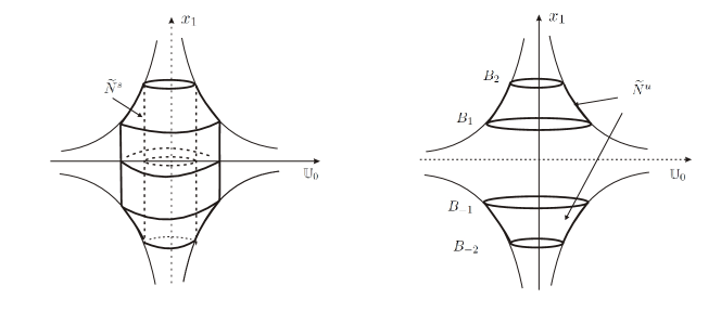
Figure 3: Fundamental domains $\widetilde{N}^{s},\widetilde{N}^{u}$ of the action of the homeomorphism $a_{1}$ on the sets $\mathbb{N}^{s},\mathbb{N}^{u}$

The following statement is proved in [11] (Propositions 2.2, 2.3).

Statement 4.4.

The space $\widehat{\mathbb{N}}^{s}$ is homeomorphic to the direct product $\mathbb{S}^{n-2}\times\mathbb{S}^{1}\times[-1,1]$, the space $\widehat{\mathbb{N}}^{u}$ consists of two connected components each of which is homeomorphic to the direct product $\mathbb{B}^{n-1}\times\mathbb{S}^{1}$.

Recall that an annulus of dimension $n$ is a manifold homeomorphic to $\mathbb{S}^{n-1}\times[0,1]$.

On the Figure 3 we present the neighborhoods $\mathbb{N}^{s},\mathbb{N}^{u}$ and the fundamental domains $\widetilde{N}^{s}=\{(x_{1},\dots,x_{n})\in\mathbb{N}^{s}|\frac{1}{4}\leq x_{2}^{2}+\dots+x_{n}^{2}\leq 1\},\widetilde{N}^{u}=\{(x_{1},\dots,x_{n})\in\mathbb{N}^{u}||x_{1}|\in[1,2]\}$ of the action of the diffeomorphism $a_{1}$. Put $\mathcal{C}=\{\{(x_{1},\dots,x_{n})\in\mathbb{R}^{n}|\frac{1}{4}\leq x_{2}^{2}+\dots+x_{n}^{2}\leq 1\}$. The set $\mathbb{N}^{s}$ is the union of the hyperplanes $\mathcal{L}_{t}=\{(x_{1},...,x_{n})\in{N}^{s}|x_{1}^{2}(x_{2}^{2}+\dots+x_{n}^{2})=t^{2}\},t\in[-1,1]$. Then the fundamental domain $\widetilde{{N}}^{s}$ is the union of the pairs of annuli $\mathcal{K}_{t}=\mathcal{L}_{t}\cap\mathcal{C},t\in[-1,1]$ and the space $\widehat{\mathbb{N}}^{s}$ can be obtained from $\widetilde{{N}}^{s}$ by gluing the connected components of the boundary of each annulus by means of the diffeomorphism $a_{1}$. The set $\widetilde{N}^{u}$ consist of two connected components each of which is homeomorphic to the direct product $\mathbb{B}^{n-1}\times[0,1]$. The space $\widehat{\mathbb{N}}^{u}$ is obtained from $\widetilde{N}^{u}$ by gluing the disk $B_{1}=\{(x_{1},\dots,x_{n})\in\mathbb{N}^{u}|x_{1}=1\}$ to the disk $B_{2}=\{(x_{1},\dots,x_{n})\in\mathbb{N}^{u}|x_{1}=2\}$ and the disk $B_{-1}=\{(x_{1},\dots,x_{n})\in\mathbb{N}^{u}|x_{1}=-1\}$ to the disk $B_{-2}=\{(x_{1},\dots,x_{n})\in\mathbb{N}^{u}|x_{1}=-2\}$ by means of the diffeomorphism $a_{1}$.

Proposition 4.3.

Suppose $f\in G(S^{n})$; then there exists a set of pair-vise disjoint neighborhoods $\{N_{\sigma}\}_{\sigma\in\Omega^{1}_{f}\cup\Omega^{n-1}_{f}}$ such that for any neighborhood $N_{\sigma}$ there exists a homeomorphism $\chi_{\sigma}:N_{\sigma}\to\mathbb{U}$ such that $\chi_{\sigma}f|_{{}_{N_{\sigma}}}=a_{1}\chi_{\sigma}|_{{}_{N_{\sigma}}}$ whenever $\lambda_{\sigma}=1$ and $\chi_{\sigma}f|_{{}_{N_{\sigma}}}=a^{-1}_{1}\chi_{\sigma}|_{{}_{N_{\sigma}}}$ whenever $\lambda_{\sigma}=n-1$.

Proof: Put ${V}^{\delta}_{\Omega^{i}_{f}}=\bigcup\limits_{q\in\Omega^{i}_{f}}{V}^{\delta}_{q}$, $\widehat{V}^{\delta}_{\Omega^{i}_{f}}=\bigcup\limits_{q\in\Omega^{i}_{f}}\widehat{V}^{\delta}_{q}$, $i\in\{0,1,n-1,n\}$, $\delta\in\{s,u\}$ and denote by $p^{\delta}_{\Omega^{i}_{f}}:{V}^{\delta}_{\Omega^{i}_{f}}\to\widehat{V}^{\delta}_{\Omega^{i}_{f}}$ the natural projection such that $p^{\delta}_{\Omega^{i}_{f}}|_{V^{\delta}_{q}}=p^{\delta}_{q}|_{V^{\delta}_{q}}$ for any point $q\in\Omega_{f}$.

Put $\Sigma_{f}=\Omega^{1}_{f}\cup\Omega^{n-1}_{f}$, $\widehat{L}^{u}_{\Sigma_{f}}=p^{s}_{\Omega^{0}_{f}}(V^{u}_{\Omega^{1}_{f}}\cup V^{u}_{\Omega^{n-1}_{f}})$.

The set $\widehat{L}^{u}_{\Sigma_{f}}$ consists of finite number of compact topological submanifolds. Then there is a set of pair-vise disjoint compact neighborhoods $\{\widehat{K}^{u}_{\sigma},\sigma\in\Sigma_{f}\}$ of these manifolds in $\widehat{V}^{s}_{\Omega^{0}}$. For every point $\sigma\in\Sigma_{f}$ put $K^{u}_{\sigma}=(p^{s}_{\Omega^{0}_{f}})^{-1}({\widehat{K}^{u}_{\sigma}})$ and $\widetilde{N}_{\sigma}=K^{u}_{\sigma}\cup W^{s}_{\sigma}$.

Let $U_{\sigma}\subset\widetilde{N}_{\sigma}$ be a neighborhood of the point $\sigma$ such that a homeomorphism $g_{\sigma}:U_{\sigma}\to\mathbb{R}^{n}$ satisfying the condition $g_{\sigma}f|_{U_{\sigma}}=a_{\lambda_{\sigma}}g_{\sigma}|_{U_{\sigma}}$ is defined.

Put $u_{\tau}=\{(x_{1},...,x_{n})\in\mathbb{U}_{\tau}|\ x_{2}^{2}+...+x_{n}^{2}\leq 1,|x_{1}|\leq 2\tau\}$, $D^{u}_{\tau}=\{(x_{1},...,x_{n})\in\mathbb{U}_{\tau}|\ \tau<|x_{1}|\leq 2\tau\}$, $D^{s}_{\tau}=\{(x_{1},...,x_{n})\in\mathbb{U}_{\tau}|\ \frac{1}{4}\leq x_{2}^{2}+...+x_{n}^{2}\leq 1\}$, $\tilde{u}_{\tau}=g_{\sigma}^{-1}(u_{\tau})$, $\widetilde{D}^{\delta}_{\tau}=g_{\sigma}^{-1}(D^{\delta}_{\tau})$, $\delta\in\{s,u\}$, and $N_{\tau}=\bigcup\limits_{i\in\mathbb{Z}}f^{i}(\widetilde{u}_{\tau})$.

Let us show that there is a number $\tau_{1}>0$ such that for any $i\in\mathbb{N}$ the intersection $f^{i}(\widetilde{D}^{u}_{\tau_{1}})\cap\tilde{u}_{\tau_{1}}$ is empty. Suppose $\sigma\in\Omega^{n-1}_{f}$ (the argument for the case $\sigma\in\Omega^{1}_{f}$ is similar). By the Statement 4.2, the set $\bigcup\limits_{i\in\mathbb{N}}f^{i}(\widetilde{D}^{u}_{\tau})$ lies in the stable manifold of a unique sink point $\omega$. Since the homeomorphism $f$ is locally conjugated with the linear compression $a_{0}$ in a neighborhood of the point $\omega$, we have that there exists a ball $B^{n}\subset W^{s}_{\omega}\setminus U_{\sigma}$ such that $\omega\subset B^{n}$ and $f(B^{n})\subset int\leavevmode\nobreak\ B^{n}$. Since $\widetilde{D}^{u}_{\tau}$ is compact, there is $i^{*}>0$ such that $f^{i}(\widetilde{D}^{u}_{\tau})\cap U_{\sigma}\subset B^{n}$ for all $i>i^{*}$. Hence the set of numbers $i_{j}$ such that $f^{i_{j}}(\widetilde{D}^{u}_{\tau})\cap\tilde{u}_{\tau}\neq\emptyset$ is finite. Then one can choose $\tau_{1}\in(0,\tau)$ such that $\tilde{u}_{\tau_{1}}\cap f^{i}(\widetilde{D}^{u}_{\tau}))=\emptyset$ and therefore $\tilde{u}_{\tau_{1}}\cap f^{i}(\widetilde{D}^{u}_{\tau_{1}}))=\emptyset$ for any $i\in\mathbb{N}$. Similarly one can show that there exists a number $\tau_{2}\in(0,\tau_{1}]$ such that for any $i\in\mathbb{N}$ the intersection of $f^{-i}(\widetilde{D}^{s}_{\tau_{2}})\cap\tilde{u}_{\tau_{2}}$ is empty.

Suppose $\lambda_{\sigma}=1$, put $N_{\sigma}=\bigcup\limits_{i\in\mathbb{Z}}f^{i}(\tilde{u}_{\tau_{2}})$, and define a homeomorphism ${\chi^{*}}_{\sigma}:N_{\sigma}\to U_{\tau_{2}}$ by the following: $\chi^{*}_{\sigma}(x)=g_{\sigma}(x)$ whenever $x\in\tilde{u}_{\tau_{2}}$, and $\chi^{*}_{\sigma}(x)=a_{\lambda_{\sigma}}^{-k}(g_{\sigma}(f^{k}(x)))$ whenever $x\in{N}_{\sigma}\setminus(\tilde{u}_{\tau_{2}})$, where $k\in\mathbb{Z}$ is such that $f^{k}(x)\in\tilde{u}_{\tau_{2}}$. The homeomorphism ${\chi^{*}}_{\sigma}$ conjugates the homeomorphism $f|_{N_{\sigma}}$ with the linear diffeomorphism $a_{1}|_{\mathbb{U}_{\tau_{2}}}$. Since the homeomorphism $a_{1}|_{\mathbb{U}_{\tau_{2}}}$ is topologically conjugated with $a_{1}|_{\mathbb{U}}$ by means of the diffeomorphism $g(x_{1},...,x_{n})=\left(\frac{x_{1}}{\sqrt{\tau_{2}}},...,\frac{x_{n}}{\sqrt{\tau_{2}}}\right)$, we see that the superposition $\chi_{\sigma}=g\chi^{*}_{\sigma}:{N}_{\sigma}\to\mathbb{U}$ topologically conjugates $f|_{{N}_{\sigma}}$ with $a_{1}|_{\mathbb{U}}$. A homeomorphism $\chi_{\sigma}$ for the case $\lambda_{\sigma}=n-1$ can be constructed in the same way.

$\diamond$

Put $N^{u}_{\sigma}=N_{\sigma}\setminus W^{s}_{\sigma}$, $N_{\tau,\sigma}=\chi_{\sigma}^{-1}(\mathbb{U}_{\tau})$, $N^{s}_{\sigma}=N_{\sigma}\setminus W^{u}_{\sigma}$, $\widehat{N}^{s}_{\sigma}=N^{s}_{\sigma}/f$, $\widehat{N}^{u}_{\sigma}=N^{u}/f$.

5 Triviality of the scheme of the homeomorphism $f\in G(S^{n})$

This section is devoted to the proof of Lemma 3.1. In subsections 5.1-5.3 we establish some axillary results.

5.1 Introduction results on the embedding of closed curves and their tubular neighborhoods in a manifold $M^{n}$

Further we denote by $M^{n}$ a topological manifold possibly with non-empty boundary.

Recall that a manifold $N^{k}\subset M^{n}$ of dimension $k$ without boundary is locally flat in a point $x\in N^{k}$ if there exists a neighborhood $U(x)\subset M^{n}$ of the point $x$ and a homeomorphism $\varphi:U(x)\to\mathbb{R}^{n}$ such that $\varphi(N^{k}\cap U(x))=\mathbb{R}^{k}$, where $\mathbb{R}^{k}=\{(x_{1},...,x_{n})\in\mathbb{R}^{n}|\ x_{k+1}=x_{k+2}=...=x_{n}=0\}$.

A manifold $N^{k}$ is locally flat in $M^{n}$ or the submanifold of the manifold $M^{n}$ if it is locally flat at each its point.

If the condition of local flatness fails in a point $x\in N^{k}$ then the manifold $N^{k}$ is called wild and the point $x$ is called the point of wildness.

A topological space $X$ is called $m$-connected (for $m>0$) if it is non-empty, path-connected and its first $m$ homotopy groups $\pi_{i}(X)$, $i\in\{1,\dots,m\}$ are trivial. The requirements of being non-empty and path-connected can be interpreted as (-1)-connected and 0-connected correspondingly.

A topological space $P$ generated by points of a simplicial complex $K$ with the topology induced from $\mathbb{R}^{n}$ is called the polyhedron. The complex $K$ is called the partition or the triangulation of the polyhedron $P$.

A map $h:P\to Q$ of polyhedra is called piece-vise linear if there exists partitions $K,L$ of polyhedra $P,Q$ correspondingly such that $h$ move each simplex of the complex $K$ into a simplex of the complex $L$ (see for example [29]).

A polyhedron $P$ is called the piece-vise linear manifold of dimension $n$ with boundary if it is a topological manifold with boundary and for any point $x\in int\,P$ ($y\in\partial P$) there is a neighborhood $U_{x}$ ($U_{y}$) and a piece-vise linear homeomorphism $h_{x}:U_{x}\to\mathbb{R}^{n}$ ($h_{y}:U_{y}\to\mathbb{R}^{n}_{+}=\{(x_{1},...,x_{n})\subset\mathbb{R}^{n}|\ x_{1}\geq 0\}$).

The following important statement follows from Theorem 4 of [19].

Statement 5.1.

Suppose that $N^{k},M^{n}$ are compact piece-vise linear manifolds of dimension $k,n$ correspondingly, $N^{k}$ is the manifold without boundary, $M^{n}$ possibly has a non-empty boundary, $\tilde{e},e:N^{k}\to int\leavevmode\nobreak\ M^{n}$ are homotopic piece-vise linear embeddings, and the following conditions hold:

1. $n-k\geq 3$;

2. $N^{k}$ is $(2k-n+1)$-connected;

3. $M^{n}$ is $(2k-n+2)$-connected.

Then there exists a family of piece-vise linear homeomorphisms $h_{t}:M^{n}\to M^{n}$, $t\in[0,1]$, such that $h_{0}=id$, $h_{1}\tilde{e}=e$, $h_{t}|_{{}_{\partial M^{n}}}=id$ for any $t\in[0,1]$.

We will say that a topological submanifold $N^{k}\subset M^{n}$ of the manifold $M^{n}$ is an essential if a homomorphism ${e_{\gamma}}_{*}:\pi_{1}(N^{k})\to\pi_{1}(M^{n})$ induced by an embedding $e_{{}_{N^{k}}}:N^{k}\to{M}^{n}$ is the isomorphism. We will call an essential manifold $\beta$ homeomorphic to the circle $\mathbb{S}^{1}$ the essential knot.

Let $\beta\in M^{n}$ be an essential knot and $h:\mathbb{B}^{n-1}\times\mathbb{S}^{1}\to{M}^{n}$ be a topological embedding such that $h(\{O\}\times\mathbb{S}^{1})=\beta$. Call the image $N_{\beta}=h(\mathbb{B}^{n-1}\times\mathbb{S}^{1})$ the tubular neighborhood of the knot $\beta$.

Proposition 5.1.

Suppose that $\mathbb{P}^{n-1}$ is either $\mathbb{S}^{n-1}$ or $\mathbb{B}^{n-1}$, $\beta_{1},...,\beta_{k}\subset int\,\mathbb{P}^{n-1}\times\mathbb{S}^{1}$ are essential knots and $x_{1},...,x_{k}\subset int\leavevmode\nobreak\ \mathbb{P}^{n-1}$ are arbitrary points. Then there is a homeomorphism $h:\mathbb{P}^{n-1}\times\mathbb{S}^{1}\to\mathbb{P}^{n-1}\times\mathbb{S}^{1}$ such that $h(\bigcup\limits_{i=1}^{k}\beta_{i})=\bigcup\limits_{i=1}^{k}\{x_{i}\}\times\mathbb{S}^{1}$ and $h|_{{}_{\partial\,\mathbb{P}^{n-1}\times\mathbb{S}^{1}}}=id$.

Proof: Put $b_{i}=\{x_{i}\}\times\mathbb{S}^{1}$, $i\in\{1,...,k\}$. Choose pair-vise disjoint neighborhoods $U_{1},\dots,U_{k}$ of knots $\beta_{1},\dots,\beta_{k}$ in $int\,\mathbb{P}^{n-1}\times\mathbb{S}^{1}$. It follows from Theorem 1.1 of the paper [10] that there exists a homeomorphism $g:\mathbb{P}^{n-1}\times\mathbb{S}^{1}\to\mathbb{P}^{n-1}\times\mathbb{S}^{1}$ that is identity outside the set $\bigcup\limits_{i=1}^{k}U_{i}$ and such that for any $i\in\{1,...,k\}$ the set $g(\beta_{i})$ is a subpolyhedron.

By assumption, piece-vise linear embeddings $\tilde{e}:\mathbb{S}^{1}\times\mathbb{Z}_{k}\to\mathbb{P}^{n-1}\times\mathbb{S}^{1}$, $e:\mathbb{S}^{1}\times\mathbb{Z}_{k}\to\mathbb{P}^{n-1}\times\mathbb{S}^{1}$ such that $\tilde{e}(\mathbb{S}^{1}\times\mathbb{Z}_{k})=\bigcup\limits_{i=1}^{k}g(\beta_{i})$, ${e}(\mathbb{S}^{1}\times\mathbb{Z}_{k})=\bigcup\limits_{i=1}^{k}b_{i}$ are homotopic. By Statement 5.1, there exists a family of piece-vise linear homeomorphisms $h_{t}:\mathbb{P}^{n-1}\times\mathbb{S}^{1}\to\mathbb{P}^{n-1}\times\mathbb{S}^{1}$, $t\in[0,1]$, such that $h_{0}=id$, $h_{1}\tilde{e}=e$, $h_{t}|_{{}_{\partial\,\mathbb{P}^{n-1}\times\mathbb{S}^{1}}}=id$ for any $t\in[0,1]$. Then $h_{1}$ is the desired homeomorphism. $\diamond$

The following Statement 5.2 is proved in the paper [11] ( see Lemma 2.1).

Statement 5.2.

Let $h:\mathbb{B}^{n-1}\times\mathbb{S}^{1}\to int\leavevmode\nobreak\ \mathbb{B}^{n-1}\times\mathbb{S}^{1}$ be a topological embedding such that $h(\{O\}\times\mathbb{S}^{1})=\{O\}\times\mathbb{S}^{1}$. Then a manifold $\mathbb{B}^{n-1}\times\mathbb{S}^{1}\setminus int\leavevmode\nobreak\ h(\mathbb{B}^{n-1}\times\mathbb{S}^{1})$ is homeomorphic to the direct product $\mathbb{S}^{n-2}\times\mathbb{S}^{1}\times[0,1]$.

Proposition 5.2.

Suppose that $Y$ is a topological manifold with boundary, $X$ is a closed component of its boundary, $Y_{1}$ is a manifold homeomorphic to $X\times[0,1]$, and $Y\cap Y_{1}=X$. Then a manifold $Y\cup Y_{1}$ is homeomorphic to $Y$. Moreover, if the manifold $Y$ is homeomorphic to the direct product $X\times[0,1]$ then there exists a homeomorphism $h:X\times[0,1]\to Y\cup Y_{1}$ such that $h(X\times\{\frac{1}{2}\})=X$.

Proof: By [1] (Theorem 2), there exists a topological embedding $h_{0}:X\times[0,1]\to Y$ such that $h_{0}(X\times\{1\})=X$. Put $Y_{0}=h_{0}(X\times[0,1])$. Let $h_{1}:X\times[0,1]\to Y_{1}$ be a homeomorphism such that $h_{1}(X\times\{0\})=X=h_{0}(X\times\{1\})$.

Define homeomorphisms $g:X\times[0,1]\to X\times[0,1]$ , $\tilde{h}_{1}:X\times[0,1]\to Y_{1}$, $h:X\times[0,1]\to Y_{0}\cup Y_{1}$ by $g(x,t)=(h_{1}^{-1}(h_{0}(x,1)),t)$, $\tilde{h}_{1}=h_{1}g$,

$$h(x,t)=\begin{cases}h_{0}(x,2t),\leavevmode\nobreak\ t\in[0,\frac{1}{2}];\cr\tilde{h}_{1}(x,2t-1),\leavevmode\nobreak\ t\in(\frac{1}{2};1],\end{cases}$$

and define a homeomoprhism $H:Y\cup Y_{1}\to Y$ by

$$H(x)=\begin{cases}h_{0}(h^{-1}(x)),\leavevmode\nobreak\ x\in Y_{0}\cup Y_{1};\cr x,\leavevmode\nobreak\ x\in Y\setminus Y_{0}.\end{cases}$$

To prove the second item of the statement it is enough to put $Y=Y_{0}$. Then the homeomorphism $h:X\times[0,1]\to Y\cup Y_{1}$ defined above is the desired one. $\diamond$

Proposition 5.3.

Suppose that $\mathbb{P}^{n-1}$ is either the ball $\mathbb{B}^{n-1}$ or the sphere $\mathbb{S}^{n-1}$, $\beta_{1},...,\beta_{k}\subset int\,\mathbb{P}^{n-1}\times\mathbb{S}^{1}$ are essential knots, ${N}_{\beta_{1}},...,N_{\beta_{k}}\subset\mathbb{P}^{n-1}\times\mathbb{S}^{1}$ are their pair-vise disjoint neighborhoods, $D^{n-1}_{1},...,D^{n-1}_{k}\subset\mathbb{P}^{n-1}$ are pair-vise disjoint disks, and $x_{1},...,x_{k}$ are inner points of the disks $D^{n-1}_{1},...,D^{n-1}_{k}$ correspondingly. Then there exist a homeomorphism $h:\mathbb{P}^{n-1}\times\mathbb{S}^{1}\to\mathbb{P}^{n-1}\times\mathbb{S}^{1}$ such that $h(\beta_{i})=\{x_{i}\}\times\mathbb{S}^{1},h({N}_{\beta_{i}})=D^{n-1}_{i}\times\mathbb{S}^{1},i\in\{1,...,k\}$ and $h|_{{}_{\partial\,\mathbb{P}^{n-1}\times\mathbb{S}^{1}}}=id$.

Proof: By Proposition 5.1, there exists a homeomorphism $h_{0}:\mathbb{P}^{n-1}\times\mathbb{S}^{1}\to\mathbb{P}^{n-1}\times\mathbb{S}^{1}$ such that $h_{0}(\beta_{i})=\{x_{i}\}\times\mathbb{S}^{1}$, $h_{0}|_{{}_{\partial\,\mathbb{P}^{n-1}\times\mathbb{S}^{1}}}=id$. Put $\tilde{N}_{i}=h_{0}(N_{\beta_{i}})$. By [1], there exist topological embeddings $e_{i}:\mathbb{S}^{n-2}\times\mathbb{S}^{1}\times[0,1]\to int\,\mathbb{P}^{n-1}\times\mathbb{S}^{1}$ such that $e_{i}(\mathbb{S}^{n-2}\times\mathbb{S}^{1}\times\{1\})=\partial\tilde{N}_{\beta_{i}}$, $e_{i}(\mathbb{S}^{n-2}\times\mathbb{S}^{1}\times[0,1])\cap e_{j}(\mathbb{S}^{n-2}\times\mathbb{S}^{1}\times[0,1])=\emptyset$ for $i\neq j,i,j\in\{1,...,k\}$. Put $U_{i}=e_{i}(\mathbb{S}^{n-2}\times\mathbb{S}^{1}\times[0,1])\cup\tilde{N}_{i}$.

Suppose that $D^{n-1}_{0,1},...,D^{n-1}_{0,k},{D}^{n-1}_{1,1},...,{D}^{n-1}_{1,k}\subset\mathbb{P}^{n-1}$ are disks such that $x_{i}\subset int\,{D}^{n-1}_{j,i}$, $D^{n-1}_{j,i}\subset int\,D^{n-1}_{i}$, $j\in\{0,1\}$, ${D}^{n-1}_{0,i}\subset int\,D^{n-1}_{1,i}$, and $D^{n-1}_{1,i}\times\mathbb{S}^{1}\subset int\,\tilde{N}_{i}$.

By Proposition 5.2, every set $\tilde{N}_{i}\setminus(int\,D^{n-1}_{1,i}\times\mathbb{S}^{1})$, $(D^{n-1}_{1,i}\setminus int\,D^{n-1}_{0,1})\times\mathbb{S}^{1}$ is homeomorphic to the direct product $\mathbb{S}^{n-2}\times\mathbb{S}^{1}\times[0,1]$. By Proposition 5.2, there exists a homeomorphism $g_{i}:\mathbb{S}^{n-2}\times\mathbb{S}^{1}\times[0,1]\to U_{i}\setminus int\,D^{n-1}_{0,i}\times\mathbb{S}^{1}$ such that $g_{i}(\mathbb{S}^{n-2}\times\mathbb{S}^{1}\times\{t_{1}\})=\partial\,\tilde{N}_{i}$, $g_{i}(\mathbb{S}^{n-2}\times\mathbb{S}^{1}\times\{t_{2}\})=\partial\,D^{n-1}_{1,i}\times\mathbb{S}^{1}$ for some $t_{1},t_{2}\subset(0,1)$. Let $\xi:[0,1]\to[0,1]$ be a homeomorphism that is identity on the ends of the interval $[0,1]$ and such that $\xi(t_{1})=t_{2}$. Define a homeomorphism $\tilde{g}_{i}:\mathbb{S}^{n-2}\times\mathbb{S}^{1}\times[0,1]\to\mathbb{S}^{n-2}\times\mathbb{S}^{1}\times[0,1]$ by $\tilde{g}_{i}(x,t)=(x,\xi(t))$.

Define a homeomorphism $h_{i}:\mathbb{P}^{n-1}\times\mathbb{S}^{1}\to\mathbb{P}^{n-1}\times\mathbb{S}^{1}$ by

$$h_{i}(x)=\begin{cases}g_{i}(\tilde{g}_{i}(g^{-1}_{i}(x))),\leavevmode\nobreak\ x\in U_{i}\setminus int\,D^{n-1}_{0,i}\times\mathbb{S}^{1};\cr x,\leavevmode\nobreak\ x\in(\mathbb{P}^{n-1}\times\mathbb{S}^{1}\setminus U_{i}).\end{cases}$$

The superposition $\eta=h_{k}\cdots h_{1}h_{0}$ maps every knot $\beta_{i}$ into the knot $\{x_{i}\}\times\mathbb{S}^{1}$, the neighborhood $N_{\beta_{i}}$ into the set $D^{n-1}_{1,i}\times\mathbb{S}^{1}$, and keeps the set $\partial\,\mathbb{P}^{n-1}\times\mathbb{S}^{1}$ fixed. Construct a homeomorphism $\Theta:\mathbb{P}^{n-1}\times\mathbb{S}^{1}\to\mathbb{P}^{n-1}\times\mathbb{S}^{1}$ that be identity on the set $\partial\,\mathbb{P}^{n-1}\times\mathbb{S}^{1}$ and on the knots $\{x_{1}\}\times\mathbb{S}^{1},...,\{x_{k}\}\times\mathbb{S}^{1}$ and move the set $D^{n-1}_{1,i}\times\mathbb{S}^{1}$ into the set $D^{n-1}_{i}\times\mathbb{S}^{1}$ for every $i\in\{1,...,k\}$. It follows from the Annulus Theorem that the set $D^{n-1}_{i}\setminus int\,D^{n-1}_{1,i}$ is homeomorphic to the annulus $\mathbb{S}^{n-2}\times[0,1]$. Then apply the construction similar to one described above to define a homeomorphism $\theta:\mathbb{P}^{n-1}\to\mathbb{P}^{n-1}$ such that $\theta(x_{i})=x_{i}$, $\theta(D^{n-1}_{i})=D^{n-1}_{1,i}$, $\theta|_{{}_{\partial\,\mathbb{P}^{n-1}}}=id$. Put $\Theta(x,t)=(\theta^{-1}(x),t)$, $x\in\mathbb{P}^{n-1},t\in\mathbb{S}^{1}$. Then $h=\Theta\eta$ is the desired homeomorphism. $\diamond$

Corollary 5.1.

If $N\subset\mathbb{S}^{n-1}\times\mathbb{S}^{1}$ is a tubular neighborhood of an essential knot than the manifold $(\mathbb{S}^{n-1}\times\mathbb{S}^{1})\setminus int\leavevmode\nobreak\ N$ is homeomorphic to the direct product $\mathbb{B}^{n-1}\times\mathbb{S}^{1}$.

5.2 A surgery of the manifold $\mathbb{S}^{n-1}\times\mathbb{S}^{1}$ along an essential submanifold homeomorphic to $\mathbb{S}^{n-2}\times\mathbb{S}^{1}$

Recall that we put $\mathbb{Q}^{n}=\mathbb{S}^{n-1}\times\mathbb{S}^{1}$. Suppose that $N\subset\mathbb{Q}^{n}$ is an essential submanifold homeomorphic to $\mathbb{B}^{n-1}\times\mathbb{S}^{1}$, $T=\partial N$, and $e_{T}:\mathbb{S}^{n-2}\times\mathbb{S}^{1}\times[-1;1]\to\mathbb{Q}^{n}$ is a topological embedding such that $e_{T}(\mathbb{S}^{n-2}\times\mathbb{S}^{1}\times\{0\})=T$. Put $K=e_{T}(\mathbb{S}^{n-2}\times\mathbb{S}^{1}\times[-1;1])$ and denote by $N_{+},N_{-}$ connected components of the set $\mathbb{Q}^{n}\setminus int\,K$. It follows from Propositions 5.3, 5.2 that the manifolds $N_{+},N_{-}$ are homeomorphic to $\mathbb{B}^{n-1}\times\mathbb{S}^{1}$. Let $N^{\prime}_{+},N^{\prime}_{-}$ manifolds homeomorphic to $\mathbb{B}^{n-1}\times\mathbb{S}^{1}$. Denote by $\psi_{\delta}:\partial\,N_{\delta}\to\partial\,N^{\prime}_{\delta}$ an arbitrary homeomorphism reversing the natural orientation, by $Q_{\delta}$ a manifold obtained by gluing the manifolds $N_{\delta}$ and $N^{\prime}_{\delta}$ by means of homeomorphism $\psi_{\delta}$, and by $\pi_{{\delta}}:(N_{\delta}\cup N^{\prime}_{\delta})\to Q_{\delta}$ the natural projection, $\delta\in\{+,-\}$.

We will say that the manifolds $Q_{+},Q_{-}$ are obtained from $\mathbb{Q}^{n}$ by the surgery along the submanifold $T$.

Note that $\mathbb{S}^{n-2}\times\mathbb{S}^{1}$ is the boundary of $\mathbb{B}^{n-1}\times\mathbb{S}^{1}$. By [22] (Theorem 2), the following statement holds.

Statement 5.3.

Let $\psi:\mathbb{S}^{n-2}\times\mathbb{S}^{1}\to\mathbb{S}^{n-2}\times\mathbb{S}^{1}$ be an arbitrary homeomorphism. Then there exists a homeomorphism $\Psi:\mathbb{B}^{n-1}\times\mathbb{S}^{1}\to\mathbb{B}^{n-1}\times\mathbb{S}^{1}$ such that $\Psi|_{{}_{\mathbb{S}^{n-2}\times\mathbb{S}^{1}}}=\psi|_{{}_{\mathbb{S}^{n-2}\times\mathbb{S}^{1}}}$.

Proposition 5.4.

The manifolds $Q_{+}$, $Q_{-}$ are homeomorphic to $\mathbb{Q}^{n}$.

Proof: Let $D^{n-1}\subset\mathbb{S}^{n-1}$ be an arbitrary disk, $\mathbb{N}_{\delta}=D^{n-1}\times\mathbb{S}^{1}$ and $h_{\delta}:\pi_{\delta}(N_{\delta})\to\mathbb{N}_{\delta}$ be an arbitrary homeomorphism. Put $\tilde{\psi}_{\delta}=h_{\delta}\pi_{\delta}\psi_{\delta}\pi^{-1}_{\delta}h^{-1}_{\delta}|_{\partial\,\mathbb{N}_{\delta}}$. Due to Proposition 5.3 a homeomorphism $\tilde{\psi}_{\delta}$ can extend up to a homeomorphism $h^{\prime}_{\delta}:\pi_{\delta}(N^{\prime}_{\delta})\to\mathbb{Q}^{n}\setminus int\,\mathbb{N}_{\delta}$. Then a map $H_{\delta}:Q_{\delta}\to\mathbb{Q}^{n}$ defined by $H_{\delta}(x)=h_{\delta}(x)$ whenever $x\in\pi_{\delta}({N_{\delta}})$ and $H_{\delta}(x)=h^{\prime}_{\delta}(x)$ whenever $x\in\pi_{\delta}({N}^{\prime}_{\delta})$ is the desired homeomorphism. $\diamond$

5.3 A surgery of manifolds homeomorphic to $\mathbb{S}^{n-1}\times\mathbb{S}^{1}$ along essential knots

Let $Q^{n}_{1},\dots,Q^{n}_{k+1}$ be manifolds homeomorphic to $\mathbb{Q}^{n}$ . Denote by $\beta_{1},...,\beta_{2k}\subset\bigcup\limits_{i=1}^{k+1}Q^{n}_{i}$ essential knots such that for any $j\in\{1,...,k\}$ knots $\beta_{2j-1},\beta_{2j}$ belongs to distinct manifolds from the union $\bigcup\limits_{i=1}^{k+1}Q^{n}_{i}$ and every manifold $Q^{n}_{i}$ contains at least one knot from the set $\beta_{1},...,\beta_{2k}$. Let $N_{\beta_{1}},...,N_{\beta_{2k}}$ be tubular neighborhoods of the knots $\beta_{1},...,\beta_{2k}$ correspondingly.

Let $K_{1},...,K_{k}$ be manifolds homeomorphic to the direct product $\mathbb{S}^{n-2}\times\mathbb{S}^{1}\times[-1;1]$. For every $j\in\{1,\dots,k\}$ denote by $T_{j}\subset K_{j}$ a manifold homeomorphic to $\mathbb{S}^{n-2}\times\mathbb{S}^{1}$ that cuts $K_{j}$ into two connected components whose closures are homeomorphic to $\mathbb{S}^{n-2}\times\mathbb{S}^{1}\times[0;1]$, and by $\psi_{j}:\partial N_{2j-1}\cup\partial N_{2j}\to\partial K_{j}$ an arbitrary reversing the natural orientation homeomorphism.

Glue manifolds $\widetilde{Q}=\bigcup\limits_{i=1}^{k+1}Q^{n}_{i}\setminus\leavevmode\nobreak\ \bigcup\limits_{\nu=1}^{2k}int\leavevmode\nobreak\ N_{\nu}$ and $K=\bigcup\limits_{j=1}^{k}K_{j}$ by means of the homeomorphisms $\psi_{1},...,\psi_{k}$, denote by $Q$ the obtained manifold and by $\pi:\widetilde{Q}\cup K\to Q$ the natural projection. We will say that the manifold $Q$ is obtained from $Q^{n}_{1},...,Q^{n}_{k+1}$ by the surgery along knots $\beta_{1},...,\beta_{2k}$ and call every pair $\beta_{2j-1},\beta_{2j}$ the binding pair, $j\in\{1,2,...,k\}$.

Proposition 5.5.

The manifold $Q$ is homeomorphic to $\mathbb{Q}^{n}$ and every manifold $\pi(T_{j})$ cuts $Q$ into two connected components whose closures are homeomorphic to $\mathbb{B}^{n-1}\times\mathbb{S}^{1}$.

Proof: Prove the proposition by induction on $k$. Consider the case $k=1$. Due to Propositions 5.3, 5.2 manifolds $\widetilde{N}_{1}=Q^{n}_{1}\setminus int\,N_{1}$, $\widetilde{N}_{2}=Q^{n}_{2}\setminus int\,N_{2}$, $\widetilde{N}_{1}\bigcup_{\psi_{1}|_{{}_{\partial\,N_{1}}}}K_{1}$ are homeomorphic to the direct product $\mathbb{B}^{n-1}\times\mathbb{S}^{1}$. By definition, the manifold $T_{1}$ cuts the manifold $K_{1}$ into two connected components whose closures are homeomorphic to $\mathbb{Q}^{n-1}\times[0,1]$. It follows from Proposition 5.2 that $T_{1}$ cuts $\widetilde{N}_{1}\bigcup_{\psi_{1}|_{{}_{\partial\,N_{1}}}}K_{1}$ into two connected components such that the closure of one of which, denote it by $N$, is homeomorphic to $\mathbb{B}^{n-1}\times\mathbb{S}^{1}$ and the closure of another is homeomorphic to $\mathbb{Q}^{n-1}\times[0,1]$. Suppose that $D^{n-1}_{0}\subset\mathbb{S}^{n-1}$ is an arbitrary disk, $N_{0}=D^{n-1}_{0}\times\mathbb{S}^{1}$ and $h_{0}:\pi(\widetilde{N}_{1}\bigcup K_{1})\to N_{0}$ is an arbitrary homeomorphism. Put $\tilde{\psi}_{1}=h_{0}\pi\psi^{-1}_{1}\pi^{-1}h_{0}^{-1}|_{\partial\,N_{0}}$. In virtue of Proposition 5.3 a homeomorphism $\tilde{\psi}$ can be extended up to a homeomorphism $h_{1}:\pi(\widetilde{N}_{2})\to\mathbb{Q}^{n}\setminus int\,N_{0}$. Then the map $h:Q\to\mathbb{Q}^{n}$ defined by $h(x)=h_{0}(x)$ for $x\in\pi(\widetilde{N}_{1}\bigcup K_{1})$ and $h(x)=h_{1}(x)$ for $x\in\pi(\widetilde{N}_{2})$ is the desired homeomorphism. The manifold $\pi(T_{1})$ cuts $Q$ into two connected components such that the closure of one of them is $\pi(N)$ which is homeomorphic to $\mathbb{B}^{n-1}\times\mathbb{S}^{1}$. By Corollary 5.1, the closure of another connected component is also homeomorphic to $\mathbb{B}^{n-1}\times\mathbb{S}^{1}$.

Suppose that the statement is true for all $\lambda=k$ and show that it is true also for $\lambda=k+1$. Since $2k\geq k+1$ we have that there exists at least one manifold among the manifolds $Q^{n}_{1},...,Q^{n}_{\lambda+1}$, say $Q^{n}_{\lambda+1}$, containing exactly one knot from the set $\beta_{1},...,\beta_{2k}$ (if every of that manifolds would contain no less than two knots, then the total number of all knots be no less than $2k+2$). Let $\beta_{2\lambda}\subset Q^{n}_{\lambda+1}$, $\beta_{2\lambda-1}\subset Q^{n}_{i}$, $i\in\{1,\dots,\lambda\}$, be a binding pair. By the induction hypothesis and Corollary 5.1, the manifold $Q_{\lambda}$ obtained by the surgery of manifolds $Q^{n}_{1},...,Q^{n}_{\lambda}$ along knots $\beta_{1},...,\beta_{2\lambda-2}$ is homeomorphic to $\mathbb{Q}^{n}$; the projection of every manifold $(T_{j})$ cuts $Q_{\lambda}$ into two connected components such that the closure of each of which is homeomorphic to $\mathbb{B}^{n-1}\times\mathbb{S}^{1}$; and the projection of the knot $\beta_{2\lambda-1}$ is the essential knot. Now apply the surgery to manifolds $Q_{\lambda}$, $Q^{n}_{\lambda+1}$ along knots $\pi(\beta_{2\lambda-1})$, $\beta_{2\lambda}$ and use the first step arguments to obtain the desired statement. $\diamond$

5.4 Proof of Lemma 3.1

Step 1. Proof of the fact that the manifold $\widehat{V}_{f}$ is homeomorphic to $\mathbb{Q}^{n}$ and every connected component $\mathcal{Q}^{n-1}$ of the set $\hat{L}^{u}_{f}\cup\hat{L}^{s}_{f}$ cuts $\widehat{V}_{f}$ into two connected components whose closures are homeomorphic to $\mathbb{B}^{n-1}\times\mathbb{S}^{1}$.

Put $k_{i}=|\Omega^{i}_{f}|$, $i\in\{0,1,n-1,n\}$. Due to Statement 4.2 and the fact that the closure of every separatrix of dimension $(n-1)$ cuts the ambient sphere $S^{n}$ into two connected components one gets $k_{0}=k_{1}+1$, $k_{n}=k_{n-1}+1$.

Denote by $\beta_{1},...,\beta_{2k_{1}}$ the essential knots in the set $\widehat{V}=\bigcup\limits_{\omega\in\Omega^{0}_{f}}\widehat{V}^{s}_{\omega}$ which are projections (by means of $p_{\widehat{V}}$) of all one-dimension unstable separatrices of the diffeomorphism $f$. Without loss of generality assume that knots $\beta_{2j-1},\beta_{2j}$ are the projection of the separatrices of the same saddle point $\sigma_{j}\in\Omega^{1}_{f}$, $j\in\{1,...,k_{1}\}$.

It follows from Statement 4.2 that every manifold $\widehat{V}^{s}_{\omega}$ contains at least one knot from the set $\beta_{1},...,\beta_{2k_{1}}$. Since stable and unstable manifolds of different saddle points do not intersect we have that for any $j\in\{1,...,k_{1}\}$ knots $\beta_{2j-1},\beta_{2j}$ belong to distinct connected components of $\widehat{V}$. Indeed, if one suppose that $\beta_{2j-1},\beta_{2j}\subset\widehat{V}^{s}_{\omega}$ for some $j,\omega$, then the set $cl\,W^{u}_{\sigma_{j}}=W^{u}_{\sigma_{j}}\cup\omega$ is homeomorphic to the circle. Since $cl\,W^{s}_{\sigma_{j}}$ divides the sphere $S^{n}$ into two parts and intersect the circle $cl\,W^{u}_{\sigma_{j}}$ at the point $\sigma_{j}$ we have that there exists at least one point in $cl\,W^{s}_{\sigma_{j}}\cap cl\,W^{u}_{\sigma_{j}}$ different from $\sigma_{j}$. This fact contradicts to the item 1 of Statement 4.1.

Let $N_{\sigma_{j}}$, $\chi_{\sigma_{j}}:N_{\sigma_{j}}\to\mathbb{U}$ be the neighborhood of the point $\sigma_{j}$ and the homeomorphism defined in Proposition 4.3. Further we use denotations of the sections 4.2, 4.3. Denote by $N_{2j-1},N_{2j}$ the connected components of the set $\widehat{N}^{u}_{\sigma_{j}}$ containing knots $\beta_{2j-1},\beta_{2j}$ correspondingly. Let $\psi:\partial\widehat{\mathbb{N}}^{u}\to\partial\widehat{\mathbb{N}}^{s}$ be a homeomorphism such that $\psi p_{u}|_{\partial\mathbb{U}}=p_{s}|_{\partial\mathbb{U}}$. Put $K_{j}=\widehat{N}^{s}_{\sigma_{j}}$, $T_{j}=\widehat{V}^{s}_{\sigma_{j}}$ and define homeomorphisms $\varphi_{u,j}:N_{2j-1}\cup N_{2j}\to\widehat{\mathbb{N}}^{u}$, $\varphi_{s,j}:K_{j}\to\widehat{\mathbb{N}}^{s}$, $\psi_{j}:\partial N_{2j-1}\cup\partial N_{2j}\to\partial K_{j}$ by

$$\varphi_{u,j}=p_{u}\chi_{\sigma_{j}}p^{-1}_{\widehat{V}_{f}}|_{N_{2j-1}\cup N_{2j}},$$

$$\varphi_{s,j}=p_{s}\chi_{\sigma_{j}}p^{-1}_{\widehat{V}_{f}}|_{K_{j}},$$

$$\psi_{j}=\varphi^{-1}_{s,j}\psi\varphi_{u,j}|_{\partial N_{2j-1}\cup\partial N_{2j}},$$

and denote by

$$\Psi:\bigcup\limits_{j=1}^{k_{1}}(\partial N_{2j-1}\cup\partial N_{2j})\to\bigcup\limits_{j=1}^{k_{1}}K_{j}$$

the homeomorphism such that

$$\Psi|_{{}_{\partial N_{2j-1}\cup\partial N_{2j}}}=\psi_{j}|_{{}_{\partial N_{2j-1}\cup\partial N_{2j}}}.$$

Since

$$V_{f}=\left(\bigcup\limits_{\omega\in\Omega^{0}_{f}}V^{s}_{\omega}\setminus\left(\bigcup\limits_{\sigma\in\Omega^{1}_{f}}V^{u}_{\sigma}\right)\right)\bigcup\left(\bigcup\limits_{\sigma\in\Omega^{1}_{f}}V^{s}_{\sigma}\right)=\left(V_{f}\setminus\left(\bigcup\limits_{\sigma\in\Omega^{1}_{f}}N^{u}_{\sigma}\right)\right)\bigcup\left(\bigcup\limits_{\sigma\in\Omega^{1}_{f}}N^{s}_{\sigma}\right)$$

it follows that

$$\widehat{V}_{f}=\left(\widehat{V}_{f}\setminus\left(\bigcup\limits_{\sigma\in\Omega^{1}_{f}}\widehat{N}^{u}_{\sigma}\right)\right)\cup_{{}_{\Psi}}\left(\bigcup\limits_{\sigma\in\Omega^{1}_{f}}\widehat{N}^{s}_{\sigma}\right)=\left(\widehat{V}_{f}\setminus\left(\bigcup\limits_{j=1}^{2k_{1}}{N}_{j}\right)\right)\cup_{{}_{\Psi}}\left(\bigcup\limits_{j=1}^{k_{1}}K_{j}\right).$$

So, the manifold $\widehat{V}_{f}$ is obtained from $\bigcup\limits_{\omega\in\Omega^{0}_{f}}\widehat{V}^{s}_{\omega}$ by the surgery along knots $\beta_{1},...,\beta_{2k_{1}}$. Due to Proposition 5.5, the manifold $\widehat{V}_{f}$ is homeomorphic to $\mathbb{Q}^{n}$ and every connected component of the set $\hat{L}^{s}_{f}$ cuts the set $\widehat{V}_{f}$ into two connected components such that the closure of each of which is homeomorphic to $\mathbb{B}^{n-1}\times\mathbb{S}^{1}$.

From the other hand

$$V_{f}=\left(\bigcup\limits_{\alpha\in\Omega^{n}_{f}}V^{u}_{\alpha}\setminus\left(\bigcup\limits_{\sigma\in\Omega^{n-1}_{f}}V^{s}_{\sigma}\right)\right)\bigcup\left(\bigcup\limits_{\sigma\in\Omega^{n-1}_{f}}V^{u}_{\sigma}\right)=\left(V_{f}\setminus\left(\bigcup\limits_{\sigma\in\Omega^{n-1}_{f}}N^{s}_{\sigma}\right)\right)\bigcup\left(\bigcup\limits_{\sigma\in\Omega^{n-1}_{f}}N^{u}_{\sigma}\right).$$

Similar to previous arguments one can conclude that the set $\widehat{V}_{f}$ is obtained from $\bigcup\limits_{\alpha\in\Omega^{n}_{f}}\widehat{V}^{u}_{\alpha}$ by the surgery along the projections of all one-dimensional stable separatrices of the saddle points of the diffeomorphism $f$. In virtue of Proposition 5.5 every connected component of the set $\hat{L}^{u}_{f}$ cuts the set $\widehat{V}_{f}$ into two connected components such that the closure of each of which is homeomorphic to $\mathbb{B}^{n-1}\times\mathbb{S}^{1}$.

Step 2. Proof of the fact that there is a set $\widehat{\mathbb{L}}_{m_{f}}\subset\mathbb{Q}^{n}$ and a homeomorphism $\hat{\varphi}:\widehat{V}_{f}\to\mathbb{Q}^{n}$ such that $\hat{\varphi}(\hat{L}^{s}_{f}\cup\hat{L}^{u}_{f})=\widehat{\mathbb{L}}_{m_{f}}$.

Denote by $\mathcal{Q}^{n-1}_{1},...,\mathcal{Q}^{n-1}_{{}_{k_{1}+k_{n-1}}}$ all elements of the set $\hat{L}^{s}_{f}\cup\hat{L}^{u}_{f}$ and suppose that $\mathcal{Q}^{n-1}_{1}$ is an element such that all elements of the set $\hat{L}^{s}_{f}\cup\hat{L}^{u}_{f}\setminus\mathcal{Q}^{n-1}_{1}$ are contained exactly in one of the connected component of the manifold $\widehat{V}_{f}\setminus\mathcal{Q}^{n-1}_{1}$. Denote by $N_{1}$ the closure of this connected component. By Step 1, $N_{1}$ is homeomorphic to $\mathbb{B}^{n-1}\times\mathbb{S}^{1}$. By Proposition 5.3, there exists a disk $D^{n-1}_{1}\subset\mathbb{S}^{n-1}$ and a homeomorphism $\psi_{0}:\hat{V}_{f}\to\mathbb{Q}^{n}$ such that $\psi_{0}(N_{1})=D^{n-1}_{1}\times\mathbb{S}^{1}$. If $k_{1}+k_{n-1}=1$ then the proof is complete and $\hat{\varphi}=\psi_{0}$, $\widehat{\mathbb{L}}_{m_{f}}=\partial{D}^{n-1}_{1}\times\mathbb{S}^{1}$.

Let $k_{1}+k_{n-1}>1$. Denote the images of $\mathcal{Q}^{n-1}_{1},...,\mathcal{Q}^{n-1}_{{}_{k_{1}+k_{n-1}}}$ under the homeomorphism $\psi_{0}$ by the same symbols as their originals. For $i\in\{2,\dots,k_{1}+k_{n-1}\}$ denote by $N_{i}$ the connected component of the set $\mathbb{Q}^{n}\setminus\mathcal{Q}^{n-1}_{i}$ contained in the set $D^{n-1}_{1}\times\mathbb{S}^{1}$. Without loss of generality suppose that the numeration of the sets $\mathcal{Q}^{n-1}_{1},...,\mathcal{Q}^{n-1}_{{}_{k_{1}+k_{n-1}}}$ is chosen in such a way that there exist a number $l_{1}\in[2,k_{1}+k_{n-1}]$ and pair-vise disjont sets $N_{2},\dots,N_{l_{1}}$ such that $\bigcup\limits_{i=2}^{l_{1}}N_{i}=\bigcup\limits_{i=2}^{k_{1}+k_{n-1}}N_{i}$. Choose in the interior of the disk $D^{n-1}_{1}$ arbitrary pair-vise disjoint disks $D^{n-1}_{2},\dots,D^{n-2}_{l_{1}}$. Due to Proposition 5.3 there exists a homeomorphism $\psi_{1}:\mathbb{Q}^{n}\to\mathbb{Q}^{n}$ such that $\psi_{1}|_{\mathbb{Q}^{n}\setminus int\,D^{n-1}_{1}\times\mathbb{S}^{1}}=id$, $\psi_{1}(N_{i})=D^{n-1}_{i}\times\mathbb{S}^{1}$, $i\in\{2,\dots,l_{1}\}$. If $l_{1}=k_{1}+k_{n-1}$ then the proof is complete and $\hat{\varphi}=\psi_{1}\psi_{0}$, $\widehat{\mathbb{L}}_{m_{f}}=\bigcup\limits_{i=1}^{l_{1}}\partial\,D^{n-1}_{i}\times\mathbb{S}^{1}$.

Let $l_{1}<k_{1}+k_{n-1}$. Denote the images of $\mathcal{Q}^{n-1}_{1},\dots,\mathcal{Q}^{n-1}_{{}_{k_{1}+k_{n-1}}}$ and $N_{1},\dots,N_{k_{1}+k_{n-1}}$ under the homeomorphism $\psi_{1}$ by the same symbols as their originals. Put $\mathcal{N}=\bigcup\limits_{i=l_{1}+1}^{k_{1}+k_{n-1}}N_{i}$.

If for fixed $i\in\{2,...,l_{1}\}$ the set $N_{i}$ has non-empty intersection with the set $\mathcal{N}$, then denote by $l_{i},\tilde{k}_{i}$, $l_{i}\leq\tilde{k}_{i}$, the positive numbers such that $N_{i,1},...,N_{i,\tilde{k}_{i}}$ are all elements from $N_{i}\cap\mathcal{N}$ and $N_{i,1},...,N_{i,l_{i}}$ are pair-vise disjoint elements from $N_{i}\cap\mathcal{N}$ such that $\bigcup\limits_{j=1}^{l_{i}}N_{i,j}=\bigcup\limits_{j=2}^{\tilde{k}_{i}}N_{i,j}$. Choose in the interior of the every disk $D^{n-1}_{i}$ pair-vise disjoint disks $D^{n-1}_{i,1},\dots D^{n-1}_{i,l_{i}}$. It follows from Proposition 5.3 that there exists a homeomorphism $\psi_{i}:\mathbb{Q}^{n}\to\mathbb{Q}^{n}$ such that $\psi_{i}|_{\mathbb{Q}^{n}\setminus int\,N_{i}}=id$, $\psi_{i}(N_{i,j})=D^{n-1}_{i,j}\times\mathbb{S}^{1}$, $j\in\{1,\dots,l_{i}\}$, $i\in\{2,...,l_{1}\}$. If $N_{i}\cap\mathcal{N}=\emptyset$, put $\psi_{i}=id$.

If $l_{i}=\tilde{k}_{i}$ for any $i\in\{2,\dots,l_{1}\}$ such that the numbers $l_{i},\tilde{k}_{i}$ are defined, then the proof is complete and $\hat{\varphi}=\psi_{l_{1}}\psi_{l_{1}-1}\cdots\psi_{1}$, $\widehat{\mathbb{L}}_{m_{f}}=\bigcup\limits_{i=1}^{l_{1}}\bigcup\limits_{j=1}^{l_{i}}\partial D^{n-1}_{i,j}\times\mathbb{S}^{1}$. Otherwise, continue the process and after finite number of steps get the desired set $\widehat{\mathbb{L}}_{m_{f}}$ and the desired homeomorphism $\hat{\varphi}$ as a superposition of all constructed homeomorphisms.

6 Embedding of diffeomorphisms from the class $G(M^{n})$ into topological flows

6.1 Free and properly discontinuous action of a group of maps

In this section we collect an axillary facts on properties of the transformation group $\{g^{n},n\in\mathbb{Z}\}$ which is an infinite cyclic group acting freely and properly discontinuously on a topological (in general, non-compact) manifold $X$ and generated by a homeomorphism $g:X\to X$.

Denote by $X/g$ the orbit space of the action of the group $\{g^{n},n\in\mathbb{Z}\}$ and by $p_{{}_{X/g}}:X\to{X}/g$ the natural projection. In virtue of [33] (Theorem 3.5.7 and Proposition 3.6.7) the natural projection $p_{{}_{X/g}}\colon X\to{X}/g$ is a covering map and the space ${X}/g$ is a manifold.

Denote by $\eta_{{}_{X/g}}:\pi_{1}({X}/g)\to\mathbb{Z}$ a homeomorphism defined in the following way. Let $\hat{c}\subset{X}/g$ be a loop non-homotopic to zero in ${X}/g$ and $[\hat{c}]\in\pi_{1}({X}/g)$ be a homotopy class of $\hat{c}$. Choose an arbitrary point $\hat{x}\in\hat{c}$, denote by $p_{{}_{X/g}}^{-1}(\hat{x})$ the complete inverse image of $\hat{x}$, and fix a point $\tilde{x}\in p_{{{}_{X/g}}}^{-1}(\hat{x})$. As $p_{{}_{X/g}}$ is the covering map then there is a unique path $\tilde{c}(t)$ beginning at the point $\tilde{x}$ ($\tilde{c}(0)=\tilde{x}$) and covering the loop $c$ (such that $p_{{}_{X/g}}(\tilde{c}(t))=\hat{c}$). Then there exists the element $n\in\mathbb{Z}$ such that $\tilde{c}(1)=f^{n}(\tilde{x})$. Put $\eta_{{}_{X/g}}([\hat{c}])=n$. It follows from [21] (гл. 18) that the homomorphism $\eta_{{}_{X/g}}$ is an epimorphism.

The next statement 6.1 can be found in [21] (Theorem 5.5) and [4] (Propositions 1.2.3 и 1.2.4).

Statement 6.1.

Suppose that $X$, $Y$ are connected topological manifolds and $g:X\to X$, $h:Y\to Y$ are homeomorphisms such that groups $\{g^{n},\leavevmode\nobreak\ n\in\mathbb{Z}\}$, $\{h^{n},\leavevmode\nobreak\ n\in\mathbb{Z}\}$ acts freely and properly discontinuously on $X$, $Y$ correspondingly. Then:

• if $\varphi:X\to Y$ is a homeomorphism such that $h=\varphi g\varphi^{-1}$ and $\varphi_{*}:\pi_{1}({X}/g)\to\pi_{1}({Y}/h)$ is the induced homomorphism, then a map $\widehat{\varphi}:{X}/g\to{Y}/h$ defined by $\widehat{\varphi}=p_{{{}_{Y/h}}}\varphi p^{-1}_{{{}_{X/g}}}$ is a homeomorphism and $\eta_{{}_{X/g}}=\eta_{{}_{Y/h}}\varphi_{*}$;

• if $\widehat{\varphi}:{X}/g\to{Y}/h$ is a homeomorphism such that $\eta_{{}_{X/g}}=\eta_{{}_{Y/h}}\varphi_{*}$ and $\hat{x}\in{X}/g$, $\tilde{x}\in p^{-1}_{{}_{X/g}}(x)$, $y=\widehat{\varphi}(x)$, $\tilde{y}\in p^{-1}{{}_{Y/h}}(y)$, then there exists a unique homeomorphism $\varphi:X\to Y$ such that $h=\varphi g\varphi^{-1}$ and $\varphi(\tilde{x})=\tilde{y}$.

6.2 Proof of Theorem 1

Suppose that a Morse-Smale diffeomorphism $f:S^{n}\to S^{n}$ has no heteroclinic intersection and satisfy Palis conditions. To prove the theorem it is enough to construct a topological flow $X^{t}_{f}$ such that its time one map $X^{1}_{f}$ belongs to the class $G(S^{n})$ and the scheme $S_{X^{1}_{f}}$ is equivalent to the scheme $S_{f}$ (see Section 3).

Step 1. It follows from Lemma 3.1 and Proposition 6.1 that there exists a homeomorphism $\psi_{{}_{f}}:V_{f}\to\mathbb{S}^{n-1}\times\mathbb{R}$ such that:

1) $f|_{V_{f}}=\psi_{{}_{f}}^{-1}a\psi_{{}_{f}}$, where $a$ is the time one map of the flow $a^{t}(x,s)=(x,s+t)$, $x\in S^{n-1},s\in\mathbb{R}$;

2) for $(n-1)$-dimensional separatrix $l_{\sigma}$ of an arbitrary saddle point $\sigma\in\Omega_{f}$ there exists a sphere $S^{n-2}_{\sigma}\subset\mathbb{S}^{n-1}$ such that $\psi_{{}_{f}}(l_{\sigma})=\bigcup\limits_{t\in\mathbb{R}}a^{t}(S^{n-2}_{\sigma})$.

Recall that we denote by $L^{s}_{f}$ and $L^{u}_{f}$ the union of all $(n-1)$-dimensional stable and unstable separatrices of the diffeomorphism $f$ correspondingly. Put $\mathbb{L}^{s}=\psi_{f}(L^{s}_{f})$, $\mathbb{L}^{u}=\psi_{f}(L^{u}_{f})$. Then ${\mathbb{L}}^{\delta}$ is the union of pair-vise disjoint cylinders $\tilde{Q}^{\delta}_{1}\cup\dots\cup\tilde{Q}^{\delta}_{k^{\delta}},\leavevmode\nobreak\ \delta\in\{s,u\}$. Denote by $N({\mathbb{L}}^{\delta})=N(\tilde{Q}^{\delta}_{1})\cup\dots\cup N(\tilde{Q}^{\delta}_{k^{\delta}})$ the set of their pair-vise disjoint closed tubular neighborhoods such that $N(\tilde{Q}^{\delta}_{i})=K^{\delta}_{i}\times\mathbb{R}$, where $K^{\delta}_{i}\subset\mathbb{S}^{n-1}$ is an annulus of dimension $(n-1)$, $i=1,\dots,k^{\delta}$.

Define a flow $a^{t}_{1}$ on the set $\mathbb{U}=\{(x_{1},...,x_{n})\in\mathbb{R}^{n}|\ x_{1}^{2}(x_{2}^{2}+...+x_{n}^{2})\leq 1\}$ by $a^{t}_{1}(x_{1},x_{2},...,x_{n})=(2^{t}x_{1},2^{-t}x_{2},...,2^{-t}x_{n})$. It follows from Statements 4.4, 6.1 that there exists a homeomorphism $\chi^{s}_{i}:N(\tilde{Q}^{s}_{i})\to\mathbb{N}^{s}$ such that $a^{1}_{1}|_{\mathbb{N}^{s}}=\chi^{s}_{i}a^{1}(\chi^{s}_{i})^{-1}|_{\mathbb{N}^{s}}$. Denote by $\chi^{s}:N(\mathbb{L}^{s})\to\mathbb{U}\times\mathbb{Z}_{k^{s}}$ a homeomorphism such that $\chi^{s}|_{N(\tilde{Q}^{s}_{i})}=\chi^{s}_{i}$ for any $i\in\{1,...,k^{s}\}$. Put $\mathbb{Q}^{s}=(\mathbb{S}^{n-1}\times\mathbb{R})\cup_{\chi^{s}}(\mathbb{U}\times\mathbb{Z}_{k^{s}})$. A topological space $\mathbb{Q}^{s}$ is a connected oriented $n$-manifold without boundary.

Denote by $\pi_{s}:(\mathbb{S}^{n-1}\times\mathbb{R})\cup(\mathbb{U}\times\mathbb{Z}_{k^{s}})\to Q^{s}$ a natural projection. Put $\pi_{{}_{s,1}}=\pi_{{}_{s}}|_{\mathbb{S}^{n-1}\times\mathbb{R}}$, $\pi_{{}_{s,2}}=\pi_{{}_{s}}|_{\mathbb{U}\times\mathbb{Z}_{k^{s}}}$. Define a flow $\tilde{Y}^{t}_{s}$ on the manifold $Q^{s}$ by
$\tilde{Y}^{t}_{s}(x)=\begin{cases}\pi_{{}_{s,1}}(a^{t}(\pi_{{}_{s,1}}^{-1}(x))),\leavevmode\nobreak\ x\in\pi_{{}_{{s,1}}}(\mathbb{S}^{n-1}\times\mathbb{R});\cr\pi_{{}_{s,2}}(a^{t}_{1}(\pi_{{}_{s,2}}^{-1}(x))),\leavevmode\nobreak\ x\in\pi_{{}_{s,2}}(\mathbb{U}\times\{i\}),\leavevmode\nobreak\ i\in\mathbb{Z}_{k^{s}}\end{cases}$.

By construction the non-wandering set of the flow $\tilde{Y}^{t}_{s}$ consists of $k^{s}$ equilibria such that the flow $\tilde{Y}^{t}_{s}$ is locally topologically conjugated with the flow $a^{t}_{1}$ at the neighborhood of each equilibrium.

Step 2. Denote the images of the sets $\mathbb{L}^{u},\leavevmode\nobreak\ N(\mathbb{L}^{u})$ by means of the projection $\pi_{{}_{s}}$ by the same symbols as their originals. Due to Statements 4.4, 6.1 there exists a homeomorphism $\chi^{u}_{i}:N(\tilde{Q}^{u}_{i})\to\mathbb{N}^{u}$ such that $a^{-1}_{1}|_{\mathbb{N}^{u}}=\chi^{u}_{i}\tilde{Y}^{1}_{s}(\chi^{u}_{i})^{-1}$, $i=1,\dots,k^{u}$. Denote by $\chi^{u}:N(\mathbb{L}^{u})\to\mathbb{U}\times\mathbb{Z}_{k^{u}}$ the homeomorphism such that $\chi^{u}|_{N(\tilde{Q}^{u}_{i})}=\chi^{u}_{i}|_{N(\tilde{Q}^{u}_{i})}$ for any $i=1,\dots,k^{u}$. Put $\mathbb{Q}^{u}=\mathbb{Q}^{s}\cup_{\chi^{u}}(\mathbb{U}\times\mathbb{Z}_{k^{u}})$. A topological space $\mathbb{Q}^{u}$ is a connected oriented $n$-manifold without boundary.

Denote by $\pi_{{}_{u}}:\mathbb{Q}^{s}\cup(\mathbb{U}\times\mathbb{Z}_{k^{u}})\to\mathbb{Q}^{u}$ the natural projection. Put $\pi_{{}_{u,1}}=\pi_{{}_{u}}|_{\mathbb{Q}^{s}}$, $\pi_{{}_{u,2}}=p_{{}_{u}}|_{\mathbb{U}\times\mathbb{Z}_{l^{u}}}$. Define a flow $\tilde{Y}^{t}_{u}$ on the manifold $\mathbb{Q}^{u}$ by
$\tilde{Y}^{t}_{u}(x)=\begin{cases}\pi_{{}_{u,1}}(\tilde{Y}^{t}_{s}(\pi_{{}_{u,1}}^{-1}(x))),\leavevmode\nobreak\ x\in\pi_{{}_{{u,1}}}(\mathbb{Q}^{s});\cr\pi_{{}_{u,2}}(a^{-t}_{1}(\pi_{{}_{u,2}}^{-1}(x))),\leavevmode\nobreak\ x\in\pi_{{}_{u,2}}(\mathbb{U}\times\{i\}),\leavevmode\nobreak\ i\in\mathbb{Z}_{k^{u}}\end{cases}$.

The non-wandering set $\Omega_{\tilde{Y}^{t}_{u}}$ of the flow $\tilde{Y}^{t}_{u}$ consists of $k^{s}$ equilibria such that the flow $\tilde{Y}^{t}_{u}$ is locally topological conjugated with the flow $a^{t}_{1}$ in each of their neighborhoods and $k^{u}$ equilibria such that the flow $\tilde{Y}^{t}_{u}$ is locally topologically conjugated with the flow $a^{-t}_{1}$ in each of their neighborhoods.

Step 3. Put $R^{s}=Q^{u}\setminus W^{s}_{\Omega_{\tilde{Y}^{t}_{u}}}$, denote by $\rho^{s}_{1},\dots,\rho^{s}_{n^{s}}$ connected components of the set $R^{s}$ and put $\hat{\rho}^{s}_{i}=\rho^{s}_{i}/_{\tilde{Y}^{1}_{u}}$. A union of the orbit spaces $\bigcup\limits_{i=1}^{n^{s}}\hat{\rho}^{s}_{i}$ is obtained from the manifold $\widehat{V}_{a}$ by a sequence of the surgeries along essential submanifolds of codimension 1. In virtue of Proposition 5.4 for any $i\in\{1,...,n^{s}\}$ the manifold $\hat{\rho}^{s}_{i}$ is homeomorphic to $\mathbb{S}^{n-1}\times\mathbb{S}^{1}$, the manifold $\rho^{s}_{i}$ is homeomorphic to $\mathbb{S}^{n-1}\times\mathbb{R}$ and the flow $\tilde{Y}^{t}_{u}|_{\rho^{s}_{i}}$ is topologically conjugated with the flow $a^{t}|_{\mathbb{R}^{n}\setminus O}$ by means of a homeomorphism $\nu^{s}_{i}$. Denote by $\nu^{s}:R^{s}\to(\mathbb{R}^{n}\setminus\{0\})\times\mathbb{Z}_{n^{s}}$ the homeomorphism consisting of the homeomorphisms $\nu^{s}_{1},\dots,\nu^{s}_{n^{s}}$. Put ${M^{s}}=Q^{u}\cup_{\nu^{s}}(\mathbb{R}^{n}\times\mathbb{Z}_{n^{s}})$. Then ${M^{s}}$ is a connected oriented $n$-manifold without boundary.

Put $\bar{M}^{s}=Q^{u}\cup(\mathbb{R}^{n}\times\mathbb{Z}_{n^{s}})$ and denote by $q_{{}_{s}}:\bar{M}^{s}\to M^{s}$ the natural projection. Put $q_{{}_{s,1}}=q_{{}_{s}}|_{Q^{u}}$, $q_{{}_{s,2}}=q_{{}_{s}}|_{\mathbb{R}^{n}\times\mathbb{Z}_{n^{s}}}$. Define a flow $\tilde{X}^{t}_{s}$ on the manifold ${M^{s}}$ by
$\tilde{X}^{t}_{s}(x)=\begin{cases}q_{{}_{s,1}}(\tilde{Y}^{t}_{u}(q_{{}_{s,1}}^{-1}(x))),\leavevmode\nobreak\ x\in q_{{}_{{s,1}}}(Q^{u});\cr q_{{}_{s,2}}(a^{t}(q_{{}_{s,2}}^{-1}(x))),\leavevmode\nobreak\ x\in q_{{}_{s,2}}(\mathbb{R}^{n}\times\{i\}),\leavevmode\nobreak\ i\in\mathbb{Z}_{n^{s}}\end{cases}$.

By construction the non-wandering set of the time one map of the flow $\tilde{X}^{t}_{s}$ consists of $k^{s}$ saddle topologically hyperbolic fixed points of index 1, $k^{u}$ saddle topologically hyperbolic fixed points of index $(n-1)$ and $n^{s}$ sink topologically hyperbolic fixed points.

Step 4. Put $R^{u}=M^{s}\setminus W^{u}_{\Omega_{\tilde{X}^{t}_{s}}}$ and denote by $\rho^{u}_{1},\dots,\rho^{u}_{n^{u}}$ connected components of the set $R^{u}$. Similar to Step 3 one can prove that every component $\rho^{u}_{i}$ is homeomorphic to $\mathbb{S}^{n-1}\times\mathbb{R}$ and the flow $\tilde{X}^{t}_{s}|_{\rho^{u}_{i}}$ is conjugated with the flow $a^{-t}|_{\mathbb{R}^{n}\setminus\{O\}}$ by a homeomorphism $\mu^{u}_{i}$. Denote by $\mu^{u}:R^{u}\to(\mathbb{R}^{n}\setminus\{O\})\times\mathbb{Z}_{n^{u}}$ a homeomorphism consisting of the homeomorphisms $\mu^{u}_{1},\dots,\mu^{u}_{n^{u}}$. Put ${M^{u}}=M^{s}\cup_{\mu^{u}}(\mathbb{R}^{n}\times\mathbb{Z}_{n^{u}})$. ${M^{u}}$ is a connected closed oriented $n$-manifold.

Put $\bar{M}^{u}=M^{s}\cup(\mathbb{R}^{n}\times\mathbb{Z}_{n^{u}})$, denote by $q_{{}_{u}}:\bar{M}^{u}\to M^{u}$ the natural projection, and put $q_{{}_{u,1}}=q_{{}_{u}}|_{M^{s}}$, $q_{{}_{u,2}}=q_{{}_{u}}|_{\mathbb{R}^{n}\times\mathbb{Z}_{n^{u}}}$. Define a flow $\tilde{X}^{t}_{u}$ on the manifold ${M^{u}}$ by
$\tilde{X}^{t}_{u}(x)=\begin{cases}q_{{}_{u,1}}(\tilde{X}^{t}_{s}(q_{{}_{u,1}}^{-1}(x))),\leavevmode\nobreak\ x\in q_{{}_{{u,1}}}(M^{s});\cr q_{{}_{u,2}}(a^{-t}_{0}(q_{{}_{u,2}}^{-1}(x))),\leavevmode\nobreak\ x\in q_{{}_{u,2}}(\mathbb{R}^{n}\times\{i\}),\leavevmode\nobreak\ i\in\mathbb{Z}_{n^{u}}\end{cases}$.

By construction the non-wandering set of the time one map of the flow $\tilde{X}^{t}_{u}$ consists of $k^{s}$ saddle topologically hyperbolic fixed points of index 1, $k^{u}$ saddle topologically hyperbolic fixed points of index $(n-1)$, $n^{s}$ sink and $n^{u}$ source topologically hyperbolic fixed points.

Step 5. Put $\tilde{f}=\tilde{X}^{1}_{u}$. By construction $\tilde{f}$ is a Morse-Smale homeomorphism on the manifold $M^{u}$ and its restriction $\tilde{f}|_{V_{\tilde{f}}}$ is topologically conjugated with the diffeomorphism $f|_{V_{f}}$ by a homeomorphism mapping the $(n-1)$-dimensional separatrices of the diffeomorphism $\tilde{f}$ to the $(n-1)$-dimensional separatrices of the diffeomorphism $f$ and preserving their stability. Due to Statement 3.1 homeomorphisms $\tilde{f}$ and $f$ are topologically conjugated. Hence $M^{u}=S^{n}$ and $X^{t}=\tilde{X}^{t}_{u}$ is the desired flow.

References

- [1] M. Brown, Locally Flat Imbeddings of Topological Manifolds, Annals of Mathematics Second Series, 1962, Vol. 75, No. 2, 331–341.
- [2] Ch. Bonatti, V. Grines, Knots as topological invariant for gradient-like diffeomorphisms of the sphere , Journal of Dynamical and Control Systems (Plenum Press, New York and London), 2000, Vol. 6, No. 4, 579 – 602.
- [3] Ch. Bonatti, V. Grines, V. Medvedev V., E. Pécou, Topological classification of gradient-like diffeomorphisms on -manifolds, Topology, 2004, Vol. 43, 369 – 391.
- [4] Ch. Bonatti, V. Grines, O. Pochinka, Classification of Morse-Smale diffeomorphisms with a finite set of heteroclinic orbits on 3-manifolds, Proc. Steklov Inst. Math. 2005, No. 3(250), 1–46
- [5] J.C. Cantrell, Almost locally flat sphere in , Proceeding of the American Mathematical society, 1964. Vol. 15, No. 4, 574 – 578.
- [6] N.J. Fine, G.E. Schweigert, On the group of homeomorphisms of an arc, Ann. of Math., 1955, Vol. 62, No. 2, 237 – 253.
- [7] N.E. Foland, W.R. Utz, The embedding od discrete flows in continuous flows, Ergodic Theory, New York, 1963, 121 – 134.
- [8] M.K. Fort, Jr, The embedding of homeomorphisms in flows, Proc. Amer. Math. Soc. 1955, Vol. 6, 960 – 967.
- [9] V. Grines, O. Pochinka, Morse-Smale cascades on 3-manifolds, Uspekhi Mat. Nauk, 2013, Vol. 68, No. 1(409), 129–188; translation in Russian Math. Surveys, 2013, Vol. 68, No. 1, 117 – 173.
- [10] H. Gluck, Embeddings in the trivial range, Ann. Math. Ser. 2, 1965, Vol. 81, 195 – 210.
- [11] V. Grines, E. Gurevich, V. Medvedev, Classification of Morse-Smale diffeomorphisms with a one-dimensional set of unstable separatrices, Tr. Mat. Inst. Steklova, 2010, Vol. 270, Differentsial’nye Uravneniya i Dinamicheskie Sistemy, 62 – 85; translation in Proc. Steklov Inst. Math., 2010. Vol. 270, No.1, 57 – 79.
- [12] V. Grines, E. Gurevich, V. Medvedev, O. Pochinka, On the embedding of Morse-Smale diffeomorphisms on a 3-manifold in a topological flow, Mat. Sb., 2012, Vol.203, No. 12, 81 – 104; translation in Sb. Math., 2012, Vol. 203, No. 11-12, 1761 – 1784.
- [13] V. Grines, E. Gurevich, O. Pochinka, Topological classification of Morse–Smale diffeomorphisms without heteroclinic intersections, Journal of Mathematical Sciences, 2015, Vol. 208, No. 1, 81 – 90.
- [14] V. Grines, E. Gurevich, V. Medvedev, O. Pochinka, An analogue of Smale’s theorem for homeomorphisms with regular dynamics, Mat. Zametki, 2017, Vol. 102, No. 4, 613 – 618; translation in Math. Notes 2017, Vol. 102, No. 3-4, 569 – 574.
- [15] V. Grines, T. Medvedev, O. Pochinka, Dynamical Systems on 2- and 3-Manifolds. Springer International Publishing Switzerland, 2016.
- [16] V. Grines, E. Zhuzhoma, V. Medvedev, O. Pochinka Global attractor and repeller of Morse-Smale diffeomorphisms, Tr. Mat. Inst. Steklova, 2010, Vol. 271, Differentsial’nye Uravneniya i Topologiya. II, 111 –133; translation in Proc. Steklov Inst. Math. 2010, Vol. 271, No. 1, 103 – 124.
- [17] V. Grines, E. Gurevich, On Morse–Smale diffeomorphisms on manifolds of dimension higher than three, Dokl. Math., 2007, Vol. 762, 649 – 651.
- [18] V. Grines, E. Gurevich, V. Medvedev, The Peixoto graph of Morse-Smale diffeomorphisms on manifolds of dimension greater than three, Tr. Mat. Inst. Steklova, 2008, Vol. 261, Differ. Uravn. i Din. Sist., 61–86; translation in Proc. Steklov Inst. Math. 2008, Vol. 261, No. 1, 59 – 83.
- [19] J. F. P. Hudson, Concordance and isotopy of PL embeddings, Bull. Amer. Math. Soc. 1966, Vol. 72, No. 3, 534 – 535.
- [20] R. C. Kirby,On the set of non-locally flat points of a submanifold of codimension one, Ann. of Math. 1968, Vol. 88, No. 2. 281 – 290.
- [21] C. Kosniwski, A first course in algebraic topology, Cambridge etc., 1980.
- [22] N. Max, Homeomorphisms of , Bull. Amer. Math. Soc., 1967, Vol. 73, No. 6, 939 – 942.
- [23] E. Zhuzhoma, V. Medvedev, Morse-Smale systems with few non-wandering points, Topology and its Applications, 2013, Vol. 160, No. 3, 498 – 507.
- [24] T. Medvedev, O. Pochinka The wild Fox-Artin arc in invariant sets of dynamical systems, Dynamical Systems, 2018, to appear.
- [25] J. Palis, W.de Melo, Geometric Theory of Dynamical Systems : an Introduction. New York: Springer-Verlag, 1982.
- [26] J. Palis, On Morse-Smale dynamical systems, Topology, 1969, Vol. 8, No. 4, 385 – 404.
- [27] J. Palis, Vector fields generate few diffeomorphisms, Bull. Amer. Math. Soc. 1974, Vol. 80, 503 – 505.
- [28] J. Palis, S. Smale, Structural Stability Theorem Global Analysis, Proc.Symp. in Pure Math. № 14 - American Math. Soc., 1970.
- [29] C. P. Rourke, B. J. Sanderson, Introduction to piecewise-linear topology, Springer-Verlag, 1972.
- [30] S. Smale, Differentiable dynamical systems, Bull. Amer. Math. Soc., 1967, Vol. 73, No. 6, 747 – 817.
- [31] S. Smale, On Gradient Dynamical Systems, Annals of Mathematics Second Series, 1961, Vol. 74, No. 1, 199 – 206.
- [32] H. Seifert, W. Threlfall, A text book of topology, Academic Press, 1980.
- [33] W. Thurston, Three-Dimensional Geometry and Topology, Princeton University Press, 1997.
- [34] S. M. Saulin, D. V. Treschev, On the Inclusion of a Map Into a Flow, Regul. Chaotic Dyn., 2016, Vol. 21, No. 5, 538 – 547.
- [35] W.R.Utz, The embedding of homeomorphisms in continuous flows. Topology Proccedings, 1981, Vol. 6, 159 – 177.
- [36] E. Zhuzhoma, V. Medvedev, Continuous Morse-Smale flows with three equilibrium states, Mat. Sb., 2016, Vol. 207, No. 5, 69 – 92; translation in Sb. Math. 2016, Vol. 207, No. 5 – 6, 702 – 723.