Data based reconstruction of complex multiplex networks

Abstract

It has been recognized that many complex dynamical systems in the real world require a description in terms of multiplex networks, where a set of common, mutually connected nodes belong to distinct network layers and play a different role in each layer. In spite of recent progress towards data based inference of single-layer networks, to reconstruct complex systems with a multiplex structure remains largely open. We articulate a mean-field based maximum likelihood estimation framework to solve this outstanding and challenging problem. We demonstrate the power of the reconstruction framework and characterize its performance using binary time series from a class of prototypical duplex network systems that host two distinct types of spreading dynamics. In addition to validating the framework using synthetic and real-world multiplex networks, we carry out a detailed analysis to elucidate the impacts of structural and dynamical parameters as well as noise on the reconstruction accuracy and robustness.

Introduction

In physical and mathematical sciences, it is recognized that the “inverse problem” is often significantly more difficult than the “forward problem.” In particular, given a system with a known structure and a set of mathematical equations, the forward problem focuses on analyzing and possibly solving the equations (analytically or numerically) to uncover and understand the behaviors of the system. For the inverse problem, the system structure and equations are unknown but only observational or measured data are available. The task is to infer the intrinsic structure and dynamics of the system from the data. In network science and engineering, to reconstruct the topology of an unknown complex network and to map out the dynamical process on the network based solely on measured time series or data have been an active area of interdisciplinary research Friston:2002 ; GDLC:2003 ; PG:2003 ; BDLCNB:2004 ; ECCBA:2005 ; YRK:2006 ; BL:2007 ; Timme:2007 ; NS:2008 ; DZMK:2009 ; PP:2009 ; RWLL:2010 ; LP:2011 ; HKKN:2011 ; ST:2011 ; WLGY:2011 ; BHPS:2012 ; SBSG:2012 ; SWL:2012 ; HBPS:2013 ; ZXZXC:2013 ; CLL:2013 ; TC:2014 ; SWL:2014 ; SWFDL:2014 ; CLL:2015 ; WLG:2016 ; JNHT:2017 ; LL:2017 ; CL:2018 ; MWWHLC:2018 . A variety of approaches have been devised, which include those based on collective dynamics YRK:2006 ; ZXZXC:2013 ; Timme:2007 ; TC:2014 ; NCT:2017 , stochastic analysis MZL:2007 ; LL:2017 , and compressive sensing WYLKH:2011 ; SWFDL:2014 ; SWL:2014 ; MWWHLC:2018 , etc. However, previous works focused on single-layer networks. The goal of this paper is to address the significantly more challenging problem of data based reconstruction of multiplex networks.

A complex system in the real world, such as the modern infrastructure, a social or a transportation system, consists of many units connected by different types of relationship. For example, a social network contains different types of ties among people and a transportation system comprises multiple types of travel platforms. Such systems require a description in terms of multiplex networks BPPSH:2010 ; GBSH:2012 ; DSCKMPGA:2013 ; KABGMP:2014 ; DGPA:2016 . Previous efforts in multiplex networks focused on the forward problem to unearth the mathematical properties and the associated physical phenomena. The main difficulty that one has to overcome to address the inverse problem of multiplex networked systems lies in the distinct, possibly quite diverse yet interwoven collective dynamics in different layers. For example, the outbreak of an epidemic in the human society induces diffusion of awareness in online social networks, leading to two types of mutually coupled spreading dynamics GGA:2013 , each lives in a different network layer. Another example is that opinions can diffuse through different channels (layers) and interact with each other. To our knowledge, there has been no prior work on the inverse problem for multiplex networks.

In this paper, we develop a reconstruction framework based on mean-field maximum likelihood estimation to address the problem of data based reconstruction of multiplex networks. To describe our framework in a concrete and clear way, we focus on duplex networked systems - perhaps the most extensively studied multiplex networks that are relevant to real world situations such as complex cyberphysical systems. We assume that each layer hosts a distinct type of spreading dynamics and the two types of processes are interwoven. In particular, one (physical) layer hosts the susceptible-infected-susceptible (SIS) type of spreading dynamics, while the other (virtual) layer is a social network with information spreading governed by the unaware-aware-unaware (UAU) process GGA:2013 . Provided that binary time series data are available from both layers, we show that our framework is capable of accurately reconstructing the full topology of each layer for a large number of empirical and synthetic networks. We elucidate the impacts of network structural and dynamics parameters on the reconstruction accuracy, such as the average degree, interlayer coupling, and heterogeneity in the spreading rates. The effect of noise is also investigated. Our framework represents a success to assess the “internal gear” of complex systems with a duplex structure, which can be generalized to networks with a more sophisticated structure and diverse dynamical processes.

Results

Basic notions of reconstruction framework.

Duplex networks with UAU-SIS coupled dynamics describe realistic situations where there is competition between disease spreading and social awareness, with the physical contact layer supporting an epidemic process and the virtual contact layer generating awareness diffusion, where the former is of the SIS type while the latter can be described by the UAU process.

The mutual interplay or coupling between the two distinct types of spreading processes can be described, as follows. An I-node in the physical layer is automatically aware of the infection and changes to the A (aware) state immediately in the virtual layer. If an S-node is in the A state, its ability to infect other connected nodes is discounted by a factor $0\leq\gamma<1$. For convenience, we introduce the mathematical notation ${}_{{x_{4}}}^{{x_{3}}}X_{{x_{1}}}^{{x_{2}}}$ associated with a variable $X$, where $x_{1}$ and $x_{2}$ are the time attribute and the id number of $X$ (e.g., $x_{1}=t$ and $x_{2}=i$), $x_{3}$ determines whether $X$ belongs to the virtual layer (i.e., $x_{3}=1$) or the physical contact layer (i.e., $x_{3}=2$), $x_{4}$ specifies either U or A. For example, $\sideset{{}_{U}}{}{\mathop{\beta}}$ and $\sideset{{}_{A}}{}{\mathop{\beta}}=\gamma\cdot\sideset{{}_{U}}{}{\mathop{\beta}}$ denote the infection rate of an unaware and an aware S-node, respectively. Variable $s$ with three annotations denotes the state of a node, e.g., ${}^{{1}}s_{{t_{m}}}^{{i}}=0$ or 1 (${}^{{2}}s_{{t_{m}}}^{{i}}=0$ or 1) indicates that node $i$ in the virtual (physical) layer is in U or A state (S or I state) at time $t_{m}$. The framework can deal with the general case where the transmission and/or recovery rates are heterogeneous among the nodes.

Our reconstruction framework consists of three steps: (a) to formulate the likelihood function of the coupled dynamics, (b) to perform the mean-field based approximation to enable the estimation, and (c) to transform the estimation problem into two solvable linear systems - one for each layer with solutions representing the neighbors of each node in the layer. A detailed formulation of the reconstruction framework is presented in Methods and a schematic illustration of the UAU-SIS coupling dynamics is given in Fig. 6 of Supplementary Information (SI).

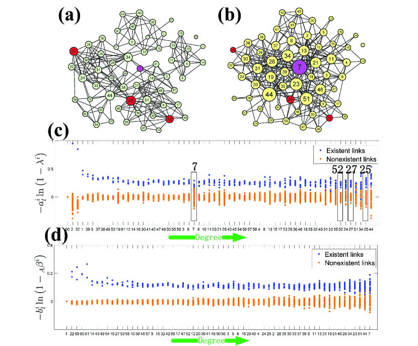
Figure 1: Reconstruction of the CS-AARHUS network. (a) Actual structure of the virtual contact layer (Facebook). (b) The structure of the physical layer. (c,d) The values of $-a_{l}^{i}\ln\left({1-{\lambda^{i}}}\right),~{}i\neq l$ and $-b_{l}^{i}\ln\left({1-{\lambda^{i}}}\right)~{}i\neq l$, respectively, versus the nodal degree. Each column gives the connectivity of a node, where the blue and orange dots denote the existent and nonexistent links, respectively. The length of the time series is $M=30000$. The parameter values for the dynamical processes are $\lambda=0.2$, ${}_{U}{\beta}=0.2$, ${}_{A}{\beta}=0.5{}_{U}{\beta}$, and $\mu=\delta=0.8$.

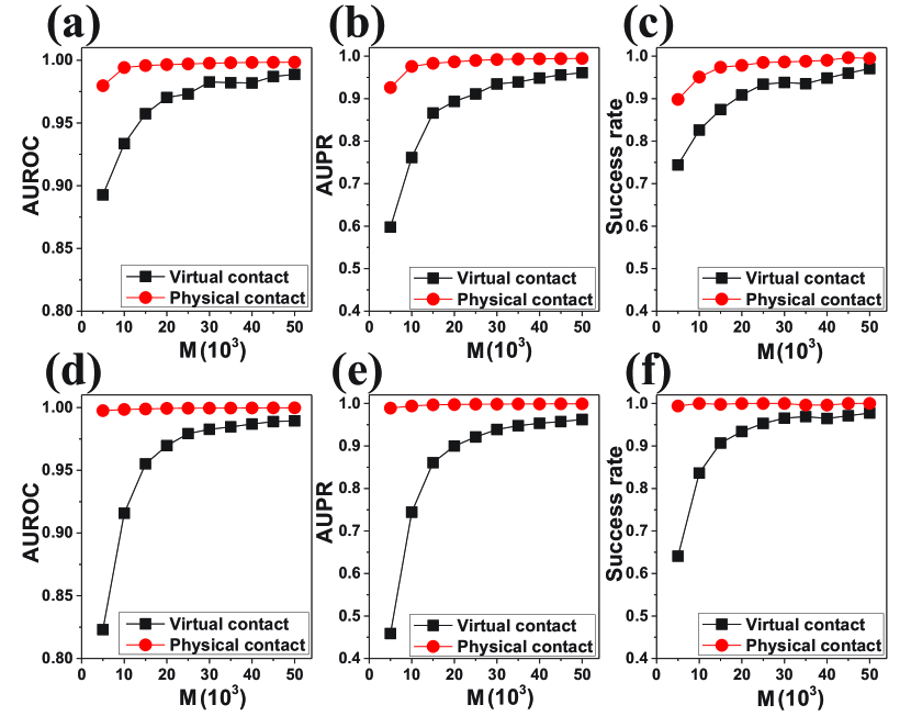
Figure 2: Reconstruction accuracy of C. elegans and CKM networks. (a-c) For the C. elegans network, values of AUROC, AUPR and Success rate versus the length $M$ of the time series, respectively, for the parameter setting $\lambda=0.2$, ${}_{U}{\beta}=0.3$, ${}_{A}{\beta}=0.5{}_{U}{\beta}$, and $\mu=\delta=0.8$. (d-f) The corresponding results for the CKM network for the same parameter values as for (a-c) except ${}_{U}{\beta}=0.5$.

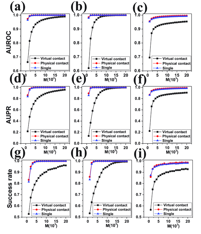
Figure 3: Effect of interlayer coupling on reconstruction accuracy. Columns 1-3: reconstruction performance for ER-ER, SW-SW, and BA-BA duplex networks, respectively. The “single” case indicates the absence of interlayer coupling: ${}_{U}{\beta}=0$ ($\lambda=0$) for the virtual (physical) layer. The parameter setting is $\lambda=0.4$, ${}_{U}{\beta}=0.4$, ${}_{A}{\beta}=0.5{}_{U}{\beta}$, and $\mu=\delta=0.8$. The structures of the two layers are identical. The network parameters are $N=100$ and $\langle k_{1}\rangle=\langle k_{2}\rangle=6$.

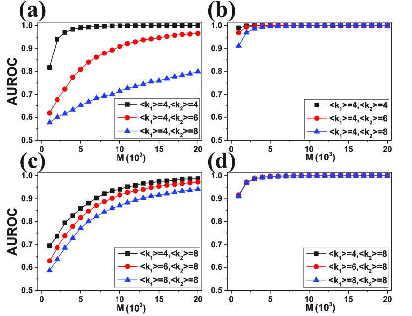
Figure 4: Effect of average degree on reconstruction as measured by the AUROC index. (a,b) For a fixed value of the average degree $\langle k_{1}\rangle$ of the virtual layer, the effect of varying the average degree $\langle k_{2}\rangle$ of the physical layer on the reconstruction accuracy of the former and latter, respectively. (c,d) For a fixed value of $\langle k_{2}\rangle$, the effect of varying the value of $\langle k_{1}\rangle$ on the reconstruction accuracy of the virtual and physical layer, respectively. ER-ER duplex networks with $N$=100 are used. The parameters are $\lambda=0.3$, ${}_{U}{\beta}=0.4$, ${}_{A}{\beta}=0.5{}_{U}{\beta}$, and $\mu=\delta=0.8$.

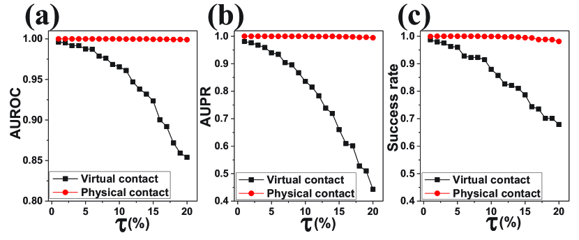
Figure 5: Impact of noise on reconstruction accuracy. (a-c) AUROC, AUPR and Success rate versus the fraction $\tau$ of randomly flipped states for an ER-ER duplex system. The network parameters are $N=100$, $\langle k_{1}\rangle=4$, and $\langle k_{2}\rangle=6$. The length of the time series is $M=30000$. Other parameters are the same as in Fig. 4.

Performance demonstration: reconstruction of three real-world duplex networks.

For a network layer (say the virtual layer), the mathematical formulation of our reconstruction framework gives a characteristic, node-specific quantity for distinguishing the existent from the non-existent links: $-a_{l}^{i}\ln\left({1-{\lambda^{i}}}\right)$, where $\mathbf{a}^{i}$ is the vector defining the local connection structure of node $i$: $a^{i}_{l}=1$ specifies that node $l$ is in the neighborhood of $i$ and $a^{i}_{j}=0$ otherwise, and $\lambda^{i}$ is the probability that node $i$ (if it is unaware) is informed by an aware (A) neighbor. For actual links, the values of $-a_{l}^{i}\ln\left({1-{\lambda^{i}}}\right)$ are finite and away from zero, while the values for non-existent links are near zero. If there is a gap between the two sets of values, the actual links can be detected. A similar quantity can be defined for the physical layer, which is denoted as $-b_{l}^{i}\ln\left(1-{}_{A}\beta\right)$.

We first validate our framework using an empirical network of 61 nodes, the so-called CS-AARHUS network MMR:2013 . The original network has five layers. We regard the Facebook layer as the virtual layer and the other four off-line layers (Leisure, Work, Co-authorship, Lunch) as the physical layer, as illustrated in Figs. 1(a,b), respectively. Figures 1(c,d) show the values of characteristic quantities $-a_{l}^{i}\ln\left({1-{\lambda^{i}}}\right)$ and $-b_{l}^{i}\ln\left(1-{}_{A}\beta\right)$ for the virtual and physical layers, where the blue and orange dots denote the actual and nonexistent links, respectively. We see that the values of the characteristic quantities are well separated by a distinct gap and can be unequivocally distinguished through a properly chosen threshold (see also Fig. 8 in SI). For the physical layer in Fig. 1(d), the gap between the blue and orange dots exhibits a decreasing trend with the nodal degree, indicating that the neighbors of larger degree nodes are harder to be detected because of neighborhood overlapping associated with such nodes. This result is consistent with previous findings SWFDL:2014 ; MZL:2007 . For the virtual layer [Fig. 1(c)], the blue and orange dots for node 7 are overlapped even though ${}^{1}{k^{7}}=6$, but there is a finite gap for large degree nodes, e.g., node 52 with ${}^{1}{k^{52}}=10$, node 27 with ${}^{1}{k^{27}}=12$, and node 25 with ${}^{1}{k^{25}}=15$. The relatively small gap of ${}^{1}{k^{7}}$ is due to the fact that the counterpart value in the physical layer is large: ${}^{2}{k^{7}}=29$, indicating that the node has been infected and is thus constantly in the A state in the virtual layer (an infected node becomes aware immediately). As a result, the states of the neighbors of this node in the virtual layer have little influence on its state, making reconstruction difficult. For nodes with large and small degrees in the virtual and physical layers, respectively, the transition from U to A is mainly determined by the states of the neighbors, facilitating reconstruction. In general, the structure of the physical layer has a significant effect on the reconstruction of the virtual layer, but the effect in the opposite direction is minimal.

We next demonstrate the power of our reconstruction framework for two additional empirical networks: C. elegans DGPA:2016 and the innovation diffusion network for physicians (the so-called CKM network) CKM:1957 . Each network has three layers. We choose the first and the second layer as the virtual and physical layer, respectively. The panels in the top and bottom rows of Fig. 2 display the reconstruction accuracy in terms of the statistical quantities AUROC, AUPR and Success rate (Methods) versus the length of the time series for the C. elegans and CKM networks, respectively. We have that longer time series result in better reconstruction performance and the reconstruction accuracy of the physical layer is higher than that of the virtual layer, which are consistent with the results in Fig. 1.

Performance analysis: reconstruction of synthetic multiplex networks.

To understand the effect of interlayer coupling on reconstruction, we test a number of synthetic complex networks: small-world (SW-SW) WS:1998 , Erdös-Rényi (ER-ER) ER:1960 , and Barabási-Albert (BA-BA) BA:1999 duplex systems. For comparison, we include the special case where each layer is separately reconstructed without taking into account the other layer, which is equivalent to reconstructing a single-layer network (labeled as single). Figures 3(a-i) show that the reconstruction accuracy of the virtual layer is greatly reduced when a physical layer is introduced (e.g., blue/red $\rightarrow$ black). Without the physical layer, the transition of an unaware node in the virtual layer to the aware state depends only on the states of its neighbors. With the presence of the physical layer, an A-node can spontaneously become aware once it is infected, “concealing” the information about the structure of the virtual layer. On the contrary, the reconstruction accuracy of the physical layer can be improved slightly (e.g., blue versus red) when the virtual layer is introduced, which reduces the ability to infect of A-nodes and prevents too many nodes from being in the I state, facilitating reconstruction. Figure  3 also illustrates that the reconstruction accuracy of the SW-SW duplex network is higher than that of the ER-ER duplex network and much higher than that of the BA-BA duplex network due to the difficulty in reconstructing the neighbors of large degree nodes.

How does the average degree of each layer affect the reconstruction accuracy? Figure 4(a) shows that an increase in the average degree $\langle k_{2}\rangle$ of the physical layer can greatly reduce the reconstruction accuracy of the virtual layer. Figures 4(b,c) show that, for the physical layer, the accuracy gradually decreases with its average degree, for a fixed average degree of the virtual layer. An explanation is that the probability of being infected tends to increase for a larger value of $\langle k_{1}\rangle$, “hiding” the information required for uncovering the structure of the virtual layer. We also find that increasing the average degree $\langle k_{1}\rangle$ of the virtual layer tends to reduce the reconstruction accuracy of itself [Fig. 4(c)] but has a negligible effect on the reconstruction of the physical layer [Fig. 4(d)].

Figure 5 shows the effect of noise on the reconstruction accuracy, where noise is implemented by randomly flipping a fraction $\tau$ of the states among the total number $MN$ of states. Noise has a significant effect on the reconstruction of the virtual layer, but it hardly affects the reconstruction of the physical layer (even when the flip rate is $\tau=20\%$).

Discussion

We have developed a mean-field based maximum likelihood estimation framework to solve the challenging problem of data based reconstruction of multiplex networks. The reconstruction performance has been demonstrated using a number of real-world and synthetic duplex networks comprising a virtual and a physical layer, where each layer hosts a distinct type of spreading dynamics that are coupled through the duplex network structure. Extensive test and analysis indicate that the framework is capable of accurately reconstructing the full topology of each layer based solely on measured time series. A thorough examination of the dynamical coupling between the two layers gives that the reconstruction accuracy of the physical layer is generally much higher than that of the virtual layer. In addition, the reconstruction accuracy of the virtual layer is more sensitive to external noise than that of the physical layer.

Our framework represents a starting point towards reconstructing more general multiplex networks hosting different types of dynamics. Appealing features are that the framework is parameter free, has high accuracy, is readily to be implemented, and has a solid mathematical foundation. Issues warranting further considerations include extension to continuous-time dynamical processes, generalization to multiplex networks consisting of more than two layers, and development of effective and practical methods to reduce the required data amount.

Methods

UAU-SIS dynamics on duplex networks.

The UAU-SIS model was originally articulated to study the competition between social awareness and disease spreading on double layer networks, where the physical contact layer supports an epidemic process and the virtual contact layer supports awareness diffusion GGA:2013 . The two layers share exactly the same set of nodes but their connection patterns are different. Spreading of awareness in the virtual layer is described by the classic SIS type of epidemic dynamics: an unaware node (U) is informed by an aware neighbor (A) with probability $\lambda$, and an aware node can lose awareness and returns to the U state with probability $\delta$. Epidemic dynamics in the physical layer are also of the SIS type, where an infected (I) node can infect its susceptible (S) neighbors with probability $\beta$, and an I-node returns to the S state with probability $\mu$. The interlayer interaction is described, as follows. An I-node in the physical layer is automatically aware of the infection and changes to the A state immediately in the virtual layer. If an S-node is in the A state, its ability to infect is reduced by a factor $0\leq\gamma<1$. Figure 6 in SI presents a schematic illustration of the duplex network with the described interacting dynamical process.

Mathematical formulation of the reconstruction framework.

For a duplex network hosting UAU-SIS dynamics, at any time a node can be in one of the three distinct states: unaware and susceptible (US), aware and susceptible (AS), or aware and infected (AI). The state UI (unaware and infected) is redundant because an I-node becomes aware immediately. The connections of node $i$ in the virtual and physical layers are specified by the vectors $\mathbf{a}^{i}$ and $\mathbf{b}^{i}$, respectively, where $a^{i}_{j}=1$ indicates that node $j$ is a neighbor of node $i$ in the virtual layer and $a^{i}_{j}=0$ otherwise, and $b^{i}_{j}$ is defined similarly.

The various transition probabilities can be derived from the transition tree of the UAU-SIS model (Fig. 7 in SI). Let $\sideset{{}_{U}}{}{\mathop{\beta}}$ and $\sideset{{}_{A}}{}{\mathop{\beta}}=\gamma\cdot\sideset{{}_{U}}{}{\mathop{\beta}}$ be the infection rates of unaware and aware S-node, respectively. For node $i$, $\sum\limits_{j\neq i}{a_{j}^{i}~{}{}^{1}s_{t}^{j}}$ and $\sum\limits_{j\neq i}{b_{j}^{i}~{}{}^{2}s_{t}^{j}}$ are the numbers of A-neighbors in the virtual layer and I-neighbors in the physical layer, respectively. The following probabilities are essential to the spreading dynamics: (1) $r_{i}^{t}$, the probability that node $i$ is not informed by any neighbor, (2) ${}_{U}q_{t}^{i}$, the probability that node $i$ is not infected by any neighbor if $i$ was unaware, and (3) ${}_{A}q_{t}^{i}$, the probability that node $i$ is not infected by any neighbor if $i$ was aware. In the absence of any dynamical correlation, these probabilities are given by

$$\begin{array}[]{l}r_{t}^{i}={\left({1-{\lambda^{i}}}\right)^{\sum\limits_{j\neq i}{a_{j}^{i}{}^{1}s_{t}^{j}}}},\\ {}_{U}q_{t}^{i}={\left({1-{}_{U}{\beta^{i}}}\right)^{\sum\limits_{j\neq i}{b_{j}^{i}{}^{2}s_{t}^{j}}}},\\ {}_{A}q_{t}^{i}={\left({1-{}_{A}{\beta^{i}}}\right)^{\sum\limits_{j\neq i}{b_{j}^{i}{}^{2}s_{t}^{j}}}}.\end{array}$$ (4)

A tacit assumption in Ref. GGA:2013 is that diffusion of awareness in the virtual layer occurs before epidemic spreading in the physical layer. In our work, we do not require that the two types of spreading dynamics occur in any particular order.

From Fig. 7 in SI and Eq. (4), we have that the probabilities of node $i$ being in the US, AS and AI states at $t+1$ when it is in the US state at time $t$ are

$$\begin{array}[]{l}P^{US\rightarrow US}=r_{t}^{i}{}_{U}q_{t}^{i},\\ P^{US\rightarrow AS}=\left({1-r_{t}^{i}}\right){}_{U}q_{t}^{i},\\ P^{US\rightarrow AI}=r_{t}^{i}\left({1-{}_{U}q_{t}^{i}}\right)+\left({1-r_{t}^{i}}\right)\left({1-{}_{U}q_{t}^{i}}\right)=1-{}_{U}q_{t}^{i}.\end{array}$$ (8)

The probabilities of node $i$ being in the US, AS and AI states at $t+1$ when it is in the AS state at time $t$ are

$$\begin{array}[]{l}P^{AS\rightarrow US}={\delta^{i}}{}_{A}q_{t}^{i},\\ P^{AS\rightarrow AS}=\left({1-{\delta^{i}}}\right){}_{A}q_{t}^{i},\\ P^{AS\rightarrow AI}={\delta^{i}}\left({1-{}_{A}q_{t}^{i}}\right)+\left({1-{\delta^{i}}}\right)\left({1-{}_{A}q_{t}^{i}}\right)=1-{}_{A}q_{t}^{i}.\end{array}$$ (12)

The probabilities for node $i$ to be in the US, AS and AI states at $t+1$ if it is in the AI state at time $t$ are

$$\begin{array}[]{l}P^{AI\rightarrow US}={\delta^{i}}{\mu^{i}},\\ P^{AI\rightarrow AS}=\left({1-{\delta^{i}}}\right){\mu^{i}},\\ P^{AI\rightarrow AI}=1-{\mu^{i}}.\end{array}$$ (16)

Say only the states ${}^{1}s_{t_{m}}^{i}$ and ${}^{2}s_{t_{m}}^{i}$ ($i=1,\ldots,N$) at time $t_{m}$ (not necessarily uniform) are recorded, where $N$ is the network size. Our framework consists of three steps: (1) to reconstruct the likelihood function of the coupled dynamics, (2) to apply the mean-field approximation to enable maximum likelihood estimation (MLE), and (3) to transform the MLE problem into two solvable linear systems - one for each layer with solutions representing the neighbors of each node in the layer. In particular, the likelihood function of node $i$ is given by (see Sec. III of SI):

$$\begin{array}[]{l}\quad P\left({{{\left\{{{}^{1}s_{{t_{m}}+1}^{i},{}^{2}s_{{t_{m}}+1}^{i}}\right\}}_{m=1\cdots M}}|{{\left\{{{}^{1}s_{{t_{m}}}^{j},{}^{2}s_{{t_{m}}}^{j}}\right\}}_{j=1\cdots N,m=1\cdots M}},{\mathbf{a}^{i}},{\mathbf{b}^{i}},{\lambda^{i}},{}_{U}{\beta^{i}},{}_{A}{\beta^{i}},{\delta^{i}},{\mu^{i}}}\right)\\ ={\prod\limits_{m}{\left[{{{\left({r_{{t_{m}}}^{i}{}_{U}q_{{t_{m}}}^{i}}\right)}^{\left({1-{}^{1}s_{{t_{m}}+1}^{i}}\right)\left({1-{}^{2}s_{{t_{m}}+1}^{i}}\right)}}{{\left({\left({1-r_{{t_{m}}}^{i}}\right){}_{U}q_{{t_{m}}}^{i}}\right)}^{{}^{1}s_{{t_{m}}+1}^{i}\left({1-{}^{2}s_{{t_{m}}+1}^{i}}\right)}}{{\left({1-{}_{U}q_{{t_{m}}}^{i}}\right)}^{{}^{1}s_{{t_{m}}+1}^{i}{}^{2}s_{{t_{m}}+1}^{i}}}}\right]}^{\left({1-{}^{1}s_{{t_{m}}}^{i}}\right)\left({1-{}^{2}s_{{t_{m}}}^{i}}\right)}}\\ \quad\quad{\left[{{{\left({{\delta^{i}}{}_{A}q_{{t_{m}}}^{i}}\right)}^{\left({1-{}^{1}s_{{t_{m}}+1}^{i}}\right)\left({1-{}^{2}s_{{t_{m}}+1}^{i}}\right)}}{{\left({\left({1-{\delta^{i}}}\right){}_{A}q_{{t_{m}}}^{i}}\right)}^{{}^{1}s_{{t_{m}}+1}^{i}\left({1-{}^{2}s_{{t_{m}}+1}^{i}}\right)}}{{\left({1-{}_{A}q_{{t_{m}}}^{i}}\right)}^{{}^{1}s_{{t_{m}}+1}^{i}{}^{2}s_{{t_{m}}+1}^{i}}}}\right]^{{}^{1}s_{{t_{m}}}^{i}\left({1-{}^{2}s_{{t_{m}}}^{i}}\right)}}\\ \quad\quad{\left[{{{\left({{\delta^{i}}{\mu^{i}}}\right)}^{\left({1-{}^{1}s_{{t_{m}}+1}^{i}}\right)\left({1-{}^{2}s_{{t_{m}}+1}^{i}}\right)}}{{\left({\left({1-{\delta^{i}}}\right){\mu^{i}}}\right)}^{{}^{1}s_{{t_{m}}+1}^{i}\left({1-{}^{2}s_{{t_{m}}+1}^{i}}\right)}}{{\left({1-{\mu^{i}}}\right)}^{{}^{1}s_{{t_{m}}+1}^{i}{}^{2}s_{{t_{m}}+1}^{i}}}}\right]^{{}^{1}s_{{t_{m}}}^{i}{}^{2}s_{{t_{m}}}^{i}}},\end{array}$$ (21)

where $M$ is the length of the time series (step 1). The logarithmic form of Eq. (21), denoted as

$$L=L\left({{a^{i}},{b^{i}},{\lambda^{i}},{}_{U}{\beta^{i}},{}_{A}{\beta^{i}},{\delta^{i}},{\mu^{i}}}\right),$$

can be written as

$$L={L_{0}}\left({{\delta^{i}},{\mu^{i}}}\right)+{L_{1}}\left({{\mathbf{a^{i}}},{\lambda^{i}}}\right)+{L_{2}}\left({{\mathbf{b^{i}}},{}_{U}{\beta^{i}},{}_{A}{\beta^{i}}}\right).$$

MLE can be performed by maximizing $L_{0}$, $L_{1}$ and $L_{2}$ (Sec. III of SI). Because $L_{0}$ does not contain information about the network structure, it is only necessary to maximize $L_{1}$ and $L_{2}$ with respect to $a^{i}_{j}$ and $b^{i}_{j}$, respectively. The likelihood function for reconstructing the virtual layer is (see Sec. III of SI for the corresponding function for the physical layer):

$${L_{1}}\left({{\mathbf{a^{i}}},{\lambda^{i}}}\right)=\sum\limits_{m}{}^{1}X_{{t_{m}}}^{i}\ln\left({{{\left({1-{\lambda^{i}}}\right)}^{\sum\limits_{j\neq i}{a_{j}^{i}{}^{1}s_{{t_{m}}}^{j}}}}}\right)+\sum\limits_{m}{}^{1}Y_{{t_{m}}}^{i}\ln\left({1-{{\left({1-{\lambda^{i}}}\right)}^{\sum\limits_{j\neq i}{a_{j}^{i}{}^{1}s_{{t_{m}}}^{j}}}}}\right)$$ (22)

where

$${}^{1}X_{{t_{m}}}^{i} = \left({1-{}^{1}s_{{t_{m}}}^{i}}\right)\left({1-{}^{1}s_{{t_{m}}+1}^{i}}\right)\ \mbox{and}$$

$${}^{1}Y_{{t_{m}}}^{i} = \left({1-{}^{1}s_{{t_{m}}}^{i}}\right)\left({1-{}^{2}s_{{t_{m}}+1}^{i}}\right){}^{1}s_{{t_{m}}+1}^{i}.$$

The maximum value of $L_{1}$ cannot be obtained straightforwardly by setting zero its derivative with respect to $a_{j}^{i}$, because $a_{j}^{i}$ appears in the exponential term and the values of $\lambda^{i}$ are unknown. We resort to the mean-field approximation to solve this problem (step 2). Specifically, for node $i$ in the virtual layer, the fraction $\sum\limits_{j\neq i}{{}^{1}s_{{t_{m}}}^{j}a_{j}^{i}}$ of A-neighbors is approximately equal to the fraction of A-nodes in the whole layer excluding node $i$ itself:

$$\sum\limits_{j\neq i}{{}^{1}s_{{t_{m}}}^{j}a_{j}^{i}}\approx\frac{{{}^{1}{k^{i}}}}{{N-1}}{}^{1}\theta_{{t_{m}}}^{i},$$ (23)

where ${}^{1}{k^{i}}$ is the degree of node $i$, ${}^{1}\theta_{{t_{m}}}^{i}=\sum\limits_{j\neq i}{{}^{1}s_{{t_{m}}}^{j}}$ is the number of A-nodes excluding node $i$ itself. Letting

$${}^{1}{\gamma^{i}}={\left({1-{\lambda^{i}}}\right)^{\frac{{{}^{1}{k^{i}}}}{{N-1}}}},$$

we rewrite Eq. (22) concisely as

$${\hat{L}_{1}}\left({{}^{1}{\gamma^{i}}}\right)=\sum\limits_{m}{\left[\begin{array}[]{l}{}^{1}X_{{t_{m}}}^{i}\ln\left({{{\left({{}^{1}{\gamma^{i}}}\right)}^{{}^{1}\theta_{{t_{m}}}^{i}}}}\right)+{}^{1}Y_{{t_{m}}}^{i}\ln\left({1-{{\left({{}^{1}{\gamma^{i}}}\right)}^{{}^{1}\theta_{{t_{m}}}^{i}}}}\right)\end{array}\right]}.$$ (25)

Differentiating $\hat{L}_{1}\left({}^{1}{\gamma^{i}}\right)$ with respect to ${}^{1}{\gamma^{i}}$ and setting it to zero, we get the equation

$$\sum\limits_{m}{{}^{1}Y_{{t_{m}}}^{i}{}^{1}\theta_{{t_{m}}}^{i}\frac{{{{\left({{}^{1}{\gamma^{i}}}\right)}^{{}^{1}\theta_{{t_{m}}}^{i}}}}}{{1-{{\left({{}^{1}{\gamma^{i}}}\right)}^{{}^{1}\theta_{{t_{m}}}^{i}}}}}}=\sum\limits_{m}{{}^{1}X_{{t_{m}}}^{i}{}^{1}\theta_{{t_{m}}}^{i}},$$ (26)

whose solutions give the values of ${}^{1}{\gamma^{i}}$ denoted as ${}^{1}{\gamma^{i}}={}^{1}{\tilde{\gamma}^{i}}$.

To transform the MLE problem into a linear system (step 3), we take the derivative of Eq. (22) with respect to $a^{i}_{l}$ and set it to zero, which gives the following high-dimensional nonlinear equation (the detailed reconstruction process for the virtual and physical layers is given in Secs. IV and V of SI, respectively):

$$\sum\limits_{m}{{}^{1}Y_{{t_{m}}}^{i}{}^{1}s_{{t_{m}}}^{l}\frac{{{{\left({1-{\lambda^{i}}}\right)}^{\sum\limits_{j\neq i}{a_{j}^{i}~{}{}^{1}s_{{t_{m}}}^{j}}}}}}{{1-{{\left({1-{\lambda^{i}}}\right)}^{\sum\limits_{j\neq i}{a_{j}^{i}~{}{}^{1}s_{{t_{m}}}^{j}}}}}}}=\sum\limits_{m}{{}^{1}X_{{t_{m}}}^{i}{}^{1}s_{{t_{m}}}^{l}}.$$

To obtain a solution, we take advantage of Eq. (23) and use the first-order approximation. The result is a solvable linear system expressed in the matrix form

$$\bm{\Lambda}\cdot\bm{\eta}=\bm{\zeta},$$ (27)

with the vector

$$\bm{\eta}=\big{[}{a_{1}^{i}\ln\left({1-{\lambda^{i}}}\right)},\ldots,{a_{i-1}^{i}\ln\left({1-{\lambda^{i}}}\right)},{a_{i+1}^{i}\ln\left({1-{\lambda^{i}}}\right)},\ldots,{a_{N}^{i}\ln\left({1-{\lambda^{i}}}\right)}\big{]}^{T}$$

(see Sec. IV of SI for the detailed forms of $\bm{\Lambda}$ and $\bm{\zeta}$). With the available time series ${}^{1}s_{t_{m}}^{i}$ and ${}^{2}s_{t_{m}}^{i}$, the values of the elements of the matrix $\bm{\Lambda}$ and the components of the vector $\bm{\zeta}$ can be calculated, so that the vector $\bm{\eta}$ characterizing the connectivity of node $i$ can be solved. Because $\ln{(1-\lambda^{i})}<0$ is a constant, the value of $-a_{l}^{i}\ln\left({1-{\lambda^{i}}}\right)$ is much above zero for $a^{i}_{l}=1$ or close to zero for $a^{i}_{l}=0$. A threshold value can then be readily set to distinguish the existent from the nonexistent links: a pair of nodes $i$ and $l$ are connected in the virtual layer if the value of $-a_{l}^{i}\ln\left({1-{\lambda^{i}}}\right)$ is larger than the threshold (see Sec. VI in SI for the criterion to choose the threshold).

Evaluation metrics.

We use three metrics LSWGL:2017 to characterize the performance of our reconstruction framework: the area under the receiver operating characteristic curve (AUROC), the area under the precision-recall curve (AUPR), and the Success rate.

To define AUROC and AUPR, it is necessary to calculate three basic quantities: TPR (true positive rate), FPR (false positive rate), and Recall LSWGL:2017 . In particular, TPR is defined as

$$\mbox{TPR}(l)=\frac{\mbox{TP}(l)}{T},$$ (28)

where $l$ is the cut-off index in the list of the predicted links, $\mbox{TP}(l)$ is the number of true positives in the top $l$ predictions in the link list, and $T$ is the number of positives.

FPR is defined as

$$\mbox{FPR}(l)=\frac{\mbox{FP}(l)}{Q},$$ (29)

where $\mbox{FP}(l)$ is the number of false positives in the top $l$ entries in the predicted link list, and $Q$ is the number of negatives by the golden standard.

Recall and Precision are defined as

$$\mbox{Recall}(l)=\mbox{TPR}(l)=\frac{\mbox{TP}(l)}{T}.$$ (30)

and

$$\mbox{Precision}(l)=\frac{\mbox{TP}(l)}{\mbox{TP}(l)+\mbox{FP}(l)}=\frac{\mbox{TP}(l)}{l},$$ (31)

respectively. Varying the value of $l$ from $0$ to $N$, we plot two sequences of points: [$\mbox{FPR}(l)$, $\mbox{TPR}(l)$] and [$\mbox{Recall}(l)$, $\mbox{Precision}(l)$]. The area under the two curves correspond to the values of AUROC and AUPR, respectively. For perfect reconstruction, we have AUROC=1 and AUPR=1. In the worst case (completely random), we have AUROC=0.5 and AUPR=$T/2N$.

Let $n_{1}$ and $n_{2}$ be the numbers of the actual and nonexistent links in the network, respectively, $n_{3}$ and $n_{4}$ be the numbers of the predicted existent and nonexistent links. The Success rates for actual links (SREL) and nonexistent links (SRNL) are defined as $n_{3}/n_{1}$ and $n_{4}/n_{2}$, respectively. The normalized Success rate is $\sqrt{\mbox{SQEL}\times\mbox{SRNL}}$ SWFDL:2014 .

Contents

1. I UAU-SIS dynamics on multiplex networks with a double-layer structure
2. II Transition tree of UAU-SIS model
3. III Likelihood function
4. IV Reconstruction of virtual layer
5. V Reconstruction of physical layer
6. VI Selection of threshold value for identification of existent links
7. VII Reconstruction of duplex networks with heterogeneous rates of spreading dynamics

I UAU-SIS dynamics on multiplex networks with a double-layer structure

The UAU-SIS model was originally articulated to describe the competition between social awareness and disease spreading on double layer networks, where the physical contact layer supports an epidemic process and the virtual contact layer supports awareness diffusion GGA:2013 . The two layers share exactly the same set of nodes but their connection patterns are different. Spreading of awareness in the virtual layer is described by the conventional SIS dynamics: an unaware node (U) is informed by an aware neighbor (A) with probability $\lambda$, and an aware node can lose awareness and returns to the U state with probability $\delta$. Epidemic dynamics in the physical layer are also of the SIS type, where an infected (I) node can infect its susceptible (S) neighbors with probability $\beta$, and an I-node returns to the S state with probability $\mu$. There is interlayer interaction, which can be described, as follows. An I-node in the physical layer is automatically aware of the infection and changes to the A state immediately in the virtual layer. If an S-node is in the A state, its ability to infect is reduced by a factor $0\leq\gamma<1$. Figure 6 presents a schematic illustration of the double layer network with the described interacting dynamical processes.

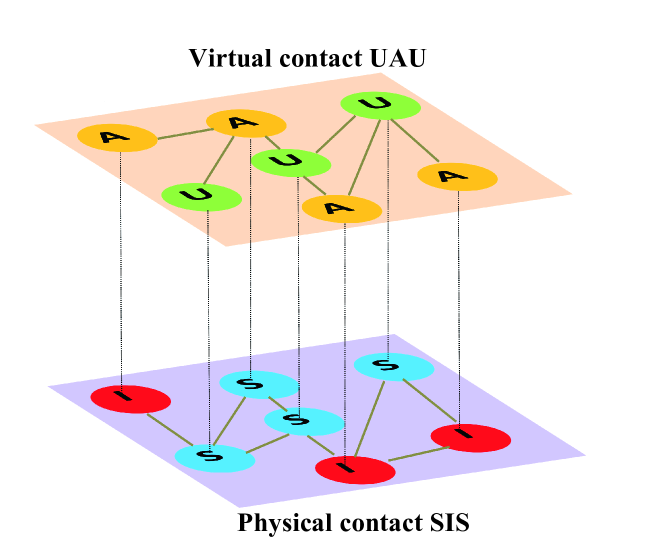
Figure 6: Schematic illustration a multiplex network with a double layer interacting structure. The upper layer (virtual contact) supports awareness diffusion, where each node has two possible states: unaware (U) or aware (A). The bottom layer (physical contact) hosts epidemic spreading dynamics, where a node can be in the susceptible (S) or infected (I) state.

II Transition tree of UAU-SIS model

Let $\sideset{{}_{U}}{}{\mathop{\beta}}$ and $\sideset{{}_{A}}{}{\mathop{\beta}}=\gamma\cdot\sideset{{}_{U}}{}{\mathop{\beta}}$ be the infection rates of unaware and aware S-node, respectively. For node $i$, $\sum\limits_{j\neq i}{a_{j}^{i}~{}{}^{1}s_{t}^{j}}$ and $\sum\limits_{j\neq i}{b_{j}^{i}~{}{}^{2}s_{t}^{j}}$ are the numbers of A-neighbors in the virtual layer and I-neighbors in the physical layer, respectively. Three probabilities are needed to describe the network spreading dynamics: (1) $r_{i}^{t}$, the probability that node $i$ is not informed by any neighbor, (2) ${}_{U}q_{t}^{i}$, the probability that node $i$ is not infected by any neighbor if $i$ was unaware, and (3) ${}_{A}q_{t}^{i}$, the probability that node $i$ is not infected by any neighbor if $i$ was aware. In the absence of any dynamical correlation, the three probabilities are given by

$$\begin{array}[]{l}r_{t}^{i}={\left({1-{\lambda^{i}}}\right)^{\sum\limits_{j\neq i}{a_{j}^{i}{}^{1}s_{t}^{j}}}},\\ {}_{U}q_{t}^{i}={\left({1-{}_{U}{\beta^{i}}}\right)^{\sum\limits_{j\neq i}{b_{j}^{i}{}^{2}s_{t}^{j}}}},\\ {}_{A}q_{t}^{i}={\left({1-{}_{A}{\beta^{i}}}\right)^{\sum\limits_{j\neq i}{b_{j}^{i}{}^{2}s_{t}^{j}}}}.\end{array}$$ (35)

A tacit assumption in Ref. GGA:2013 is that diffusion of awareness in the virtual layer occurs before epidemic spreading in the physical layer. In our work, we do not require that the two types of spreading dynamics occur in any particular order. Figure 7 presents the transition probability tree of the UAU-SIS coupling dynamics on the duplex networks.

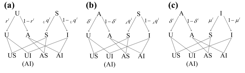
Figure 7: Transition probability tree of coupled UAU-SIS dynamics on duplex networks. The notations are: AI - aware and infected, UI - unaware and infected (redundant to the AI state), AS - aware and susceptible, and US - unaware and susceptible.

From Fig. 7 and Eq. (35), we have that the probabilities of node $i$ being in the US, AS and AI states at $t+1$ when it is in the US state at time $t$ are

$$\begin{array}[]{l}P^{US\rightarrow US}=r_{t}^{i}{}_{U}q_{t}^{i},\\ P^{US\rightarrow AS}=\left({1-r_{t}^{i}}\right){}_{U}q_{t}^{i},\\ P^{US\rightarrow AI}=r_{t}^{i}\left({1-{}_{U}q_{t}^{i}}\right)+\left({1-r_{t}^{i}}\right)\left({1-{}_{U}q_{t}^{i}}\right)=1-{}_{U}q_{t}^{i}.\end{array}$$ (39)

The probabilities of node $i$ being in the US, AS and AI states at $t+1$ when it is in the AS state at time $t$ are

$$\begin{array}[]{l}P^{AS\rightarrow US}={\delta^{i}}{}_{A}q_{t}^{i},\\ P^{AS\rightarrow AS}=\left({1-{\delta^{i}}}\right){}_{A}q_{t}^{i},\\ P^{AS\rightarrow AI}={\delta^{i}}\left({1-{}_{A}q_{t}^{i}}\right)+\left({1-{\delta^{i}}}\right)\left({1-{}_{A}q_{t}^{i}}\right)=1-{}_{A}q_{t}^{i}.\end{array}$$ (43)

The probabilities for node $i$ to be in the US, AS and AI states at $t+1$ if it is in the AI state at time $t$ are

$$\begin{array}[]{l}P^{AI\rightarrow US}={\delta^{i}}{\mu^{i}},\\ P^{AI\rightarrow AS}=\left({1-{\delta^{i}}}\right){\mu^{i}},\\ P^{AI\rightarrow AI}=1-{\mu^{i}}.\end{array}$$ (47)

III Likelihood function

The likelihood function of a node can be written in the following compact form:

$$\quad P\left({{{\left\{{{}^{1}s_{{t_{m}}+1}^{i},{}^{2}s_{{t_{m}}+1}^{i}}\right\}}_{m=1\cdots M}}|{{\left\{{{}^{1}s_{{t_{m}}}^{j},{}^{2}s_{{t_{m}}}^{j}}\right\}}_{j=1\cdots N,m=1\cdots M}},{\mathbf{a}^{i}},{\mathbf{b}^{i}},{\lambda^{i}},{}_{U}{\beta^{i}},{}_{A}{\beta^{i}},{\delta^{i}},{\mu^{i}}}\right)$$

$$= {\prod\limits_{m}{\left[{{{\left({r_{{t_{m}}}^{i}{}_{U}q_{{t_{m}}}^{i}}\right)}^{\left({1-{}^{1}s_{{t_{m}}+1}^{i}}\right)\left({1-{}^{2}s_{{t_{m}}+1}^{i}}\right)}}{{\left({\left({1-r_{{t_{m}}}^{i}}\right){}_{U}q_{{t_{m}}}^{i}}\right)}^{{}^{1}s_{{t_{m}}+1}^{i}\left({1-{}^{2}s_{{t_{m}}+1}^{i}}\right)}}{{\left({1-{}_{U}q_{{t_{m}}}^{i}}\right)}^{{}^{1}s_{{t_{m}}+1}^{i}{}^{2}s_{{t_{m}}+1}^{i}}}}\right]}^{\left({1-{}^{1}s_{{t_{m}}}^{i}}\right)\left({1-{}^{2}s_{{t_{m}}}^{i}}\right)}}$$

$$\quad\quad{\left[{{{\left({{\delta^{i}}{}_{A}q_{{t_{m}}}^{i}}\right)}^{\left({1-{}^{1}s_{{t_{m}}+1}^{i}}\right)\left({1-{}^{2}s_{{t_{m}}+1}^{i}}\right)}}{{\left({\left({1-{\delta^{i}}}\right){}_{A}q_{{t_{m}}}^{i}}\right)}^{{}^{1}s_{{t_{m}}+1}^{i}\left({1-{}^{2}s_{{t_{m}}+1}^{i}}\right)}}{{\left({1-{}_{A}q_{{t_{m}}}^{i}}\right)}^{{}^{1}s_{{t_{m}}+1}^{i}{}^{2}s_{{t_{m}}+1}^{i}}}}\right]^{{}^{1}s_{{t_{m}}}^{i}\left({1-{}^{2}s_{{t_{m}}}^{i}}\right)}}$$

$$\quad\quad{\left[{{{\left({{\delta^{i}}{\mu^{i}}}\right)}^{\left({1-{}^{1}s_{{t_{m}}+1}^{i}}\right)\left({1-{}^{2}s_{{t_{m}}+1}^{i}}\right)}}{{\left({\left({1-{\delta^{i}}}\right){\mu^{i}}}\right)}^{{}^{1}s_{{t_{m}}+1}^{i}\left({1-{}^{2}s_{{t_{m}}+1}^{i}}\right)}}{{\left({1-{\mu^{i}}}\right)}^{{}^{1}s_{{t_{m}}+1}^{i}{}^{2}s_{{t_{m}}+1}^{i}}}}\right]^{{}^{1}s_{{t_{m}}}^{i}{}^{2}s_{{t_{m}}}^{i}}}.$$

In the UAU-SIS model, we assume that a node, once it is infected in the physical layer, enters into the A state immediately in the virtual layer: ${}^{2}s_{{t}}^{i}=1$ indicates ${}^{1}s_{{t}}^{i}=1$ at any time $t$. As a result, we have ${}^{1}s_{{t_{m}}}^{i}{}^{2}s_{{t_{m}}}^{i}={}^{2}s_{{t_{m}}}^{i}$ and ${}^{1}s_{{t_{m}}+1}^{i}{}^{2}s_{{t_{m}}+1}^{i}={}^{2}s_{{t_{m}}+1}^{i}$. Note that a node in the U state in the virtual layer cannot be in the I state in the physical layer, i.e., ${}^{1}s_{{t}}^{i}=0$ indicates ${}^{2}s_{{t}}^{i}=0$ at any time $t$, which leads to

$$\left({1-{}^{1}s_{{t_{m}}}^{i}}\right)\left({1-{}^{2}s_{{t_{m}}}^{i}}\right) = 1-{}^{1}s_{{t_{m}}}^{i}$$

$$\left({1-{}^{1}s_{{t_{m}}+1}^{i}}\right)\left({1-{}^{2}s_{{t_{m}}+1}^{i}}\right) = 1-{}^{1}s_{{t_{m}}+1}^{i}.$$

Equation (III) appears complicated, but it can be reduced to some simple form. For example, assuming that node $i$ at $t_{m}$ is in the US state: ${}^{1}s_{{t_{m}}}^{i}=0$ and ${}^{2}s_{{t_{m}}}^{i}=0$, we need to retain only one term in the product:

$${\left[{{{\left({r_{{t_{m}}}^{i}{}_{U}q_{{t_{m}}}^{i}}\right)}^{\left({1-{}^{1}s_{{t_{m}}+1}^{i}}\right)\left({1-{}^{2}s_{{t_{m}}+1}^{i}}\right)}}{{\left({\left({1-r_{{t_{m}}}^{i}}\right){}_{U}q_{{t_{m}}}^{i}}\right)}^{{}^{1}s_{{t_{m}}+1}^{i}\left({1-{}^{2}s_{{t_{m}}+1}^{i}}\right)}}{{\left({1-{}_{U}q_{{t_{m}}}^{i}}\right)}^{{}^{1}s_{{t_{m}}+1}^{i}{}^{2}s_{{t_{m}}+1}^{i}}}}\right]},$$

which can be further reduced to ${\left({1-r_{{t_{m}}}^{i}}\right){}_{U}q_{{t_{m}}}^{i}}$ if ${}^{1}s_{{t_{m}+1}}^{i}=1$ and ${}^{2}s_{{t_{m}+1}}^{i}=0$ (i.e., in the AS state at the next time step). This corresponds to the transition probability from the US state to the AS state:

$$P^{US\rightarrow AS}=\left({1-r_{t}^{i}}\right){}_{U}q_{t}^{i}$$

in Eq. (39). In general, Eq. (III) contains all the transition probabilities in Eqs. (39)-(47).

After some algebra, we obtain the logarithmic form of Eq. (III) as

$$L\left({{\mathbf{a^{i}}},{\mathbf{b^{i}}},{\lambda^{i}},{}_{U}{\beta^{i}},{}_{A}{\beta^{i}},{\delta^{i}},{\mu^{i}}}\right)={L_{0}}\left({{\delta^{i}},{\mu^{i}}}\right)+{L_{1}}\left({{\mathbf{a^{i}}},{\lambda^{i}}}\right)+{L_{2}}\left({{\mathbf{b^{i}}},{}_{U}{\beta^{i}},{}_{A}{\beta^{i}}}\right),$$ (49)

where

$${L_{0}}\left({{\delta^{i}},{\mu^{i}}}\right)=\sum\limits_{m}{\left[\begin{array}[]{l}{}^{1}s_{{t_{m}}}^{i}\left({1-{}^{1}s_{{t_{m}}+1}^{i}}\right)\ln\left({{\delta^{i}}}\right)+{}^{1}s_{{t_{m}}}^{i}{}^{1}s_{{t_{m}}+1}^{i}\left({1-{}^{2}s_{{t_{m}}+1}^{i}}\right)\ln\left({1-{\delta^{i}}}\right)\\ +{}^{2}s_{{t_{m}}}^{i}\left({1-{}^{2}s_{{t_{m}}+1}^{i}}\right)\ln\left({{\mu^{i}}}\right)+{}^{2}s_{{t_{m}}}^{i}{}^{2}s_{{t_{m}}+1}^{i}\ln\left({1-{\mu^{i}}}\right)\end{array}\right]}.$$ (52)

Note that Eq. (52) does not rely on any information about the network structure. The quantity that does contain the information is ${L_{1}}\left({{a^{i}},{\lambda^{i}}}\right)$, which depends on the connectivity of node $i$ in the virtual layer. It can be written as

$${L_{1}}\left({{\mathbf{a^{i}}},{\lambda^{i}}}\right)=\sum\limits_{m}{\left[{{}^{1}X_{{t_{m}}}^{i}\ln\left({{{\left({1-{\lambda^{i}}}\right)}^{\sum\limits_{j\neq i}{a_{j}^{i}{}^{1}s_{{t_{m}}}^{j}}}}}\right)+{}^{1}Y_{{t_{m}}}^{i}\ln\left({1-{{\left({1-{\lambda^{i}}}\right)}^{\sum\limits_{j\neq i}{a_{j}^{i}{}^{1}s_{{t_{m}}}^{j}}}}}\right)}\right]},$$ (53)

where

$${}^{1}X_{{t_{m}}}^{i} = \left({1-{}^{1}s_{{t_{m}}}^{i}}\right)\left({1-{}^{1}s_{{t_{m}}+1}^{i}}\right)\ \ \mbox{and}$$

$${}^{1}Y_{{t_{m}}}^{i} = \left({1-{}^{1}s_{{t_{m}}}^{i}}\right)\left({1-{}^{2}s_{{t_{m}}+1}^{i}}\right){}^{1}s_{{t_{m}}+1}^{i}.$$

Similarly, the quantity ${L_{2}}\left({{b^{i}},{}_{U}{\beta^{i}},{}_{A}{\beta^{i}}}\right)$ that depends on the connectivity of node $i$ in the physical layer is given by

$${L_{2}}\left({{\mathbf{b^{i}}},{}_{U}{\beta^{i}},{}_{A}{\beta^{i}}}\right)=$$

$$\sum\limits_{m}\left[{{}_{U}^{2}X_{{t_{m}}}^{i}\ln\left({{{\left({1-{}_{U}{\beta^{i}}}\right)}^{\sum\limits_{j\neq i}{b_{j}^{i}{}^{2}s_{{t_{m}}}^{j}}}}}\right)+{}_{U}^{2}Y_{{t_{m}}}^{i}\ln\left({1-{{\left({1-{}_{U}{\beta^{i}}}\right)}^{\sum\limits_{j\neq i}{b_{j}^{i}{}^{2}s_{{t_{m}}}^{j}}}}}\right)}\right]$$

$$+ \sum\limits_{m}\left[{{}_{A}^{2}X_{{t_{m}}}^{i}\ln\left({{{\left({1-{}_{A}{\beta^{i}}}\right)}^{\sum\limits_{j\neq i}{b_{j}^{i}{}^{2}s_{{t_{m}}}^{j}}}}}\right)+{}_{A}^{2}Y_{{t_{m}}}^{i}\ln\left({1-{{\left({1-{}_{A}{\beta^{i}}}\right)}^{\sum\limits_{j\neq i}{b_{j}^{i}{}^{2}s_{{t_{m}}}^{j}}}}}\right)}\right]$$

where

$${}_{U}^{2}X_{{t_{m}}}^{i} = \left({1-{}^{1}s_{{t_{m}}}^{i}}\right)\left({1-{}^{2}s_{{t_{m}}+1}^{i}}\right),$$

$${}_{U}^{2}Y_{{t_{m}}}^{i} = \left({1-{}^{1}s_{{t_{m}}}^{i}}\right){}^{2}s_{{t_{m}}+1}^{i},$$

$${}_{A}^{2}X_{{t_{m}}}^{i} = {}^{1}s_{{t_{m}}}^{i}\left({1-{}^{2}s_{{t_{m}}}^{i}}\right)\left({1-{}^{2}s_{{t_{m}}+1}^{i}}\right),\ \ \mbox{and}$$

$${}_{A}^{2}Y_{{t_{m}}}^{i} = {}^{1}s_{{t_{m}}}^{i}\left({1-{}^{2}s_{{t_{m}}}^{i}}\right){}^{2}s_{{t_{m}}+1}^{i}.$$

In principle, Eq. (49) indicates that one can maximize $L_{1}$ and $L_{2}$ with respect to $a^{i}_{j}$ and $b^{i}_{j}$, respectively, to uncover the connectivity of node $i$. However, the conventional maximization process leads to equations that cannot be solved because the quantity $a_{j}^{i}$ ($b_{j}^{i}$) appears in the exponential term and the values of $\lambda^{i}$ (or ${}_{U}{\beta^{i}}$) are unknown. We exploit the mean-field approximation to maximize $L_{1}$ and $L_{2}$.

IV Reconstruction of virtual layer

To infer the neighbors of node $i$ in the virtual layer, we impose the mean-field approximation on $L_{1}$:

$$\sum\limits_{j\neq i}{{}^{1}s_{{t_{m}}}^{j}a_{j}^{i}}\approx\frac{{{}^{1}{k^{i}}}}{{N-1}}{}^{1}\theta_{{t_{m}}}^{i},$$ (55)

where $N$ and ${}^{1}{k^{i}}$ are the number of nodes and the degree of node $i$ in the virtual layer, respectively, and the number of A-nodes in the virtual layer (excluding node $i$ itself) is ${}^{1}\theta_{{t_{m}}}^{i}=\sum\limits_{j\neq i}{{}^{1}s_{{t_{m}}}^{j}}$. A new unknown parameter ${}^{1}{k^{i}}$ emerges in Eq. (53) when we substitute Eq. (55) into Eq. (53). To simplify the analysis, we let

$${}^{1}{\gamma^{i}}={\left({1-{\lambda^{i}}}\right)^{\frac{{{}^{1}{k^{i}}}}{{N-1}}}},$$ (56)

to obtain

$${\left({1-{\lambda^{i}}}\right)^{\sum\limits_{j\neq i}{a_{j}^{i}~{}{}^{1}s_{{t_{m}}}^{j}}}}={\left({1-{\lambda^{i}}}\right)^{\frac{{{}^{1}{k^{i}}}}{{N-1}}{}^{1}\theta_{{t_{m}}}^{i}}}={\left({{}^{1}{\gamma^{i}}}\right)^{{}^{1}\theta_{{t_{m}}}^{i}}}.$$

Equation (53) can then be written concisely as

$${\hat{L}_{1}}\left({{}^{1}{\gamma^{i}}}\right)=\sum\limits_{m}{\left[\begin{array}[]{l}{}^{1}X_{{t_{m}}}^{i}\ln\left({{{\left({{}^{1}{\gamma^{i}}}\right)}^{{}^{1}\theta_{{t_{m}}}^{i}}}}\right)+{}^{1}Y_{{t_{m}}}^{i}\ln\left({1-{{\left({{}^{1}{\gamma^{i}}}\right)}^{{}^{1}\theta_{{t_{m}}}^{i}}}}\right)\end{array}\right]}.$$ (58)

Differentiating $\hat{L}_{1}\left({}^{1}{\gamma^{i}}\right)$ with respect to ${}^{1}{\gamma^{i}}$ and setting it to zero, we get

$$\sum\limits_{m}{{}^{1}Y_{{t_{m}}}^{i}{}^{1}\theta_{{t_{m}}}^{i}\frac{{{{\left({{}^{1}{\gamma^{i}}}\right)}^{{}^{1}\theta_{{t_{m}}}^{i}}}}}{{1-{{\left({{}^{1}{\gamma^{i}}}\right)}^{{}^{1}\theta_{{t_{m}}}^{i}}}}}}=\sum\limits_{m}{{}^{1}X_{{t_{m}}}^{i}{}^{1}\theta_{{t_{m}}}^{i}},$$

leading to ${}^{1}{\gamma^{i}}={}^{1}{\tilde{\gamma}^{i}}$.

Treating $a^{i}_{l}$ as a continuous variance, we can further differentiate Eq. (53) with respect to $a^{i}_{l}$ and set it to zero, which gives

$$\sum\limits_{m}{{}^{1}Y_{{t_{m}}}^{i}~{}{}^{1}s_{{t_{m}}}^{l}\frac{{{{\left({1-{\lambda^{i}}}\right)}^{\sum\limits_{j\neq i}{a_{j}^{i}~{}{}^{1}s_{{t_{m}}}^{j}}}}}}{{1-{{\left({1-{\lambda^{i}}}\right)}^{\sum\limits_{j\neq i}{a_{j}^{i}{}^{1}s_{{t_{m}}}^{j}}}}}}}=\sum\limits_{m}{{}^{1}X_{{t_{m}}}^{i}{}^{1}s_{{t_{m}}}^{l}}.$$ (59)

To obtain analytical solutions of Eq. (59) is not feasible due to its nonlinear and high-dimensional nature. We thus resort to the first-order Taylor expansion. In particular, we expand $a^{x}/(1-a^{x})$ in the limit $x\rightarrow x_{0}$ to obtain

$$\frac{{{a^{x}}}}{{1-{a^{x}}}}\approx\frac{{{a^{{x_{0}}}}}}{{1-{a^{{x_{0}}}}}}+\frac{{{a^{{x_{0}}}}\ln a}}{{{{\left({1-{a^{{x_{0}}}}}\right)}^{2}}}}\left({x-{x_{0}}}\right)=\frac{{{a^{{x_{0}}}}}}{{1-{a^{{x_{0}}}}}}-\frac{{{a^{{x_{0}}}}\ln{a^{{x_{0}}}}}}{{{{\left({1-{a^{{x_{0}}}}}\right)}^{2}}}}+\frac{{{a^{{x_{0}}}}\ln a}}{{{{\left({1-{a^{{x_{0}}}}}\right)}^{2}}}}x.$$ (60)

Setting $x=\sum\limits_{j\neq i}{a_{j}^{i}~{}{}^{1}s_{{t_{m}}}^{j}}$, $a=1-{\lambda^{i}}$, and ${x_{0}}=\frac{{{}^{1}{k^{i}}}}{{N-1}}{}^{1}\theta_{{t_{m}}}^{i}$ [Eq. (55) implies that $x\approx x_{0}$], we have

$${a^{{x_{0}}}}={\left({{}^{1}{{\tilde{\gamma}}^{i}}}\right)^{{}^{1}\theta_{{t_{m}}}^{i}}}$$

from Eq. (56). That is, the term

$${\frac{{{{\left({1-{\lambda^{i}}}\right)}^{\sum\limits_{j\neq i}{a_{j}^{i}~{}{}^{1}s_{{t_{m}}}^{j}}}}}}{{1-{{\left({1-{\lambda^{i}}}\right)}^{\sum\limits_{j\neq i}{a_{j}^{i}~{}{}^{1}s_{{t_{m}}}^{j}}}}}}}$$

in Eq. (59) can be expressed as a linear form based on Eq. (55.)

Collecting all the approximations, we transform Eq. (59) into a solvable linear system as

$$\begin{array}[]{l}\sum\limits_{m}{{}^{1}Y_{{t_{m}}}^{i}{}^{1}G_{{t_{m}}}^{i}{}^{1}s_{{t_{m}}}^{l}\ln\left({1-{\lambda^{i}}}\right)\sum\limits_{j\neq i}{a_{j}^{i}~{}{}^{1}s_{{t_{m}}}^{j}}}=\sum\limits_{m}{\left({{}^{1}X_{{t_{m}}}^{i}-{}^{1}Y_{{t_{m}}}^{i}{}^{1}F_{{t_{m}}}^{i}}\right)~{}{}^{1}s_{{t_{m}}}^{l}},\end{array}$$ (62)

where

$${}^{1}F_{{t_{m}}}^{i} = \frac{{{{\left({{}^{1}{{\tilde{\gamma}}^{i}}}\right)}^{{}^{1}\theta_{{t_{m}}}^{i}}}}}{{1-{{\left({{}^{1}{{\tilde{\gamma}}^{i}}}\right)}^{{}^{1}\theta_{{t_{m}}}^{i}}}}}-\frac{{{{\left({{}^{1}{{\tilde{\gamma}}^{i}}}\right)}^{{}^{1}\theta_{{t_{m}}}^{i}}}}}{{{{\left({1-{{\left({{}^{1}{{\tilde{\gamma}}^{i}}}\right)}^{{}^{1}\theta_{{t_{m}}}^{i}}}}\right)}^{2}}}}{}^{1}\theta_{{t_{m}}}^{i}\ln{}^{1}{\tilde{\gamma}^{i}}\ \ \mbox{and}$$

$${}^{1}G_{{t_{m}}}^{i} = \frac{{{{\left({{}^{1}{{\tilde{\gamma}}^{i}}}\right)}^{{}^{1}\theta_{{t_{m}}}^{i}}}}}{{{{\left({1-{{\left({{}^{1}{{\tilde{\gamma}}^{i}}}\right)}^{{}^{1}\theta_{{t_{m}}}^{i}}}}\right)}^{2}}}}.$$

Setting ${}^{1}\Phi_{{t_{m}}}^{i}={}^{1}Y_{{t_{m}}}^{i}{}^{1}G_{{t_{m}}}^{i}$ and ${}^{1}\Gamma_{{t_{m}}}^{i}$ = ${}^{1}X_{{t_{m}}}^{i}-{}^{1}Y_{{t_{m}}}^{i}{}^{1}F_{{t_{m}}}^{i}$, we express Eq. (62) as

$$\left[{\begin{array}[]{*{20}{c}}{\sum\limits_{m}{{}^{1}\Phi_{{t_{m}}}^{i}{}^{1}s_{{t_{m}}}^{1}{}^{1}s_{{t_{m}}}^{1}}}&\cdots&{\sum\limits_{m}{{}^{1}\Phi_{{t_{m}}}^{i}{}^{1}s_{{t_{m}}}^{1}{}^{1}s_{{t_{m}}}^{i-1}}}&{\sum\limits_{m}{{}^{1}\Phi_{{t_{m}}}^{i}{}^{1}s_{{t_{m}}}^{1}{}^{1}s_{{t_{m}}}^{i+1}}}&\cdots&{\sum\limits_{m}{{}^{1}\Phi_{{t_{m}}}^{i}{}^{1}s_{{t_{m}}}^{1}{}^{1}s_{{t_{m}}}^{N}}}\\ \vdots&{}\hfil&\vdots&\vdots&{}\hfil&\vdots\\ {\sum\limits_{m}{{}^{1}\Phi_{{t_{m}}}^{i}{}^{1}s_{{t_{m}}}^{i-1}{}^{1}s_{{t_{m}}}^{1}}}&\cdots&{\sum\limits_{m}{{}^{1}\Phi_{{t_{m}}}^{i}{}^{1}s_{{t_{m}}}^{i-1}{}^{1}s_{{t_{m}}}^{i-1}}}&{\sum\limits_{m}{{}^{1}\Phi_{{t_{m}}}^{i}{}^{1}s_{{t_{m}}}^{i-1}{}^{1}s_{{t_{m}}}^{i+1}}}&\cdots&{\sum\limits_{m}{{}^{1}\Phi_{{t_{m}}}^{i}{}^{1}s_{{t_{m}}}^{i-1}{}^{1}s_{{t_{m}}}^{N}}}\\ {\sum\limits_{m}{{}^{1}\Phi_{{t_{m}}}^{i}{}^{1}s_{{t_{m}}}^{i+1}{}^{1}s_{{t_{m}}}^{1}}}&\cdots&{\sum\limits_{m}{{}^{1}\Phi_{{t_{m}}}^{i}{}^{1}s_{{t_{m}}}^{i+1}{}^{1}s_{{t_{m}}}^{i-1}}}&{\sum\limits_{m}{{}^{1}\Phi_{{t_{m}}}^{i}{}^{1}s_{{t_{m}}}^{i+1}{}^{1}s_{{t_{m}}}^{i+1}}}&\cdots&{\sum\limits_{m}{{}^{1}\Phi_{{t_{m}}}^{i}{}^{1}s_{{t_{m}}}^{i+1}{}^{1}s_{{t_{m}}}^{N}}}\\ \vdots&{}\hfil&\vdots&\vdots&{}\hfil&\vdots\\ {\sum\limits_{m}{{}^{1}\Phi_{{t_{m}}}^{i}{}^{1}s_{{t_{m}}}^{N}{}^{1}s_{{t_{m}}}^{1}}}&\cdots&{\sum\limits_{m}{{}^{1}\Phi_{{t_{m}}}^{i}{}^{1}s_{{t_{m}}}^{N}{}^{1}s_{{t_{m}}}^{i-1}}}&{\sum\limits_{m}{{}^{1}\Phi_{{t_{m}}}^{i}{}^{1}s_{{t_{m}}}^{N}{}^{1}s_{{t_{m}}}^{i+1}}}&\cdots&{\sum\limits_{m}{{}^{1}\Phi_{{t_{m}}}^{i}{}^{1}s_{{t_{m}}}^{N}{}^{1}s_{{t_{m}}}^{N}}}\end{array}}\right]$$ (69)

$$\times \left[{\begin{array}[]{*{20}{c}}{a_{1}^{i}\ln\left({1-{\lambda^{i}}}\right)}\\ \vdots\\ {a_{i-1}^{i}\ln\left({1-{\lambda^{i}}}\right)}\\ {a_{i+1}^{i}\ln\left({1-{\lambda^{i}}}\right)}\\ \vdots\\ {a_{N}^{i}\ln\left({1-{\lambda^{i}}}\right)}\end{array}}\right]=\left[{\begin{array}[]{*{20}{c}}{\sum\limits_{m}{{}^{1}\Gamma_{{t_{m}}}^{i}{}^{1}s_{{t_{m}}}^{1}}}\\ \vdots\\ {\sum\limits_{m}{{}^{1}\Gamma_{{t_{m}}}^{i}{}^{1}s_{{t_{m}}}^{i-1}}}\\ {\sum\limits_{m}{{}^{1}\Gamma_{{t_{m}}}^{i}{}^{1}s_{{t_{m}}}^{i+1}}}\\ \vdots\\ {\sum\limits_{m}{{}^{1}\Gamma_{{t_{m}}}^{i}{}^{1}s_{{t_{m}}}^{N}}}\end{array}}\right].$$ (82)

The matrix on the left side (labeled as $\bm{\Lambda}$) and the vector (labeled as $\mathbf{\bm{\zeta}}$) on the right side of Eq. (69) can be calculated from the time series of the nodal states. The vector

$$\bm{\eta}=\big{[}{a_{1}^{i}\ln\left({1-{\lambda^{i}}}\right)},\ldots,{a_{i-1}^{i}\ln\left({1-{\lambda^{i}}}\right)},{a_{i+1}^{i}\ln\left({1-{\lambda^{i}}}\right)},\ldots,{a_{N}^{i}\ln\left({1-{\lambda^{i}}}\right)}\big{]}^{T}$$

can then be solved, where $T$ denotes transpose. Note that the quantity $\ln\left({1-{\lambda^{i}}}\right)<0$ is a constant even though $\lambda^{i}$ is not given, implying that the value of $-a_{j}^{i}\ln\left({1-{\lambda^{i}}}\right)$ is positively large for $a^{i}_{j}=1$ and near zero for $a^{i}_{j}=0$. As a result, the neighbors of node $i$ in the virtual layer can be ascertained through the solution of the vector $\bm{\eta}$.

V Reconstruction of physical layer

The mean-field approximation for the physical layer is

$$\sum\limits_{j\neq i}{{}^{2}s_{{t_{m}}}^{j}b_{j}^{i}}\approx\frac{{{}^{2}{k^{i}}}}{{N-1}}{}^{2}\theta_{{t_{m}}}^{i},$$ (83)

where ${}^{2}{k^{i}}$ is the degree of node $i$ and ${}^{2}\theta_{{t_{m}}}^{i}=\sum\limits_{j\neq i}{{}^{2}s_{{t_{m}}}^{j}}$ is the number of I-nodes in the physical layer (excluding node $i$ itself). We set

$$\begin{array}[]{l}{}_{U}^{2}{\gamma^{i}}={\left({1-{}_{U}{\beta^{i}}}\right)^{\frac{{{}^{2}{k^{i}}}}{{N-1}}}}\ \mbox{and}\\ {}_{A}^{2}{\gamma^{i}}={\left({1-{}_{A}{\beta^{i}}}\right)^{\frac{{{}^{2}{k^{i}}}}{{N-1}}}}\end{array}$$ (86)

and write Eq. (III) concisely as

$${\hat{L}_{2}}\left({{}_{U}^{2}{\gamma^{i}},{}_{A}^{2}{\gamma^{i}}}\right)=\sum\limits_{m}{\left\{\begin{array}[]{l}\left[{{}_{U}^{2}X_{{t_{m}}}^{i}\ln\left({{{\left({{}_{U}^{2}{\gamma^{i}}}\right)}^{~{}{}^{2}\theta_{{t_{m}}}^{i}}}}\right)+{}_{U}^{2}Y_{{t_{m}}}^{i}\ln\left({1-{{\left({{}_{U}^{2}{\gamma^{i}}}\right)}^{~{}{}^{2}\theta_{{t_{m}}}^{i}}}}\right)}\right]\\ +\left[{{}_{A}^{2}X_{{t_{m}}}^{i}\ln\left({{{\left({{}_{A}^{2}{\gamma^{i}}}\right)}^{~{}{}^{2}\theta_{{t_{m}}}^{i}}}}\right)+{}_{A}^{2}Y_{{t_{m}}}^{i}\ln\left({1-{{\left({{}_{A}^{2}{\gamma^{i}}}\right)}^{~{}{}^{2}\theta_{{t_{m}}}^{i}}}}\right)}\right]\end{array}\right\}}.$$ (89)

Taking the derivatives of $\hat{L}_{2}$ with respect to ${}_{U}^{2}{\gamma^{i}}$ and ${}_{A}^{2}{\gamma^{i}}$ and setting them to zero, we get

$$\sum\limits_{m}{{}_{U}^{2}Y_{{t_{m}}}^{i}~{}{}^{2}\theta_{{t_{m}}}^{i}\frac{{{{\left({{}_{U}^{2}{\gamma^{i}}}\right)}^{~{}{}^{2}\theta_{{t_{m}}}^{i}}}}}{{1-{{\left({{}_{U}^{2}{\gamma^{i}}}\right)}^{~{}{}^{2}\theta_{{t_{m}}}^{i}}}}}}=\sum\limits_{m}{{}_{U}^{2}X_{{t_{m}}}^{i}~{}{}^{2}\theta_{{t_{m}}}^{i}}$$ (90)

and

$$\sum\limits_{m}{{}_{A}^{2}Y_{{t_{m}}}^{i}~{}{}^{2}\theta_{{t_{m}}}^{i}\frac{{{{\left({{}_{A}^{2}{\gamma^{i}}}\right)}^{~{}{}^{2}\theta_{{t_{m}}}^{i}}}}}{{1-{{\left({{}_{A}^{2}{\gamma^{i}}}\right)}^{{}^{2}\theta_{{t_{m}}}^{i}}}}}}=\sum\limits_{m}{{}_{A}^{2}X_{{t_{m}}}^{i}~{}{}^{2}\theta_{{t_{m}}}^{i}}\emph{},$$ (91)

which give

$${}_{U}^{2}{\gamma^{i}} = {}_{U}^{2}{\tilde{\gamma}^{i}}\ \mbox{and}$$

$${}_{A}^{2}{\gamma^{i}} = {}_{A}^{2}{\tilde{\gamma}^{i}}.$$

Similar to the mean-field analysis of the virtual layer, we differentiate Eq. (III) with respect to $b_{l}^{i}$ and set it to zero:

$$\frac{{\partial{L_{2}}}}{{\partial b_{l}^{i}}} = \sum\limits_{m}\left[{\ln\left({1-{}_{U}{\beta^{i}}}\right){}_{U}^{2}X_{{t_{m}}}^{i}~{}{}^{2}s_{{t_{m}}}^{l}-\ln\left({1-{}_{U}{\beta^{i}}}\right){}_{U}^{2}Y_{{t_{m}}}^{i}~{}{}^{2}s_{{t_{m}}}^{l}\frac{{{{\left({1-{}_{U}{\beta^{i}}}\right)}^{\sum\limits_{j\neq i}{b_{j}^{i}~{}{}^{2}s_{{t_{m}}}^{j}}}}}}{{1-{{\left({1-{}_{U}{\beta^{i}}}\right)}^{\sum\limits_{j\neq i}{b_{j}^{i}~{}{}^{2}s_{{t_{m}}}^{j}}}}}}}\right]$$

$$+ \sum\limits_{m}\left[{\ln\left({1-{}_{A}{\beta^{i}}}\right){}_{A}^{2}X_{{t_{m}}}^{i}~{}{}^{2}s_{{t_{m}}}^{l}-\ln\left({1-{}_{A}{\beta^{i}}}\right){}_{A}^{2}Y_{{t_{m}}}^{i}~{}{}^{2}s_{{t_{m}}}^{l}\frac{{{{\left({1-{}_{A}{\beta^{i}}}\right)}^{\sum\limits_{j\neq i}{b_{j}^{i}~{}{}^{2}s_{{t_{m}}}^{j}}}}}}{{1-{{\left({1-{}_{A}{\beta^{i}}}\right)}^{\sum\limits_{j\neq i}{b_{j}^{i}~{}{}^{2}s_{{t_{m}}}^{j}}}}}}}\right]=0,$$

which gives

$$\sum\limits_{m}{\left\{{\ln\left({1-{}_{U}{\beta^{i}}}\right)~{}{}^{2}s_{{t_{m}}}^{l}{}_{U}^{2}Y_{{t_{m}}}^{i}\frac{{{{\left({1-{}_{U}{\beta^{i}}}\right)}^{\sum\limits_{j\neq i}{b_{j}^{i}~{}{}^{2}s_{{t_{m}}}^{j}}}}}}{{1-{{\left({1-{}_{U}{\beta^{i}}}\right)}^{\sum\limits_{j\neq i}{b_{j}^{i}~{}{}^{2}s_{{t_{m}}}^{j}}}}}}+\ln\left({1-{}_{A}{\beta^{i}}}\right){}^{2}s_{{t_{m}}}^{l}{}_{A}^{2}Y_{{t_{m}}}^{i}\frac{{{{\left({1-{}_{A}{\beta^{i}}}\right)}^{\sum\limits_{j\neq i}{b_{j}^{i}{}^{2}s_{{t_{m}}}^{j}}}}}}{{1-{{\left({1-{}_{A}{\beta^{i}}}\right)}^{\sum\limits_{j\neq i}{b_{j}^{i}~{}{}^{2}s_{{t_{m}}}^{j}}}}}}}\right\}}$$ (92)

$$= \sum\limits_{m}{\left\{{\ln\left({1-{}_{U}{\beta^{i}}}\right){}_{U}^{2}X_{{t_{m}}}^{i}~{}{}^{2}s_{{t_{m}}}^{l}+\ln\left({1-{}_{A}{\beta^{i}}}\right){}_{A}^{2}X_{{t_{m}}}^{i}{}^{2}s_{{t_{m}}}^{l}}\right\}}.$$

Setting

$$\rho=\frac{{\ln{}_{U}^{2}{{\tilde{\gamma}}^{i}}}}{{\ln{}_{A}^{2}{{\tilde{\gamma}}^{i}}}}=\frac{{\ln\left({1-{}_{U}{\beta^{i}}}\right)}}{{\ln\left({1-{}_{A}{\beta^{i}}}\right)}},$$

we can further simplify Eq. (92) as

$$\begin{array}[]{l}\sum\limits_{m}{\left[{\rho~{}~{}{{}^{2}s_{{t_{m}}}^{l}}~{}{}_{U}^{2}Y_{{t_{m}}}^{i}\frac{{{{\left({1-{}_{U}{\beta^{i}}}\right)}^{\sum\limits_{j\neq i}{b_{j}^{i}~{}{}^{2}s_{{t_{m}}}^{j}}}}}}{{1-{{\left({1-{}_{U}{\beta^{i}}}\right)}^{\sum\limits_{j\neq i}{b_{j}^{i}{}^{2}s_{{t_{m}}}^{j}}}}}}+{}^{2}s_{{t_{m}}}^{l}{}_{A}^{2}Y_{{t_{m}}}^{i}\frac{{{{\left({1-{}_{A}{\beta^{i}}}\right)}^{\sum\limits_{j\neq i}{b_{j}^{i}{}^{2}s_{{t_{m}}}^{j}}}}}}{{1-{{\left({1-{}_{A}{\beta^{i}}}\right)}^{\sum\limits_{j\neq i}{b_{j}^{i}{}^{2}s_{{t_{m}}}^{j}}}}}}}\right]}\\ =\sum\limits_{m}{\left[{\rho~{}~{}{}_{U}^{2}X_{{t_{m}}}^{i}{}^{2}s_{{t_{m}}}^{l}+{}_{A}^{2}X_{{t_{m}}}^{i}{}^{2}s_{{t_{m}}}^{l}}\right]}\end{array}$$ (95)

Using Eq. (60) and setting $x=\sum\limits_{j\neq i}{b_{j}^{i}~{}{}^{2}s_{{t_{m}}}^{j}}$ and ${x_{0}}=\frac{{{}^{2}{k^{i}}}}{{N-1}}{}^{2}\theta_{{t_{m}}}^{i}$, we obtain the following Taylor expansion:

$$\frac{{{{\left({1-{}_{U}{\beta^{i}}}\right)}^{\sum\limits_{j\neq i}{b_{j}^{i}~{}{}^{2}s_{{t_{m}}}^{j}}}}}}{{1-{{\left({1-{}_{U}{\beta^{i}}}\right)}^{\sum\limits_{j\neq i}{b_{j}^{i}~{}{}^{2}s_{{t_{m}}}^{j}}}}}}={}_{U}^{2}F_{{t_{m}}}^{i}+{}_{U}^{2}G_{{t_{m}}}^{i}\ln\left({1-{}_{U}{\beta^{i}}}\right)\sum\limits_{j\neq i}{b_{j}^{i}~{}{}^{2}s_{{t_{m}}}^{j}},$$ (96)

where

$${}_{U}^{2}F_{{t_{m}}}^{i} = \frac{{{{\left({{}_{U}^{2}{{\tilde{\gamma}}^{i}}}\right)}^{~{}{}^{2}\theta_{{t_{m}}}^{i}}}}}{{1-{{\left({{}_{U}^{2}{{\tilde{\gamma}}^{i}}}\right)}^{~{}{}^{2}\theta_{{t_{m}}}^{i}}}}}-\frac{{{{\left({{}_{U}^{2}{{\tilde{\gamma}}^{i}}}\right)}^{~{}{}^{2}\theta_{{t_{m}}}^{i}}}}}{{{{\left({1-{{\left({{}_{U}^{2}{{\tilde{\gamma}}^{i}}}\right)}^{~{}{}^{2}\theta_{{t_{m}}}^{i}}}}\right)}^{2}}}}~{}{}^{2}\theta_{{t_{m}}}^{i}\ln{}_{U}^{2}{\tilde{\gamma}^{i}}\ \mbox{and}$$

$${}_{U}^{2}G_{{t_{m}}}^{i} = \frac{{{{\left({{}_{U}^{2}{{\tilde{\gamma}}^{i}}}\right)}^{~{}{}^{2}\theta_{{t_{m}}}^{i}}}}}{{{{\left({1-{{\left({{}_{U}^{2}{{\tilde{\gamma}}^{i}}}\right)}^{~{}{}^{2}\theta_{{t_{m}}}^{i}}}}\right)}^{2}}}}.$$

We also have

$$\frac{{{{\left({1-{}_{A}{\beta^{i}}}\right)}^{\sum\limits_{j\neq i}{b_{j}^{i}~{}{}^{2}s_{{t_{m}}}^{j}}}}}}{{1-{{\left({1-{}_{A}{\beta^{i}}}\right)}^{\sum\limits_{j\neq i}{b_{j}^{i}~{}{}^{2}s_{{t_{m}}}^{j}}}}}}={}_{A}^{2}F_{{t_{m}}}^{i}+{}_{A}^{2}G_{{t_{m}}}^{i}\ln\left({1-{}_{A}{\beta^{i}}}\right)\sum\limits_{j\neq i}{b_{j}^{i}~{}{}^{2}s_{{t_{m}}}^{j}},$$ (97)

where

$${}_{A}^{2}F_{{t_{m}}}^{i} = \frac{{{{\left({{}_{A}^{2}{{\tilde{\gamma}}^{i}}}\right)}^{~{}{}^{2}\theta_{{t_{m}}}^{i}}}}}{{1-{{\left({{}_{A}^{2}{{\tilde{\gamma}}^{i}}}\right)}^{~{}{}^{2}\theta_{{t_{m}}}^{i}}}}}-\frac{{{{\left({{}_{A}^{2}{{\tilde{\gamma}}^{i}}}\right)}^{~{}{}^{2}\theta_{{t_{m}}}^{i}}}}}{{{{\left({1-{{\left({{}_{A}^{2}{{\tilde{\gamma}}^{i}}}\right)}^{~{}{}^{2}\theta_{{t_{m}}}^{i}}}}\right)}^{2}}}}{}^{2}\theta_{{t_{m}}}^{i}\ln{}_{A}^{2}{\tilde{\gamma}^{i}}\ \mbox{and}$$

$${}_{A}^{2}G_{{t_{m}}}^{i} = \frac{{{{\left({{}_{A}^{2}{{\tilde{\gamma}}^{i}}}\right)}^{~{}{}^{2}\theta_{{t_{m}}}^{i}}}}}{{{{\left({1-{{\left({{}_{A}^{2}{{\tilde{\gamma}}^{i}}}\right)}^{~{}{}^{2}\theta_{{t_{m}}}^{i}}}}\right)}^{2}}}}.$$

With these approximations, we can transform Eq. (95) into the following linear system:

$$\begin{array}[]{l}\sum\limits_{m}{\left[{\left({{\rho^{2}}~{}{}_{U}^{2}Y_{{t_{m}}}^{i}~{}{}_{U}^{2}G_{{t_{m}}}^{i}+{}_{A}^{2}Y_{{t_{m}}}^{i}~{}{}_{A}^{2}G_{{t_{m}}}^{i}}\right)~{}{}^{2}s_{{t_{m}}}^{l}\ln\left({1-{}_{A}{\beta^{i}}}\right)\sum\limits_{j\neq i}{b_{j}^{i}~{}{}^{2}s_{{t_{m}}}^{j}}}\right]}\\ =\sum\limits_{m}{\left({\rho~{}{}_{U}^{2}X_{{t_{m}}}^{i}+{}_{A}^{2}X_{{t_{m}}}^{i}-\rho~{}{}_{U}^{2}Y_{{t_{m}}}^{i}~{}{}_{U}^{2}F_{{t_{m}}}^{i}-{}_{A}^{2}Y_{{t_{m}}}^{i}~{}{}_{A}^{2}F_{{t_{m}}}^{i}}\right)}~{}{}^{2}s_{{t_{m}}}^{l},\end{array}$$ (100)

where

$${}^{2}\Phi_{{t_{m}}}^{i} = {\rho^{2}}~{}{}_{U}^{2}Y_{{t_{m}}}^{i}~{}{}_{U}^{2}G_{{t_{m}}}^{i}+{}_{A}^{2}Y_{{t_{m}}}^{i}~{}{}_{A}^{2}G_{{t_{m}}}^{i}\ \mbox{and}$$

$${}^{2}\Gamma_{{t_{m}}}^{i} = \rho~{}{}_{U}^{2}X_{{t_{m}}}^{i}+{}_{A}^{2}X_{{t_{m}}}^{i}-\rho~{}{}_{U}^{2}Y_{{t_{m}}}^{i}~{}{}_{U}^{2}F_{{t_{m}}}^{i}-{}_{A}^{2}Y_{{t_{m}}}^{i}~{}{}_{A}^{2}F_{{t_{m}}}^{i}.$$

We rewrite Eq. (100) in the following matrix form:

$$\left[{\begin{array}[]{*{20}{c}}{\sum\limits_{m}{{}^{2}\Phi_{{t_{m}}}^{i}{}^{2}s_{{t_{m}}}^{1}{}^{2}s_{{t_{m}}}^{1}}}&\cdots&{\sum\limits_{m}{{}^{2}\Phi_{{t_{m}}}^{i}{}^{2}s_{{t_{m}}}^{1}{}^{2}s_{{t_{m}}}^{i-1}}}&{\sum\limits_{m}{{}^{2}\Phi_{{t_{m}}}^{i}{}^{2}s_{{t_{m}}}^{1}{}^{2}s_{{t_{m}}}^{i+1}}}&\cdots&{\sum\limits_{m}{{}^{2}\Phi_{{t_{m}}}^{i}{}^{2}s_{{t_{m}}}^{1}{}^{2}s_{{t_{m}}}^{N}}}\\ \vdots&{}\hfil&\vdots&\vdots&{}\hfil&\vdots\\ {\sum\limits_{m}{{}^{2}\Phi_{{t_{m}}}^{i}{}^{2}s_{{t_{m}}}^{i-1}{}^{2}s_{{t_{m}}}^{1}}}&\cdots&{\sum\limits_{m}{{}^{2}\Phi_{{t_{m}}}^{i}{}^{2}s_{{t_{m}}}^{i-1}{}^{2}s_{{t_{m}}}^{i-1}}}&{\sum\limits_{m}{{}^{2}\Phi_{{t_{m}}}^{i}{}^{2}s_{{t_{m}}}^{i-1}{}^{2}s_{{t_{m}}}^{i+1}}}&\cdots&{\sum\limits_{m}{{}^{2}\Phi_{{t_{m}}}^{i}{}^{2}s_{{t_{m}}}^{i-1}{}^{2}s_{{t_{m}}}^{N}}}\\ {\sum\limits_{m}{{}^{2}\Phi_{{t_{m}}}^{i}{}^{2}s_{{t_{m}}}^{i+1}{}^{2}s_{{t_{m}}}^{1}}}&\cdots&{\sum\limits_{m}{{}^{2}\Phi_{{t_{m}}}^{i}{}^{2}s_{{t_{m}}}^{i+1}{}^{2}s_{{t_{m}}}^{i-1}}}&{\sum\limits_{m}{{}^{2}\Phi_{{t_{m}}}^{i}{}^{2}s_{{t_{m}}}^{i+1}{}^{2}s_{{t_{m}}}^{i+1}}}&\cdots&{\sum\limits_{m}{{}^{2}\Phi_{{t_{m}}}^{i}{}^{2}s_{{t_{m}}}^{i+1}{}^{2}s_{{t_{m}}}^{N}}}\\ \vdots&{}\hfil&\vdots&\vdots&{}\hfil&\vdots\\ {\sum\limits_{m}{{}^{2}\Phi_{{t_{m}}}^{i}{}^{2}s_{{t_{m}}}^{N}{}^{2}s_{{t_{m}}}^{1}}}&\cdots&{\sum\limits_{m}{{}^{2}\Phi_{{t_{m}}}^{i}{}^{2}s_{{t_{m}}}^{N}{}^{2}s_{{t_{m}}}^{i-1}}}&{\sum\limits_{m}{{}^{2}\Phi_{{t_{m}}}^{i}{}^{2}s_{{t_{m}}}^{N}{}^{2}s_{{t_{m}}}^{i+1}}}&\cdots&{\sum\limits_{m}{{}^{2}\Phi_{{t_{m}}}^{i}{}^{2}s_{{t_{m}}}^{N}{}^{2}s_{{t_{m}}}^{N}}}\end{array}}\right]$$ (107)

$$\times \left[{\begin{array}[]{*{20}{c}}{b_{1}^{i}\ln\left({1-{}_{A}{\beta^{i}}}\right)}\\ \vdots\\ {b_{i-1}^{i}\ln\left({1-{}_{A}{\beta^{i}}}\right)}\\ {b_{i+1}^{i}\ln\left({1-{}_{A}{\beta^{i}}}\right)}\\ \vdots\\ {b_{N}^{i}\ln\left({1-{}_{A}{\beta^{i}}}\right)}\end{array}}\right]=\left[{\begin{array}[]{*{20}{c}}{\sum\limits_{m}{{}^{2}\Gamma_{{t_{m}}}^{i}{}^{2}s_{{t_{m}}}^{1}}}\\ \vdots\\ {\sum\limits_{m}{{}^{2}\Gamma_{{t_{m}}}^{i}{}^{2}s_{{t_{m}}}^{i-1}}}\\ {\sum\limits_{m}{{}^{2}\Gamma_{{t_{m}}}^{i}{}^{2}s_{{t_{m}}}^{i+1}}}\\ \vdots\\ {\sum\limits_{m}{{}^{2}\Gamma_{{t_{m}}}^{i}{}^{2}s_{{t_{m}}}^{N}}}\end{array}}\right].$$ (120)

The matrix on the left side and the vector on the right side can be obtained from time series. Solution of Eq. (107) gives the vector

$$\bm{\eta}=\big{[}b_{1}^{i}\ln\left({1-{}_{A}{\beta^{i}}}\right),\ldots,b_{i-1}^{i}\ln\left({1-{}_{A}{\beta^{i}}}\right),b_{i+1}^{i}\ln\left({1-{}_{A}{\beta^{i}}}\right),\ldots,b_{N}^{i}\ln\left({1-{}_{A}{\beta^{i}}}\right)\big{]}^{T},$$

revealing the neighbors of node $i$ in the physical layer.

VI Selection of threshold value for identification of existent links

For each node $i$, the values of $a_{l}^{i}\ln\left({1-{\lambda^{i}}}\right)$ (or of $b_{l}^{i}\ln\left({1-{}_{A}{\beta^{i}}}\right)$) can be obtained from Eq. (69) [or Eq. (107)]. From Figs. 8(a,b), we have that the values of $-a_{l}^{i}\ln\left({1-{\lambda^{i}}}\right)$ [or $-b_{l}^{i}\ln\left({1-{}_{A}{\beta^{i}}}\right)$] are unequivocally above zero for the actual links, while their values are close to zero for nonexistent links, with a gap between the two sets of values. Representing the values listed in each column as a histogram, we have that the peak centered about zero corresponds to nonexistent links and the other corresponds to existent links. A threshold value can be placed between the two peaks SWFDL:2014 , as shown in Fig. 8(c). A pair of nodes $i$ and $l$ are connected if the corresponding value of $-a_{l}^{i}\ln\left({1-{\lambda^{i}}}\right)$ [$-b_{l}^{i}\ln\left({1-{\lambda^{i}}}\right)$] is larger than the threshold. Take node 46 as an example. We wish to infer its neighbors in the physical layer [highlighted by the red dashed frame in Fig. 8(b)]. Figure 8(d) shows that the values larger than the threshold correspond to the existent links.

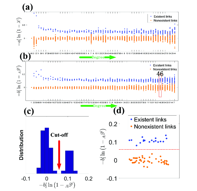
Figure 8: Reconstruction of CS-AARHUS duplex network. (a,b) Values of $-a_{l}^{i}\ln\left({1-{\lambda^{i}}}\right),~{}i\neq l$ and $-b_{l}^{i}\ln\left({1-{\lambda^{i}}}\right)~{}i\neq l$ (b) for each node, respectively. Each column gives the connectivity of a node. The blue and orange points denote the existent and nonexistent links, respectively. (c) Illustration of the choice of the threshold with node 46 [highlighted by the red dashed frame in (b)]. Shown is the distribution of the values of $-b_{l}^{46}\ln\left({1-{\lambda^{i}}}\right)$ for $l\neq 46$. The peak centered about zero corresponds to nonexistent links while the other peak corresponds to existent links. A threshold can be set within the gap between the two peaks. (d) The threshold is illustrated to distinguish the actual from the nonexistent links. The length of time series is $M$=30000. Other parameters are $\lambda=0.2$, ${}_{U}{\beta}=0.2$, ${}_{A}{\beta}=0.5{}_{U}{\beta}$, and $\mu=\delta=0.8$.

VII Reconstruction of duplex networks with heterogeneous rates of spreading dynamics

Figure 9 demonstrates that our framework can reconstruct duplex networks with heterogeneous rates of spreading dynamics. In particular, transmission rates $\lambda^{i}$ and ${}_{U}{\beta^{i}}$ are randomly chosen from the ranges (0.2, 0.4) and (0.3, 0.5), respectively. The recovery rates $\delta^{i}$ and $\mu^{i}$ are randomly picked up from the ranges (0.6, 1) and (0.6, 1), respectively. Note that ${}_{A}\beta^{i}=0.5{}_{U}\beta^{i}$.

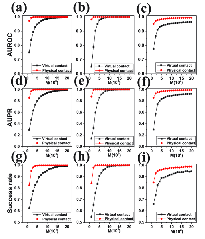
Figure 9: Applicability of reconstruction framework to spreading dynamics with heterogeneous rates. Reconstruction accuracy versus the length $M$ of the time series for ER-ER (left column), SW-SW (central column) and BA-BA (right column) duplex networks with heterogeneous transmission and recovery rates. The network parameters are $N=100$ and $\langle k_{1}\rangle=4,\langle k_{2}\rangle=6$.

References

- (1) Friston, K. J. Bayesian estimation of dynamical systems: an application to fMRI. NeuroImage 16, 513–530 (2002).
- (2) Gardner, T. S., di Bernardo, D., Lorenz, D. & Collins, J. J. Inferring genetic networks and identifying compound mode of action via expression profiling. Science 301, 102–105 (2003).
- (3) Pipa, G. & Grün, S. Non-parametric significance estimation of joint-spike events by shuffling and resampling. Neurocomp. 52, 31–37 (2003).
- (4) Brovelli, A. et al. Beta oscillations in a large-scale sensorimotor cortical network: directional influences revealed by Granger causality. Proc. Nat. Acad. Sci. (USA) 101, 9849–9854 (2004).
- (5) Eguiluz, V. M., Chialvo, D. R., Cecchi, G. A., Baliki, M. & Apkarian, A. V. Scale-free brain functional networks. Phys. Rev. Lett. 94, 018102 (2005).
- (6) Yu, D., Righero, M. & Kocarev, L. Estimating topology of networks. Phys. Rev. Lett. 97, 188701 (2006).
- (7) Bongard, J. & Lipson, H. Automated reverse engineering of nonlinear dynamical systems. Proc. Natl. Acad. Sci. (USA) 104, 9943–9948 (2007).
- (8) Timme, M. Revealing network connectivity from response dynamics. Phys. Rev. Lett. 98, 224101 (2007).
- (9) Napoletani, D. & Sauer, T. D. Reconstructing the topology of sparsely connected dynamical networks. Phys. Rev. E 77, 026103 (2008).
- (10) Donges, J., Zou, Y., Marwan, N. & Kurths, J. The backbone of the climate network. EPL (Europhys. Lett.) 87, 48007 (2009).
- (11) Pajevic, S. & Plenz, D. Efficient network reconstruction from dynamical cascades identifies small-world topology of neuronal avalanches. PLoS Comp. Biol. 5, e1000271 (2009).
- (12) Ren, J., Wang, W.-X., Li, B. & Lai, Y.-C. Noise bridges dynamical correlation and topology in coupled oscillator networks. Phys. Rev. Lett. 104, 058701 (2010).
- (13) Levnajić, Z. & Pikovsky, A. Network reconstruction from random phase resetting. Phys. Rev. Lett. 107, 034101 (2011).
- (14) Hempel, S., Koseska, A., Kurths, J. & Nikoloski, Z. Inner composition alignment for inferring directed networks from short time series. Phys. Rev. Lett. 107, 054101 (2011).
- (15) Shandilya, S. G. & Timme, M. Inferring network topology from complex dynamics. New J. Phys. 13, 013004 (2011).
- (16) Wang, W.-X., Lai, Y.-C., Grebogi, C. & Ye, J.-P. Network reconstruction based on evolutionary-game data via compressive sensing. Phys. Rev. X 1, 021021 (2011).
- (17) Berry, T., Hamilton, F., Peixoto, N. & Sauer, T. Detecting connectivity changes in neuronal networks. J. Neurosci. Meth. 209, 388–397 (2012).
- (18) Stetter, O., Battaglia, D., Soriano, J. & Geisel, T. Model-free reconstruction of excitatory neuronal connectivity from calcium imaging signals. PLoS Comp. Biol. 8, e1002653 (2012).
- (19) Su, R.-Q., Wang, W.-X. & Lai, Y.-C. Detecting hidden nodes in complex networks from time series. Phys. Rev. E 85, 065201 (2012).
- (20) Hamilton, F., Berry, T., Peixoto, N. & Sauer, T. Real-time tracking of neuronal network structure using data assimilation. Phys. Rev. E 88, 052715 (2013).
- (21) Zhou, D., Xiao, Y., Zhang, Y., Xu, Z. & Cai, D. Causal and structural connectivity of pulse-coupled nonlinear networks. Phys. Rev. Lett. 111, 054102 (2013).
- (22) Ching, E. S. C., Lai, P.-Y. & Leung, C. Y. Extracting connectivity from dynamics of networks with uniform bidirectional coupling. Phys. Rev. E 88, 042817 (2013).
- (23) Timme, M. & Casadiego, J. Revealing networks from dynamics: an introduction. J. Phys. A. Math. Theo. 47, 343001 (2014).
- (24) Su, R.-Q., Lai, Y.-C. & Wang, X. Identifying chaotic FitzHugh-Nagumo neurons using compressive sensing. Entropy 16, 3889–3902 (2014).
- (25) Shen, Z.-S., Wang, W.-X., Fan, Y., Di, Z. & Lai, Y.-C. Reconstructing propagation networks with natural diversity and identifying hidden sources. Nat. Commun. 5, 4323 (2014).
- (26) Ching, E. S. C., Lai, P.-Y. & Leung, C. Y. Reconstructing weighted networks from dynamics. Phys. Rev. E 91, 030801 (2015).
- (27) Wang, W.-X., Lai, Y.-C. & Grebogi, C. Data based identification and prediction of nonlinear and complex dynamical systems. Phys. Rep. 644, 1–76 (2016).
- (28) Casadiego, J., Nitzan, M., Hallerberg, S. & Timme, M. Model-free inference of direct network interactions from nonlinear collective dynamics. Nat. Commun. 8, 2192 (2017).
- (29) Li, X. & Li, X. Reconstruction of stochastic temporal networks through diffusive arrival times. Nat. Commun. 8, 15729 (2017).
- (30) Chen, Y.-Z. & Lai, Y.-C. Sparse dynamical Boltzmann machine for reconstructing complex networks with binary dynamics. Phys. Rev. E 97, 032317 (2018).
- (31) Mei, G. et al. Compressive-sensing-based structure identification for multilayer networks. IEEE Trans. Cybernet 48, 754–764 (2018).
- (32) Nitzan, M., Casadiego, J. & Timme, M. Revealing physical interaction networks from statistics of collective dynamics. Sci. Adv. 3 (2017).
- (33) Ma, C., Zhang, H.-F. & Lai, Y.-C. Reconstructing complex networks without time series. Phys. Rev. E 96, 022320 (2017).
- (34) Wang, W.-X., Yang, R., Lai, Y.-C., Kovanis, V. & Harrison, M. A. F. Time-series-based prediction of complex oscillator networks via compressive sensing. EPL (Europhys. Lett.) 94, 48006 (2011).
- (35) Buldyrev, S. V., Parshani, R., Paul, G., Stanley, H. E. & Havlin, S. Catastrophic cascade of failures in interdependent networks. Nature 464, 1025 (2010).
- (36) Gao, J., Buldyrev, S. V., Stanley, H. E. & Havlin, S. Networks formed from interdependent networks. Nat. Phys. 8, 40 (2012).
- (37) De Domenico, M. et al. Mathematical formulation of multilayer networks. Phys. Rev. X 3, 041022 (2013).
- (38) Kivelä, M. et al. Multilayer networks. J. Complex Net. 2, 203–271 (2014).
- (39) De Domenico, M., Granell, C., Porter, M. A. & Arenas, A. The physics of spreading processes in multilayer networks. Nat. Phys. 12, 901 (2016).
- (40) Granell, C., Gómez, S. & Arenas, A. Dynamical interplay between awareness and epidemic spreading in multiplex networks. Phys. Rev. Lett. 111, 128701 (2013).
- (41) Magnani, M., Micenkova, B. & Rossi, L. Combinatorial analysis of multiple networks. arXiv preprint arXiv:1303.4986 (2013).
- (42) Coleman, J., Katz, E. & Menzel, H. The diffusion of an innovation among physicians. Sociometry 20, 253–270 (1957).
- (43) Watts, D. J. & Strogatz, S. H. Collective dynamics of small-world networks. Nature 393, 440–442 (1998).
- (44) Erdos, P. & Rényi, A. On the evolution of random graphs. Publ. Math. Inst. Hung. Acad. Sci 5, 17–60 (1960).
- (45) Barabási, A.-L. & Albert, R. Emergence of scaling in random networks. Science 286, 509–512 (1999).
- (46) Li, J.-W., Shen, Z.-S., Wang, W.-X., Grebogi, C. & Lai, Y.-C. Universal data-based method for reconstructing complex networks with binary-state dynamics. Phys. Rev. E 95, 032303 (2017).