Deterministic Stretchy Regression

Abstract

An extension of the regularized least-squares in which the estimation parameters are stretchable is introduced and studied in this paper. The solution of this ridge regression with stretchable parameters is given in primal and dual spaces and in closed-form. Essentially, the proposed solution stretches the covariance computation by a power term, thereby compressing or amplifying the estimation parameters. To maintain the computation of power root terms within the real space, an input transformation is proposed. The results of an empirical evaluation in both synthetic and real-world data illustrate that the proposed method is effective for compressive learning with high-dimensional data.

1 Introduction

1.1 Background

In the past few decades, linear prediction models were seen to be among the most popular choices for data fitting and pattern recognition. They remain as part of the most important tools in various scientific applications today. Consider a set of $M$ training observations $(\boldsymbol{x}_{i},y_{i})$, $i=1,...,M$. The value $y_{i}\in\mbox{$\mathbb{R}$}$ is regarded as an output or response associated with the input features $\boldsymbol{x}_{i}\in\mbox{$\mathbb{R}$}^{d}$ of the system to be learned. Based on these observations, a generalized linear prediction model [1] can be written as

$$g(\boldsymbol{x}_{i},\boldsymbol{\alpha})=\alpha_{0}+\sum^{D-1}_{j=1}p_{j}(\boldsymbol{x}_{i})\alpha_{j}=\boldsymbol{p}_{i}^{T}\boldsymbol{\alpha},\ \ i=1,...,M,$$ (1)

where $\boldsymbol{p}_{i}:=[1,p_{1}(\boldsymbol{x}_{i}),...,p_{D-1}(\boldsymbol{x}_{i})]^{T}$ maps the original input features $\boldsymbol{x}_{i}\in\mbox{$\mathbb{R}$}^{d}$ onto the transformed features $\boldsymbol{p}_{i}\in\mbox{$\mathbb{R}$}^{D}$ with corresponding weight coefficient vector $\boldsymbol{\alpha}=[\alpha_{0},\alpha_{1},...,$ $\alpha_{D-1}]^{T}\in\mbox{$\mathbb{R}$}^{D}$. Expression (1) can be seen as an expansion in the basis $\{\boldsymbol{p}_{i}\}_{i=1}^{M}$. Popular choices for such basis are Gaussian [2], Sigmoid [3], Polynomial [4, 5] or Random Projection [6] functions. For the given set of $M$ data samples, the associated multiple column vectors $\boldsymbol{p}_{1},\cdots,\boldsymbol{p}_{M}$ can be stacked as ${\bf P}=[\boldsymbol{p}_{1},...,\boldsymbol{p}_{M}]^{T}$ and the above generalized linear prediction model can be compactly written as

$${\bf g}(\boldsymbol{x},\boldsymbol{\alpha})={\bf P}\boldsymbol{\alpha},$$ (2)

where ${\bf g}=[g(\boldsymbol{x}_{1},\boldsymbol{\alpha}),...,g(\boldsymbol{x}_{M},\boldsymbol{\alpha})]^{T}$ contains the corresponding output predictions of the given samples.

Based on the Gaussian random design model, one seeks to reconstruct the unknown weight coefficients ($\boldsymbol{\alpha}$) from a set of noisy measurements $y_{i}=g(\boldsymbol{x}_{i},\boldsymbol{\alpha})+e_{i}$, $i=1,...,M$. Frequently, the random noise $e_{i}$ is assumed to have independent and identically distributed random entries with mean 0 and variance $\sigma^{2}$. From the perspective of cost minimization, a Least Squares (LS) regression can be applied to minimize the discrepancy between the model output and the target. The LS regression is based on the magnitudes of $e_{i}=y_{i}-g(\boldsymbol{\alpha},\boldsymbol{x}_{i})$ in the Sum of Squared Errors (SSE) sense:

$$\textrm{SSE}(\boldsymbol{\alpha}) = {\frac{1}{2}\sum^{M}_{i=1}e_{i}^{2}}=\frac{1}{2}\|{\bf y}-{\bf P}\boldsymbol{\alpha}\|^{2}_{2},$$ (3)

where ${\bf y}=[y_{1},...,y_{M}]^{T}$ and $\|\cdot\|_{2}$ denotes the $\ell^{2}$-norm of a vector.

In order to deal with possible ill-conditioning when solving the minimum SSE problem, a popular and yet effective choice is to include an $\ell^{2}$-norm related penalty term (i.e., $\|\boldsymbol{\alpha}\|_{2}^{2}:=\sum_{j=0}^{D-1}\alpha_{j}^{2}=\boldsymbol{\alpha}^{T}\boldsymbol{\alpha}$) while minimizing the SSE [1, 7]:

$$\textrm{SSE}_{ridge}(\boldsymbol{\alpha})=\frac{1}{2}\|{\bf y}-{\bf P}\boldsymbol{\alpha}\|^{2}_{2}+\frac{\lambda}{2}\|\boldsymbol{\alpha}\|_{2}^{2}.$$ (4)

The closed-form solution of (4) is

$$\boldsymbol{\alpha}=({\bf P}^{T}{\bf P}+\lambda{\bf I})^{-1}{\bf P}^{T}{\bf y},$$ (5)

where the scalar $\lambda$ is called a regularization factor and ${\bf I}$ is an identity matrix matching the dimension of ${\bf P}^{T}{\bf P}$. In the literature, this is known as ridge regression [7, 8, 9].

By generalizing the penalty norm term to arbitrary power $p>0$, as

$$\|\boldsymbol{\alpha}\|_{p}:=\left(\sum^{D-1}_{j=0}|\alpha_{j}|^{p}\right)^{1/p},$$ (6)

the problem of minimizing

$$\textrm{SSE}_{bridge}(\boldsymbol{\alpha})=\sum^{M}_{i=1}\left(y_{i}-\boldsymbol{p}^{T}_{i}\boldsymbol{\alpha}\right)^{2}+\lambda\|\boldsymbol{\alpha}\|_{p}^{p}$$ (7)

is then called a bridge regression [10], where $0<p<2$ is of particular interest due to its compression capability. When $p=1$, the Least Absolute Shrinkage and Selection Operator (LASSO, [11, 12]) solves the $\ell^{1}$-norm penalized regression problem. Several extensions to such a regularization solution search can be found treating the penalty norm term in various forms (see e.g., [13, 14, 15]). A popular example is the Elastic-Net [14], which stretches between LASSO and ridge regression, adopting $\lambda_{1}\|\boldsymbol{\alpha}\|_{1}+\lambda_{2}\|\boldsymbol{\alpha}\|^{2}_{2}$ as the penalty term in its naive form.

Apart from the above regularization based methods, an alternative approach to deal with the singularity of covariance matrix ${\bf P}^{T}{\bf P}$ (inner product) for under-determined systems is to express it in its dual form as ${\bf P}{\bf P}^{T}$ (outer product) where a constrained optimization problem can be posed [16] to find $\boldsymbol{\alpha}$ which

$${\rm minimizes} \|\boldsymbol{\alpha}\|^{2}_{2}$$ (8)

$${\rm subject\ to\ } {\bf y}={\bf P}\boldsymbol{\alpha}.$$

Here, an analytical solution can be obtained based on the non-singularity of ${\bf P}{\bf P}^{T}$ in the following form

$$\boldsymbol{\alpha}={\bf P}^{T}({\bf P}{\bf P}^{T})^{-1}{\bf y},$$ (9)

where the outer product term replaces the inner product term of the regularization approach. This solution is known as the minimum-norm or least-norm solution [17], which applies particularly well to an under-determined system when $M<d+1$ or $M<D$. The constrained optimization problem in (8) can, again, be generalized to

$${\rm minimize} \|\boldsymbol{\alpha}\|^{p}_{p}$$ (10)

$${\rm subject\ to\ } {\bf y}={\bf P}\boldsymbol{\alpha}.$$

This leads to solving the corresponding unconstrained minimization problem given by

$$\min_{\boldsymbol{\alpha}}\|\boldsymbol{\alpha}\|^{p}_{p}+\boldsymbol{\beta}^{T}({\bf y}-{\bf P}\boldsymbol{\alpha}),$$ (11)

where different choices of $p$ result in different parametric stretching. Here, the elements in vector $\boldsymbol{\beta}$ are known as the Lagrange multipliers, where each element corresponds to a given data sample.

This framework is well adopted in compressed sensing research [18, 19, 20, 21], where minimization of the $\ell^{0}$-norm related objective is adopted for parameter subsets selection [22, 23] and minimization of the $\ell^{1}$-norm related objective is adopted for an optimally sparse solution [24]. Our work here involves solving an approximated norm metric under this approach.

1.2 Motivation and Contributions

Except for the case when $p=2$, existing solutions to minimize an objective function containing an $\ell^{p}$-norm term ($\|\boldsymbol{\alpha}\|_{p}$) or its powered form ($\|\boldsymbol{\alpha}\|^{p}_{p}$) require an iterative search to locate the minimizer. For example, LASSO minimizes an objective function with an $\ell^{1}$-norm penalty term which renders the formulation nonlinear. This results in a quadratic programming problem, where no analytical or closed-form expression is known (see [7], page 68-69). The same issue applies to Elastic-Net because it is transformed into a LASSO problem for solution search [14]. For bridge regression [10], the formulation is non-convex when $p<1$ and hence major focus was paid to the case when $p\geqslant 1$ (see e.g., [25]). Bearing in mind its application to compressed estimation, the range $0\leqslant p<2$ is of particular interest. The solution of the bridge regression problem cannot be expressed in closed from because of the absolute operator in the norm term. Hence the solutions are obtained using iterative numerical algorithms.

Different from existing approaches in the literature [26, 27, 28, 29, 30, 31], we make an attempt to seek a closed-form solution without the need of any iterative search. Following [32], where the absolute operator in (6) was omitted, we propose to approximate the absolute operator by a smooth function. This gives rise to an approximated $p$-norm which is differentiable. Optimization of the approximated $p$-norm subject to data fitting turns out to suggest a possible solution in closed-form. Based on the relationship between the primal parameter and the dual parameter of a restricted feasible solution set, an extended solution for the least-squares regression is proposed.

Although the idea of using a differentiable approximation to the $\ell^{1}$-norm penalty has been explored earlier in the literature, an iterative search on the nonlinear formulation remains inevitable. These differentiable approximations include the epsL1 function, the Huber function and the log-barrier function (see e.g., [33, 34]). The epsL1 function is defined as $epsL1(\alpha_{j},\epsilon)=\sqrt{\alpha_{j}^{2}+\epsilon}$ and the Huber function is defined as $Huber(\alpha_{j},\epsilon)=\left\{\begin{array}[]{cc}\alpha_{j}^{2}/2\epsilon&\textrm{if\ }|\alpha_{j}|<\epsilon\\ |\alpha_{j}|-\epsilon/2&\textrm{otherwise}\\ \end{array}\right.$, with gradient
$\nabla_{\alpha_{j}}Huber(\alpha_{j},\epsilon)=\left\{\begin{array}[]{cc}\alpha_{j}/\epsilon&\textrm{if\ }|\alpha_{j}|<\epsilon\\ \mbox{${\rm sgn}$}(\alpha_{j})&\textrm{otherwise}\\ \end{array}\right.$. The log-barrier function is defined as $\mu\log c(\boldsymbol{\alpha})$ where a popular candidate for $c(\boldsymbol{\alpha})$ is $\|\boldsymbol{\alpha}\|^{2}_{2}$.

In this work, the epsL1 function, which has recently been shown to be the most computationally efficient smooth approximation to the absolute function [35], is adopted to approximate the absolute operator in the $\ell^{p}$-norm function (6) where an analytical solution is attempted. Hence, our contributions include: (i) a novel closed-form solution for an extended version of the least squares ridge regression that considers the possibility of stretchy parameters, (ii) an input transformation to facilitate the computation of power roots, (iii) a variance analysis regarding the proposed estimator, and (iv) the provision of extensive empirical evidence to validate the feasibility and usefulness of the proposed method. In particular, our experiments illustrate that the stretching works well for problems with high-dimensional inputs where matrix ill-conditioning could be an issue in under-determined systems.

The remainder of the paper is organized as follows. In the next section, an approximation to the $\ell^{p}$-norm metric and several related lemmas are introduced. These lemmas are useful to derive the solution of the optimization problem. The proposed solutions are next presented within the same section in primal and dual forms. This is followed by introducing a standardization and transformation process to put the data in perspective. In Section 3, two representative synthetic data sets are evaluated to illustrate the stretching ability of the proposed method. In Section 4, the numerical experiments are extended to real-world data sets to observe the feasibility of the proposed solution on large dimensional problems. Concluding remarks are given in Section 5.

2 Proposed Stretchy Regression

2.1 $\ell^{p}$-norm Approximation

Consider a positive valued penalty term that is an approximation of the $\ell^{p}$-norm, in which the absolute value in (6) is replaced by a differentiable function $f$:

$$\mbox{$|\!\!\wr{\boldsymbol{\alpha}}\wr\!\!|_{k}$}:=\left(\sum^{D-1}_{j=0}f(\alpha_{j})^{k}\right)^{1/k}\negthinspace\negthinspace.$$ (12)

Here, the power term $k$ replaces $p$ in the $\ell^{p}$-norm to avoid confusion with the generalized linear model term $p(\cdot)$ in (1). A convenient choice for such an approximation, which can be efficiently computed, is $f(\alpha_{j})=\sqrt{\alpha_{j}^{2}+\epsilon}$, $\epsilon>0$ (see [35]) and Fig. 1). Note that $\lim_{\epsilon\rightarrow 0}f(\cdot)=|\cdot|$ for arbitrary $\epsilon>0$. For finite $\epsilon$ the function $|\!\!\wr{\boldsymbol{\alpha}}\wr\!\!|_{k}$ is not a norm because it does not have the absolute homogeneity property. We shall call $|\!\!\wr{\cdot}\wr\!\!|_{k}$ (12) a $k$-measure operator for convenience hereon.

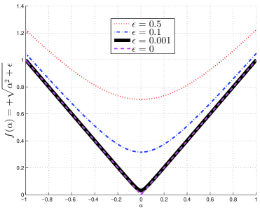
Figure 1: Plot of $f(\alpha)=\sqrt{\alpha^{2}+\epsilon}$ at several $\epsilon$ values.

In the following, the raised power form of $k$-measure is shown to be convex when the approximation function $f(\cdot)$ is convex.

Lemma 1

$|\!\!\wr{\boldsymbol{\alpha}}\wr\!\!|_{k}^{k}$ is convex on $\boldsymbol{\alpha}$ when $f$ is convex for all $k\geqslant 1$.

Proof: See Appendix A.

For our particular case of $f(\alpha_{i})=\sqrt{\alpha_{i}^{2}+\epsilon}$, it is easy to verify its convexity because the second derivative of $f(\alpha)$ for each $\alpha\in\{\alpha_{0},\alpha_{1},...,\alpha_{D-1}\}$ is

$$\frac{d^{2}f}{d\alpha^{2}}=\left(\alpha^{2}+\epsilon\right)^{-\frac{1}{2}}-\alpha^{2}\left(\alpha^{2}+\epsilon\right)^{-\frac{3}{2}},$$ (13)

where we see that

$$\frac{\left(\alpha^{2}+\epsilon\right)^{-\frac{1}{2}}}{\alpha^{2}\left(\alpha^{2}+\epsilon\right)^{-\frac{3}{2}}}=\frac{\alpha^{2}+\epsilon}{\alpha^{2}}>1,$$ (14)

for $\epsilon>0$, which implies convexity of $f$ on $\alpha$ based on $d^{2}f/d\alpha^{2}>0$.

Fig. 2 shows the contours of the $\ell^{p}$-norm metric (6) for $1<p<2$ and the corresponding ${k}$-measure ($|\!\!\wr{\boldsymbol{\alpha}}\wr\!\!|_{k}$, (12)) together with its $k$-powered form ($|\!\!\wr{\boldsymbol{\alpha}}\wr\!\!|_{k}^{k}$) within the same interval. From the bottom panels of Fig. 2, except for the difference in curvature, we see that the entire ${k}$-measure and its $k$-powered form approximate well to the solution $p$-norm for the plotted range of $1<\{p,k\}<2$. Particularly, for $p,k\rightarrow 1$, we shall show in Lemma 2 that the two solutions converge. This suggests vertices of the vector space being feasible solutions for the desired constrained solution search. Such observation shall be exploited in the following development for possible sparse solution when $1<k<2$.

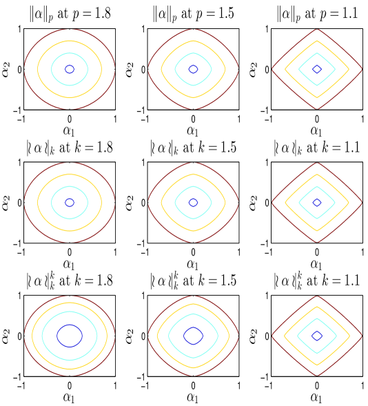
Figure 2: Contour plots at levels [0.1, 0.4, 0.7, 1]. Top panels: $\|\boldsymbol{\alpha}\|_{p}$ for $p\in\{1.8,1.5,1.1\}$. Middle Panels: $|\!\!\wr{\boldsymbol{\alpha}}\wr\!\!|_{k}$ for $k\in\{1.8,1.5,1.1\}$ at $\epsilon=0.0001$. Bottom Panels: $|\!\!\wr{\boldsymbol{\alpha}}\wr\!\!|_{k}^{k}$ for $k\in\{1.8,1.5,1.1\}$ at $\epsilon=0.0001$.

Lemma 2

$\lim_{q\rightarrow 1}\min_{\boldsymbol{\alpha}}\mbox{$|\!\!\wr{\boldsymbol{\alpha}}\wr\!\!|_{k}^{q}$}\ \,{\rm subject\ to\ \,}{\bf y}={\bf P}\boldsymbol{\alpha}$ is equivalent to $\min_{\boldsymbol{\alpha}}\mbox{$|\!\!\wr{\boldsymbol{\alpha}}\wr\!\!|_{k}$}\ \,{\rm subject\ to\ \,}{\bf y}={\bf P}\boldsymbol{\alpha}$, $\forall k\in\mbox{$\mathbb{R}$}$.

Proof: From (12), it is straightforward to check that $\mbox{$|\!\!\wr{\boldsymbol{\alpha}}\wr\!\!|_{k}$}=\mbox{$|\!\!\wr{\boldsymbol{\alpha}}\wr\!\!|_{k}$}^{q=1}=(\sum^{D-1}_{i=0}f(\alpha_{i})^{k})^{1/k}$ and $\lim_{q\rightarrow 1}\mbox{$|\!\!\wr{\boldsymbol{\alpha}}\wr\!\!|_{k}^{q}$}=\lim_{q\rightarrow 1}\left(\sum^{D-1}_{i=0}f(\alpha_{i})^{k}\right)^{q/k}=(\sum^{D-1}_{i=0}f(\alpha_{i})^{k})^{1/k}=\mbox{$|\!\!\wr{\boldsymbol{\alpha}}\wr\!\!|_{k}$}$. Hence the proof.  $\blacksquare$

When $q=k$, we have

Corollary 1

$\lim_{k\rightarrow 1}\min_{\boldsymbol{\alpha}}\mbox{$|\!\!\wr{\boldsymbol{\alpha}}\wr\!\!|_{k}^{k}$}\ \,{\rm subject\ to\ \,}{\bf y}={\bf P}\boldsymbol{\alpha}$ is equivalent to $\min_{\boldsymbol{\alpha}}\mbox{$|\!\!\wr{\boldsymbol{\alpha}}\wr\!\!|$}_{1}\ \,{\rm subject\ to\ \,}{\bf y}={\bf P}\boldsymbol{\alpha}$.

2.2 Stretchy Regression

With the above observations, we seek to minimize $|\!\!\wr{\boldsymbol{\alpha}}\wr\!\!|_{k}^{k}$ subject to ${\bf y}={\bf P}\boldsymbol{\alpha}$ as well as its regularized form by minimizing $\mbox{$|\!\!\wr{\boldsymbol{\alpha}}\wr\!\!|_{k}^{k}$}+\|\boldsymbol{e}\|^{2}_{2}$ subject to $\boldsymbol{e}={\bf y}-{\bf P}\boldsymbol{\alpha}$. Our goal is to have a sparse estimate in the limit of $k\rightarrow 1$. We will need the following Lemma 3 for our development of a deterministic solution. Denote the Hadamard product between vector $\boldsymbol{a}\in\mbox{$\mathbb{R}$}^{d}$ and vector $\boldsymbol{b}\in\mbox{$\mathbb{R}$}^{d}$ as $\boldsymbol{a}\circ\boldsymbol{b}$. By denoting the elementwise operation using $\circ{}$, we write the elementwise power of matrix/vector as ${\bf A}^{\mbox{\scriptsize$\circ{k}$}}$/${\bf b}^{\mbox{\scriptsize$\circ{k}$}}$ and the elementwise partial derivative of $\boldsymbol{a}$ with respect to $\boldsymbol{b}$ as $\frac{\partial\mbox{\scriptsize$\circ{\boldsymbol{a}}$}}{\partial\mbox{\scriptsize$\circ{\boldsymbol{b}}$}}$. For instance, ${\bf A}^{\mbox{\scriptsize$\circ{k}$}}:=[a_{ij}^{k}]$, for all $i,j$ which index the matrix elements. Then, consider a scaling vector which factors out ${\bf A}({\bf A}^{T}{\bf b})^{\mbox{\scriptsize$\circ{k}$}}$ as $({\bf A}({\bf A}^{T})^{\mbox{\scriptsize$\circ{k}$}}{\bf b}^{\mbox{\scriptsize$\circ{k}$}})\circ\boldsymbol{s}$ in the following lemma.

Lemma 3

Consider an $m\times d$ matrix ${\bf A}$ and a $m\times 1$ vector ${\bf b}$. Suppose $\sum^{d}_{j=1}a_{lj}\sum^{m}_{i=1}a_{ji}^{k}b_{i}^{k}\neq 0$ for all $l=1,...,m$, then there exists a scaling vector $\boldsymbol{s}$ such that ${\bf A}({\bf A}^{T}{\bf b})^{\mbox{\scriptsize$\circ{k}$}}=({\bf A}({\bf A}^{T})^{\mbox{\scriptsize$\circ{k}$}}{\bf b}^{\mbox{\scriptsize$\circ{k}$}})\circ\boldsymbol{s}$.

Proof: See Appendix B.

We are now ready to derive a deterministic solution for an approximated minimization problem to (11).

Theorem 1

Consider an under-determined system given by ${\bf y}={\bf P}\boldsymbol{\alpha}$ where ${\bf y}\in\mbox{$\mathbb{R}$}^{M}$, ${\bf P}\in\mbox{$\mathbb{R}$}^{M\times D}$ and $\boldsymbol{\alpha}\in\mbox{$\mathbb{R}$}^{D}$ with $M<D$. Suppose ${\bf P}({\bf P}^{T})^{\mbox{\scriptsize$\circ{\frac{1}{k-1}}$}}$ is of full rank, then for all $k>1$, $k\neq\infty$ and under the limiting case of ${\boldsymbol{\epsilon}\rightarrow{\bf 0}}$, the minimizer of

$$\min_{\boldsymbol{\alpha}}\mbox{$|\!\!\wr{\boldsymbol{\alpha}}\wr\!\!|_{k}^{k}$}\ \,{\rm subject\ to\ \,}{\bf y}={\bf P}\boldsymbol{\alpha},$$ (15)

satisfies

$${\bf P}\left(\boldsymbol{\alpha}-({\bf P}^{T})^{\mbox{\scriptsize$\circ{\frac{1}{k-1}}$}}\left({\bf P}({\bf P}^{T})^{\mbox{\scriptsize$\circ{\frac{1}{k-1}}$}}\right)^{-1}{\bf y}\right)={\bf 0}.$$ (16)

Proof: According to the definition of $k$-measure in (12), let $\bar{\boldsymbol{\alpha}}:=[(\alpha_{0}^{2}+\epsilon)^{{k}/4},\cdots,(\alpha_{D-1}^{2}+\epsilon)^{{k}/4}]^{T}$ where we can write $\mbox{$|\!\!\wr{\boldsymbol{\alpha}}\wr\!\!|_{k}$}=(\bar{\boldsymbol{\alpha}}^{T}\bar{\boldsymbol{\alpha}})^{1/k}$ and $\mbox{$|\!\!\wr{\boldsymbol{\alpha}}\wr\!\!|_{k}^{k}$}=(\bar{\boldsymbol{\alpha}}^{T}\bar{\boldsymbol{\alpha}})$. Then, taking the first derivative of the Lagrange function of (15) and setting it to zero gives:

$$\frac{\partial}{\partial\boldsymbol{\alpha}}\left(\bar{\boldsymbol{\alpha}}^{T}\bar{\boldsymbol{\alpha}}+\boldsymbol{\beta}^{T}({\bf y}-{\bf P}\boldsymbol{\alpha})\right) = {\bf 0}$$

$$\frac{k}{4}\cdot 2\boldsymbol{\alpha}\circ\left(\boldsymbol{\alpha}^{\mbox{\scriptsize$\circ{2}$}}+\boldsymbol{\epsilon}\right)^{\mbox{\scriptsize$\circ{\frac{k}{4}-1}$}}\circ 2\bar{\boldsymbol{\alpha}}-{\bf P}^{T}\boldsymbol{\beta} = {\bf 0}$$

$${k}\,\boldsymbol{\alpha}\circ\left(\boldsymbol{\alpha}^{\mbox{\scriptsize$\circ{2}$}}+\boldsymbol{\epsilon}\right)^{\mbox{\scriptsize$\circ{\frac{k}{4}-1}$}}\circ\left(\boldsymbol{\alpha}^{\mbox{\scriptsize$\circ{2}$}}+\boldsymbol{\epsilon}\right)^{\mbox{\scriptsize$\circ{\frac{k}{4}}$}}-{\bf P}^{T}\boldsymbol{\beta} = {\bf 0}$$

$$\Rightarrow\hskip 14.22636pt{k}\,\boldsymbol{\alpha}\circ\left(\boldsymbol{\alpha}^{\mbox{\scriptsize$\circ{2}$}}+\boldsymbol{\epsilon}\right)^{\mbox{\scriptsize$\circ{\frac{k}{2}-1}$}} = {\bf P}^{T}\boldsymbol{\beta}.\hskip 19.34787pt$$ (17)

For the limiting case of $\boldsymbol{\epsilon}$, we have

$$\lim_{\boldsymbol{\epsilon}\rightarrow{\bf 0}}{k}\,\boldsymbol{\alpha}\circ\left(\boldsymbol{\alpha}^{\mbox{\scriptsize$\circ{2}$}}+\boldsymbol{\epsilon}\right)^{\mbox{\scriptsize$\circ{\frac{k}{2}-1}$}} = {k}\,\boldsymbol{\alpha}\circ\left(\boldsymbol{\alpha}^{\mbox{\scriptsize$\circ{2}$}}\right)^{\mbox{\scriptsize$\circ{\frac{k}{2}-1}$}},$$ (18)

which implies that for all $k>1$ and $k\neq\infty$,

$${k}\,\boldsymbol{\alpha}\circ\left(\boldsymbol{\alpha}^{\mbox{\scriptsize$\circ{2}$}}\right)^{\mbox{\scriptsize$\circ{\frac{k-2}{2}}$}} = {\bf P}^{T}\boldsymbol{\beta}$$

$${k}\,\mbox{${\rm sgn}$}(\boldsymbol{\alpha})\circ(\boldsymbol{\alpha}^{\mbox{\scriptsize$\circ{2}$}})^{\frac{1}{2}}\circ\left(\boldsymbol{\alpha}^{\mbox{\scriptsize$\circ{2}$}}\right)^{\mbox{\scriptsize$\circ{\frac{k-2}{2}}$}} = {\bf P}^{T}\boldsymbol{\beta}$$

$${k}\,\mbox{${\rm sgn}$}(\boldsymbol{\alpha})\circ\left(\boldsymbol{\alpha}^{\mbox{\scriptsize$\circ{2}$}}\right)^{\mbox{\scriptsize$\circ{\frac{k-1}{2}}$}} = {\bf P}^{T}\boldsymbol{\beta}$$ (19)

$$\Rightarrow\hskip 14.22636pt\left(\boldsymbol{\alpha}^{\mbox{\scriptsize$\circ{2}$}}\right)^{\mbox{\scriptsize$\circ{\frac{k-1}{2}}$}}\ \ =\ \ \mbox{${\rm sgn}$}(\boldsymbol{\alpha})\circ\left(\frac{1}{k}{\bf P}^{T}\boldsymbol{\beta}\right).$$

Taking square elementwise for both sides of (19), we have

$$\left(\boldsymbol{\alpha}^{\mbox{\scriptsize$\circ{2}$}}\right)^{\mbox{\scriptsize$\circ{k-1}$}} = \left(\frac{1}{k}{\bf P}^{T}\boldsymbol{\beta}\right)^{\mbox{\scriptsize$\circ{2}$}}.$$ (20)

From (17), we know that the vector $\lim_{\boldsymbol{\epsilon}\rightarrow{\bf 0}}(\boldsymbol{\alpha}^{\mbox{\scriptsize$\circ{2}$}}+\boldsymbol{\epsilon})$ has positive elements and thus $\lim_{\boldsymbol{\epsilon}\rightarrow{\bf 0}}\left(\boldsymbol{\alpha}^{\mbox{\scriptsize$\circ{2}$}}+\boldsymbol{\epsilon}\right)^{\mbox{\scriptsize$\circ{\frac{k}{2}-1}$}}$ has positive elements regardless of $k$. Hence, we deduce that $\mbox{${\rm sgn}$}(\boldsymbol{\alpha})=\mbox{${\rm sgn}$}({\bf P}^{T}\boldsymbol{\beta})$, and

$$\boldsymbol{\alpha} = \left({\bf P}^{T}\left\{\frac{1}{k}\boldsymbol{\beta}\right\}\right)^{\mbox{\scriptsize$\circ{\frac{1}{k-1}}$}}.$$ (21)

For the matrix $({\bf P}^{T})^{\mbox{\scriptsize$\circ{\frac{1}{k-1}}$}}$ with elements $p_{ji}^{\frac{1}{k-1}}$, $j=0,...,{D-1}$, $i=1,...,M$ and the vector $\left\{\frac{1}{k}\boldsymbol{\beta}\right\}^{\mbox{\scriptsize$\circ{\frac{1}{k-1}}$}}$ with elements $\beta_{i}/k$, $i=1,...,M$, supposing $\sum^{D-1}_{i=0}p_{lj}\sum^{M}_{i=1}p_{ji}^{\frac{1}{k-1}}(\beta_{i}/k)^{\frac{1}{k-1}}\neq 0$ for all $l=1,...,M$, we can factor out (21) using Lemma 3, giving

$${\bf P}\boldsymbol{\alpha} = {\bf P}\left({\bf P}^{T}\left\{\frac{1}{k}\boldsymbol{\beta}\right\}\right)^{\mbox{\scriptsize$\circ{\frac{1}{k-1}}$}}$$ (22)

$$= \left({\bf P}({\bf P}^{T})^{\mbox{\scriptsize$\circ{\frac{1}{k-1}}$}}\left\{\frac{1}{k}\boldsymbol{\beta}\right\}^{\mbox{\scriptsize$\circ{\frac{1}{k-1}}$}}\right)\circ\boldsymbol{s}.$$

Next, replacing ${\bf P}\boldsymbol{\alpha}$ by ${\bf y}$ gives

$${\bf y} = \left({\bf P}({\bf P}^{T})^{\mbox{\scriptsize$\circ{\frac{1}{k-1}}$}}\left\{\frac{1}{k}\boldsymbol{\beta}\right\}^{\mbox{\scriptsize$\circ{\frac{1}{k-1}}$}}\right)\circ\boldsymbol{s}$$

$$\Rightarrow\hskip 8.53581pt\frac{1}{k}\boldsymbol{\beta} = \left[\left({\bf P}({\bf P}^{T})^{\mbox{\scriptsize$\circ{\frac{1}{k-1}}$}}\right)^{-1}{\bf y}\circ\boldsymbol{s}^{\mbox{\scriptsize$\circ{-1}$}}\right]^{\mbox{\scriptsize$\circ{k-1}$}}.$$ (23)

Substituting $\frac{1}{k}\boldsymbol{\beta}$ into (22) and simplifying, we have for all $k>1$, $k\neq\infty$ and the limiting case of $\boldsymbol{\epsilon}\rightarrow{\bf 0}$,

$${\bf P}\boldsymbol{\alpha} = \left({\bf P}({\bf P}^{T})^{\mbox{\scriptsize$\circ{\frac{1}{k-1}}$}}\left\{\frac{1}{k}\boldsymbol{\beta}\right\}^{\mbox{\scriptsize$\circ{\frac{1}{k-1}}$}}\right)\circ\boldsymbol{s}$$ (24)

$$= \left({\bf P}({\bf P}^{T})^{\mbox{\scriptsize$\circ{\frac{1}{k-1}}$}}\left({\bf P}({\bf P}^{T})^{\mbox{\scriptsize$\circ{\frac{1}{k-1}}$}}\right)^{-1}{\bf y}\circ\boldsymbol{s}^{\mbox{\scriptsize$\circ{-1}$}}\right)\circ\boldsymbol{s}$$

$$= {\bf P}({\bf P}^{T})^{\mbox{\scriptsize$\circ{\frac{1}{k-1}}$}}\left({\bf P}({\bf P}^{T})^{\mbox{\scriptsize$\circ{\frac{1}{k-1}}$}}\right)^{-1}{\bf y}.$$

As $\boldsymbol{s}$ vanishes in the above derivation, its possible singularity (i.e., even when $\sum^{D-1}_{j=0}p_{lj}$ $\sum^{M}_{i=1}p_{ji}^{\frac{1}{k-1}}(\beta_{i}/k)^{\frac{1}{k-1}}=0$, $l=1,...,M$) takes no effect in the resultant solution.

The above cannot be simplified further since ${\bf P}$ cannot be removed from the left in (24) due to its rank deficiency for $M<D$. Nevertheless, (24) implies (16) and gives the solution of $\boldsymbol{\alpha}$ implicitly, that is $(\boldsymbol{\alpha}-({\bf P}^{T})^{\mbox{\scriptsize$\circ{\frac{1}{k-1}}$}}({\bf P}({\bf P}^{T})^{\mbox{\scriptsize$\circ{\frac{1}{k-1}}$}})^{-1}{\bf y})$ lies in the null space of ${\bf P}$. The optimality of the minimizer comes from the summation of the convex $|\!\!\wr{\cdot}\wr\!\!|_{k}^{k}$ (Lemma 1) and linear $\boldsymbol{\beta}^{T}({\bf y}-{\bf P}\boldsymbol{\alpha})$ functions. Hence the result.  $\blacksquare$

A direct consequence of the above result is

Corollary 2

Suppose ${\bf P}({\bf P}^{T})^{\mbox{\scriptsize$\circ{\frac{1}{k-1}}$}}$ is of full rank. Then, by constraining the feasible solution space to $\boldsymbol{\alpha}=({\bf P}^{T})^{\mbox{\scriptsize$\circ{\frac{1}{k-1}}$}}\boldsymbol{\beta}$, $\forall\boldsymbol{\beta}\in\mbox{$\mathbb{R}$}^{M}$ for all $k>1$ and $k\neq\infty$, problem (15) admits the particular solution

$$\boldsymbol{\alpha}=\left({\bf P}^{T}\right)^{\mbox{\scriptsize$\circ{\frac{1}{k-1}}$}}\left[{\bf P}({\bf P}^{T})^{\mbox{\scriptsize$\circ{\frac{1}{k-1}}$}}\right]^{-1}{\bf y}.$$ (25)

Proof: The result is obtained by substituting $\boldsymbol{\alpha}=({\bf P}^{T})^{\mbox{\scriptsize$\circ{\frac{1}{k-1}}$}}\boldsymbol{\beta}$ into (24).  $\blacksquare$

Under practical considerations, an explicit suppression of the estimation noise along with the $k$-measure regularization is useful:

Theorem 2

Consider an under-determined system given by ${\bf y}={\bf P}\boldsymbol{\alpha}+\boldsymbol{e}$ where ${\bf y},\boldsymbol{e}\in\mbox{$\mathbb{R}$}^{M}$, ${\bf P}\in\mbox{$\mathbb{R}$}^{M\times D}$ and $\boldsymbol{\alpha}\in\mbox{$\mathbb{R}$}^{D}$ with $M<D$. Suppose ${\bf P}({\bf P}^{T})^{\mbox{\scriptsize$\circ{\frac{1}{k-1}}$}}$ is of full rank. Then, by restricting the feasible solution space to $\boldsymbol{\alpha}=({\bf P}^{T})^{\mbox{\scriptsize$\circ{\frac{1}{k-1}}$}}\boldsymbol{\beta}$ for all $k>1$ and $k\neq\infty$ on the Lagrange multipliers $\boldsymbol{\beta}\in\mbox{$\mathbb{R}$}^{M}$, minimization of

$$\mbox{$|\!\!\wr{\boldsymbol{\alpha}}\wr\!\!|_{k}^{k}$}+{c}\|\boldsymbol{e}\|^{2}_{2}$$ (26)

subject to the constraint

$$\boldsymbol{e}={\bf y}-{\bf P}\boldsymbol{\alpha}$$ (27)

under the limiting case of ${\boldsymbol{\epsilon}\rightarrow{\bf 0}}$ admits the solution

$$\boldsymbol{\alpha}=\left({\bf P}^{T}\right)^{\mbox{\scriptsize$\circ{\frac{1}{k-1}}$}}\left[{\bf P}({\bf P}^{T})^{\mbox{\scriptsize$\circ{\frac{1}{k-1}}$}}+\frac{1}{{c}k}{\bf I}\right]^{-1}{\bf y},$$ (28)

where $c>0$ is the regularization parameter.

Proof: Taking the first derivative of the Lagrange function and considering the independency of the random variable $\boldsymbol{e}$ under this dual space construction [36], we have

$$\frac{\partial}{\partial\boldsymbol{\alpha}}\left(\mbox{$|\!\!\wr{\boldsymbol{\alpha}}\wr\!\!|_{k}^{k}$}+{c}\boldsymbol{e}^{T}\boldsymbol{e}+\boldsymbol{\beta}^{T}({\bf y}-{\bf P}\boldsymbol{\alpha}-\boldsymbol{e})\right) = {\bf 0}$$

$$\Rightarrow\hskip 14.22636pt\frac{\partial}{\partial\boldsymbol{\alpha}}\left(\mbox{$|\!\!\wr{\boldsymbol{\alpha}}\wr\!\!|_{k}^{k}$}+\boldsymbol{\beta}^{T}({\bf y}-{\bf P}\boldsymbol{\alpha})\right) = {\bf 0}.$$ (29)

Similar to (17), solving (29) results in (19).

Substituting the error constraint (27) and the solution (19) into the cost function (26) under the limiting case of $\boldsymbol{\epsilon}\rightarrow{\bf 0}$ we have

$$\lim_{\boldsymbol{\epsilon}\rightarrow 0}\mbox{$|\!\!\wr{\boldsymbol{\alpha}}\wr\!\!|_{k}^{k}$}+{c}\boldsymbol{e}^{T}\boldsymbol{e} = ((\boldsymbol{\alpha}^{T})^{\mbox{\scriptsize$\circ{2}$}})^{\mbox{\scriptsize$\circ{\frac{k-1}{2}}$}}(\boldsymbol{\alpha}^{\mbox{\scriptsize$\circ{2}$}})^{\mbox{\scriptsize$\circ{\frac{1}{2}}$}}+{c}({\bf y}-{\bf P}\boldsymbol{\alpha})^{T}({\bf y}-{\bf P}\boldsymbol{\alpha})$$ (30)

$$= \left(\mbox{${\rm sgn}$}(\boldsymbol{\alpha}^{T})\circ\frac{1}{k}\boldsymbol{\beta}^{T}{\bf P}\right)\left(\boldsymbol{\alpha}\circ\mbox{${\rm sgn}$}(\boldsymbol{\alpha})\right)+{c}{\bf y}^{T}{\bf y}-2{c}{\bf y}^{T}{\bf P}\boldsymbol{\alpha}+{c}\boldsymbol{\alpha}^{T}{\bf P}^{T}{\bf P}\boldsymbol{\alpha}$$

$$= \frac{1}{k}\boldsymbol{\beta}^{T}{\bf P}\boldsymbol{\alpha}+{c}{\bf y}^{T}{\bf y}-2{c}{\bf y}^{T}{\bf P}\boldsymbol{\alpha}+{c}\boldsymbol{\alpha}^{T}{\bf P}^{T}{\bf P}\boldsymbol{\alpha}.$$

Since the solution is restricted to the subspace $\boldsymbol{\alpha}=({\bf P}^{T})^{\mbox{\scriptsize$\circ{\frac{1}{k-1}}$}}\boldsymbol{\beta}$, equation (30) can be written as

$$\lim_{\boldsymbol{\epsilon}\rightarrow 0}\mbox{$|\!\!\wr{\boldsymbol{\alpha}}\wr\!\!|_{k}^{k}$}+c\boldsymbol{e}^{T}\boldsymbol{e} = \frac{1}{k}\boldsymbol{\beta}^{T}{\bf P}({\bf P}^{T})^{\mbox{\scriptsize$\circ{\frac{1}{k-1}}$}}\boldsymbol{\beta}+{c}{\bf y}^{T}{\bf y}-2{c}{\bf y}^{T}{\bf P}({\bf P}^{T})^{\mbox{\scriptsize$\circ{\frac{1}{k-1}}$}}\boldsymbol{\beta}$$ (31)

$$\hskip 8.53581pt+{c}\boldsymbol{\beta}^{T}{\bf P}^{\mbox{\scriptsize$\circ{\frac{1}{k-1}}$}}{\bf P}^{T}{\bf P}({\bf P}^{T})^{\mbox{\scriptsize$\circ{\frac{1}{k-1}}$}}\boldsymbol{\beta}$$

$$= \frac{1}{k}\boldsymbol{\beta}^{T}{\bf K}\boldsymbol{\beta}+{c}{\bf y}^{T}{\bf y}-2{c}{\bf y}^{T}{\bf K}\boldsymbol{\beta}+{c}\boldsymbol{\beta}^{T}{\bf K}^{T}{\bf K}\boldsymbol{\beta},$$

where ${\bf K}={\bf P}({\bf P}^{T})^{\mbox{\scriptsize$\circ{\frac{1}{k-1}}$}}$.

Differentiating (31) with respect to $\boldsymbol{\beta}$ and put to zero gives

$$2\frac{1}{k}{\bf K}\boldsymbol{\beta}-2{c}{\bf K}{\bf y}+2{c}{\bf K}^{T}{\bf K}\boldsymbol{\beta} = {\bf 0}.$$ (32)

Since ${\bf K}$ is nonsingular, we have

$$(\frac{1}{k}{\bf K}+{c}{\bf K}^{T}{\bf K})\boldsymbol{\beta} = c{\bf K}{\bf y}$$

$$\Rightarrow\hskip 28.45274pt\boldsymbol{\beta} = {\bf K}^{-1}(\frac{1}{{c}k}{\bf I}+{\bf K})^{-1}{\bf K}{\bf y}.$$ (33)

Using the matrix identity $({\bf I}+{\bf A}{\bf B})^{-1}{\bf A}={\bf A}({\bf I}+{\bf B}{\bf A})^{-1}$ [37], the above can be simplified as

$$\boldsymbol{\beta} = {ck}{\bf K}^{-1}({\bf I}+{\bf K}{c}k)^{-1}{\bf K}{\bf y}$$ (34)

$$= {ck}{\bf K}^{-1}{\bf K}({\bf I}+{c}k{\bf K})^{-1}{\bf y}$$

$$= (\frac{1}{{c}k}{\bf I}+{\bf K})^{-1}{\bf y}.$$

The result (28) arises from substituting (34) into the restricted solution space $\boldsymbol{\alpha}=({\bf P}^{T})^{\mbox{\scriptsize$\circ{\frac{1}{k-1}}$}}\boldsymbol{\beta}$. Hence the proof.  $\blacksquare$

From minimizing the SSE perspective, the following result is a direct consequence.

Corollary 3

Suppose ${\bf P}({\bf P}^{T})^{\mbox{\scriptsize$\circ{\frac{1}{k-1}}$}}$ is of full rank. Then, by restricting the feasible solution space to $\boldsymbol{\alpha}=({\bf P}^{T})^{\mbox{\scriptsize$\circ{\frac{1}{k-1}}$}}\boldsymbol{\beta}$, $\forall\boldsymbol{\beta}\in\mbox{$\mathbb{R}$}^{M}$ and under the limiting case of $c\rightarrow\infty$, $\boldsymbol{\epsilon}\rightarrow{\bf 0}$, the problem (26)-(27) leads to SSE (3) which admits an extended least-squares solution in the form of (25) for all $k>1$ and $k\neq\infty$.

Proof: Substituting $\boldsymbol{\alpha}=({\bf P}^{T})^{\mbox{\scriptsize$\circ{\frac{1}{k-1}}$}}\boldsymbol{\beta}$ into the least-squares error objective function (3) and minimizing it with respect to $\boldsymbol{\beta}$, we have

$$\frac{\partial}{\partial\boldsymbol{\beta}}\left({\bf y}-{\bf P}({\bf P}^{T})^{\mbox{\scriptsize$\circ{\frac{1}{k-1}}$}}\boldsymbol{\beta}\right)^{T}\left({\bf y}-{\bf P}({\bf P}^{T})^{\mbox{\scriptsize$\circ{\frac{1}{k-1}}$}}\boldsymbol{\beta}\right)={\bf 0}$$

$$\Rightarrow\hskip 28.45274pt{\bf P}({\bf P}^{T})^{\mbox{\scriptsize$\circ{\frac{1}{k-1}}$}}\left({\bf y}-{\bf P}({\bf P}^{T})^{\mbox{\scriptsize$\circ{\frac{1}{k-1}}$}}\boldsymbol{\beta}\right)={\bf 0}$$

$$\Rightarrow\hskip 65.44142pt\boldsymbol{\beta}=\left[{\bf P}({\bf P}^{T})^{\mbox{\scriptsize$\circ{\frac{1}{k-1}}$}}\right]^{-1}{\bf y},$$ (35)

because ${\bf P}({\bf P}^{T})^{\mbox{\scriptsize$\circ{\frac{1}{k-1}}$}}$ is nonsingular. The solution (25) follows from substitution of (35) into $\boldsymbol{\alpha}=({\bf P}^{T})^{\mbox{\scriptsize$\circ{\frac{1}{k-1}}$}}\boldsymbol{\beta}$. Hence the result.  $\blacksquare$

Remark 1: When $c=0$, problem (26)-(27) becomes degenerate. This is because minimizing $|\!\!\wr{\boldsymbol{\alpha}}\wr\!\!|_{k}^{k}$ alone subject to the constraint $\boldsymbol{e}={\bf y}-{\bf P}\boldsymbol{\alpha}$ without specifying a bound is not meaningful.

When $c\rightarrow\infty$, problem (26)-(27) approaches problem (3), and the solution (28) approaches (25). Here, although the SSE objective function (3) does not involve any $k$ term, the particular solution (25), which contains the power term $1/(k-1)$, is one that arises from the restricted solution search space. In other words, given $M<D$, the restricted feasible space mapping $\boldsymbol{\alpha}=({\bf P}^{T})^{\mbox{\scriptsize$\circ{\frac{1}{k-1}}$}}\boldsymbol{\beta}$ projects the parameter vector $\boldsymbol{\alpha}\in\mbox{$\mathbb{R}$}^{D}$ onto a lower dimensional vector $\boldsymbol{\beta}\in\mbox{$\mathbb{R}$}^{M}$ for deterministic estimation of the under-determined system. When $k=2$, the solution (25) leads to (9). For $k<2$, we shall observe whether such stretchy estimation can be realized without impairing the estimation accuracy in the experiments. $\square$

Apart from the elementwise powered matrix, we further note that the solution forms (25) and (28) are analogous to that of the least-norm solution in (9) and its regularized form. Besides the parameter vector of interest ($\boldsymbol{\alpha}$), derivation of the above solution involves two other parameters $k$ and $c$. The parameter $k$ can be considered as a hyper-parameter to be pre-fixed for any desired compression level. This adds a degree of freedom for compressing the parameter vector of interest. The other hyper-parameter $c$ controls the amount of regularization. The impact of the values of $k$ and $c$ shall be studied in the analysis of variance and numerical experiments using both synthetic and real-world data.

2.3 Analysis of Variance

To analyze the performance of the estimator $\hat{\boldsymbol{\alpha}}$, we assume that ${\bf y}={\bf P}\boldsymbol{\alpha}+\boldsymbol{e}$ where $\boldsymbol{e}$ is an independent and identically distributed noise of zero mean with covariance matrix ${\bf C}$.

Let the size of $\boldsymbol{\alpha}$ be $D\times 1$ and that of ${\bf P}$ be $M\times D$. For under-determined systems (28), we have $M<D$. In such a case, the expectation of $\hat{\boldsymbol{\alpha}}$ is given by (see Appendix C):

$$E[\hat{\boldsymbol{\alpha}}] = \left({\bf P}^{T}\right)^{\mbox{\scriptsize$\circ{\frac{1}{k-1}}$}}\left[{\bf P}({\bf P}^{T})^{\mbox{\scriptsize$\circ{\frac{1}{k-1}}$}}+\frac{1}{{c}k}{\bf I}\right]^{-1}{\bf P}\boldsymbol{\alpha}.$$ (36)

In order for $E[\hat{\boldsymbol{\alpha}}]=\boldsymbol{\alpha}$, it is required that the matrix $\left({\bf P}^{T}\right)^{\mbox{\scriptsize$\circ{\frac{1}{k-1}}$}}\left[{\bf P}({\bf P}^{T})^{\mbox{\scriptsize$\circ{\frac{1}{k-1}}$}}+\frac{1}{{c}k}{\bf I}\right]^{-1}{\bf P}$ must be an $D\times D$ identity matrix, which is not possible since for $M<D$,
$\left({\bf P}^{T}\right)^{\mbox{\scriptsize$\circ{\frac{1}{k-1}}$}}\left[{\bf P}({\bf P}^{T})^{\mbox{\scriptsize$\circ{\frac{1}{k-1}}$}}+\frac{1}{{c}k}{\bf I}\right]^{-1}{\bf P}$ is at most of rank $M<D$. Hence, $\hat{\boldsymbol{\alpha}}$ is a biased estimator. This is similar to the LS estimator (with $k=2$). This result is congruence to the proposed compressed estimate where some parameters can vanish, causing $E[\hat{\boldsymbol{\alpha}}]\neq\boldsymbol{\alpha}$.

The corresponding covariance matrix of $\hat{\boldsymbol{\alpha}}$ is

$$E[(\hat{\boldsymbol{\alpha}}-E[\hat{\boldsymbol{\alpha}}])(\hat{\boldsymbol{\alpha}}-E[\hat{\boldsymbol{\alpha}}])^{T}] = \left\{\left({\bf P}^{T}\right)^{\mbox{\scriptsize$\circ{\frac{1}{k-1}}$}}\left[{\bf P}({\bf P}^{T})^{\mbox{\scriptsize$\circ{\frac{1}{k-1}}$}}+\frac{1}{{c}k}{\bf I}\right]^{-1}\right\}{\bf C}$$ (37)

$$\qquad\times\left\{\left({\bf P}^{T}\right)^{\mbox{\scriptsize$\circ{\frac{1}{k-1}}$}}\left[{\bf P}({\bf P}^{T})^{\mbox{\scriptsize$\circ{\frac{1}{k-1}}$}}+\frac{1}{{c}k}{\bf I}\right]^{-1}\right\}^{T}.$$

When $k=2$, it becomes the ordinary LS estimator and standard LS result can be applied to simplify the above expression.

Next, we proceed to convert the above solution in the dual space form (outer product form) to the primal form (inner product form). Based on the matrix identity ${\bf A}({\bf I}+{\bf B}{\bf A})^{-1}=({\bf I}+{\bf A}{\bf B})^{-1}{\bf A}$ [37], the solution (28) under the dual space can be re-written in the primal space after simple manipulations as

$$\boldsymbol{\alpha}=\left[({\bf P}^{T})^{\mbox{\scriptsize$\circ{\frac{1}{k-1}}$}}{\bf P}+\frac{1}{ck}{\bf I}\right]^{-1}\left({\bf P}^{T}\right)^{\mbox{\scriptsize$\circ{\frac{1}{k-1}}$}}{\bf y}.$$ (38)

For variance analysis, consider (38) with over-determined systems where $({\bf P}^{T})^{\mbox{\scriptsize$\circ{\frac{1}{k-1}}$}}{\bf P}$ is nonsingular. Let the size of $\boldsymbol{\alpha}$ be $D\times 1$ and that of ${\bf P}$ be $M\times D$. For even-determined and over-determined systems, we have $M\geqslant D$. In such a case, the expectation of $\hat{\boldsymbol{\alpha}}$ is given by

$$E[\hat{\boldsymbol{\alpha}}]=E\left[\left[({\bf P}^{T})^{\mbox{\scriptsize$\circ{\frac{1}{k-1}}$}}{\bf P}+\frac{1}{{c}k}{\bf I}\right]^{-1}\left({\bf P}^{T}\right)^{\mbox{\scriptsize$\circ{\frac{1}{k-1}}$}}({\bf P}\boldsymbol{\alpha})\right],$$ (39)

where $\lim_{c\rightarrow\infty}E[\hat{\boldsymbol{\alpha}}]=\boldsymbol{\alpha}.$ Hence, $\hat{\boldsymbol{\alpha}}$ is an un-biased estimator regardless of the value of $k$ and for a general ${\bf C}$ under the least-squares minimization case in (3) when $c\rightarrow\infty$. This may be considered as a generalization of the LS estimator (with $k=2$). Here, $\lim_{c\rightarrow\infty}E[\hat{\boldsymbol{\alpha}}]=\boldsymbol{\alpha}$ indicates that no parameter vanishes in the expectation. In other words, the analysis shows that estimation under the over-determined setting cannot be sparse for the proposed solution.

For this case with over-determined systems, the covariance matrix of $\hat{\boldsymbol{\alpha}}$ is

$$E[(\hat{\boldsymbol{\alpha}}-E[\hat{\boldsymbol{\alpha}}])(\hat{\boldsymbol{\alpha}}-E[\hat{\boldsymbol{\alpha}}])^{T}] = \left\{\left[({\bf P}^{T})^{\mbox{\scriptsize$\circ{\frac{1}{k-1}}$}}{\bf P}+\frac{1}{{c}k}{\bf I}\right]^{-1}\left({\bf P}^{T}\right)^{\mbox{\scriptsize$\circ{\frac{1}{k-1}}$}}\right\}{\bf C}$$ (40)

$$\qquad\times\left\{\left[({\bf P}^{T})^{\mbox{\scriptsize$\circ{\frac{1}{k-1}}$}}{\bf P}+\frac{1}{{c}k}{\bf I}\right]^{-1}\left({\bf P}^{T}\right)^{\mbox{\scriptsize$\circ{\frac{1}{k-1}}$}}\right\}^{T}.$$

Consider now some special cases. When $k=2$, it becomes the ordinary LS estimator and standard LS result can be applied to simplify the above (even for the general ${\bf C}$ matrix).

When $k\neq 2$, the situation becomes more complicated. Assume first that ${\bf C}=\sigma^{2}{\bf I}_{D}$. We have

$$E[(\hat{\boldsymbol{\alpha}}-E[\hat{\boldsymbol{\alpha}}])(\hat{\boldsymbol{\alpha}}-E[\hat{\boldsymbol{\alpha}}])^{T}] = \sigma^{2}\left\{\left[({\bf P}^{T})^{\mbox{\scriptsize$\circ{\frac{1}{k-1}}$}}{\bf P}+\frac{1}{{c}k}{\bf I}\right]^{-1}\left({\bf P}^{T}\right)^{\mbox{\scriptsize$\circ{\frac{1}{k-1}}$}}\left({\bf P}\right)^{\mbox{\scriptsize$\circ{\frac{1}{k-1}}$}}\right\}$$ (41)

$$\qquad\times\left\{\left[({\bf P}^{T})^{\mbox{\scriptsize$\circ{\frac{1}{k-1}}$}}{\bf P}+\frac{1}{{c}k}{\bf I}\right]^{-1}\right\}^{T}.$$

Since $k\neq 2$, $({\bf P}^{T})^{\mbox{\scriptsize$\circ{\frac{1}{k-1}}$}}{\bf P}\neq\left({\bf P}^{T}\right)^{\mbox{\scriptsize$\circ{\frac{1}{k-1}}$}}\left({\bf P}\right)^{\mbox{\scriptsize$\circ{\frac{1}{k-1}}$}}$. Hence,
$\left[({\bf P}^{T})^{\mbox{\scriptsize$\circ{\frac{1}{k-1}}$}}{\bf P}+\frac{1}{ck}{\bf I}\right]^{-1}\left({\bf P}^{T}\right)^{\mbox{\scriptsize$\circ{\frac{1}{k-1}}$}}\left({\bf P}\right)^{\mbox{\scriptsize$\circ{\frac{1}{k-1}}$}}\neq{\bf I}_{D}$. Therefore, unlike the case with $k=2$, the above expression cannot be simplified further in general.

Another issue is the singularity of the matrix $({\bf P}^{T})^{\mbox{\scriptsize$\circ{\frac{1}{k-1}}$}}{\bf P}$ or ${\bf P}({\bf P}^{T})^{\mbox{\scriptsize$\circ{\frac{1}{k-1}}$}}$. So far, we assume that it is invertible. For the case of $k=2$, the non-singularity of $({\bf P}^{T})^{\mbox{\scriptsize$\circ{\frac{1}{k-1}}$}}{\bf P}$ or ${\bf P}({\bf P}^{T})^{\mbox{\scriptsize$\circ{\frac{1}{k-1}}$}}$ is guaranteed by making ${\bf P}$ non-singular. However, this may no longer be true for $k\neq 2$. We limit our discussion to $1<k<\infty$ where $k$ can be a non-integer.

It is easy to show that when $k\rightarrow 1$, $\frac{1}{k-1}\rightarrow\infty$, and consequently, $({\bf P}^{T})^{\mbox{\scriptsize$\circ{\frac{1}{k-1}}$}}$ is approaching a rank 1 matrix even if ${\bf P}$ is non-singular. Similarly, it can be shown that when $k\rightarrow\infty$, $\frac{1}{k-1}\rightarrow 0$, and consequently, $({\bf P}^{T})^{\mbox{\scriptsize$\circ{\frac{1}{k-1}}$}}$ is approaching a rank 1 matrix even if ${\bf P}$ is non-singular. In both cases, $({\bf P}^{T})^{\mbox{\scriptsize$\circ{\frac{1}{k-1}}$}}{\bf P}$ and ${\bf P}({\bf P}^{T})^{\mbox{\scriptsize$\circ{\frac{1}{k-1}}$}}$ become rank 1 matrices also and it is hence non-invertible. We conjecture that $k=2$ is the most stable case (in terms of matrix regularity) and it tends to singular when $k$ is moving away from 2, in both directions.

In the experiments, we shall adopt (28) when dealing with under-determined systems and adopt (38) when dealing with over-determined systems.

2.4 First Quadrant Transformation

Consider a stacked set of raw training input data given by

$${\bf X}_{raw}=\stackrel{{\scriptstyle\left[\begin{array}[]{cccc}{\bf x}_{1}&{\bf x}_{2}&\cdots&{\bf x}_{d}\\ \end{array}\right]}}{{\overbrace{\left[\begin{array}[]{cccc}x_{11}&x_{12}&\cdots&x_{1d}\\ x_{21}&x_{22}&\cdots&x_{2d}\\ \vdots&\vdots&\ddots&\vdots\\ x_{M1}&x_{M2}&\cdots&x_{Md}\\ \end{array}\right]}}}=\left[\begin{array}[]{c}\boldsymbol{x}_{1}\\ \boldsymbol{x}_{2}\\ \vdots\\ \boldsymbol{x}_{M}\\ \end{array}\right].$$ (42)

A standardization is first performed for each data column by a $z$-score normalization based on the statistics of training set ($\mu_{{\bf x}_{j}}$ and $\sigma_{{\bf x}_{j}}$):

$$\underline{{\bf x}}_{j}=({\bf x}_{j}-\mu_{{\bf x}_{j}})/\sigma_{{\bf x}_{j}},\ j=1,...,d.$$ (43)

Then, an exponential function is adopted to map the standardized data into the first quadrant:

$$\breve{{\bf x}}=\exp(a\underline{{\bf x}}_{j}+\boldsymbol{b}_{j}).$$ (44)

Fig. 3 shows the plots of transforming the first two dimensions of the Madelon data by using $a=-0.2$ and $\boldsymbol{b}=\boldsymbol{0}$ of (44). Since the test data is assumed to be unseen, the $z$-score standardization for the test set has been performed based on the parameters (mean and variance) obtained from the training set. This results in a slight variation of data spread for each dimension. The proposed transformation mapping is seen to be nearly linear for the observed data range. The merit of such mapping is that it can be easily integrated as part of the feature transformation matrix ${\bf P}$ in (2).

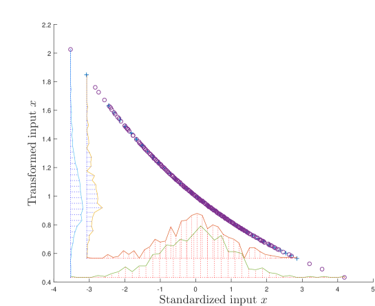
Figure 3: Transformation of the first two dimensions of the Madelon data. The shaded regions are the corresponding distributions of the input features.

Here, we note that the exponential transformation serves two purposes: first quadrant transformation and data warping. The main reason for the first quadrant transformation is to ensure that all input data contains only positive real values. This is to avoid occurrence of complex numbers when taking the fractional power of $1/(k-1)$ on negative elements of ${\bf P}$. The data warping mechanism twists the original data such that large values are far more distinguishable than those small values. This twisting further stretches (or compresses) the relative difference among the input variables on top of the stretchy regression.

3 Synthetic Data

In order to understand the stretching capability as well as the underlying decision boundary of the proposed method, two synthetic data examples are studied in this section. The first example demonstrates the scenario of an under-determined system for regression application. The second example represents an over-determined system for binary classification applications. We believe these two examples demonstrate several essential components of physical data distribution to help our study. The components of interest include nonlinearity, overlapping category distributions, under- and over-determined system scenarios.

Consider the first example, which contains five single-dimensional training samples (see the red circles in Fig. 4). These data points are generated using $y=1+0.6x-1.5x^{3}+0.8x^{4}$ based on $x\in\{0.1,0.2,0.3,0.4,0.5\}$. A polynomial model of $10^{th}$-order including the intercept term is adopted to fit these data points using the proposed stretchy regression. The solid lines in Fig. 4(a)-(b) shows the learned outputs at different $k$ and ${c}$ values. These results show good fitting when no noise is considered, i.e., the solid line passes through all data points marked by the red circles. Apart from the noiseless case, the learned outputs (marked by dashed lines) from ten ‘noisy’ measurements (marked by asterisks) are included in each figure. Here, due to the excessive number of parameters over the number of data samples, stretchy regression attempts to fit all the ‘noisy’ data points when ${c}$ is large (e.g., at negligible regularization such as ${c}=10^{15}$ in Fig. 4(a)). At $c=10^{4}$, the effect of regularization is observed to have a smoother fit where the noisy data points are not fully attempted in Fig. 4(b).

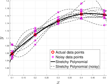
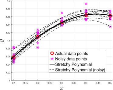
(a) ${k}=1.2$, ${c}=10^{15}$	(b) ${k}=1.8$, ${c}=10^{4}$

Figure 4: Learned outputs from noisy inputs at different ${k}$ and ${c}$ values.

Table 1 shows the variation of learned polynomial coefficients ($\hat{\boldsymbol{\alpha}}=[\hat{\alpha}_{0},...,\hat{\alpha}_{10}]^{T}$) at different ${k}$ and ${c}$ values. The results for both noiseless and noisy cases show convergence to a sparse solution when ${k}$ approaches $1$. Particularly, at $k=1.2$, the reconstructed polynomial coefficients for the noiseless case with weak regularization (at ${c}=10^{15}$, marked in boldface) compare relatively well with the ground truth ($\boldsymbol{\alpha}=[1,0.6,0,-1.5,0.8,0,\cdots,0]^{T}$). For stronger regularization at ${c}=10^{4}$, The estimation becomes smoother as evident from the low standard deviations. However, this comes at the price of having a lower fidelity to coefficient reconstruction. This is due to the heavier weight in regularization than error minimization.

Table 1: Average polynomial coefficient values estimated over 10 noiselsess/noisy samples at different ${k}$ and ${c}$ values

	${k}:1.8$, ${c}:10^{4}$	${k}:1.2$, ${c}:10^{4}$	${k}:1.8$, ${c}:10^{15}$	${k}:1.2$, ${c}:10^{15}$
	noiseless/noisy(std)	noiseless/noisy(std)	noiseless/noisy(std)	noiseless/noisy(std)
$\hat{\alpha}_{0}$	1.000/ 1.001( 0.019)	1.063/ 1.067( 0.014)	0.999/ 1.006( 0.186)	1.000/ 1.008( 0.237)
$\hat{\alpha}_{1}$	0.641/ 0.640( 0.142)	0.234/ 0.226( 0.045)	0.626/ 0.544( 3.033)	0.602/ 0.517( 4.181)
$\hat{\alpha}_{2}$	-0.402/-0.373( 0.380)	-0.046/-0.052( 0.018)	-0.198/ 0.118(14.957)	-0.014/ 0.331(24.060)
$\hat{\alpha}_{3}$	-0.340/-0.382( 0.171)	-0.002/-0.002( 0.001)	-0.826/-1.134(24.053)	-1.457/-1.854(55.477)
$\hat{\alpha}_{4}$	-0.179/-0.227( 0.250)	-0.000/-0.000( 0.000)	-0.140/-0.304( 1.298)	0.738/ 0.680(43.384)
$\hat{\alpha}_{5}$	-0.083/-0.114( 0.174)	-0.000/-0.000( 0.000)	0.219/ 0.210(12.138)	0.033/ 0.031( 1.944)
$\hat{\alpha}_{6}$	-0.036/-0.053( 0.097)	-0.000/-0.000( 0.000)	0.244/ 0.283(12.018)	0.001/ 0.001( 0.067)
$\hat{\alpha}_{7}$	-0.015/-0.024( 0.049)	-0.000/-0.000( 0.000)	0.168/ 0.204( 8.022)	0.000/ 0.000( 0.002)
$\hat{\alpha}_{8}$	-0.007/-0.011( 0.023)	-0.000/-0.000( 0.000)	0.095/ 0.118( 4.504)	0.000/ 0.000( 0.000)
$\hat{\alpha}_{9}$	-0.003/-0.005( 0.011)	-0.000/-0.000( 0.000)	0.049/ 0.061( 2.297)	0.000/ 0.000( 0.000)
$\hat{\alpha}_{10}$	-0.001/-0.002( 0.005)	-0.000/-0.000( 0.000)	0.024/ 0.030( 1.104)	0.000/ 0.000( 0.000)

In the second example, we consider the case of 20 two-dimensional data points with a few of them overlapping in class distribution. This constitutes an over-determined system when a 3rd-order bivariate polynomial model with 10 parameters is adopted. Fig. 5(a) shows the decision boundary plots of the polynomial model learned at $k=1.1$ and ${k}=2$ when ${c}=10^{100}$ (i.e., without regularization). Fig. 5(b) shows the estimated coefficients ($\hat{\boldsymbol{\alpha}}=[\hat{\alpha}_{0},...,\hat{\alpha}_{9}]$) at ${k}=1.1$. This result, however, does not show convergence to sparse solution when $k=1.1$. This is in congruence to our observation of the analysis of variance for over-determined systems.

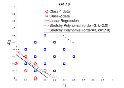
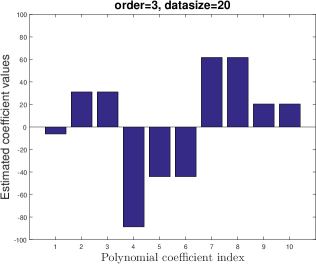
(a)	(b)

Figure 5: (a) Decision boundaries (at zero threshold level) of a linear model and a 3rd-order polynomial model learned from 20 data points at different ${k}$ values (all at ${c}=10^{100}$); (b) Estimated polynomial coefficient values at ${k}=1.1$.

Finally, the bivariate polynomial model is raised to 28th-order, where the total number of parameters to be estimated is 435. This turns the system an under-determined one since there are more parameters than data samples. Fig. 6(a) shows the decision contours for the polynomial model learned at $k=1.1$ and $k=2$ which are plotted together with the contour of the linear model. Here, the SR at $k=1.1$ gives 4 error count while the SR at $k=2$ gives 0 error count. Although the SR at $k=2$ produces no error, the decision contour becomes overly complex. This leads to an over-fitting scenario if the underlying distributions are not complex. Fig. 6(b) shows the sparseness of the estimated parameters at ${k}=1.1$. This example shows the applicability of SR in problems characterized by high-dimensional features with small number of samples.

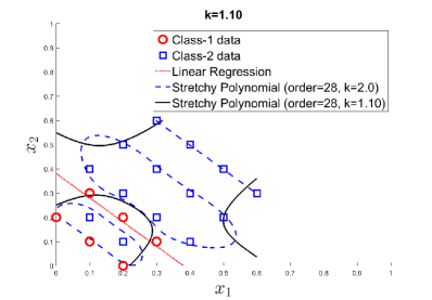
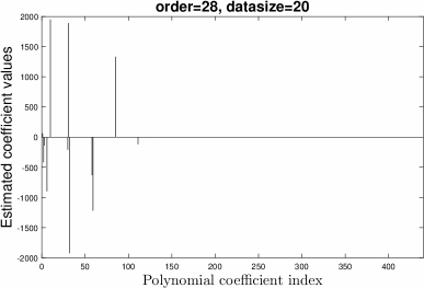
(a)	(b)

Figure 6: (a) Decision boundaries (at zero threshold level) of a linear model and a 28th-order polynomial model learned from 20 data points at different ${k}$ values (all at ${c}=10^{100}$); (b) Estimated polynomial coefficient values at ${k}=1.1$.

To summarize, the above synthetic examples illustrate stretching of relatively irrelevant weight coefficients towards zero for under-determined systems when $k\rightarrow 1$ while maintaining the necessary mapping. For over-determined systems, the stretching does not show sparseness when $k\rightarrow 1$. Apart from the much desired compressed estimation, the stretching capability offers beyond the fixed norm minimization which is particularly useful for numerical adaptation in practice. For example, when encountering numerical stability issue at $k=1.1$ for the given data set, a slightly higher value of $k$ (such as $k=1.2$) is yet available for a less compressed solution which comes with better numerical stability. In a nutshell, the stretching capability offers an adjustable mechanism for practicality. The effects of stretching on the estimation accuracy at various $k$ value settings are also observed in the following experiments on physical data.

4 Experiments on Physical Data

Apart from the regression problems, this study is extended to several binary classification problems to illustrate the applicability of the proposed method on physical data. Our first goal here is to observe whether the stretching can be applicable to physical data of high input dimensionality where matrix ill-conditioning is a commonly encountered problem. After verifying the applicability of parametric stretching, our subsequent goals are to observe whether the prediction accuracy can be impaired by the stretchy estimation and whether the training processing time is largely affected.

4.1 Data Sets

(i) Regression Data Sets

Five real-world regression problems from the public domain are utilized for this study. While the first two data sets represent over-determined systems, the remaining three data sets represent under-determined systems. The prostate cancer data set was adopted in [38], which came from a study in [39]. In this data set, the correlation between the level of prostate-specific antigen and several clinical measures was studied. The diabetes data set was adopted in [40], where ten baseline variables were obtained for each of 442 samples with a quantitative measure of disease progression one year after baseline. The corn data set consists of 80 samples of corn measured on three different NIR spectrometers with 700 channels [41, 42]. As a representative case in this study, we use m5spec to regress upon the moisture response.

E2006-TFIDF [43] is a text regression problem for predicting a real-world continuous quantity associated with the text’s meaning. In this study, the classic TFIDF (term-frequency/inverted-document-frequency) metric related to the frequency of occurrence of certain words within a document is adopted. The data set, which is of 150,360 dimensions, contains 3,308 samples for test and 16,087 samples for training. Due to our constraint in computing facilities, only the test set is utilized under a 2-fold cross-validation setting. Finally, we use the Columbia horizontal gaze data set for regression evaluation [44]. Each image has a resolution of 5,184 $\times$ 3,456 pixels. Again, due to the limitation of our computing facilities, only one-third (1960 samples) of the entire data (5880 samples) are utilized in this 2-fold evaluation. To further reduce the computational load, all the images are cropped to 1,200 $\times$ 1,000 pixels by removing much of the background. Each image is reshaped to a row vector of 1.2 million dimensions and stacked as a regressor matrix. Because the images contain only positive values normalized within [0,1], no further transformation is employed. A summary of these regression data sets is provided in Table 2.

Table 2: Regression data sets

Dataset	Domain	# Feat.	# Samples
Prostate	Medical	8	97
Diabetes	Medical	10	442
Corn	Spectrometry	700	80
TFIDF	Text	150,360	3,308
Gaze	Image	1,200,000	1,960

(ii) Binary Classification Data Sets

The classification problems of the NIPS feature selection challenge [45, 46] are utilized for this extended study. This challenge was introduced in 2003 with five high dimensional data sets, aiming to find feature selection algorithms that significantly outperform methods using all features. Each data set was partitioned into training, validation and test sets where the users were provided only the labels of training and validation sets together with their respective input features at the initial stage of challenge. Although the challenge ended in December 2003, the data sets are nevertheless available for evaluation and benchmarking of algorithms with only the test set labels withheld by the organizer. Table 3 provides an overview of the data sets in terms of the sizes of data and their feature dimension. Because the test data set is not available, we perform 10 trials of 2-fold cross-validation tests on all the available data, formed by combining the training set and the validation set.

Table 3: NIPS feature selection challenge data sets

Dataset	Domain	Type	# Feat.	# Trn	# Valid.	# Test
Arcene	Mass spec.	Dense	10000	100	100	700
Dexter	Text categ.	Sparse	20000	300	300	2000
Dorothea	Drug discov.	Sp. bin.	100000	800	350	800
Gisette	Digit recog.	Dense	5000	6000	1000	6500
Madelon	Artifical data	Dense	500	2000	600	1800

4.2 Evaluation Settings

To deal with inevitable statistical variations in experiments, we perform 10 trials of 2-fold tests on each data set. In terms of the accuracy measurement, the average mean squared error (MSE) of fitting is adopted for the regression data sets. For the classification data sets, the classification Balanced Error Rate (BER) is recorded in terms of its average values taken from these 10 trials of two-fold tests. For both the regression and the classification data sets, the average training CPU time in seconds (CPU) are recorded from the two-fold training process. The balanced error rate is defined as the average of the error rates of the positive class and the negative class. According to the provider of these data sets, this metric was used because some data sets are imbalanced. All experiments were conducted on a 64-bit Intel Core i7-3.6GHz processor with 16GB RAM, except for the TFIDF and Gaze data sets, which were evaluated on a 64-bit Intel Xeon E5-v2-3.5GHz processor with 64GB RAM.

Based on our empirical observation, a transformation using $a\in[-1,+1]$, $a\neq 0$ for most regression applications and at $a\in[-10,0)$ for most classification applications, all without inclusion of an offset ($\boldsymbol{b}={\bf 0}$, see (44)) produces reasonable results. Without diverting our focus towards data normalization issues, except for the Gaze data which used a normalized image with feature values falling within interval [0,1], all data sets are standardized for the proposed stretchy regression using a nominal setting of $a=-0.2$ and $\boldsymbol{b}={\bf 0}$ for positive quadrant transformation. For benchmarking purpose, the well-known LASSO [12] and Elastic-net [14] are included in the experiments alongside with the proposed stretchy regression. For convenience, we abbreviate the proposed stretchy regression as SR, and for LASSO-Elastic-net, the LASSO function [47] is adopted where it will be abbreviated as LASSO. This LASSO function traverses between LASSO ($\texttt{Alpha}=1$) and Elastic-net ($0<\texttt{Alpha}<1$) at various elastic net values (called Alpha, which controls the relative balance between $\ell^{1}$ and $\ell^{2}$ penalty) settings.

In order to gather a good picture regarding the sensitivity and performance over different algorithmic settings, the compared algorithms are evaluated under various parameter configurations. For the proposed algorithm, several stretching power values at ${k}\in\{1.1,1.25,1.5,1.75,2\}$ are experimented at regularization values ${c}\in\{10,10^{2},10^{3},10^{4},10^{8},10^{100}\}$ according to (28). We note that (25) is adopted for the case when ${c}=10^{100}$. For LASSO, the following elastic net mixing values are adopted: Alpha$\in\{1,0.75,0.5,0.25,0.0001\}$. Here we note that $\texttt{Alpha}=0$ is not allowed in the algorithm and it is equivalent to the ordinary $\ell^{2}$ regression and $k=2$ in our SR implementation. The elastic net mixing value Alpha in LASSO will be plotted alongside with $k$ values in SR in the experiments since they are related to elastic parametric solution even though not in exact sense due to their different optimization objectives.

Apart from Alpha, another setting for for LASSO is the sequence of lambda penalties which could affect the convergence of the solution. Here, the number of lambda values NumLambda is configured at 1, 2, 100 and a CV (cross-validated) search within the set $\{1,2,5,10,20,30,40,$ $60,80,100\}$ to observe its impact on the training CPU time and testing accuracy. Particularly, NumLambda=1 and NumLambda=CV explore the impact of having the lowest number of lambda penalties versus that selected from a large number of lambda penalties. We abbreviate these settings as LASSO1, LASSO2, LASSO100 and LASSOCV. For NumLambda$>1$, only the best accuracy in terms of lowest mean squared error is recorded.

Based on the above settings, both SR and LASSO are evaluated. Since the estimation by SR gives a smooth range of parametric values instead of a crisp set of sparse parameters, the proposed SR adopts a two-pass training process wherein the top parameter values from first-pass training are selected for a second-pass training according to user-specified feature density. For instance, for SR at 0.1 feature density, only the highest 10% of parameters, obtained from the first-pass training that utilizes all features, are selected for second-pass training. To observe the impact of sparse features for high dimensional data, we perform experiments on several feature density values, namely SR0.5, SR0.1 and SR0.01 together with the original SR1.0 with full features.

4.3 Results: Estimated Parameters

(i) Regression Problems: Fig. 7 shows some representative examples of the learned parameters for the proposed SR and the LASSO. These reported results had used (25) for learning in order to observe the extreme case without regularization. The parameters are sorted in ascending order for visualization purpose. For the Prostate (Fig. 7(a)-(b)) and the Diabetes (Fig. 7(c)-(d)) data sets, a sparse estimation for SR is not observed due to the over-determined problem nature. For the Corn (Fig. 7(e)-(f)), TFIDF (Fig. 7(g)-(h)) and Gaze (Fig. 7(i)-(j)) data sets, the estimated parameters are seen to have values with relatively large difference. Such difference in the estimated parameter values has been utilized for sparse parameter selection for the proposed SR. It is worth noting that for the TFIDF data set, a large proportion of the estimated parameter values are either zero or almost zero.

(ii) Classification Problems: Fig. 8 shows the exemplar estimated parameters which are sorted in ascending order for each of the classification data sets using (25). In most cases, the parameters are observed to have relatively large difference in terms of their estimation values. The sparse distribution of the parameters is particularly discernible for the Arcene, Dexter and Dorothea data sets (Fig. 8(a), (c), (e)). For the Gisette data set (Fig. 8(g) and (h)), the proposed SR show a relatively large difference in the magnitudes of parameters between $\alpha_{i}<0.5$ and $\alpha_{i}>0.5$, $i\in\{0,1,...,5000\}$. For the Madelon data set, Fig. 8(i) and (j) show a similar parameter distribution trend for both LASSO and SR except for their estimation value ranges. Due to the over-determined setting, the parameters do not show sparse distribution here.

4.4 Results: Prediction Accuracy

(A) Effect of ${k}$ values: In this part of the experiment, the impact of different ${k}$ values on the estimation accuracy is observed.

(i) Regression Problems: Fig. 9(a),(c),(e),(g),(i) show the accuracy results in terms of MSE for the SR and the LASSO on the regression data sets. Due to the relatively similar results at different regularization settings, only the results at ${c}=10^{2}$ are shown in these figures to avoid cluttering of plots, apart from the result for the non-regularized case using (25) (denoted as SR1.0(25)). For the Prostate and Diabetes data sets as shown in Fig. 9(a) and (c), a comparable MSE result is observed for both the SR and the LASSO except at LASSO1 setting. For the Corn data set in Fig. 9(e), the square root of MSE is adopted to reduce the many leading zeros of the MSE representation. These results show comparable performance between SR and LASSO. The MSE results for the TFIDF data set in Fig. 9(g) show a different behavior comparing with that of the Corn data set for the SR where the error bars show large standard deviations for most $k$ values. In contrast, LASSO shows a relatively stable MSE at all Alpha settings. Finally, the MSE results in terms of radian gaze angle in Fig. 9(i) show comparable performance of SR with that of LASSO only at large $k$-values ($k\geqslant 1.5$).

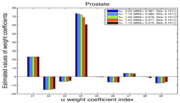
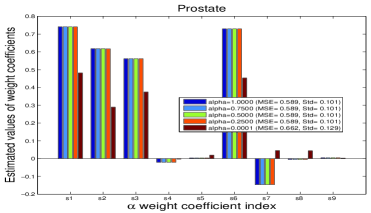
Prostate: (a) SR	(b) LASSO
$k\in\{1.1,1.25,1.5,1.75,2\}$	Alpha$\in\{1,0.75,0.5,0.25,0.0001\}$
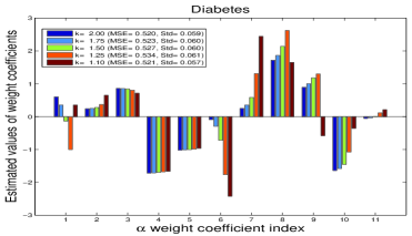
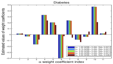
Diabetes: (c) SR	(d) LASSO
$k\in\{1.1,1.25,1.5,1.75,2\}$	Alpha$\in\{1,0.75,0.5,0.25,0.0001\}$
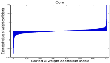
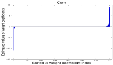
Corn: (e) SR at $k=1.1$	(f) LASSO at Alpha=1
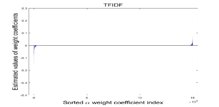
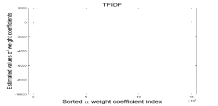
TFIDF: (g) SR at $k=1.25$	(h) LASSO at Alpha=1
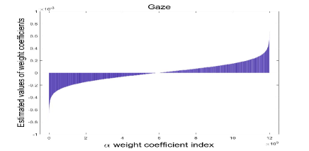
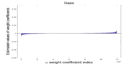
Gaze: (i) SR at $k=1.25$	(j) LASSO at Alpha=1

Figure 7: Regression: sorted parameter $\boldsymbol{\alpha}$ estimation values for the proposed SR and the LASSO.

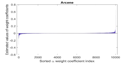
Arcene: (a) SR	(b) LASSO
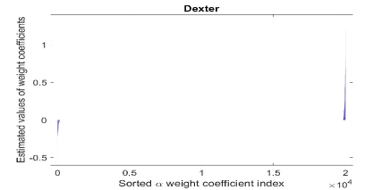
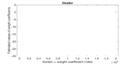
Dexter: (c) SR	(d) LASSO
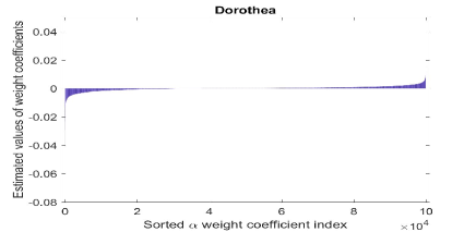
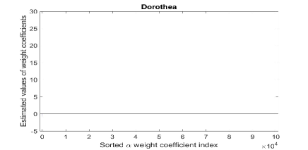
Dorothea: (e) SR	(f) LASSO
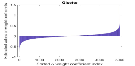
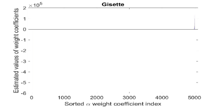
Gisette: (g) SR	(h) LASSO
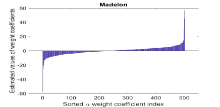
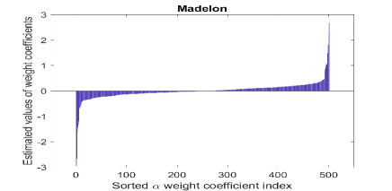
Madelon: (i) SR	(j) LASSO

Figure 8: Classification: sorted parameter $\boldsymbol{\alpha}$ estimation values for proposed SR at $k=1.1$ and LASSO at $\texttt{Alpha}=1$.

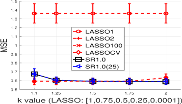
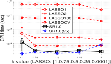
Prostate: (a) MSE	(b) CPU
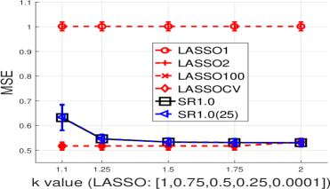
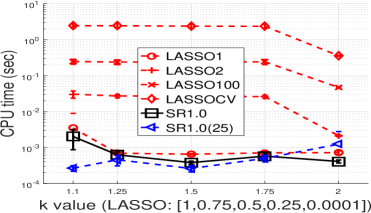
Diabetes: (c) MSE	(d) CPU
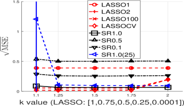
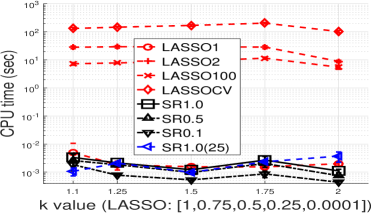
Corn: (e) $\sqrt{\rm MSE}$	(f) CPU
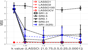
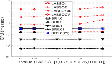
TFIDF: (g) MSE	(h) CPU
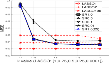
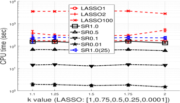
Gaze: (i) MSE	(j) CPU

Figure 9: Regression: MSE and CPU plots for SR at $k\in\{1.1,1.25,1.5,1.75,2\}$ and LASSO at Alpha$\in\{1,0.75,0.5,0.25,0.0001\}$.

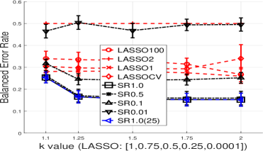
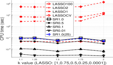
Arcene: (a) BER	(b) CPU
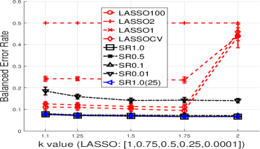
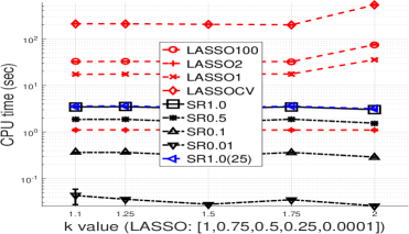
Dexter: (c) BER	(d) CPU
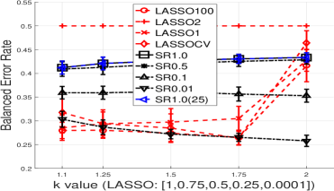
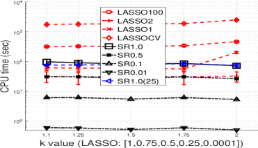
Dorothea: (e) BER	(f) CPU
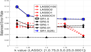
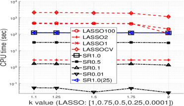
Gisette: (g) BER	(h) CPU
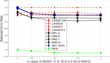
Madelon: (i) BER	(j) CPU

Figure 10: Classification: BER and CPU plots for SR at $k\in\{1.1,1.25,1.5,1.75,2\}$ and LASSO at Alpha$\in\{1,0.75,0.5,0.25,0.0001\}$. The CPU for RPN is plotted over projection sizes 500, 1000, 5000, 10000 and 20000.

(ii) Classification Problems: Fig. 10(a),(c),(e),(g),(i) show the accuracy results in terms of BER for the SR and the LASSO on the NIPS data sets, at ${c}=10^{2}$ and one using (25) for similar reasons. The classification accuracy for the Arcene data set in terms of BER is shown in Fig. 10(a) where the proposed SR is evaluated at various $k$ values ($k\in\{1.1,1.25,1.5,1.75,2\}$) at different sparseness levels namely, SR1.0, SR0.5, SR0.1 and SR0.01. The results of LASSO for various Alpha values (elastic net mixing value) at four NumLambda settings (LASSO1, LASSO2, LASSO100 and LASSOCV) are plotted in the same figure for comparison. In terms of BER, the proposed SR outperforms LASSO at various feature densities (SR1.0, SR0.5 and SR0.1) except for SR0.01. The prediction accuracy results for Dexter is shown in Fig. 10(c) where the BER trend is apparently similar to that of the Arcene example with the lowest performance goes to SR0.01 and the higher performances go to SR1.0, SR0.5 and SR0.1. This shows at least 10% of the parameters are useful for estimation in SR learning for this case. Different from the first two examples, in the Dorothea example of Fig. 10(e), the highly sparse SR (SR0.01) gives the best BER performance compared with that of LASSO. For the Gisette data set in Fig. 10(g), SR0.1 achieves the best performance while SR1.0 exhibits the worst performance among the compared classifiers. Fig. 10(i) show the BER performance for SR and LASSO at various settings on the Madelon data set. Here, although some of the SR settings show better BER performance compared to LASSO, the results are far from satisfactory (only around 45% BER) due to noninformative features. To validate the need of a nonlinear decision hyperplane on relevant features, an additional experiment is carried out on correlated features selected according to the dot product between the input vector and the target vector. An empirically selected eight features are then projected to high dimensions (500, 1000, 5000, 10000 and 20000) using a random projection network (RPN) [6]. The results show a significant improvement of BER for over 20%. This verifies the need of correlated features with nonlinear mapping capability beyond the evaluated linear SR and LASSO for this data set.

(B) Effect of ${c}$ values: Next, we observe the impact of regularization settings by varying the ${c}$ values in $\{10,10^{2},10^{3},10^{4},10^{100}\}$ at ${k}=1.25$. Fig. 11 shows the plots of prediction accuracies for both the regression and the binary classification problems. These results show that the estimations are relatively insensitive to the variation of ${c}$ except for the TFIDF data set where a significantly large variation of the error rate is observed at ${c}=10^{100}$.

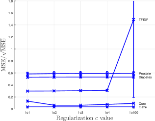
(a) Regression data	(b) Classification data

Figure 11: Error rates versus regularization ${c}$ values at ${k}=1.25$ and SR1.0: (a) MSE/$\sqrt{\rm MSE}$, (b) BER.

4.5 Processing Time

(i) Regression Problems: Fig. 9(b),(d),(f),(h),(j) show the average training CPU times in seconds for the SR and the LASSO on respective regression data sets. For the Prostate data set, Fig. 9(b) shows that SR is up to three thousand times faster than LASSO in terms of training time. For the Diabetes data set, Fig. 9(d) shows that SR is up to nine thousand times faster than LASSO. For the Corn data set, Fig. 9(f) shows no significant difference between SR1.0 and LASSO1 in execution time. However, the execution time of LASSO2, LASSO100 and LASSOCV slows down significantly due to inclusion of a penalty search in their implementation. For the TFIDF data set, Fig. 9(h) shows that the execution time of SR1.0 is observed to be nearly twice slower than that of LASSO1. However, when a penalty search is involved, the speed of LASSO slows down significantly. Finally, for the Gaze data set, LASSO100 shows significantly longer search times compared with all other algorithmic settings as seen from Fig. 9(j). LASSOCV was not included in this experiment due to its excessively long search time. In summary, we see that LASSO depends much on the NumLambda values search process whereas the proposed SR depends on the selected training feature dimension.

(ii) Classification Problems: Fig. 10(b),(d),(f),(h),(j) show the average training CPU times in seconds for the SR and the LASSO on respective classification data sets. For the Arcene data set, Fig. 10(b) shows a comparable speed between SR and LASSO1. However, when the NumLambda values are set beyond 1, the search process in LASSO significantly slows down its training speed. The training CPU time in Fig. 10(d) for the Dexter data set shows a trend similar to that of the Arcene example. For the Dorothea data set, the training CPU time as seen from Fig. 10(f) for SR is comparable with that of LASSO except for LASSO100 and LASSOCV which have the largest training CPU times. This is due to the large operating matrix dimension of this data set. For the Gisette data set, the training CPU times for all SR settings and LASSO1 in Fig. 10(h) are seen to be significantly lower than those of LASSOCV, LASSO100 and LASSO2. Fig. 10(j) shows the processing times for the Madelon data set. The increasing trend of processing time for the RPN is due to the increasing re-projected network sizes.

4.6 Summary of Results and Discussion

The experiments on regression problems show comparable MSE performance between SR and LASSO. In terms of execution time, SR is on par with LASSO without penalty search. However, when penalty search is included in LASSO (i.e., when NumLambda$>1$), the efficiency of SR becomes obvious.

For the extension of regression to binary classification problems, because a complete set of experiments for each algorithmic setting is available, we are able to perform a Friedman test to see whether the comparisons in Fig. 10 are significantly different in statistical sense. The confidence levels obtained for each comparison metric are respectively, BER with $p=0.0595$ and CPU with $p=4.2142\times 10^{-6}$. This suggests that we cannot reject the null hypothesis that all compared algorithms have similar performance in terms of BER where the observed differences are merely random at $95\%$ confidence level. However, from the Nemenyi test [48] plots as shown in Fig. 12(a) and (b), we observe a significant difference between the training CPU time of LASSO and SR when penalty search is involved in LASSO (such as that in LASSOCV, LASSO100 and LASSO2). Here, consistent with the Friedman test, the BER performance of penalty search based LASSOs do not differ significantly from those of SR. Without inclusion of penalty search, LASSO1 shows significantly lower BER performance than SR.

In summary, these experiments show the applicability of the proposed SR to real-world problems. Particularly the ${k}$ values are found to produce good accuracy at ${k}\geqslant 1.25$ and ${k}\geqslant 1.1$ respectively for regression and classification problems. It is noted that the closer is the ${k}$ value to one, the higher is the compression. However, due to the numerical stability of the term $1/(k-1)$ when $k\rightarrow 1$, the accuracy can be affected. Hence, in practice, the ${k}$ value can be chosen based on the lowest possible value near one with an accuracy performance comparable with that when ${k}=2$. The observed impact of regularization on the estimation error rate is not significant when ${c}$ is chosen within the range $[10,10^{4}]$. While an in-depth study of noise tolerance would be a valuable topic for future work, we observe here a significantly faster training time of SR over that of LASSO with a penalty search. Under relatively simple settings, the proposed SR shows predictive accuracy comparable with that of LASSO for both regression (in terms of MSE) and binary classification (in terms of BER) problems.

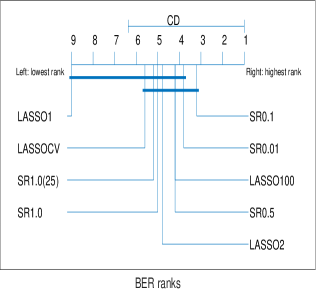
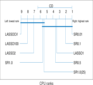
(a) Nemenyi test for BER results	(b) Nemenyi test for CPU results.

Figure 12: Nemenyi tests for binary classification problems.

5 Conclusion

In this paper, a stretchy regression was proposed for learning of linear parametric models beyond existing means. Essentially, a closed-form solution with feature warping capability was derived in primal and dual forms, analogous to that of ridge regression. Because the solution was operated upon positive and real input values, an exponential transformation was proposed to convert the inputs to the positive real axes. Under the space responsible for compressed estimation, it turned out that the solution enabled a seamless combination of feature extraction and learning within a single framework. Our experiments validated the feasibility of such regression for both synthetic and physical data learning.

Appendix A Proof of Lemma 1 on convexity of $k$-measure

Proof: Based on the convexity of $f$ on each element $\alpha_{i}$, $i=0,1,...,D-1$ (of the parameter vector $\boldsymbol{\alpha}$), we have

$$f(\lambda\alpha_{i1}+(1-\lambda)\alpha_{i2})\leqslant\lambda f(\alpha_{i1})+(1-\lambda)f(\alpha_{i2}),\ \ \ 0\leqslant\lambda\leqslant 1.$$ (45)

Suppose $h(\theta):=\theta^{k}$ with $k,\theta>0$ where we know that $h$ is nondecreasing and convex on $\theta$ since $dh/d\theta=k\theta^{k-1}\geqslant 0$ and $d^{2}h/d\theta^{2}=k(k-1)\theta^{k-2}\geqslant 0$, $\forall k\geqslant 1$ (see also [49]). Using (45) plus the fact that $h$ is nondecreasing and convex, we have for each $i=0,1,...,D-1$,

$$h(f(\lambda\alpha_{i1}+(1-\lambda)\alpha_{i2})) \leqslant h(\lambda f(\alpha_{i1})+(1-\lambda)f(\alpha_{i2}))$$ (46)

$$\leqslant \lambda h(f(\alpha_{i1}))+(1-\lambda)h(f(\alpha_{i2})),\ \ \ 0\leqslant\lambda\leqslant 1.$$

Since summation of convex functions preserves the convexity, we have

$$\sum^{D-1}_{i=0}h(f(\lambda\alpha_{i1}+(1-\lambda)\alpha_{i2}))\leqslant\sum^{D-1}_{i=0}\lambda h(f(\alpha_{i1}))+(1-\lambda)h(f(\alpha_{i2})),\ \ 0\leqslant\lambda\leqslant 1,$$ (47)

which means convexity of $\sum^{D-1}_{i=0}h(\alpha_{i})=\sum^{D-1}_{i=0}f(\alpha_{i})^{k}=\mbox{$|\!\!\wr{\boldsymbol{\alpha}}\wr\!\!|_{k}^{k}$}$ on $\boldsymbol{\alpha}=[\alpha_{0},\alpha_{1},...,\alpha_{D-1}]^{T}$. Hence the proof.  $\blacksquare$

Appendix B Proof of Lemma 3 on power of matrix-vector product factorization

Proof: By direct multiplication, we have

$${\bf A}(({\bf A}^{T}){\bf b})^{\mbox{\scriptsize$\circ{k}$}}=$$ (60)

$$\left[\begin{array}[]{cccc}a_{11}&a_{12}&\cdots&a_{1d}\\ a_{21}&a_{22}&\cdots&a_{2d}\\ \vdots&\vdots&\ddots&\vdots\\ a_{m1}&a_{m2}&\cdots&a_{md}\\ \end{array}\right]\left(\left[\begin{array}[]{cccc}a_{11}&a_{21}&\cdots&a_{m1}\\ a_{12}&a_{22}&\cdots&a_{m2}\\ \vdots&\vdots&\ddots&\vdots\\ a_{1d}&a_{2d}&\cdots&a_{md}\\ \end{array}\right]\left[\begin{array}[]{c}b_{1}\\ b_{2}\\ \vdots\\ b_{m}\\ \end{array}\right]\right)^{\mbox{\scriptsize$\circ{k}$}}$$

$$= \left[\begin{array}[]{cccc}a_{11}&a_{12}&\cdots&a_{1d}\\ a_{21}&a_{22}&\cdots&a_{2d}\\ \vdots&\vdots&\ddots&\vdots\\ a_{m1}&a_{m2}&\cdots&a_{md}\\ \end{array}\right]\left[\begin{array}[]{c}(\sum^{m}_{i=1}a_{1i}b_{i})^{k}\\ (\sum^{m}_{i=1}a_{2i}b_{i})^{k}\\ \vdots\\ (\sum^{m}_{i=1}a_{di}b_{i})^{k}\\ \end{array}\right]$$ (69)

$$= \left[\begin{array}[]{c}\sum^{d}_{j=1}a_{1j}(\sum^{m}_{i=1}a_{ji}b_{i})^{k}\\ \sum^{d}_{j=1}a_{2j}(\sum^{m}_{i=1}a_{ji}b_{i})^{k}\\ \vdots\\ \sum^{d}_{j=1}a_{mj}(\sum^{m}_{i=1}a_{ji}b_{i})^{k}\\ \end{array}\right]$$ (74)

$$= \left[\begin{array}[]{c}\sum^{d}_{j=1}a_{1j}\sum^{m}_{i=1}a_{ji}^{k}b_{i}^{k}\\ \sum^{d}_{j=1}a_{2j}\sum^{m}_{i=1}a_{ji}^{k}b_{i}^{k}\\ \vdots\\ \sum^{d}_{j=1}a_{mj}\sum^{m}_{i=1}a_{ji}^{k}b_{i}^{k}\\ \end{array}\right]\circ\left[\begin{array}[]{c}\frac{\sum^{d}_{j=1}a_{1j}(\sum^{m}_{i=1}a_{ji}b_{i})^{k}}{\sum^{d}_{j=1}a_{1j}\sum^{m}_{i=1}a_{ji}^{k}b_{i}^{k}}\\ \frac{\sum^{d}_{j=1}a_{2j}(\sum^{m}_{i=1}a_{ji}b_{i})^{k}}{\sum^{d}_{j=1}a_{2j}\sum^{m}_{i=1}a_{ji}^{k}b_{i}^{k}}\\ \vdots\\ \frac{\sum^{d}_{j=1}a_{mj}(\sum^{m}_{i=1}a_{ji}b_{i})^{k}}{\sum^{d}_{j=1}a_{mj}\sum^{m}_{i=1}a_{ji}^{k}b_{i}^{k}}\\ \end{array}\right]$$

$$= ({\bf A}(({\bf A}^{T})^{\mbox{\scriptsize$\circ{k}$}}{\bf b}^{\mbox{\scriptsize$\circ{k}$}}))\circ\boldsymbol{s}$$

$$= ({\bf A}({\bf A}^{T})^{\mbox{\scriptsize$\circ{k}$}}{\bf b}^{\mbox{\scriptsize$\circ{k}$}})\circ\boldsymbol{s},\textrm{by\ associative\ law\ }$$ (84)

for all $\sum^{d}_{j=1}a_{lj}\sum^{m}_{i=1}a_{ji}^{k}b_{i}^{k}\neq 0$, $l=1,...,m$. Hence the result.  $\blacksquare$

Appendix C Derivations for Analysis of Variance

The analysis is based on ${\bf y}={\bf P}\boldsymbol{\alpha}+\boldsymbol{e}$ where $\boldsymbol{e}$ is an independently and identically distributed noise of zero mean with covariance matrix ${\bf C}$.

For the under-determined system, the expectation of $\hat{\boldsymbol{\alpha}}$ based on (28) is given by

$$E[\hat{\boldsymbol{\alpha}}] = E\left[\left({\bf P}^{T}\right)^{\mbox{\scriptsize$\circ{\frac{1}{k-1}}$}}\left[{\bf P}({\bf P}^{T})^{\mbox{\scriptsize$\circ{\frac{1}{k-1}}$}}+\frac{1}{{c}k}{\bf I}\right]^{-1}({\bf P}\boldsymbol{\alpha}+\boldsymbol{e})\right]$$

$$= E\left[\left({\bf P}^{T}\right)^{\mbox{\scriptsize$\circ{\frac{1}{k-1}}$}}\left[{\bf P}({\bf P}^{T})^{\mbox{\scriptsize$\circ{\frac{1}{k-1}}$}}+\frac{1}{{c}k}{\bf I}\right]^{-1}({\bf P}\boldsymbol{\alpha})\right],$$

$$= \left({\bf P}^{T}\right)^{\mbox{\scriptsize$\circ{\frac{1}{k-1}}$}}\left[{\bf P}({\bf P}^{T})^{\mbox{\scriptsize$\circ{\frac{1}{k-1}}$}}+\frac{1}{{c}k}{\bf I}\right]^{-1}{\bf P}\boldsymbol{\alpha}.$$

which is equal to (36). The corresponding covariance matrix of $\hat{\boldsymbol{\alpha}}$ is derived as

$$E[(\hat{\boldsymbol{\alpha}}-E[\hat{\boldsymbol{\alpha}}])(\hat{\boldsymbol{\alpha}}-E[\hat{\boldsymbol{\alpha}}])^{T}] = E\left[\left\{\left({\bf P}^{T}\right)^{\mbox{\scriptsize$\circ{\frac{1}{k-1}}$}}\left[{\bf P}({\bf P}^{T})^{\mbox{\scriptsize$\circ{\frac{1}{k-1}}$}}+\frac{1}{{c}k}{\bf I}\right]^{-1}\boldsymbol{e}\right\}\right.$$

$$\qquad\times\left.\left\{\left({\bf P}^{T}\right)^{\mbox{\scriptsize$\circ{\frac{1}{k-1}}$}}\left[{\bf P}({\bf P}^{T})^{\mbox{\scriptsize$\circ{\frac{1}{k-1}}$}}+\frac{1}{{c}k}{\bf I}\right]^{-1}\boldsymbol{e}\right\}^{T}\right]$$

$$= \left\{\left({\bf P}^{T}\right)^{\mbox{\scriptsize$\circ{\frac{1}{k-1}}$}}\left[{\bf P}({\bf P}^{T})^{\mbox{\scriptsize$\circ{\frac{1}{k-1}}$}}+\frac{1}{{c}k}{\bf I}\right]^{-1}\right\}{\bf C}$$

$$\qquad\qquad\times\left\{\left({\bf P}^{T}\right)^{\mbox{\scriptsize$\circ{\frac{1}{k-1}}$}}\left[{\bf P}({\bf P}^{T})^{\mbox{\scriptsize$\circ{\frac{1}{k-1}}$}}+\frac{1}{{c}k}{\bf I}\right]^{-1}\right\}^{T}.$$

which gives rise to (37).

For the over-determined system, the expectation of $\hat{\boldsymbol{\alpha}}$ is given by (39) based on the following derivation:

$$E[\hat{\boldsymbol{\alpha}}] = E\left[\left[({\bf P}^{T})^{\mbox{\scriptsize$\circ{\frac{1}{k-1}}$}}{\bf P}+\frac{1}{{c}k}{\bf I}\right]^{-1}\left({\bf P}^{T}\right)^{\mbox{\scriptsize$\circ{\frac{1}{k-1}}$}}({\bf P}\boldsymbol{\alpha}+\boldsymbol{e})\right]$$

$$= E\left[\left[({\bf P}^{T})^{\mbox{\scriptsize$\circ{\frac{1}{k-1}}$}}{\bf P}+\frac{1}{{c}k}{\bf I}\right]^{-1}\left({\bf P}^{T}\right)^{\mbox{\scriptsize$\circ{\frac{1}{k-1}}$}}({\bf P}\boldsymbol{\alpha})\right].$$

The corresponding covariance matrix of $\hat{\boldsymbol{\alpha}}$ is

$$E[(\hat{\boldsymbol{\alpha}}-E[\hat{\boldsymbol{\alpha}}])(\hat{\boldsymbol{\alpha}}-E[\hat{\boldsymbol{\alpha}}])^{T}] = E\left[\left\{\left[({\bf P}^{T})^{\mbox{\scriptsize$\circ{\frac{1}{k-1}}$}}{\bf P}+\frac{1}{{c}k}{\bf I}\right]^{-1}\left({\bf P}^{T}\right)^{\mbox{\scriptsize$\circ{\frac{1}{k-1}}$}}\boldsymbol{e}\right\}\right.$$

$$\qquad\times\left.\left\{\left[({\bf P}^{T})^{\mbox{\scriptsize$\circ{\frac{1}{k-1}}$}}{\bf P}+\frac{1}{{c}k}{\bf I}\right]^{-1}\left({\bf P}^{T}\right)^{\mbox{\scriptsize$\circ{\frac{1}{k-1}}$}}\boldsymbol{e}\right\}^{T}\right]$$

$$= \left\{\left[({\bf P}^{T})^{\mbox{\scriptsize$\circ{\frac{1}{k-1}}$}}{\bf P}+\frac{1}{ck}{\bf I}\right]^{-1}\left({\bf P}^{T}\right)^{\mbox{\scriptsize$\circ{\frac{1}{k-1}}$}}\right\}{\bf C}$$

$$\qquad\qquad\times\left\{\left[({\bf P}^{T})^{\mbox{\scriptsize$\circ{\frac{1}{k-1}}$}}{\bf P}+\frac{1}{ck}{\bf I}\right]^{-1}\left({\bf P}^{T}\right)^{\mbox{\scriptsize$\circ{\frac{1}{k-1}}$}}\right\}^{T}.$$

which gives rise to (40).

References

- [1] R. O. Duda, P. E. Hart, and D. G. Stork, Pattern Classification, 2nd ed. New York: John Wiley & Sons, Inc, 2001.
- [2] T. Poggio and F. Girosi, “Networks for approximation and learning,” Proceedings of the IEEE, vol. 78, no. 9, pp. 1481–1497, 1990.
- [3] C. M. Bishop, Neural Networks for Pattern Recognition. New York: Oxford University Press Inc., 1995.
- [4] W. Campbell, K. Torkkola, and S. Balakrishnan, “Dimension reduction techniques for training polynomial networks,” in International Conference on Machine Learning (ICML), Stanford, CA, USA, June 2000.
- [5] K.-A. Toh, Q.-L. Tran, and D. Srinivasan, “Benchmarking a reduced multivariate polynomial pattern classifier,” IEEE Trans. on Pattern Analysis and Machine Intelligence, vol. 26, no. 6, pp. 740–755, 2004.
- [6] K.-A. Toh, “Deterministic neural classification,” Neural Computation, vol. 20, no. 6, pp. 1565–1595, June 2008.
- [7] T. Hastie, R. Tibshirani, and J. Friedman, The Elements of Statistical Learning: Data Mining, Inference, and Prediction. Canada: Springer, 2001.
- [8] A. N. Tikhonov, “Solution of incorrectly formulated problems and the regularization method,” Doklady Akademii Nauk SSSR, vol. 151, pp. 501 –504, 1963, translated in Soviet Mathematics 4: 1035-1038.
- [9] A. E. Hoerl and R. W. Kennard, “Ridge regression: Biased estimation for nonorthogonal problems,” Technometrics, vol. 12, pp. 55–67, 1970.
- [10] I. E. Frank and J. H. Friedman, “A statistical view of some chemometrics regression tools,” Technometrics, vol. 35, pp. 109–148, 1993.
- [11] R. Tibshirani, “Regression shrinkage and selection via the lasso: a retrospective,” J. Roy. Statist. Soc. Ser. B, vol. 73, pp. 273–282, 2011, part 3.
- [12] ——, “Regression shrinkage and selection via the lasso,” J. Roy. Statist. Soc. Ser. B, vol. 58, pp. 267–288, 1996.
- [13] R. Mazumder and T. Hastie, “The graphical lasso: New insights and alternatives,” Electronic Journal of Statistics, vol. 6, pp. 2125 –2149, 2012.
- [14] H. Zou and T. Hastie, “Regularization and variable selection via the elastic net,” Journal of the Royal Statistical Society, Series B, vol. 67, pp. 301–320, 2005, (Part 2).
- [15] M. Yuan and Y. Lin, “Model selection and estimation in regression with grouped variables,” Journal of the Royal Statistical Society, Series B, vol. 68, pp. 49–67, 2006, (Part 1).
- [16] W. R. Madych, “Solutions of underdetermined systems of linear equations,” in Lecture Notes – Monograph Series, Spatial Statistics and Imaging, 1991, vol. 20, pp. 227–238, institute of Mathematical Statistics.
- [17] S. Boyd and L. Vandenberghe, Convex Optimization. Cambridge: Cambridge University Press, 2004.
- [18] D. L. Donoho, “Compressed sensing,” IEEE Trans. on Information Theory, vol. 52, no. 4, pp. 1289 –1306, 2006.
- [19] R. G. Baraniuk, “Compressive sensing,” IEEE Signal Processing Magazine, vol. 24, no. 4, pp. 118– 124, July 2007.
- [20] E. J. Candés and M. B. Wakin, “An introduction to compressive sampling,” IEEE Signal Processing Magazine, vol. 52, no. 2, pp. 21 –30, March 2008.
- [21] M. E. Ahsen, N. Challapalli, and M. Vidyasagar, “Two new approaches to compressed sensing exhibiting both robust sparse recovery and the grouping effect,” Journal of Machine Learning Research, vol. 18, pp. 1–24, 2017.
- [22] A. Miller, Subset Selection in Regression. London: CHAPMAN & HALL/CRC (A CRC Press Company), 2002.
- [23] E. L. Dyer, A. C. Sankaranarayanan, and R. G. Baraniuk, “Greedy feature selection for subspace clustering,” Journal of Machine Learning Research, vol. 14, pp. 2487–2517, 2013.
- [24] D. L. Donoho and M. Elad, “Optimally sparse representation in general (nonorthogonal) dictionaries via minimization,” Proceedings of the National Academy of Sciences of the United States of America, vol. 100, no. 5, pp. 2197– 2202, 2003.
- [25] W. J. Fu, “Penalized regressions: The bridge versus the lasso,” Journal of Computational and Graphical Statistics, vol. 7, no. 3, pp. 397 –416, 1998.
- [26] D. L. Donoho, Y. Tsaig, I. Drori, and J.-L. Starck, “Sparse solution of underdetermined linear equations by stagewise orthogonal matching pursuit,” IEEE Trans. on Information Theory, vol. 58, no. 2, pp. 1094– 1121, 2012.
- [27] J. H. Friedman, “Fast sparse regression and classification,” International Journal of Forecasting, vol. 28, no. 3, pp. 722– 738, 2012.
- [28] T. T. Cai and L. Wang, “Orthogonal matching pursuit for sparse signal recovery with noise,” IEEE Trans. on Information Theory, vol. 57, no. 7, pp. 4680 –4688, 2011.
- [29] M. A. Figueiredo, “Adaptive sparseness for supervised learning,” IEEE Transactions on Pattern Analysis and Machine Intelligence, vol. 25, no. 9, pp. 1150–1159, September 2003.
- [30] P. B. Nair, A. Choudhury, and A. J. Keane, “Some greedy learning algorithms for sparse regression and classification with mercer kernels,” Journal of Machine Learning Research, vol. 3, pp. 781–801, 2002.
- [31] P. Pokarowski and J. Mielniczuk, “Combined and greedy penalized least squares,” Journal of Machine Learning Research, vol. 16, pp. 961–992, 2015.
- [32] K.-A. Toh, “Twisting key absolute space for stretchy polynomial regression,” in Proceedings of the 13th International Conference on Automation, Robotics and Computer Vision (ICARCV), Singapore, December 2014, pp. 953–957.
- [33] S.-I. Lee, H. Lee, P. Abbeel, and A. Y. Ng, “Efficient L1 regularized logistic regression,” in Proceedings of The Twenty-First National Conference on Artificial Intelligence and the Eighteenth Innovative Applications of Artificial Intelligence Conference (AAAI), Boston, Massachusetts, USA, July 2006, pp. 401–408.
- [34] M. Schmidt, “Graphical model structure learning with L1-regularization,” Ph.D. dissertation, University of British Columbia, 2010.
- [35] C. Ramirez, R. Sanchez, V. Kreinovich, and M. Argaez, “ is the most computationally efficient smooth approximation to : a proof,” Journal of Uncertain Systems, vol. 8, no. 3, pp. 205–210, 2014.
- [36] C. Saunders, A. Gammerman, and V. Vovk, “Ridge regression learning algorithm in dual variables,” in International Conference on Machine Learning (ICML), Madison, WI, 1998, pp. 515–521.
- [37] K. B. Petersen and M. S. Pedersen, The Matrix Cookbook, 2006, http://www.mit.edu/ wingated/stuff_i_use/matrix_cookbook.pdf.
- [38] T. Hastie, R. Tibshirani, and J. Friedman, The Elements of Statistical Learning: Data Mining, Inference, and Prediction. New York: Springer, 2001.
- [39] T. Stamey, J. Kabalin, J. McNeal, I. Johnstone, F. Freiha, E. Redwine, and N. Yang, “Prostate specific antigen in the diagnosis and treatment of adenocarcinoma of the prostate II. radical prostatectomy treated patients,” Journal of Urology, vol. 16, pp. 1076–1083, 1989.
- [40] B. Efron, T. Hastie, I. Johnstone, and R. Tibshirani, “Least angle regression,” The Annals of Statistics, vol. 32, no. 2, pp. 407– 499, 2004.
- [41] in http://www.eigenvector.com/data/index.html, 2016.
- [42] G.-H. Fu, Q.-S. Xu, H.-D. Li, D.-S. Cao, and Y.-Z. Liang, “Elastic net grouping variable selection combined with partial least squares regression (EN-PLSR) for the analysis of strongly multi-collinear spectroscopic data,” Applied Spectroscopy, vol. 65, no. 4, pp. 402–408, 2011.
- [43] S. Kogan, D. Levin, B. R. Routledge, J. S. Sagi, and N. A. Smith, “Predicting risk from financial reports with regression,” in Proceedings of Human Language Technologies: The 2009 Annual Conference of the North American Chapter of the Association for Computational Linguistics, Stroudsburg, PA, USA, 2009, pp. 272–280.
- [44] B. A. Smith, Q. Yin, S. K. Feiner, and S. K. Nayar, “Gaze Locking: Passive Eye Contact Detection for Human–Object Interaction,” in ACM Symposium on User Interface Software and Technology (UIST), New York, NY, USA, Oct 2013, pp. 271–280.
- [45] I. Guyon, “Design of experiments of the NIPS 2003 variable selection benchmark,” in [http://www.nipsfsc.ecs.soton.ac.uk/papers/Datasets.pdf], 2003, (NIPS Feature Selection Challenge).
- [46] I. Guyon, A. B. Hur, S. Gunn, and G. Dror, “Result analysis of the NIPS 2003 feature selection challenge,” in Advances in Neural Information Processing Systems 17. MIT Press, 2004, pp. 545–552.
- [47] The MathWorks, “Matlab and simulink,” in [http://www.mathworks.com/], 2017.
- [48] J. Demšar, “Statistical comparisons of classifiers over multiple data sets,” Journal of Machine Learning Research, vol. 7, pp. 1–30, 2006.
- [49] G. H. Hardy, J. E. Littlewood, and G. Pólya, Inequalities. London: Cambridge Univesity Press, 1934.