Integrable Chiral Potts Model and the Odd-Even Problem in Quantum Groups at Roots of Unity

Abstract

At roots of unity the $N$-state integrable chiral Potts model and the six-vertex model descend from each other with the $\tau_{2}$ model as the intermediate. We shall discuss how different gauge choices in the six-vertex model lead to two different quantum group constructions with different $q$-Pochhammer symbols, one construction only working well for $N$ odd, the other equally well for all $N$. We also address the generalization based on the sl$(m,n)$ vertex model.

1 Introduction

Ever since the discovery [1] of the Yang–Baxter integrable chiral Potts model in 1986 with spectral variables (rapidities) living on higher-genus curves, many papers have been written to understand it better, including its first complete explicit parametrization [2]. It became soon clear that the model has to be related to the six-vertex model by some cyclic, rather than highest/lowest-weight, representation. Such a quantum-group structure in mathematics has been advocated by de Concini and Kac [4] around 1990. They worked out the case of primitive $\ell$-th roots-of-one with $\ell$ odd. The case $\ell$ even was left as an open problem by them.

For the chiral Potts model the quantum-group construction was first worked out by Bazhanov and Stroganov [5] for the number of states per spin $N$ being odd, starting from the six-vertex model. Here $N$ is the $\ell$ of [4]. As there is no clear distiction between odd and even $N$ in [2], a different construction was given valid for all $N$ starting from chiral Potts [6]. The difference between these two $U_{q}(\widehat{\mathfrak{sl}}(2))$ constructions has been discussed recently in section 3 of [3] and section 1.3 of [7]. As [6] is more difficult to read, many authors prefer to use the [2] approach and are consequently limited to the $N$ odd case, see e.g. [8] and references cited. It may, therefore, be useful to compare the two approaches in more detail. In doing so, we shall compare the approaches of [5] and [6] and also compare with Korepanov’s derivation [9, 10] of his version of the $\tau_{2}$ model.

We shall also address the two constructions of the $U_{q}(\widehat{\mathfrak{sl}}(n))$ generalization of the chiral Potts model, which can be seen as a special $n-1$ layer $N$-state chiral Potts model. The derivation in [11] depends on $N$ being odd, whereas [12] is valid for all $N$.

The quantum group structure has become important in our later works, as it leads to a simpler proof of the needed quantum Serre relations, needed for example in proofs of conjectures on free parafermions in the $\tau_{2}$ model [13, 14, 15, 16].

2 Constructions based on sl(m,n) vertex model

In order to construct chiral Potts models based on quantum group $U_{q}(\widehat{\mathfrak{sl}}(m,n))$, we start with the fundamental R-matrix given through the ${\rm sl}(m,n)$ vertex model of [17]. ${\rm sl}(m,n)$ vertex model. This R-matrix, solving the Yang–Baxter equation in Fig. 1, is best given in the parametrization of [18], with the non-zero weights being

$$\boldsymbol{\omega}^{aa}_{aa}(p,q)=\mathcal{N}\sinh\big{(}\eta+\varepsilon_{a}(p_{0}-q_{0})\big{)}\,\displaystyle{p_{+a}q_{-a}\over q_{+a}p_{-a}},\qquad(a=1,\cdots,m+n);$$ (1)

$$\boldsymbol{\omega}^{ab}_{ba}(p,q)=\mathcal{N}\,G_{ab}\sinh\big{(}p_{0}-q_{0}\big{)}\,\displaystyle{p_{+a}q_{-b}\over q_{+b}p_{-a}},\qquad(a\neq b,\quad a,b=1,\cdots,m+n);$$ (2)

$$\boldsymbol{\omega}^{ba}_{ba}(p,q)=\mathcal{N}\,{\rm e}^{(p_{0}-q_{0}){\rm sign}(a-b)}\sinh\big{(}\eta\big{)}\,\displaystyle{p_{+b}q_{-a}\over q_{+b}p_{-a}},\qquad(a\neq b,\quad a,b=1,\cdots,m+n).$$ (3)

Here we have $(2m+2n+1)$-component rapidities $p$ and $q$, with $p_{\pm i}$ and $q_{\pm i}$ for $i\neq 0$ being gauge parameters. Also we have $m$ plus signs and $n$ minus signs, which we can order $\varepsilon_{a}=+1$ ($a=1,\cdots,m$), $\varepsilon_{a}=-1$ ($a=m+1,\cdots,m+n$). Furthermore, $\mathcal{N}$ is an arbitrary normalization, $\eta$ is a constant and the $G_{ab}$ are constant twist parameters satisfying $G_{ab}G_{ba}=1$.

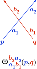
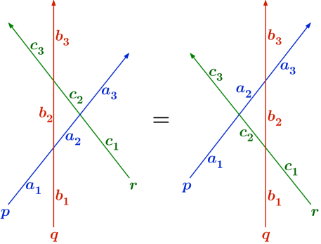
Figure 1: (Color online) Vertex-model Boltzmann weights (R-matrix) in graphical representation on the left and corresponding Yang–Baxter equation on the right. Here $a_{j},b_{j},c_{j}$ are state variables living on the edges and $p,q,r$ are line variables (rapidities). The states $a_{2},b_{2},c_{2}$ are summed over.

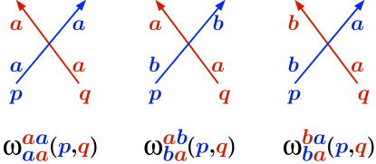
Figure 2: (Color online) The three types of non-zero Boltzmann weights of the sl$(m,n)$ vertex model of [17].

We change the variables according to

$$q\equiv\mathrm{e}^{2\eta},\quad x\equiv\mathrm{e}^{2q_{0}},\quad y\equiv\mathrm{e}^{2p_{0}},\quad\mathcal{N}\,{q^{1/2}\over\raise 1.0pt\hbox{$2$}}\Big{(}{y\over x}\Big{)}^{\!1/2}\!\equiv\mathcal{N}^{\prime},$$ (4)

in order to change the additive rapidities $p_{0}$ and $q_{0}$ to multiplicative rapidities $x$ and $y$. Thus we get

$$\boldsymbol{\omega}^{aa}_{aa}(p,q)=\cases{\mathcal{N}^{\prime}\Big{(}1-q^{-1}{\displaystyle{{x\over y}}}\Big{)}\displaystyle{p_{+a}q_{-a}\over q_{+a}p_{-a}},&if $\varepsilon_{a}=+1$,\cr\mathcal{N}^{\prime}\Big{(}{\displaystyle{{x\over y}}}-q^{-1}\Big{)}\displaystyle{p_{+a}q_{-a}\over q_{+a}p_{-a}},&if $\varepsilon_{a}=-1$,}$$ (5)

$$\boldsymbol{\omega}^{ab}_{ba}(p,q)=\mathcal{N}^{\prime}G_{ab}\,q^{-1/2}\Big{(}1-{\displaystyle{{x\over y}}}\Big{)}\displaystyle{p_{+a}q_{-a}\over q_{+a}p_{-a}},$$ (6)

$$\boldsymbol{\omega}^{ba}_{ba}(p,q)=\cases{\mathcal{N}^{\prime}(1-q^{-1}){\displaystyle{{x\over y}}}\displaystyle{p_{+b}q_{-a}\over q_{+b}p_{-a}},&if $a<b$,\cr\mathcal{N}^{\prime}(1-q^{-1})\displaystyle{p_{+b}q_{-a}\over q_{+b}p_{-a}},&if $a>b$.}$$ (7)

We reduce this to the root-of-unity case, if we set $\eta=j\pi\mathrm{i}/N$, or $q=\mathrm{e}^{2j\pi\mathrm{i}/N}$. When $j$ and $N$ are relative prime, $q$ is a primitive root of one. One can then proceed to cyclic representations of the quantum group $U_{q}(\widehat{\mathfrak{sl}}(n))$, provided one deals with the integer and half-integer powers of $q$ that may occur. The approach in [11] restricted $N$ to be odd, so that $q^{1/2}=-q^{(N+1)/2}$ and one only has integer powers of $q$ to deal with.

If $N\,\hbox{\mathaa\char 62\relax}\,3$, there is no choice of $p_{\pm a}$, $q_{\pm a}$ and $\mathcal{N}^{\prime}$ that can eliminate the half-integer powers of $q$. So, let us set $p_{\pm a}=q_{\pm a}\equiv 1,(a\neq 0),$ and $\mathcal{N}^{\prime}\equiv 1$. Then we arrive at

$$\boldsymbol{\omega}^{aa}_{aa}(p,q)=\cases{1-q^{-1}{\displaystyle{{x\over y}}},&if $\varepsilon_{a}=+1$,\cr{\displaystyle{{x\over y}}}-q^{-1},&if $\varepsilon_{a}=-1$,}$$ (8)

$$\boldsymbol{\omega}^{ab}_{ba}(p,q)=G_{ab}\,q^{-1/2}\Big{(}1-{\displaystyle{{x\over y}}}\Big{)}=\cases{1-{\displaystyle{{x\over y}}},&if $a>b$,\cr q^{-1}\Big{(}1-{\displaystyle{{x\over y}}}\Big{)},&if $a<b$,}$$ (9)

$$\boldsymbol{\omega}^{ba}_{ba}(p,q)=\cases{(1-q^{-1}){\displaystyle{{x\over y}}},&if $a<b$,\cr 1-q^{-1},&if $a>b$,}$$ (10)

provided we also choose $G_{ab}=q^{\pm{\rm sign}(a-b)/2}$, ($G_{ab}G_{ba}=1$), in (9). Then any $\boldsymbol{\omega}_{ab}^{cd}(p,q)$ is a linear combination of $1,q^{-1},{\textstyle{{x\over y}}},q^{-1}{\textstyle{{x\over y}}}$ only! This is how [12] overcame the odd-even $N$ problem, albeit that they have not spelled this out so explicitly.

Just choosing a more asymmetric R-matrix, or equivalently a different coproduct, one can treat the even and odd $N$ cases in a uniform way. This was also noted in [3] for the $n=2$ case, with the fundamental R-matrix the one of the 2-state six-vertex model.

3 Integrable chiral Potts model

The $N$-state integrable chiral Potts model is defined by its Boltzmann weights [2],

$${W_{pq}(n)\over W_{pq}(0)}=\prod_{j=1}^{n}\,{d_{p}b_{q}-a_{p}c_{q}\omega^{j}\over b_{p}d_{q}-c_{p}a_{q}\omega^{j}},\quad\displaystyle{{\overline{W}}_{pq}(n)\over{\overline{W}}_{pq}(0)}=\prod_{j=1}^{n}\,{\omega a_{p}d_{q}-d_{p}a_{q}\omega^{j}\over c_{p}b_{q}-b_{p}c_{q}\omega^{j}},$$ (11)

see also Fig. 3. Here the rapidities $p=(a_{p},b_{p},c_{p},d_{p})$ and $q=(a_{q},b_{q},c_{q},d_{q})$ live on the chiral Potts curve:

$$a_{p}^{\,N}+k^{\prime}b_{p}^{\,N}=k\,d_{p}^{\,N},\quad k^{\prime}a_{p}^{\,N}+b_{p}^{\,N}=k\,c_{p}^{\,N},\quad k^{2}+k^{\prime}{}^{2}=1,\quad\omega\equiv\mathrm{e}^{2\pi\mathrm{i}/N}.$$ (12)

These Boltzmann weights satisfy the star-triangle equation represented in Fig. 4, see the appendix of [19].

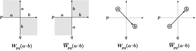
Figure 3: Graphical representation of the two types of chiral Potts Boltzmann weights with spin states $a,b=1,\ldots,N$ and oriented rapidity lines $p,q$. Both the checkerboard vertex model (left) and spin model (right) representations are given.

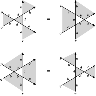
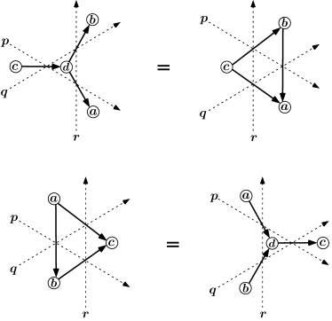
Figure 4: Graphical representations of the checkerboard Yang–Baxter equation on the left and the equivalent star-triangle equation on the right.

Combining four chiral Potts Boltzmann weights as a diamond or a star as in Fig. 5, we get R-matrices satisfying the uniform Yang–Baxter equation, so that we can forget about the checkerboard shading. Bazhanov and Stroganov [5] used the diamond map to relate chiral Potts with the six-vertex model for $N=\,$odd. Baxter, Bazhanov and Perk [6] used the star map instead to relate chiral Potts with the six-vertex model for all $N$. Their resulting interaction-round-a-face (IRF) model can be mapped to a vertex model, see $\mathsf{R}_{\mathrm{4CP}}$ in Fig. 6, using a Wu-Kadanoff-Wegner map [20, 21], putting now the differences $n_{1}=a-b$, $n_{2}=d-c$, $n_{3}=a-d$, $n_{4}=b-c$ (mod $N$) on the four edges.

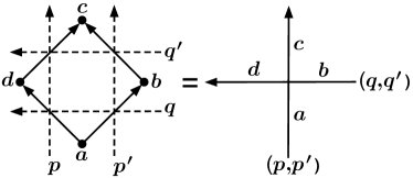
Figure 5: The diamond (left) and the star (right) of four Boltzmann weights.

In quantum-group representation theory, the fundamental R-matrix $\mathsf{R}_{\mathrm{6v}}$ intertwines two spin-${1\over 2}$ representations and $\mathsf{R}_{\mathrm{4CP}}$ intertwines two (minimal) cyclic representations. We need one more R-matrix $\mathsf{R}_{\tau_{2}}$ interwining the two different types of representations, see Fig. 6. This R-matrix generates what is now often called a $\tau_{2}$ model, a name going back to [5, 6], where a spin-$S$ representation intertwined with a cyclic representation corresponds with a $\tau_{2S+1}$ transfer matrix.

Figure 6: The three kinds of R-matrices to be used. Here all $\sigma_{i}=0,1$, correspond to the spin-$1\over 2$ representation, whereas all $n_{i}=0,\cdots,N\!-\!1$, i.e. $n_{i}\in\mathbb{Z}_{N}$, correspond to the cyclic representation.

The three R-matrices $\mathsf{R}_{\mathrm{6v}}$, $\mathsf{R}_{\tau_{2}}$ and $\mathsf{R}_{\mathrm{4CP}}$ satisfy a succession of four Yang–Baxter equations represented in Fig. 6. Here single rapidity lines correspond to spin-${1\over 2}$ representations of $\mathrm{U}_{q}({\widehat{\hbox{\bfrak sl}}}(2,\mathbb{C}))$, or quantum affine SL(2). Double rapidity lines carry two chiral Potts rapidities $(p,p^{\prime})$ and correspond to a minimal cyclic representation of $\mathrm{U}_{q}({\widehat{\hbox{\bfrak sl}}}(2,\mathbb{C}))$. This requires $q$ to be a root of unity, say $q=\omega=\mathrm{e}^{2\pi\mathrm{i}/N}$.

Figure 7: The four different Yang–Baxter equations.

4 The Boltzmann weights of the six-vertex model

The most general six-vertex model has six different weights as given in Fig. 8. This is the case $n=2$, $m=0$ of the previous section and now we can absorb the twisting factor $G_{ab}$ in (2) and the exponential factor ${\rm e}^{(p_{0}-q_{0}){\rm sign}(a-b)}$ in (3) into the gauge rapidities $p_{\pm i}$ and $q_{\pm i}$. We also go to the trigonometric representation replacing sinh by sin and we relabel the states $a,b=1,2$ as $\sigma,\sigma^{\prime}=0,1$. Different gauge choices lead to different $\tau_{2}$ models that have been connected with chiral Potts.

Figure 8: The six different six-vertex Boltzmann weights.

In the symmetric six-vertex model one has $a^{\prime}=a$, $b^{\prime}=b$, $c^{\prime}=c$. With this start Korepanov found a $\tau_{2}$ model, but no chiral Potts. To understand why, we parametrize the weights of the symmetric six-vertex model as

$$a=\mathcal{N}\sin(\eta+(v-u)),\quad b=\mathcal{N}\sin(v-u),\quad c=\mathcal{N}\sin(\eta),$$ (13)

with additive rapidities $u$ and $v$. There is also a multiplicative parametrization,

$$q\equiv\mathrm{e}^{2\mathrm{i}\eta},\quad x=\mathrm{e}^{2\mathrm{i}u},\quad y=\mathrm{e}^{2\mathrm{i}v},\quad\mathcal{C}=\mathcal{N}\,{q^{1/2}\over\raise 1.0pt\hbox{$2\mathrm{i}$}}\Big{(}{y\over x}\Big{)}^{\!1/2},$$ (14)

so that

$$a=\mathcal{C}\,\Big{(}1-q^{-1}{\displaystyle{{x\over y}}}\Big{)},\quad b=\mathcal{C}\,q^{-1/2}\Big{(}1-{\displaystyle{{x\over y}}}\Big{)},\quad c=\mathcal{C}\,\big{(}1-q^{-1}\big{)}\Big{(}{\displaystyle{{x\over y}}}\Big{)}^{\!1/2}.$$ (15)

If one sets $\eta=j\pi/N$, then one finds $q\equiv\mathrm{e}^{2\mathrm{i}\eta}=\mathrm{e}^{2j\pi\mathrm{i}/N}$, the root-of-unity case, which is one way to arrive at cyclic representations of quantum groups. However, the symmetric gauge is not a good start for the fundamental representation of sl(2) quantum: The square root $\sqrt{x/y}$ makes things ugly and it could have been eliminated by a gauge transformation. Up to normalization $\mathcal{C}$ the R-matrix used by Korepanov is

$$\mathsf{R}_{\mathrm{sym}}(x,y)=\pmatrix{1-{\displaystyle{{x\over y}}}q^{-1}&0&0&0\cr 0&\Big{(}1-{\displaystyle{{x\over y}}}\Big{)}\,q^{-1/2}&\Big{(}{\displaystyle{{x\over y}}}\Big{)}^{\!1/2}(1-q^{-1})&0\cr 0&\Big{(}{\displaystyle{{x\over y}}}\Big{)}^{\!1/2}(1-q^{-1})&\Big{(}1-{\displaystyle{{x\over y}}}\Big{)}\,q^{-1/2}&0\cr 0&0&0&1-{\displaystyle{{x\over y}}}q^{-1}}.$$ (16)

The $\big{(}x/y)^{1/2}$ and $q^{-1/2}$ cause complications especially for $N$ even.

Bazhanov and Stroganov [5] used the asymmetric gauge typically used in quantum group theory,

$$\mathsf{R}_{\mathrm{B\&S}}(x,y)=\pmatrix{1-{\displaystyle{{x\over y}}}q^{-1}&0&0&0\cr 0&\Big{(}1-{\displaystyle{{x\over y}}}\Big{)}\,q^{-1/2}&{\displaystyle{{x\over y}}}(1-q^{-1})&0\cr 0&1-q^{-1}&\Big{(}1-{\displaystyle{{x\over y}}}\Big{)}\,q^{-1/2}&0\cr 0&0&0&1-{\displaystyle{{x\over y}}}q^{-1}}.$$ (17)

They were able to arrive at the chiral Potts model only for $N$ odd. Now the $q^{-1/2}$ still causes complications for $N$ even, just like in the more general $n\,\hbox{\mathaa\char 62\relax}\,2$ case of section 2.

A more asymmetric gauge was found in [6] starting from the chiral Potts side,

$$\mathsf{R}_{\mathrm{BBP}}(x,y)=\pmatrix{1-{\displaystyle{{x\over y}}}q^{-1}&0&0&0\cr 0&1-{\displaystyle{{x\over y}}}&{\displaystyle{{x\over y}}}(1-q^{-1})&0\cr 0&1-q^{-1}&\Big{(}1-{\displaystyle{{x\over y}}}\Big{)}q^{-1}&0\cr 0&0&0&1-{\displaystyle{{x\over y}}}q^{-1}}.$$ (18)

This was already pointed out in [3]. As now only 1, $x/y$, $q^{-1}$, and $(x/y)q^{-1}$ show up, the situation is least complicated with the “smallest linear dimension.” The commutation relations of the four elements of the monodromy matrix are now least complicated [3].

5 Gauge Changes of Six-Vertex Boltzmann Weights

In order to understand how the three approaches relate, we start with $\mathsf{R}_{\mathrm{BBP}}$ and apply suitable gauge transforms of the two types in Fig. 9.

Figure 9: (a) Staggered gauge transform. (b) Uniform gauge transform.

A staggered gauge transform with $\mathsf{G}$ of the simple diagonal form

$$\mathsf{G}=\pmatrix{\lambda&0\cr 0&\lambda^{-1}},\quad\mbox{with}\quad\lambda=q^{1/8},$$ (19)

can be used to connect $\mathsf{R}_{\mathrm{B\&S}}$ and $\mathsf{R}_{\mathrm{BBP}}$ in each of two different ways given in Fig. 9(a). A uniform gauge transform

$$\mathsf{G}=\pmatrix{\lambda&0\cr 0&\lambda^{-1}},\quad\mbox{with}\quad\lambda=\Big{(}{x\over y}\Big{)}^{1/8},$$ (20)

as in Fig. 9(b) connects $\mathsf{R}_{\mathrm{sym}}$ and $\mathsf{R}_{\mathrm{B\&S}}$.

In the approach of BBP [6] there is no difficulty with even roots of unity. However, the staggered gauge transforms to the Bazhanov–Stroganov approach, and then also to the Korepanov symmetric gauge, lead to complications: Two distinct $\tau_{2}$ matrices arise in the $\mathsf{R}_{\mathrm{6v}}\mathsf{R}_{\tau_{2}}\mathsf{R}_{\tau_{2}}$ Yang–Baxter equation of Fig 7.

It may be said that Korepanov [9, 10] during 1986–1987 has made some start to solve the even root-of-unity problem using two $\tau_{2}$ matrices. He solved the $\mathsf{R}_{\mathrm{6v}}\mathsf{R}_{mathrm{6v}}\mathsf{R}_{\tau_{2}}$ Yang–Baxter equation of Fig 7 using $\mathsf{R}_{\mathrm{sym}}$, giving one $\mathsf{R}_{\tau_{2}}$ for $N=\,$odd, while for $N=\,$ even his solution has two different $\mathsf{R}_{\tau_{2}}$. However, he did not address the next steps in Fig 7, so that he could not arrive at the chiral Potts model.

Bazhanov and Stroganov did address the next steps in the succession of Yang–Baxter equations, starting with $\mathsf{R}_{\mathrm{B\&S}}$, which is the typical choice for the intertwiner of two fundamental representations of $\mathrm{U}_{q}({\widehat{\hbox{\bfrak sl}}}(2,\mathbb{C}))$. However, to explicitly represent $\mathsf{R}_{\tau_{2}}$ for $q=\omega\equiv\mathrm{e}^{2\pi\mathrm{i}/N}$, they introduce $q_{1}^{\vphantom{y}}=q^{(N+1)/2}$, satisfying $q_{1}^{N}=1$, $q=q_{1}^{-2}$, which can only be done for $N=\,$odd. For $N=\,$even, both solutions $q_{1}^{\vphantom{y}}$ of $q_{1}^{\,2}=q$ satisfy $q_{1}^{N}=-1$.

Finally, the two approaches of B&S and BBP lead to different $q$-Pochhammer symbols, as explained in [3], namely

$$[a;q_{1}]_{n}=\prod_{k=1}^{n}(a^{-1}q_{1}^{n-1}-aq_{1}^{1-n})\quad\hbox{versus}\quad(a;q)_{n}=\prod_{k=1}^{n}(1-aq^{n-1}),$$ (21)

and also different $q$-integers,

$$[q_{1}]_{n}={q_{1}^{n}-q_{1}^{-n}\over q_{1}^{\vphantom{y}}-q_{1}^{-1}}\quad\hbox{versus}\quad\displaystyle(q)_{n}={1-q^{n}\over 1-q}.$$ (22)

The approach of [6] leads to more standard notations of the theory of basic hypergeometric functions.

References

References

• [1] Au-Yang H, McCoy B M, Perk J H H, Tang S and Yan M-L 1987 Commuting transfer matrices in the chiral Potts models: Solutions of the star-triangle equations with genus $>1$ Phys. Lett. A 123 219–23
• [2] Baxter R J, Au-Yang H and Perk J H H 1988 New solutions of the star-triangle relations for the chiral Potts model Phys. Lett. A 128 138–42
• [3] Perk J H H 2016 The early history of the integrable chiral Potts model and the odd-even problem J. Phys. A: Math. Theor. 49 153001 (20pp) (arXiv:1511.08526)
• [4] De Concini C and Kac V G 1990 Representations of quantum groups at roots of 1 Operator Algebras, Unitary Representations, Enveloping Algebras, and Invariant Theory: Actes du Colloque en l’Honneur de Jacques Dixmier (Progress in Mathematics vol 92) ed Connes A, Duflo M, Joseph A and Rentschler R (Boston, MA: BirkhΓ€user) ppΒ 471–506
• [5] Bazhanov V V and Stroganov Yu G 1990 Chiral Potts model as a descendant of the six-vertex model J. Stat. Phys. 59 799–817
• [6] Baxter R J, Bazhanov V V and Perk J H H 1990 Functional relations for transfer matrices of the chiral Potts model Intern. J. Mod. Phys. B 4 803–70
• [7] Au-Yang H and Perk J H H 2016 CSOS models descending from chiral Potts models: Degeneracy of the eigenspace and loop algebra J. Phys. A: Math. Theor. 49 154003 (arXiv:1511.08523)
• [8] Maillet J M, Niccoli G and Pezelier B 2018 Transfer matrix spectrum for cyclic representations of the 6-vertex reflection algebra II arXiv:1802.08853
• [9] Korepanov I G 1994 Hidden symmetries in the 6-vertex model of statistical physics Zap. Nauch. Sem. POMI 215 163–77 [English translation: J. Math. Sc. 85 1661–70 (1997)] (arXiv:hep-th/9410066)
• [10] Korepanov I G 1994 Vacuum curves of $\mathcal{L}$-operators associated with the six-vertex model Algebra i Analiz 6:2 176–94 [English translation: St. Petersburg Math. J. 6:2 349–64 (1995)]
• [11] Date E, Jimbo M, Miki M and Miwa T 1991 Generalized Chiral Potts Models and Minimal Cyclic Representations of $U_{q}(\widehat{\mathfrak{gl}}(n,\mathrm{C}))$ Commun. Math. Phys. 137 133–47
• [12] Bazhanov V V, Kashaev R M, Mangazeev V V and Stroganov Yu G 1991 $(Z_{N}\,\times\,)^{n-1}$ Generalization of the Chirai Potts Model Commun. Math. Phys. 138 393–408
• [13] Fendley P 2014 Free parafermions J. Phys. A: Math. Theor. 47 075001 (42pp) (arXiv:1310.6049)
• [14] Baxter R J 2014 The $\tau_{2}$ model and parafermions J. Phys. A: Math. Theor. 47 315001 (12pp) (arXiv:1310.7074)
• [15] Au-Yang H and Perk J H H 2014 Parafermions in the $\tau_{2}$ model J. Phys. A: Math. Theor. 47 315002 (19pp) (arXiv:1402.0061)
• [16] Au-Yang H and Perk J H H 2016 Parafermions in the $\tau_{2}$ model II arXiv:1606.06319
• [17] Perk J H H and Schultz C L 1981 New families of commuting transfer matrices in $q$-state vertex models Phys. Lett. A 84 407–10
• [18] Perk J H H and Au-Yang H 2006 Yang–Baxter Equation Encyclopedia of Mathematical Physics volΒ 5 ed FranΓ§oise J-P, Naber G L and Tsou S T (Oxford: Elsevier Science) ppΒ 465–73 (extended version: arXiv:math-ph/0606053)
• [19] Au-Yang H and Perk J H H 1989 Onsager’s star-triangle equation: Master key to integrability Integrable Systems in Quantum Field Theory and Statistical Mechanics (Advanced Studies in Pure Mathematics vol 19) ed Jimbo M, Miwa T and Tsuchiya A (Tokyo: Kinokuniya-Academic) ppΒ 57–94, appendix
• [20] Wu F Y 1971 Ising model with four-spin interactions Phys. Rev. B 4 (1971), 2312–4
• [21] Kadanoff L P and Wegner F J 1971 Some critical properties of the eight-vertex model Phys. Rev. B 4 3989–93
• [22] Baxter R J 2004 Transfer matrix functional relations for the generalized $\tau_{2}(t_{q})$ model J.Β Stat.Β Phys. 117 1–25 (arXiv:cond-mat/0409493)