CONSTRAINTS ON THE DISTANCE MODULI, HELIUM AND METAL ABUNDANCES, AND AGES OF GLOBULAR CLUSTERS FROM THEIR RR LYRAE AND NON-VARIABLE HORIZONTAL-BRANCH STARS. III. M 55 AND NGC 6362

Abstract

M 55 (NGC 6809) and NGC 6362 are among the few globular clusters for which masses and radii have been derived to high precision for member binary stars. They also contain RR Lyrae variables which, together with their non-variable horizontal-branch (HB) populations, provide tight constraints on the cluster reddenings and distance moduli through fits of stellar models to their pulsational and evolutionary properties. Reliable $(m-M)_{V}$ estimates yield $M_{V}$ and $M_{\rm bol}$ values of comparable accuracy for binary stars because the $V$-band bolometric corrections applicable to them have no more than a weak dependence on effective temperature (${T_{\rm eff}}$) and [Fe/H]. Chemical abundances derived from the binary mass–$M_{V}$ relations are independent of determinations based on their spectra. The temperatures of the binaries, which are calculated directly from their luminosities and the measured radii, completely rule out the low ${T_{\rm eff}}$ scale that has been determined for metal-deficient stars in some recent spectroscopic and interferometric studies. If [$\alpha$/Fe] $=0.4$ and [O/Fe] $=0.5\pm 0.1$, we find that M 55 has $(m-M)_{V}=13.95\pm 0.05$, [Fe/H] $=-1.85\pm 0.1$, and an age of $12.9\pm 0.8$ Gyr, whereas NGC 6362 has $(m-M)_{V}=14.56\pm 0.05$, [Fe/H] $=-0.90\pm 0.1$, and an age of $12.4\pm 0.8$ Gyr. The HB of NGC 6362 shows clear evidence for multiple stellar populations. Constraints from the RR Lyrae standard candle and from local subdwarfs (with Gaia DR2 parallaxes) are briefly discussed.

1. Introduction

More than 60 years have passed since photometry derived from photographic plates taken at the 200-inch telescope on Mt. Palomar revealed for the first time the turnoffs of globular clusters (GCs) — specifically, those of M 92 (Arp et al. 1953) and M 3 (Sandage 1953). During the following decade, color-magnitude diagrams (CMDs) extending down to the main sequence (MS) were obtained for several other GCs, including M 13 (Baum et al. 1959), M 5 (Arp 1962), and 47 Tuc (Tifft 1963). Interestingly, the basic properties of these clusters that were derived for them (in particular, their distances and metallicities) are closer to present-day determinations than one might have expected.

For instance, most of the pioneering studies mentioned in the previous paragraph argued in support of the apparent distance moduli, $(m-M)_{V}$, that were obtained if RR Lyrae variables were assumed to have $M_{V}\approx 0.6$. This was supported, in part, by the determination of $M_{V}=0.65\pm 0.1$ for RR Lyr itself from the application of the moving-group method (see Eggen & Sandage 1959). However, Sandage (1958) suspected early on that cluster-to-cluster variations in the mean periods of the RR Lyrae could be explained if the luminosity of the horizontal branch (HB) increased with decreasing metallicity. Subsequently, Sandage & Wallerstein (1960) suggested that it would be reasonable to place the HB at $M_{V}=0.4$ in M 92, at $M_{V}=0.6$ in M 3 (to be consistent with RR Lyr), and at fainter absolute magnitudes in more metal-rich systems. As it turns out, distance moduli inferred from recent models for the HB phase imply $\langle M_{V}\rangle=0.35$ and 0.58 for M 92 and M 3, respectively (see Table 1 in VandenBerg et al. 2016, hereafter Paper I), which agree with the results from the Sandage & Wallerstein paper to within several hundredths of a magnitude.

Indeed, the main advance during the intervening years has been to reduce the uncertainties associated with the derived $(m-M)_{V}$ values from $\sim\pm 0.2$–0.3 mag (e.g., Baum et al. 1959, Tifft 1963) to $\sim\pm 0.1$ mag. In well observed clusters such as M 92, M 5, and 47 Tuc, the $1\,\sigma$ uncertainties appear to be somewhat less than this; see Table 1, which lists many of the apparent distance moduli that have been derived for these three clusters since the turn of the century. As indicated in the second column, some studies used local subdwarf (SBDWF) or subgiant branch (SGB) stars, RR Lyrae (RRL), or white dwarfs (WD) as standard candles. Others constrained the cluster distances using luminosity functions (LFs), red-giant (RG) clump or tip stars, eclipsing binary members, RR Lyrae period-luminosity (PL) relations, theoretical results that give the RR Lyrae pulsation period as a function of its mass, luminosity, effective temperature, and metallicity (${\cal M}L{T_{\rm eff}}Z$), or detailed comparisons between synthetic and observed HB populations (“HB fits”). Some of the earliest estimates of $(m-M)_{V}$ — e.g., 14.62 for M 92 by Sandage & Walker (1966), 14.39 for M 5 by Arp (1962), and 13.35 for 47 Tuc by Tifft (1963) — clearly agree quite well with the tabulated values.

Table 1Determinations of $(m-M)_{V}$ for M 92, M 5, and 47 Tuc

Reference	Method	$(m-M)_{V}$
M 92
Carretta et al. (2000)	SBDWF	14.72
VandenBerg (2000)	ZAHB	14.70
VandenBerg et al. (2002)	SGB	14.62
Del Principe et al. (2005)	RRL (PL)	14.67
Sollima et al. (2006)	RRL (PL)	14.73
Paust et al. (2007)	LFs	14.66
An et al. (2009)	SBDWF	14.71
Benedict et al. (2011)	RRL	14.78
VandenBerg et al. (2013)	ZAHB	14.72
VandenBerg et al. (2016)	RRL (${\cal M}L{T_{\rm eff}}Z$)	14.74
Chaboyer et al. (2017)	SBDWF	14.89
Average($\sigma$)		$14.72(0.07)$
M 5
Carretta et al. (2000)	SBDWF	14.57
VandenBerg (2000)	ZAHB	14.48
Di Criscienzo et al. (2004)	RRL (${\cal M}L{T_{\rm eff}}Z$)	14.41
Layden et al. (2005)	SBDWF	14.56
Sollima et al. (2006)	RRL (PL)	14.46
An et al. (2009)	SBDWF	14.40
Coppola et al. (2011)	RRL (PL)	14.53
VandenBerg et al. (2013)	ZAHB	14.38
VandenBerg et al. (2014b)	SBDWF	14.40
Arellano Ferro et al. (2016)	RRL (PL)	14.49
Average($\sigma$)		$14.47(0.07)$
47 Tuc
Carretta et al. (2000)	SBDWF	13.55
VandenBerg (2000)	ZAHB	13.37
Ferraro et al. (2000)	RG tip	13.44
Zoccali et al. (2001)	WD	13.27
Percival et al. (2002)	SBDWF	13.37
Grundahl et al. (2002)	SBDWF	13.33
Salaris & Girardi (2002)	RG clump	13.34
Bergbusch & Stetson (2009)	SBDWF	13.38
Thompson et al. (2010)	binary	13.35
Salaris et al. (2016)	HB fits	13.40
Denissenkov et al. (2017)	HB fits	13.27
Brogaard et al. (2017)	binary	13.30
Average($\sigma$)		$13.37(0.08)$

Similarly, the overall metallicities that were derived for GCs in the 1960s seem quite reasonable from today’s perspective, even though little was known about the detailed metals mixtures at the time. For example, based on measurements of the ultraviolet excesses in cluster stars, Arp (1962) concluded that the metals-to-hydrogen ($M$/H) ratios in M 92 and M 5 differed from the solar value by, in turn, factors of $\mathrel{\hbox{\raise 2.58334pt\hbox{$<$}\kern-7.74998pt\lower 2.15277pt\hbox{$\sim$}}}1/200$ and $\sim 1/17$, whereas spectra of individual giants in 47 Tuc implied a factor $\mathrel{\hbox{\raise 2.58334pt\hbox{$>$}\kern-7.3194pt\lower 2.15277pt\hbox{$\sim$}}}1/4$ (Feast & Thackeray 1960). In the usual logarithmic notation, the corresponding [$M$/H] values are $-2.3$, $-1.2$, and $-0.6$, which are $\mathrel{\hbox{\raise 2.58334pt\hbox{$<$}\kern-7.74998pt\lower 2.15277pt\hbox{$\sim$}}}0.15$ dex higher than the [Fe/H] values that have been obtained in modern spectroscopic studies for M 92, M 5, and 47 Tuc, respectively (e.g., Carretta & Gratton 1997; Kraft & Ivans 2003; Carretta et al. 2009a, hereafter CBG09). (Differences of a similar amount, but in the opposite sense, are implied by current [$M$/H] values that take into account enhanced abundances of the $\alpha$-elements by 0.3–0.4 dex.)

However, despite the vast amount of spectroscopic work that has been carried out over the years (see, e.g., the compilations of published results by Pritzl et al. 2005, Roediger et al. 2014), the uncertainties associated with the absolute abundances of many metals remain large. This is illustrated in Figure 1, which shows that the [Fe/H] values derived by Carretta & Gratton (1997, hereafter CG97) tend to be $\mathrel{\hbox{\raise 2.58334pt\hbox{$>$}\kern-7.3194pt\lower 2.15277pt\hbox{$\sim$}}}0.2$ dex larger than those found by Kraft & Ivans (2003, hereafter KI03), except at the metal-rich end. High-resolution spectra were used in both investigations, but Kraft & Ivans anchored their determinations to [Fe/H] values based on Fe II lines to minimize the effects of possible departures from local thermodynamic equilibrium (LTE), whereas neutral iron lines provided the basis of the CG97 metallicity scale. A recalibration of the latter by CBG09, using even higher resolution spectra, improved $gf$ values, and a somewhat cooler ${T_{\rm eff}}$ scale, resulted in [Fe/H] determinations that agreed reasonably well with those by KI03, though differences at the level of 0.1–0.2 dex persisted for many clusters (note the vertical separations between the pairs of open and filled circles in Fig. 1).

Figure 1.— Comparison of the [Fe/H] values for 23 globular clusters derived by Carretta & Gratton (1997, CG97) with those given by Kraft & Ivans (2003, KI03, filled circles), CBG09 (open circles), and recent studies (crosses) of M 15 (Sobeck et al. 2011), M 92 (Roederer & Sneden 2011), and NGC 4833 (Roederer & Thompson 2015). Note that the vertical offsets of some of the points from the diagonal “line of equality” are $\mathrel{\hbox{\raise 2.58334pt\hbox{$>$}\kern-7.3194pt\lower 2.15277pt\hbox{$\sim$}}}0.6$ dex.

Unfortunately, even more recent spectroscopic studies have tended to “muddy the water”. The latest results for M 15 (Sobeck et al. 2011), M 92 (Roederer & Sneden 2011), and NGC 4833 (Roederer & Thompson 2015), which have been plotted as crosses in Fig. 1, are $\sim 0.3$ dex lower than the CBG09 determinations, and $\sim 0.6$ dex less than the values reported by CG97. As discussed by Roederer & Sneden, the factor of two reduction in the iron abundances relative to the findings that some of the same authors had previously obtained (e.g., Sneden et al. 2000) appears to be due to differences in (i) the Fe I lines that were selected for analysis, (ii) the adopted $gf$ values, (iii) the treatment of the Rayleigh scattering component of the blue continuous opacity, and (iv) the 1D model atmospheres that were employed.

Even when extremely high quality spectra are available, as in the case of nearby halo stars with well determined distances, the [Fe/H] values derived from their spectra can vary by $>0.3$ dex. This is exemplified by recent work on the turnoff (TO) star HD 84937, for which Amarsi et al. (2016) obtained [Fe/H] $=-1.96$ from detailed 3D, non-LTE radiative transfer calculations, as compared with the value of [Fe/H] $=-2.32$ that was found by Sneden et al. (2016) using 1D model atmospheres. (The latter argue that there are no substantial departures from LTE in this star; for additional discussion on this point and possible concerns with 3D model atmospheres at low metallicities, see Spite et al. 2017.)

Table 2Properties of HD 84937

Reference	$\log\,g$	$T_{\rm eff}$	[Fe/H]
Gratton et al. (1996)	4.06	6344	$-2.04$
Jonsell et al. (2005)	4.04	6310	$-1.96$
Gehren et al. (2006)	4.00	6346	$-2.16$
Cenarro et al. (2007)	4.01	6228	$-2.17$
Mashonkina et al. (2008)	4.00	6365	$-2.15$
Casagrande et al. (2010)	3.93	6408	$-2.11$
Bergemann et al. (2012)	4.13	6408	$-2.16$
Ramírez et al. (2013)	4.15	6377	$-2.02$
VandenBerg et al. (2014b)	4.05	6408	$-2.08$
Sitnova et al. (2015)	4.09	6350	$-2.12$
Amarsi et al. (2016)	4.06	6356	$-1.96$
Sneden et al. (2016)	4.00	6300	$-2.32$

Most studies of HD 84937 over the past two decades have found intermediate [Fe/H] values — as shown in Table 2, which lists only a representative fraction ($\mathrel{\hbox{\raise 2.58334pt\hbox{$<$}\kern-7.74998pt\lower 2.15277pt\hbox{$\sim$}}}50$%) of the investigations that considered this star during the past two decades. Although the metallicity that was reported in any one of the tabulated papers has some dependence on the adopted temperature, the ${T_{\rm eff}}$ value seems to be less important than other ingredients of chemical abundance determinations (model atmospheres, atomic physics, etc.). For instance, some of the studies referenced in Table 2 adopted nearly the same ${T_{\rm eff}}$ values and yet their [Fe/H] determinations differ by $>0.3$ dex (see the entries for Jonsell et al. 2005, Sneden et al. 2016), while others found nearly the same metallicities, despite assuming very different temperatures (e.g., Cenarro et al. 2007, Bergemann et al. 2012). Judging from the discordant results that were published $\sim 2$ years ago (Amarsi et al. 2016, Sneden et al. 2016), it may be some time before we can claim that the absolute metallicity of HD 84937 is known to better than 0.1 dex. (Considering just the tabulated findings, the average [Fe/H] value is $-2.10$, with a $1\,\sigma$ standard deviation from the mean of 0.10 dex.)

At the present time, the relatively high temperatures that are found from the application of the infrared flux method (IRFM; see, e.g., Casagrande et al. 2010, hereafter CRMBA; Meléndez et al. 2010) seem to be favored (also from the theoretical perspective; see the overlays of isochrones onto the CMD locations of nearby subdwarfs by VandenBerg et al. 2010), but this issue is not yet settled. As shown by CRMBA, IRFM temperatures agree reasonably well with those derived from the hydrogen lines by Bergemann (2008) and Fabbian et al. (2009), except at ${T_{\rm eff}}\mathrel{\hbox{\raise 2.58334pt\hbox{$>$}\kern-7.3194pt\lower 2.15277pt\hbox{$\sim$}}}6100$ K where they are hotter by $\sim 50$–100 K. The recent analysis of interferometric data for the nearby, [Fe/H] $\sim-2.4$ subgiant, HD 140283, by Creevey et al. (2015) may also be a potential problem for the IRFM ${T_{\rm eff}}$ scale, but as discussed in their paper, stellar models would require a very low value of the mixing-length parameter ($\alpha_{\rm MLT}$) in order to explain their observations. This would be at odds with the implications of globular cluster CMDs for $\alpha_{\rm MLT}$ (see Paper I) as well as recent calibrations of the mixing-length parameter based on 3D hydrodynamical model atmospheres (Magic et al. 2015). Consequently, it is not clear whether HD 140283 has anomalous properties or the temperature derived for it by Creevey et al. is too low. In any case, even if the IRFM ${T_{\rm eff}}$ scale is trustworthy, the typical uncertainties of $\sim\pm 70$ K for a given star still imply a range of most probable values that spans nearly 150 K.

Uncertainties associated with stellar temperatures and absolute [Fe/H] values (as well as [O/H], [Mg/H], etc.; see, e.g., Fabbian et al. 2009; Ramírez et al. 2013; Bergemann et al. 2012, ; Zhao et al. 2016, and references therein), which appear to range from $\sim\pm 0.1$–0.25 dex (especially at the lowest metallicities), obviously limit our ability to test and to improve stellar models. (Much higher precisions are quoted in most abundance determinations, but the stated uncertainties will not have taken into account the errors associated with such things as the assumed atmospheric temperature structures, the adopted atomic physics, and the evaluation of non-LTE effects, which are not easily determined.) Discrepancies between predicted and observed CMDs, for instance, can easily be due to problems with the predicted ${T_{\rm eff}}$ values, given that they are very dependent on the treatment of convection and the atmospheric boundary condition (see, e.g., VandenBerg et al. 2008, 2014). However, it is also possible that errors in the photometry, the adopted color–${T_{\rm eff}}$ relations, and/or the assumed cluster properties (reddening, distance, chemical abundances) are responsible. Unless the basic properties of the stars are known to high accuracy, it is very difficult to evaluate, e.g., the reliability of different color transformations, the extent to which $\alpha_{\rm MLT}$ varies with mass, metallicity, or evolutionary state, etc.

Tightening the constraints on the empirical metallicity and ${T_{\rm eff}}$ scales would certainly help to break through the current impasse. The presence of detached, eclipsing binaries in GCs that also contain RR Lyrae provides an avenue for doing just that. Normally, binaries have been used to obtain an independent estimate of the age and distance modulus of a given GC on the assumption of spectroscopically derived abundances and temperatures of the components that are usually inferred from their colors (see, e.g., Thompson et al. 2010, Kaluzny et al. 2013). Although distance-independent ages can be derived from the binary mass–radius and mass–$M_{V}$ relations, they are not particularly well constrained because the predicted radii depend on uncertain model temperatures, and the luminosities of the binary components, from which their $M_{V}$ values are calculated, depend on the uncertain ${T_{\rm eff}}$ values that are adopted for them. This has been demonstrated in the study of the 47 Tuc binary, V69, by Brogaard et al. (2017), who have also shown that the helium and metal abundances are important variables in such analyses, because lower $Y$ has similar effects on mass–radius and mass–luminosity relations at a fixed age as increased [Fe/H] and/or [O/Fe].

Previous papers in the present series have given us considerable confidence that accurate distances of GCs, especially those that contain RR Lyrae variables, can be determined from state-of-the-art HB models. To be more specific, we showed in Paper I that the observed periods of the RR Lyrae in M 3, M 15, and M 92 agree very well with those predicted by modern HB tracks on the assumption of distance moduli that are obtained from fits of ZAHB models to the non-variable HB populations of each cluster. The distance modulus obtained in this way for M 3, in particular, is in excellent agreement with that implied by the best available calibration of the RR Lyrae standard candle at [Fe/H] $\sim-1.5$. Moreover, the synthetic HB populations that were generated by Denissenkov et al. (2017, hereafter Paper II) provided very realistic reproductions of the observed distributions of HB stars in M 3, M 13, and 47 Tuc, if the helium abundance varies by $\delta Y\approx 0.02$, 0.08, and 0.03, respectively. Thus, HB models are able to place tight limits on He abundance variations within GCs (as already demonstrated by, e.g., Salaris et al. 2016), as well as on their distances.

Such results are not particularly dependent on the adopted metallicities. That is, assuming a higher or lower [Fe/H] by $\mathrel{\hbox{\raise 2.58334pt\hbox{$<$}\kern-7.74998pt\lower 2.15277pt\hbox{$\sim$}}}0.2$ dex would entail an adjustment of the ZAHB-based distance modulus by only $\mathrel{\hbox{\raise 2.58334pt\hbox{$<$}\kern-7.74998pt\lower 2.15277pt\hbox{$\sim$}}}\pm 0.04$ mag, and simply by making a small, compensating offset of the model ${T_{\rm eff}}$ scale (by $\delta\log{T_{\rm eff}}\mathrel{\hbox{\raise 2.58334pt\hbox{$<$}\kern-7.74998pt\lower 2.15277pt\hbox{$\sim$}}}0.004$), one would obtain essentially the same fit to the pulsational properties of the RR Lyrae. (The $\delta{T_{\rm eff}}$ estimate in this example is based on the reasonable assumptions that $\delta M_{\rm bol}\approx\delta M_{V}$, and that pulsational periods, which vary directly with luminosity but inversely with temperature, are nearly four times as dependent on $\log{T_{\rm eff}}$ as on $\log(L/L_{\odot})$; see Marconi et al. 2015.)

However, once the distance modulus is set, and the consequent TO age is determined, the isochrone for that age must be able to reproduce the binary mass–$M_{V}$ relation. In general, some iteration of the assumed abundances and/or the adopted value of $(m-M)_{V}$ will be necessary to achieve a consistent interpretation of both the member binaries and the cluster RR Lyrae (if, indeed, it is possible to do so). If consistency is obtained, then the effective temperatures of the binary components that are calculated directly from the measured radii and the derived luminosities will provide valuable constraints on the stellar ${T_{\rm eff}}$ scale at the [Fe/H] value of the GC under consideration.

In principle, detached, ecliping binaries in GCs provide a particularly promising way to determine the temperatures of metal-poor stars over a very wide range in [Fe/H]. Since the radii of their components can often be measured to within 1%, the uncertainties in the ${T_{\rm eff}}$ values that are derived from $L=4\pi R^{2}\sigma{T_{\rm eff}}^{4}$ are mainly limited by the accuracy of the intrinsic luminosities. In order for the temperatures derived in this way to be competitive with those based on alternative methods, it is necessary to know the distance modulus of the binary, and hence of the cluster that it resides in, to better than $\sim\pm 0.08$ mag, as this translates into $\delta\log{T_{\rm eff}}\approx\pm 0.01$ if $\delta R/R\sim 0.01$ and the errors in the apparent magnitudes are $\mathrel{\hbox{\raise 2.58334pt\hbox{$<$}\kern-7.74998pt\lower 2.15277pt\hbox{$\sim$}}}0.01$–0.02 mag. Moreover, binary mass-luminosity relations, which are nearly independent of model atmospheres and synthetic spectra (aside from the conversion of $M_{V}$ to $M_{\rm bol}$), provide an important constraint of the chemical abundances that are derived spectroscopically.

In this investigation, the approach described above is applied to the globular clusters M 55 (NGC 6809) and NGC 6362, which have iron abundances that differ by about a factor of 10 (see, e.g., CBG09). The masses and radii of the detached eclipsing binary in M 55 (known as V54) have been derived to within 2.1% and 0.95%, respectively, by Kaluzny et al. (2014). The same group (see Kaluzny et al. 2015) have been able to measure the masses of the components of two detached eclipsing binaries, V40 and V41, in NGC 6362 to better than $0.71$%, as compared with radius uncertainties of $<1.3$%. Mean magnitudes and colors of the 15 RR Lyrae variables that have been found in M 55 are provided by Olech et al. (1999), who also measured these quantities in the nearly three dozen RR Lyrae that reside in NGC 6362 (Olech et al. 2001).

The next section briefly describes the stellar models and additional theoretical results that are used in this work. Sections 3 and 4 contain, in turn, our analyses of the CMDs, the RR Lyrae populations, and the eclipsing binaries in M 55 and in NGC 6362. The implications of the distance moduli that we have determined from HB models for the calibration of the RR Lyrae standard candle is presented in section 5, where a fit of the M 55 main sequence to local subdwarfs is also reported and discussed. The main conclusions of this investigation are summarized in section 6.

2. Theoretical Considerations

All of the stellar evolutionary calculations considered in this paper adopt the solar mix of heavy elements given by Asplund et al. (2009) as the reference mixture. At the [Fe/H] values of interest, enhanced $\alpha$-element abundances by $+0.4$ dex have generally been assumed, which is consistent with the mean values of [Mg/Fe] and [Si/Fe] that have been derived in the spectroscopic study of 19 GCs, including M 55, by Carretta et al. (2009b). Although the latter find that oxygen is less enhanced, with $\langle$[O/Fe]$\rangle$ closer to $+0.2$ than to $+0.4$, star-to-star variations in the abundance of this element are typically $\mathrel{\hbox{\raise 2.58334pt\hbox{$>$}\kern-7.3194pt\lower 2.15277pt\hbox{$\sim$}}}0.4$ dex; e.g., for the clusters considered by Carretta et al. (see their Table 10), the mean rms variation of $\langle$[O/Fe]$\rangle$ is 0.18 dex. (Such variations are apparent in the ubiquitous O–Na anticorrelations that are widely considered to be one of the defining properties of GCs.) Since oxygen will be converted to nitrogen as the result of CNO-cycling at high temperatures, the highest O abundances, which are roughly consistent with [$\alpha$/Fe] $=+0.4$, are more likely to be representative of the initial abundance than the mean cluster abundance. In fact, [O/Fe] values in GCs with $-2.0\mathrel{\hbox{\raise 2.58334pt\hbox{$<$}\kern-7.74998pt\lower 2.15277pt\hbox{$\sim$}}}$ [Fe/H] $\mathrel{\hbox{\raise 2.58334pt\hbox{$<$}\kern-7.74998pt\lower 2.15277pt\hbox{$\sim$}}}-0.8$ could be as high as $\sim+0.6$ if their CN-weak populations have the same oxygen abundances as field stars with similar metallicities (see, e.g., Fabbian et al. 2009; Ramírez et al. 2012, 2013; Zhao et al. 2016).

Isochrones for [$\alpha$/Fe] $=+0.4$ and the values of $Y$ and [Fe/H] that are relevant to M 55 and NGC 6362 have been generated using the interpolation software and grids of evolutionary tracks provided by VandenBerg et al. (2014a). To examine how the interpretation of the observations is affected by a change in the assumed oxygen abundance, we have also made some use of isochrones (to be the subject of a forthcoming paper, still in preparation) in which the abundances of all of the $\alpha$ elements, except oxygen, are enhanced by $+0.4$ dex, and [O/Fe] is treated as a free parameter. The version of the Victoria code that has been used to compute all of the above models has been described in considerable detail by VandenBerg et al. (2012, and references therein).

Because further development of this computer program is needed in order to follow the evolution of core helium-burning stars, revision 7624 of the MESA code (Paxton et al. 2011), with an improved treatment of the mixing at the boundary of the convective He core (see Paper I), has been used to produce all of the ZAHBs and HB tracks that are compared with the observed HBs. (Although the Victoria and MESA programs produce nearly identical tracks and ZAHB loci when essentially the same physics is assumed, as shown in Paper I, the version of the Victoria code that was used to generate the isochrones which are employed in this study adopted a slightly different treatment of the atmospheric layers than that assumed in the MESA code. The main effect of this difference is a small shift in the predicted ${T_{\rm eff}}$ scales between the respective model computations, which is most evident along the RGB where colors have a stronger dependence on temperature than in the case of bluer stars. However, this is inconsequential for the present study as the isochrone colors are usually adjusted by a small amount (typically $\mathrel{\hbox{\raise 2.58334pt\hbox{$<$}\kern-7.74998pt\lower 2.15277pt\hbox{$\sim$}}}0.02$ mag) in order to match the observed TO, and thereby to derive the best estimate of the cluster age for a given value of $(m-M)_{V}$. The Victoria-Regina isochrones generally reproduce the morphologies of observed CMDs in the vicinity of the TO quite well because, unlike MESA models, they take into account extra mixing below surface convection zones, when they exist, to limit the diffusion of the metals from the atmospheric layers (see VandenBerg et al. 2012).

As already mentioned in § 1, fits of ZAHB models to the lower bounds of the distributions of HB stars in GCs yield what appear to be very good estimates of their respective apparent distance moduli. In fact, depending on whether or not the “knee” of the HB (i.e., the transition from a steeply sloped blue tail to a much more horizontal morphology at redder colors) is populated, such fits may also provide tight constraints on the cluster reddening — because the location of the blue tail in optical CMDs is nearly independent of the metallicity. This is shown in the top panel of Figure 2, which compares 5 ZAHBs for [Fe/H] values that range from $-2.2$ to $-1.4$, and by the dotted curve in the bottom panel, which assumes the same chemical abundances as the solid curve, except for an increased oxygen abundance by 0.2 dex. Varying [O/Fe] causes a displacement of the red end of a ZAHB to somewhat redder and fainter colors, but it has no significant effect on the location of its blue end. Hence, the distance moduli of metal-poor GCs that are inferred from fits of ZAHB models to blue HB stars that lie blueward of the instability strip are independent of the oxygen abundance. The bottom panel also illustrates the well known strong sensitivity of the luminosity of the HB to relatively small changes in the helium abundance. At the blue end, the increased luminosities of higher $Y$ ZAHBs have the effect of making the blue tails bluer at a fixed magnitude, but not by a large amount. (Plots in the Strömgren system show similar characteristics; see, e.g., Catelan et al. 2009.)

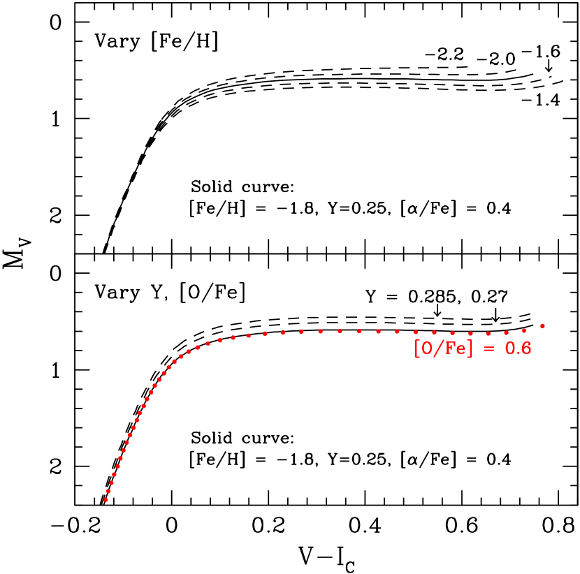
Figure 2.— Relative to the ZAHB represented by the solid curve, which was computed for indicated chemical abundances, the effects of varying [Fe/H] are shown in the top panel, whereas the effects of varying $Y$ and [O/Fe] are illustrated in the bottom panel.

When VandenBerg et al. (2013, hereafter VBLC13) determined the ages of more than 4 dozen GCs for which Sarajedini et al. (2007) had obtained Hubble Space Telescope (HST) photometry, they adopted $E(B-V)$ values from the Schlegel et al. (1998) dust maps and found that the morphologies of the blue HBs in clusters that possess them were reproduced exceedingly well by ZAHB models. Importantly, the distance moduli implied by the same ZAHB fits were in excellent agreement with those based on the RR Lyrae standard candle. Moreover, Paper I has shown that consistent interpretations of the data are obtained on both HST and Johnson-Cousins $BVI_{C}$ color planes when the same reddenings and distances are adopted. Since Schlegel et al. give $E(B-V)=0.135$ for M 55 and $E(B-V)=0.076$ for NGC 6362, we therefore anticipate being able to explain the CMDs and the properties of the RR Lyrae in these clusters on the assumption of reddenings that are reasonably close to these values.

As in Papers I and II, the pulsation periods are calculated using

$$\log\,P_{ab} ={}11.347+0.860\,\log(L/L_{\odot})-3.43\,\log{T_{\rm eff}}$$

$$-0.58\,\log({\cal{M}/\cal{M}_{\odot}})+0.024\,\log\,Z$$ (1)

and

$$\log\,P_{c} ={}11.167+0.822\,\log(L/L_{\odot})-3.40\,\log{T_{\rm eff}}$$

$$-0.56\,\log({\cal{M}/\cal{M}_{\odot}})+0.013\,\log\,Z.$$ (2)

These equations, which have been derived from sophisticated hydrodynamical models of RR Lyrae variables by Marconi et al. (2015), enable one to calculate the periods of the $ab$-type (fundamental mode) and $c$-type (first overtone) pulsators if the luminosity, effective temperature, and mass of each variable is found by interpolating with a grid of HB tracks that was computed for a metallicity $Z$ (i.e., the total mass-fraction abundance of all elements heavier than helium). As reported by Marconi et al., the uncertainties of the numerical coefficients and the constant terms in equations (1) and (2) are all quite small.

We now turn our attention to M 55, which bears considerable similarity to M 92 insofar as both have predominately blue HBs and relatively few RR Lyrae, though they have different metallicities by $\delta$[Fe/H] $\mathrel{\hbox{\raise 2.58334pt\hbox{$>$}\kern-7.3194pt\lower 2.15277pt\hbox{$\sim$}}}0.4$ dex.

3. M 55 (NGC 6809)

As is the case for a large fraction of the Galactic GCs, M 55 has been the subject of numerous studies over the years (e.g., Penny 1984; Briley et al. 1990; Mandushev et al. 1996; Vargas Álvarez & Sandquist 2007, hereafter VS07; Pancino et al. 2010). Most estimates of its metallicity have favored [Fe/H] $\approx-1.8$ (e.g., Zinn & West 1984, KI03, Kayser et al. 2008), but support can be found for both higher and lower values by $\sim\pm 0.15$ dex (see, e.g., Caldwell & Dickens 1988, Rutledge et al. 1997, Minniti et al. 1993, CBG09). Although $E(B-V)=0.08$ is listed for M 55 in the latest edition of the Harris (1996) catalog (see footnote 1), several studies have found that such a low value is problematic (see Schade et al. 1988, Mandushev et al. 1996, Kaluzny et al. 2014). Relatively high values ($\mathrel{\hbox{\raise 2.58334pt\hbox{$>$}\kern-7.3194pt\lower 2.15277pt\hbox{$\sim$}}}0.12$ mag) are permitted by the line-of-sight reddenings from dust maps (Schlegel et al. 1998, Schlafly & Finkbeiner 2011). Finally, the apparent distance moduli that have been derived for M 55, using a variety of methods, have tended to be in the range $13.9\mathrel{\hbox{\raise 2.58334pt\hbox{$<$}\kern-7.74998pt\lower 2.15277pt\hbox{$\sim$}}}(m-M)_{V}\mathrel{\hbox{\raise 2.58334pt\hbox{$<$}\kern-7.74998pt\lower 2.15277pt\hbox{$\sim$}}}14.15$ (Mandushev et al. 1996, Piotto & Zoccali 1999, VS07, VBLC13, Kaluzny et al. 2014).

For the present work, we decided to investigate the $B-V,\,V$ CMD for this cluster that was obtained by Kaluzny et al. (2010, hereafter KTKZ10), mainly because members of the same group (Olech et al. 1999) had previously determined intensity-averaged $V$ magnitudes ($\langle V\rangle$) and $\langle B\rangle-\langle V\rangle$ colors for the RR Lyrae in M 55. (Note that colors which are obtained from the difference of intensity-weighted mean magnitudes appear to be especially good approximations to the colors of equivalent static stars; see Bono et al. 1995.) As discussed by KTKZ10, their photometry was collected in a number of observing runs between May 1997 and June 2009 and they were calibrated to the standard Johnson-Cousins $BVRI_{C}$ system using transformations given by Stetson (2000). However, in contrast with our findings in the case of M 3, M 15, and M 92 (see Paper I), we were unable to achieve a fully consistent fit of our ZAHB models to these $BV$ observations and the HST $F606W,\,F814W$ photometry by Sarajedini et al. (2007) for the bluest HB stars in M 55. As reported by VBLC13 in their study of 55 of the GCs observed by Sarajedini et al., our ZAHB models generally provide very satisfactory fits to the morphologies of observed HBs on the assumption of well supported reddenings and distances. This led us to wonder if there may be small zero-point errors in the photometric data provided by KTKZ10.

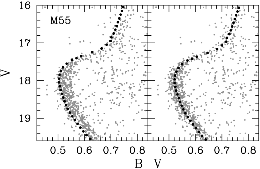
Figure 3.— Left-hand panel: comparison of the median fiducial sequence (black, filled circles) that represents the $B-V,\,V$ CMD of M 55 by Kaluzny et al. (2010) with the standard-field photometry (gray points) from P. Stetson’s archive (see the text for details and the relevant website address). Right-hand panel: similar to the left-hand panel, except that the sequence of black, filled circles has been adjusted by $\delta(B-V)=0.017$ mag and $\delta\,V=0.017$ mag prior to being plotted.

One way of checking into this possibility is to compare the CMD procured by KTKZ10 with the one that can be derived from the publicly available “Photometric Standard Fields” archive that was developed by Stetson (2000) and subsequently maintained by him. Since this database has been steadily evolving since its inception (see, e.g., Stetson 2005), one can anticipate that the latest calibrations of secondary cluster standards will differ to some extent from those reported by Stetson (2000). In fact, as shown in the left-hand panel of Figure 3, the $B-V,\,V$ diagram for M 55 from this archive does differ in small, but significant, ways from the KTKZ10 CMD, which is represented by the small black filled circles. (This fiducial sequence consists of the median points in 0.1 mag bins that were determined for the region of the CMD within $\sim\pm 2$ mag of the turnoff (TO). Because there are only about a half-dozen blue HB stars in Stetson’s archive, which show considerable scatter, any zero-point offsets that might be present are most readily seen by comparing the turnoff photometry from the two sources.) In order for the fiducial sequence to reproduce the archival data, it must be corrected by $\delta(B-V)=0.017$ mag and $\delta\,V\approx 0.017$ mag, resulting in the comparison between the two that is illustrated in the right-hand panel. (The color adjustment is more reliably determined and more important than the magnitude offset, which could be larger or smaller than our estimate by $\sim 0.03$ mag.)

Independent $BV$ photometry for the HB stars in M 55 by VS07 provides important confirmation of these offsets. This data set contains more HB stars in the vicinity of the knee, and somewhat larger scatter (see the upper panel of Figure 4) than the KTKZ10 CMD (lower panel). Nevertheless, the ZAHB that has been plotted, for [Fe/H] $=-1.80$, [$\alpha$/Fe] $=+0.4$, and $Y=0.25$, clearly provides a comparable fit to the observations from the two sources if the aforementioned adjustments are applied to the KTKZ10 CMD. (In this, and the next, plot, we have adopted the values of $E(B-V)$ and $(m-M)_{V}$ that are favored by our simulations of the cluster HB; see § 3.1. It turns out that nearly the same reddening, $E(B-V)=0.117$, is given by Schlafly & Finkbeiner (2011) from their recalibration of the Schlegel et al. (1998) dust maps.)

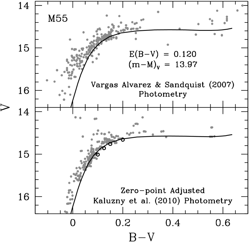
Figure 4.— Top panel: Comparison of HB photometry (gray points) for M 55 from VS07 with a ZAHB for [Fe/H] $=-1.80$, [$\alpha$/Fe] $=+0.4$, and $Y=0.25$. The models were shifted to the observed plane assuming $E(B-V)=0.12$ and $(m-M)_{V}=13.97$. Bottom panel: As in the top panel, except that the zero-point-adjusted photometry from Kaluzny et al. (2010) has been plotted (grey points). The four open circles indicate the red edge of the distribution of HB stars in the vicinity of the knee, based on the CMD published by Olech et al. (1999, see their Fig. 1). No zero-point corrections were applied to these data.

Thus, the offsets that were determined from the TO observations (see Fig. 3) are nearly the same as those needed to obtain consistency with the photometry of the HB by VS07. In addition, as shown by the small open circles in the bottom panel, the lower bound to the distribution of HB stars in the CMD obtained by Olech et al. (1999) matches its counterpart in the zero-point-corrected CMD of KTKZ10 quite well. (Differences in the calibration of the photometry, as described in the respective papers, likely explain why there are small offsets between them.) The open circles were obtained by producing a magnified version of Fig. 1 in the paper by Olech et al., drawing a smooth curve through the faintest stars in the vicinity of the knee of the blue HB, and then determining the $B-V,\,V$ co-ordinates at four locations on that curve. We conclude from this exercise that it is unnecessary to apply any adjustments to the values of $\langle V\rangle$ and $\langle B\rangle-\langle V\rangle$ that were determined by Olech et al. for the cluster RR Lyrae. (Although not shown, a comparison of the respective giant-branch loci supports this conclusion.)

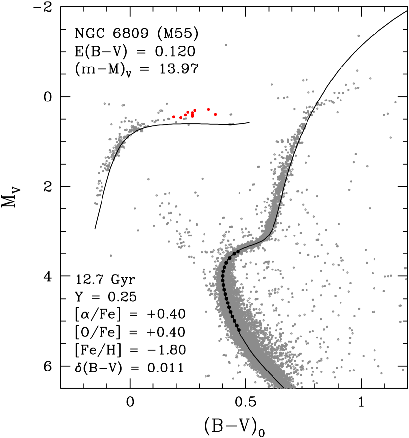
Figure 5.— Fit of a ZAHB and a 12.7 Gyr isochrone to the HB and turnoff (TO) observations of M 55, respectively, by Kaluzny et al. (2010), taking into account small zero-point adjustments amounting to $\delta(B-V)=0.017$ mag and $\delta\,V=0.017$ mag; see the text. (As noted by Kaluzny et al., the images of stars with $V<14.0$ mag were overexposed, which explains the odd morphology of the upper giant branch.) The indicated chemical abundances, reddening, and apparent distance modulus in the $V$ magnitude have been assumed. The small filled circles in the vicinity of the TO indicate the median fiducial sequence through the photometric data. In order to reproduce the observed TO color, the isochrone that provides the best simultaneous fit to the TO and the stars just beginning their subgiant evolution had to be corrected by only 0.011 mag (to the red). The small filled circles in red located just above the ZAHB represent cluster RR Lyrae stars, for which Olech et al. (1999) have derived intensity-weighted magnitudes and colors ($\langle V\rangle$ and $\langle B-V\rangle$).

Of the 15 RR Lyrae that were observed by Olech et al. (1999), two of them (V14 and V15) are suspected to be members of the Sagittarius dwarf galaxy, while three others (V9, V10, and V12) have irregular light curves that suggested (to them) the presence of non-radial oscillations. (These irregularities could alternatively be the manifestation of the Blazhko effect, as proposed for NGC 6362 variables that show similar anomalies by Smolec et al. 2017.) Of the remaining 10 RR Lyrae, V2, V4–V8, and V11 were found to be probable cluster members according to the recent proper motion study by Zloczewski et al. (2011). It is not known whether V1, V3, and V13 are members, and even though we have found irreconcilable differences between the predicted and observed periods of these stars (see below), there was no reason to exclude them from our sample of M 55 RR Lyrae at the outset of this work. In this investigation, we have therefore considered 10 variables, of which four are fundamental mode pulsators and the rest are first overtone pulsators. (To better approximate the colors of equivalent static stars, the small amplitude-dependent corrections to $\langle B\rangle-\langle V\rangle$ that were derived by Bono et al. (1995) for $ab$-type RR Lyrae have been taken into account. According to the latter, no such adjustments are needed for first overtone pulsators.)

On the assumption of what should be quite accurate estimates of $E(B-V)$ and $(m-M)_{V}$ (pending our analysis of the periods of the cluster RR Lyrae), we found that a 12.7 Gyr isochrone for the same chemical abundances ([Fe/H] $=-1.80$, [$\alpha$/Fe] $=+0.4$, and $Y=0.25$) does a good job of reproducing the TO observations. We checked, and found, that the models yielded essentially the same interpretation of HST observations for M 55 (Sarajedini et al. 2007), showing that there is rather good consistency between the two photometric data sets as well as the transformations from the $(\log\,{T_{\rm eff}},\,M_{\rm bol})$-diagram to the observed CMDs. (Because of its similarity with Fig. 5, a plot showing our fit of the same ZAHB and isochrones to the HST data has not been included in this paper.) The small offset between the giant-branch portion of the best-fit isochrone and the observed RGB could easily be caused by any one or more of the uncertainties that affect predicted temperatures and colors (some of which are listed in the last paragraph of this section).

As explained by VBLC13, only a narrow region of the CMD in the vicinity of the TO, where the shapes of isochrones are predicted to be nearly independent of, among other quantities, age and the mixing-length parameter, should be considered when determining the age corresponding to an adopted distance modulus. Using a well defined fiducial sequence to represent the turnoff observations facilitates the determination of the best-fit isochrone because it helps to ensure that each isochrone, in turn, is registered to exactly the same TO color when attempting to identify which one of them also reproduces the location of the stars just at the beginning of the SGB (those just brighter and redder than the TO). Only one isochrone can provide a simultaneous match of both of these features, for a given value of $(m-M)_{V}$, and it is the age of this isochrone that is the best estimate of the cluster age for the assumed chemical abundances. Even though a 12.7 Gyr isochrone clearly provides a very good fit to the median fiducial sequences in Figs. 5, it should be appreciated that an isochrone for a different age would provide an equally good fit had a larger or smaller distance modulus by the appropriate amount been assumed.

In order to match the TO photometry, it is generally necessary to correct the isochrone colors by a small amount that depends to some extent on the cluster and the filter passbands under consideration (see Papers I and II). Errors in the adopted color–${T_{\rm eff}}$ relations, the predicted temperatures (due, e.g., to inadequacies in the treatment of convection or the atmospheric boundary condition), the photometry, and/or the basic properties of a GC (reddening, distance, chemical composition) can easily explain such problems, but it is very difficult to determine which source of uncertainty is primarily responsible for them. However, it should be kept in mind that ad hoc corrections to the colors of isochrones have no significant impact on age determinations because the latter are derived from the magnitude difference between the ZAHB and the TO.

3.1. Simulations of the M 55 HB

As shown in Paper II, simulations of the HBs of observed CMDs, including the RR Lyrae components, are able to provide tight constraints on not only the cluster reddening and distance modulus but also the star-to-star variations in the initial helium abundance. Using the synthesis code introduced in that paper, we have generated synthetic HB distributions from newly computed grids of core He-burning tracks for [Fe/H] $=-1.80$, [$\alpha$/Fe] $=+0.4$, and several values of $Y$. These simulations have been compared with the observed distribution of the HB stars in M 55, on the assumption that its RR Lyrae have the colors and magnitudes of equivalent static stars derived from the values of $\langle B\rangle-\langle V\rangle$ and $\langle V\rangle$ that were derived by Olech et al. (1999), with the small adjustments given by Bono et al. (1995).

The best HB fit corresponds to the maximum probability predicted by the Kolmogorov-Smirnov (K-S) test (see Paper II) when we attempt to reproduce the observed distributions of the HB stars in both color and magnitude simultaneously, while varying the parameters in our HB population synthesis tool. These parameters include the relative fractions $f_{i}$ of the HB stars with different initial masses ${\cal M}_{i}$ and He abundances $Y_{i}$ that are used to represent the multiple stellar populations residing in a given GC, the mean masses that are lost by the RGB stars of these populations $\Delta{\cal M}_{i}$, and their standard deviations $\sigma_{i}$ — as well as the GC distance modulus and reddening. (For this exercise, we have assumed that the magnitudes of the brightest, unsaturated stars in the KTKZ10 CMD have $\sigma_{\rm phot}\leq 0.003$ mag.)

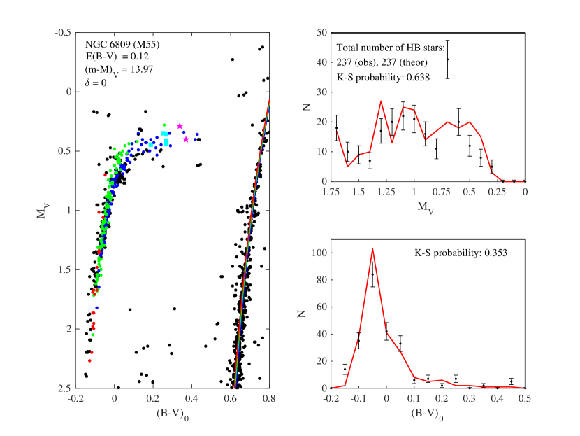
Figure 6.— Left-hand panel: overlay of a synthetic HB population of NGC 6809 (M 55) derived from evolutionary tracks for [Fe/H] $=-1.80$, [$\alpha$/Fe] $=0.4$, [O/Fe] $=0.4$, and $Y_{i}=0.25$, 0.265, and 0.28 (blue, green, and red filled circles, respectively) onto the observed CMD (black filled circles). RR Lyrae are represented by squares and star symbols. Right-hand panels: Comparisons of the predicted and observed numbers of HB stars (red loci and black dots with error bars, respectively) as a function of $M_{V}$ and $(B-V)_{0}$ color. The relatively high values of the K-S probability indicate that the simulated and observed distributions of stars are essentially equivalent.

The closest match that we were able to obtain between our synthetic HB populations and the observed HB in M 55 is shown in Figure 6 for the distance modulus and reddening that are indicated in the left-hand panel. Note that these estimates of $(m-M)_{V}$ and $E(B-V)$ differ by only 0.01 mag from the ZAHB-based determinations discussed in the previous section (see Figs. 4 and 5), which is well within photometric and fitting uncertainties. As in Paper II, the blue, green, and red filled circles in this panel represent the simulated HB populations with increasing helium abundances (specifically, $Y_{i}=0.25$, 0.265, and 0.28, respectively, in this case). The fractions of stars with these helium abundances and the corresponding values of the synthesis parameters are listed in Table 3. The squares and star symbols represent the RRc and RRab variables.

Table 3Fitted Parameters of M 55 from Simulations of its HB

Population ($i$)	$f_{i}$	$Y_{i}$	${\cal M}_{i}/{\cal M}_{\odot}$	$\Delta{\cal M}_{i}/{\cal M}_{\odot}$	$\sigma_{i}/{\cal M}_{\odot}$
$1$	$0.51$	$0.250$	$0.787$	$0.158$	$0.01$
$2$	$0.41$	$0.265$	$0.767$	$0.150$	$0.01$
$3$	$0.08$	$0.280$	$0.745$	$0.162$	$0.01$

Loci of the same colors that are superimposed on the cluster giants represent evolutionary tracks for 0.787, 0.767, and $0.745{\cal M_{\odot}}$, which are the adopted initial masses for the same three helium abundances, in the direction of increasing $Y_{i}$, for which the predicted age at the RGB tip is approximately 12.8 Gyr. These tracks provide a somewhat better fit to the giant branch than the isochrones that are plotted in the previous figure, in part because of small differences in the treatment of the surface boundary condition in the MESA and Victoria codes (as already noted in § 2), but also because the isochrones in Fig. 5 had been adjusted to the red by $\delta(B-V)=0.011$ mag in order to match the observed TO color.

The observational data in the right-hand panels are shown with Poisson error bars. The outlying point in the upper panel corresponds to a group of observed HB stars with $M_{V}\approx 0.7$ mag that our models cannot fully explain because they spread below the ZAHB. The mean masses that are lost by the RGB stars in M 55 are estimated to be $\Delta{\cal M}_{i}\approx 0.157\,{\cal M}_{\odot}$ for ${\cal M}_{i}\approx 0.766\,{\cal M}_{\odot}$, which is just slightly less than the amount expected from the Reimers (1975) formula with the parameter $\eta_{\mathrm{R}}=0.45$ (see Fig. 5 in Paper II). According to our simulations of the reddest HB stars in M 55, most if not all of its RR Lyrae variables are expected to have $Y\approx 0.25$.

3.2. The Periods of the RR Lyrae in M 55

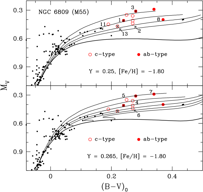
Figure 7.— Top panel: Fit of a ZAHB for the indicated chemical abundances and four post-ZAHB tracks (for $0.63\leq{\cal M}/{{\cal M}_{\odot}}\leq 0.66$, in the direction from left to right) to M 55 RR Lyrae (open and filled circles in red) and non-variable blue HB stars (small black filled circles), assuming $E(B-V)=0.120$ and $(m-M)_{V}=13.97$. The symbols for variables V1, V3, and V13 have been superimposed by crosses to indicate that there are large discrepancies between the predicted and observed periods (see the text). Bottom panel: As in the upper panel, except that the models assume $Y=0.265$ and the tracks are for masses $0.64\leq{\cal M}/{{\cal M}_{\odot}}\leq 0.69$ (in the direction from left to right).

Figure 7 shows the superposition of ZAHB loci and selected HB tracks from the grids discussed above for $Y=0.25$ (upper panel) and $Y=0.265$ (lower panel) onto the HB of M 55, assuming $E(B-V)=0.120$ and $(m-M)_{V}=13.97$. The filled and open circles (in red) represent the RRab and RRc variables, respectively. Once the luminosities, effective temperatures, and masses at these CMD locations have been determined using linear interpolations within, or minor linear extrapolations from, the tracks, the predicted periods of the RR Lyrae follow from equations (1) and (2). (The relevant values of $Z$ are $4.290\times 10^{-4}$, if $Y=0.25$, and $4.203\times 10^{-4}$, if $Y=0.265$.)

The differences between the predicted and observed periods (in days) of the 10 RR Lyrae are listed in Table 4, which also contains the results that are obtained if the same models are fitted to the observations, but a smaller value of $(m-M)_{V}$ by 0.05 mag, or a larger value by 0.03 mag is adopted. In both of the latter cases, the reddening was set (to the indicated values) so that the models always provide essentially the same fit to the blue HB stars with $M_{V}\mathrel{\hbox{\raise 2.58334pt\hbox{$>$}\kern-7.3194pt\lower 2.15277pt\hbox{$\sim$}}}0.8$. Note that a reduced distance modulus by 0.05 mag would imply an increased turnoff age by about 0.5 Gyr, and vice versa (see VBLC13, their Fig. 2). (Because the plots for the additional values of $E(B-V)$ and $(m-M)_{V}$ that we have considered in producing Table 4 are quite similar to those given in Figs. 5 and 7, we have opted not to include them in this paper. Indeed, there is sufficient ambiguity in the fits of ZAHB models and isochrones to the observed CMD of M 55 that they cannot be used to discriminate between the three cases considered in Table 4. However, it is clear from the tabulated results for the individual stars and the values of $\langle\delta P\rangle$ that the predicted periods are quite sensitive to the adopted cluster properties.)

Table 4Predicted minus Observed Periods

		$(m-M)_{V}=13.92$			$(m-M)_{V}=13.97$			$(m-M)_{V}=14.00$
		$E(B-V)=0.130$			$E(B-V)=0.120$			$E(B-V)=0.116$
Var.		$Y=0.25$	$Y=0.265$		$Y=0.25$	$Y=0.265$		$Y=0.25$	$Y=0.265$
$ab$-type
V1		$-0.128$*	$-0.139$*		$-0.089$*	$-0.098$*		$-0.070$*	$-0.078$*
V3		$-0.093$*	$-0.102$*		$-0.044$*	$-0.053$*		$-0.019$*	$-0.028$*
V7		$+0.023$*	$+0.011$*		$+0.085$*	$+0.071$*		$+0.117$*	$+0.101$*
V8		$-0.027$*	$-0.046$*		$+0.031$*	$+0.016$*		$+0.061$*	$+0.047$*
$c$-type
V2		$-0.019$*	$-0.031$*		$+0.015$*	$+0.006$*		$+0.031$*	$+0.023$*
V4		$+0.035$*	$+0.027$*		$+0.070$*	$+0.063$*		$+0.087$*	$+0.081$*
V5		$+0.020$*	$+0.014$*		$+0.053$*	$+0.047$*		$+0.069$*	$+0.064$*
V6		$+0.011$*	$+0.001$*		$+0.044$*	$+0.036$*		$+0.061$*	$+0.054$*
V11		$-0.010$*	$-0.018$*		$+0.015$*	$+0.008$*		$+0.027$*	$+0.021$*
V13		$-0.078$*	$-0.089$*		$-0.050$*	$-0.058$*		$-0.036$*	$-0.043$*
		$\langle\delta P\rangle=-0.004\pm 0.025$			$\langle\delta P\rangle=+0.035\pm 0.026$			$\langle\delta P\rangle=+0.056\pm 0.029$
Asterisks indicate the data used in calculating $\langle\delta P\rangle$ and the associated $1\,\sigma$ uncertainties.

As already mentioned, the measured periods of V1, V3, and V13 are difficult to explain insofar as they are much higher than the periods that are inferred from the CMD locations of these stars — as indicated by the large, negative values of $\delta P$ in Table 4. Because we do not have similar problems with the other RR Lyrae, crosses have been superimposed on the symbols representing these variables in Fig. 7 to indicate that they have been dropped from the remainder of our analysis. However, it is odd that V1 is bluer than most of the $c$-type variables ($\langle P_{c}\rangle\approx 0.38$ d), which is inconsistent with its high period (0.5800 d). V3 similarly seems anomalous in having quite a high period (0.6620 d) despite having nearly the same color, and hence ${T_{\rm eff}}$, as the reddest first overtone pulsators, which have shorter periods by $\sim 0.26$ d. (V3 is more luminous, but the luminosity difference is far too small to explain such a large discrepancy.) Finally, the similarity of the periods of V13 and V2, which have similar luminosities, is at odds with the significant difference in their colors (and presumably their temperatures). It goes without saying that further work is needed to resolve such apparent inconsistencies, which may be the manifestation of deficiencies in our understanding of pulsation physics, though we suspect that they are most likely due to errors in the derived mean properties if, indeed, V1, V3, and V13 are cluster members. (The periods of these stars cannot be the problem since they are determined to very high accuracy and precision from the light curves.)

Table 4 indicates that our models provide the best fits to the periods of the other RR Lyrae if M 55 has $(m-M)_{V}\approx 13.92$ (and $E(B-V)\approx 0.130$). (In all three cases that are tabulated, asterisks have been attached to the smallest $\delta P$ values.) A modulus as high as $(m-M)_{V}=14.00$ appears to be ruled out, given that the $\delta P$ values for most of the variables are unacceptably high for any $Y\leq 0.265$; as indicated at the bottom of the table, $\langle P\rangle=0.056\pm 0.029$ if all of them have $Y=0.265$. Even higher $Y$ is unlikely because the tracks for many of the variables would then have long blue loops, and the predicted ZAHB locations of many of the variables would be inside the instability strip. Since there are no RR Lyrae at such faint luminosities, it is much more credible that they originated from initial structures on the blue side of the instability strip where nearly all of the non-variable HB stars are found. Interestingly, if $(m-M)_{V}\approx 13.92$, the models for $Y=0.25$ predict periods that are closer to the observed periods of V2, V8, and V11 than those for $Y=0.265$, whereas the higher $Y$ models are favored in the case of V4–V7. However, such results are no more than suggestive because a change in $Y$ mainly affects the predicted mass at a given CMD location, which has a relatively minor impact on the pulsation period (see equations 1 and 2). According to the results presented in Table 4, an increase in the helium abundance by $\delta Y=0.015$ implies a reduced period by only $\sim 0.005$–0.015 days (if the temperature and luminosity are fixed).

Previous studies (VBLC13, Papers I and II) have not found any indications of substantial errors in the temperatures of our models for the HB phase, as they are able to reproduce the detailed morphologies of observed HBs over wide ranges in color and luminosity very well. (The same can be said of stellar models applicable to the TO and upper MS stars in GCs and in the field; see Brasseur et al. (2010) and VandenBerg et al. (2010, 2014a,b), who show that the model and IRFM ${T_{\rm eff}}$ scales are very similar and that isochrones generally provide quite consistent interpretations of observations on many different color-magnitude planes.) The predicted temperatures for warmer stars, such as those found in the instability strip and along the blue HB, should be particularly robust because surface convection zones are very thin or absent in them. Lacking any compelling evidence to the contrary, we are inclined to believe that the model ${T_{\rm eff}}$ scale is accurate to within $\sim\pm 80$ K ($1\,\sigma$), which is comparable to the uncertainties associated with empirical IRFM-based temperatures (e.g., see CRMBA).

For a typical RR Lyrae variable with ${T_{\rm eff}}=6750$ K ($\log{T_{\rm eff}}=3.83$), an error of $\pm 80$ K in its temperature would translate to an error in $\log P$ amounting to $\pm 0.017$ (see equations 1 and 2), which corresponds to $\delta P=0.016$ d if the star’s pulsation period is 0.400 d, or 0.024 d if $P=0.600$ d. Our HB tracks are based on up-to-date physics (see Paper I), including a treatment of mixing at the boundary of a convective He-burning core that is supported by asteroseismic studies of field HB stars (see Constantino et al. 2015, and references therein); consequently, they should provide especially realistic predictions of the paths that HB stars follow on the H-R diagram. In any case, errors in $\log(L/L_{\odot})$ (as well as in $\log({\cal M}/{{\cal M}_{\odot}})$ and $Z$) have significantly smaller effects on the predicted periods of RR Lyrae than errors in $\log{T_{\rm eff}}$. Based on these considerations, we expect that our models should be able to reproduce measured periods to within $\sim 0.03$ d. (This should be quite a realistic estimate since we have shown in Paper I that both the slope and the zero-point of the best available empirical $M_{V}$ vs. [Fe/H] relation for RR Lyrae stars is well reproduced by our models. This issue is revisited in § 5.)

Additional fits of our models to the HB of M 55 (not shown) indicate that the cluster must have $(m-M)_{V}\mathrel{\hbox{\raise 2.58334pt\hbox{$>$}\kern-7.3194pt\lower 2.15277pt\hbox{$\sim$}}}13.88$ in order to provide an acceptable interpretation of both the pulsational properties of the cluster RR Lyrae and the non-variable HB stars just blueward of the instability strip. Otherwise, the latter would lie fainter than the ZAHB and we would obtain $\langle\delta P\rangle<-0.03$ d for the variable stars. Even shorter distances would run into the aditional difficulties of requiring $E(B-V)>0.140$, for which there is no observational support, and the predicted TO age would be similar to, or exceed, the age of the universe ($\approx 13.8$ Gyr; Planck Collaboration 2015, Bennett et al. 2013). As a result of these considerations, we conclude that M 55 has $(m-M)_{V}=13.93\pm 0.05$. (This assumes, of course, that our evolutionary computations for the HB phase, and equations (1) and (2), accurately predict the properties of real stars in the core He-burning phase.) Due to the reduced distance modulus, the age derived previously ($\approx 12.7$ Gyr, see Fig. 5) rises to $\approx 13.1$ Gyr.

The apparent distance modulus that is derived in this way cannot be very dependent on the adopted metallicity because almost the same reddening is required to fit the blue HB stars just below the knee (this will be true even if the adopted [Fe/H] value is changed by as much as 0.3–0.4 dex; recall Fig. 2), and consequently, the temperatures that are derived for the RR Lyrae will be very similar. Hence, if models for different [Fe/H] values (within some reasonable range, say 0.25 dex) are to predict close to the measured periods, the luminosities of the variable stars cannot have much of a dependence on metallicity either. (Changing only the $M_{V}$ values of the RR Lyrae by, e.g., $-0.04$ mag, which is approximately the vertical shift of a ZAHB for [Fe/H] $=-2.0$ relative to one for [Fe/H] $=-1.8$, at the color of the instability strip, would alter the predicted periods by $\delta\log P\approx 0.014$, or $\delta P\approx 0.019$ d if $P=0.600$ d.) Some differences in the predicted masses and in the value of $Z$ corresponding to the adopted [Fe/H] value can be expected, but pulsation periods have considerably less sensitivity to these quantities than to $\log(L/L_{\odot})$ or $\log{T_{\rm eff}}$ (see equations 1 and 2).

While the uncertainties associated with the distance moduli as derived from our HB simulations, on the one hand, and from the RR Lyrae, on the other, overlap one another if [Fe/H] $\approx-1.8$, only marginal consistency would have been obtained had we adopted [Fe/H] $=-2.0$. As noted in the previous paragraph, fits of HB models for the lower metallicity to the photometric observations would yield $(m-M)_{V}\approx 14.01$, which is 0.08–0.09 mag larger than the distance modulus at which the predicted mean period of the RR Lyrae, $\langle P\rangle$, would be in good agreement with the observed value. Since this difference is approximately double that which is obtained if M 55 has [Fe/H] $=-1.8$, the RR Lyrae indicate a clear preference for [Fe/H] $\mathrel{\hbox{\raise 2.58334pt\hbox{$>$}\kern-7.3194pt\lower 2.15277pt\hbox{$\sim$}}}-1.8$ over a lower metallicity. We will now consider the additional constraint that is provided by a member binary star with well determined properties.

3.3. The Eclipsing Binary V54 in M 55

Having derived the distance modulus of M 55 to within $\sim\pm 0.05$ mag ($1\,\sigma$) from its RR Lyrae and non-variable HB stars, assuming that our stellar models for the core He-burning phase are reliable, we can now use the properties of the detached, eclipsing binary in this cluster, V54, to constrain the effective temperatures and the chemical composition of its components. For this part of the analysis, we need only those fundamental properties of V54 that are listed in Table 5, which have been taken from the study by Kaluzny et al. (2014). From the measured $V$ magnitudes and their uncertainties, it follows that the primary and secondary components of the binary have $M_{V}=4.47\pm 0.06$ and $7.05\pm 0.07$, respectively, if the apparent distance modulus of the cluster is $(m-M)_{V}=13.93\pm 0.05$.

Table 5Basic Properties of V54

Property	Primary	Secondary
Mass ($\cal M_{\odot}$)	$0.726\pm 0.015$	$0.555\pm 0.008$
Radius ($R_{\odot}$)	$1.006\pm 0.009$	$0.528\pm 0.005$
$B$ magnitude	$18.93\pm 0.01\phantom{0}$	$21.87\pm 0.03\phantom{0}$
$V$ magnitude	$18.40\pm 0.01\phantom{0}$	$20.98\pm 0.02\phantom{0}$

The extinction, $A_{V}$, is not needed to compute these $M_{V}$ values because the absolute magnitude scale was set by our HB models, though the apparent modulus that was derived does depend to some extent (see Table 4) on the adopted reddening. To convert the $M_{V}$ values to absolute bolometric magnitudes, it is necessary to know the temperatures of the components, which can be derived from the dereddened $B-V$ colors. However, the bolometric corrections in the $V$ band ($BC_{V}$) that apply to metal-poor stars located near the turnoffs of GCs are very weak functions of ${T_{\rm eff}}$, so it does not matter if the temperatures that are assumed for this part of the analysis are not accurate. As shown in Figure 8, which considers metallicities in the range $-2.0\leq$ [Fe/H] $\leq-1.6$, the $BC_{V}$ values of upper MS and TO stars vary, at a fixed value of $\log\,g$, by only $\sim 0.03$ mag over a 400 K range in ${T_{\rm eff}}$. (These results were obtained from the transformations provided by Casagrande & VandenBerg (2014), who computed $BC$s based on MARCS model atmospheres (Gustafsson et al. 2008) for many filter passbands over wide ranges in [Fe/H], [$\alpha$/Fe], $\log\,g$, and ${T_{\rm eff}}$.)

Figure 8.— The ${T_{\rm eff}}$ dependence of the bolometric corrections in the $V$ band for stars with [Fe/H] $=-1.6$ and $-2.0$ assuming, in each case, $\log\,g=4.0$ and 4.5 (as indicated). Turnoff stars in M 55 are predicted to have temperatures near 6300 K.

In any case, it is easy to obtain consistency between the temperatures that are derived from the luminosities and radii of the components of V54 and those assumed in the determination of the $BC_{V}$ values simply by iterating between the two. To be more explicit: we adopted initial values of ${T_{\rm eff}}$ that were calculated from the IRFM-based $(B-V)_{0}$–${T_{\rm eff}}$–[Fe/H] relation of CRMBA (see their Table 4), determined the corresponding values of $BC_{V}$ from the transformation tables provided by Casagrande & VandenBerg (2014), converted the resultant $M_{\rm bol}$ values to $\log\,(L/L_{\odot})$, and then calculated the temperatures of the binary from those luminosities and the measured radii. These ${T_{\rm eff}}$ values could then be used to recalculate the bolometric corrections, etc. After 4 iterations of this procedure, the input and output temperatures were the same, resulting in ${T_{\rm eff}}=6347\pm 116$ K and $5009\pm 104$ K, in turn, for the primary and secondary of V54. (The error bars were calculated from the $1\,\sigma$ uncertainties in the luminosities and radii.) These estimates compare very well with the values of ${T_{\rm eff}}=6361$ K and 5050 K, respectively, that are obtained from the CRMBA color-temperature-metallicity relation. Worth emphasizing is that our temperature determinations are independent of those inferred from spectra (e.g., the fitting of Balmer line profiles) or from the application of the IRFM.

As shown in Figure 9, the isochrones that provide the best fits to the observed CMD of M 55, on the assumption of the various chemical abundances that are specified in the lower left-hand corner of the upper panel, provide an excellent fit to the binary components on both the mass–radius plane and the $(\log{T_{\rm eff}},\,M_{V})$-diagram. Recall that the isochrone for [Fe/H] $=-1.80$ [$\alpha$/Fe] $=+0.4$, and $Y=0.25$ has an age of 13.1 Gyr. This rises to $\approx 14.0$ Gyr if the cluster turnoff is fitted by an isochrone for [Fe/H] $=-2.0$, assuming the same values of [$\alpha$/Fe] and $Y$. For the higher metallicity case, a 13.1 Gyr isochrone with $Y=0.27$ has also been plotted (the dashed curve) to illustrate the impact of varying this parameter. (M 55 probably has stars with even higher helium abundances given that such stars are expected to produce the bluest HB stars; see the discussion in Paper II of the especially long blue HB tail in M 13. In principle, this should be taken into account when fitting isochrones to the CMD of M 55, but this would cause only a minor perturbation to the derived age.)

The effect of increasing the oxygen abundance by 0.2 dex is shown by the dotted curve (in red). In this 12.6 Gyr isochrone, which provides as good a fit to the TO photometry as the other isochrones (on the assumption of the same distance modulus), the abundances of all of the other elements are the same as those assumed in the solid curve. The large red filled circle shows where a model for the same mass as the primary of V54 sits on the dotted isochrone in the two panels of Fig. 9.

While the various isochrones are nearly coincident on the $\log{T_{\rm eff}}$–$M_{V}$ plane, they are quite well separated on the mass–radius diagram, which provides a much better discriminant of the assumed chemical abundances. Unfortunately, even though the mass of the primary is known to within 2.1% (see Table 5), this uncertainty is still too large to place really tight constraints on $Y$. If M 55 has [Fe/H] $=-1.80$, [$\alpha$/Fe] $=0.4$, $(m-M)_{V}=13.93$, and an age of $\approx 13.1$ Gyr, the predicted masses for any helium abundance in the range $0.25\mathrel{\hbox{\raise 2.58334pt\hbox{$<$}\kern-7.74998pt\lower 2.15277pt\hbox{$\sim$}}}Y\mathrel{\hbox{\raise 2.58334pt\hbox{$<$}\kern-7.74998pt\lower 2.15277pt\hbox{$\sim$}}}0.28$ are consistent with the measured mass of the primary to within its $1\,\sigma$ error bar. The upper panel of Fig. 9 also indicates a preference for [O/Fe] $\leq 0.4$ if [Fe/H] $=-1.80$, though isochrones for a higher oxygen abundance by as much as $\sim 0.3$ dex (estimated by extrapolating the separation between the solid and dotted curves at the observed radius and then applying the result to the dot-dashed curve) would satisfy the mass constraint if M 55 has [Fe/H] $\approx-2.00$. Indeed, a higher oxygen abundance would be needed in this case to avoid a conflict between the age of M 55 and the age of the universe. Thus, [Fe/H] $<-2.0$ can be ruled out if M 55 has [O/Fe] $\mathrel{\hbox{\raise 2.58334pt\hbox{$<$}\kern-7.74998pt\lower 2.15277pt\hbox{$\sim$}}}0.4$. Models for [Fe/H] $>-1.80$ could be accommodated if they have [O/Fe] $<0.4$, which would, however, increase the predicted age at a given value of $(m-M)_{V}$. Based on these considerations, it would appear that M 55 has an age between $\approx 13.0$ Gyr and 13.8 Gyr, where the upper limit is set by the age of the universe.

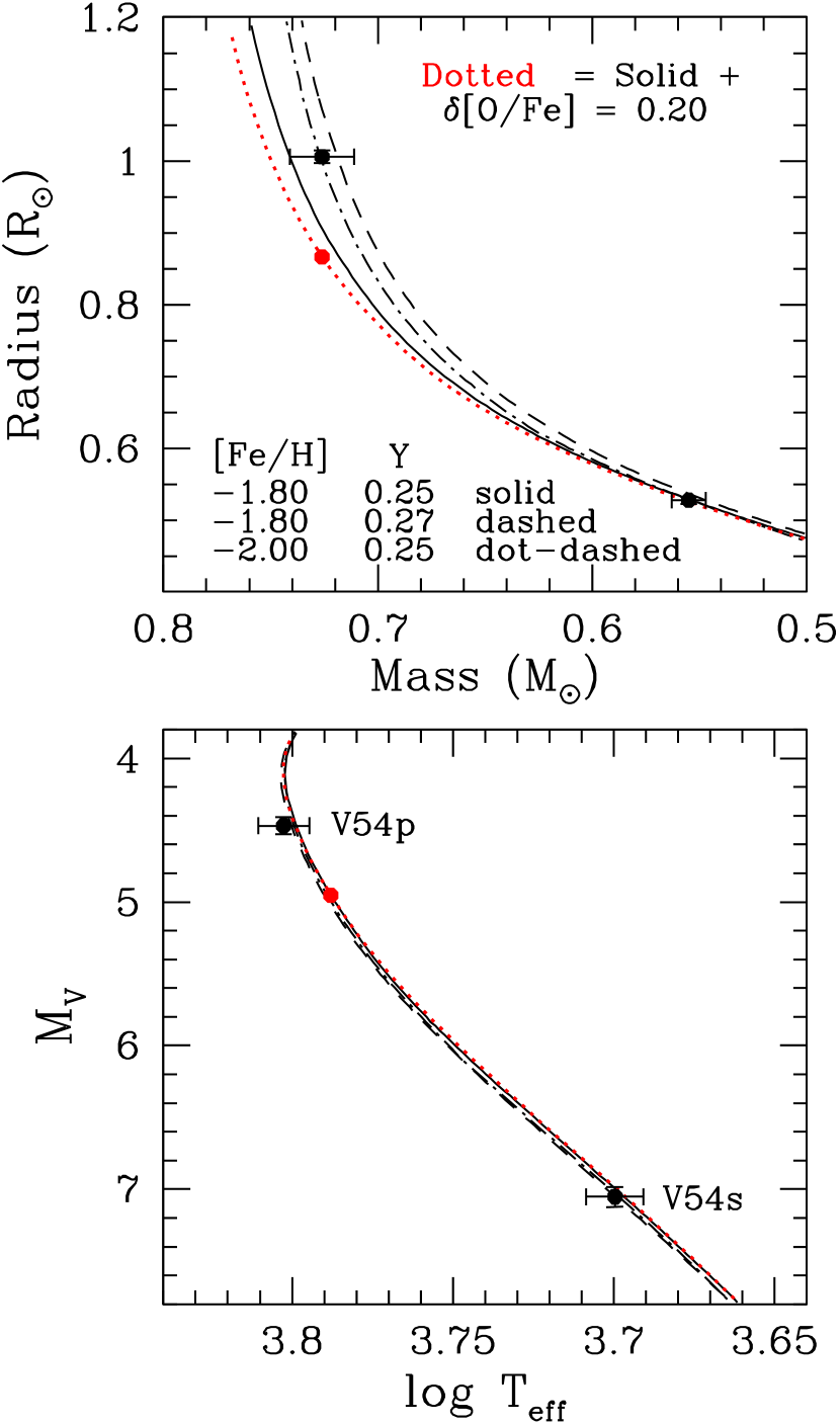
Figure 9.— Top panel: Comparison of the measured masses and radii of the components of V54 with the mass-radius relations predicted by isochrones for the indicated chemical abundances that provide the best fits to the turnoff photometry of M 55 (see the text). The large filled circle in red indicates the location of a stellar model along the dotted red isochrone that has the same mass as the primary of V54. Bottom panel: as in the top panel, except that the comparisons are made on the ($\log{T_{\rm eff}},\,M_{V}$)-diagram.

However, all of these inferences assume that V54 has $Y\approx 0.25$. Indeed, some of the stars in M 55 probably do have such helium abundances, but others are likely to have higher $Y$. This is suggested by our analysis of the cluster RR Lyrae, but more importantly, it is becoming clear that a spread in $Y$ is a common characteristic of GCs (see, e.g., Piotto et al. 2007; Milone et al. 2012, ; Nardiello et al. 2015, and our examination of both the variable and non-variable stars in M 3, M 13, and 47 Tuc that were presented in Paper II). Hence, it is easily possible that V54 is a member of a helium-enhanced population in M 55, in which case, models for [Fe/H] values as high as $\sim-1.6$, or those for, e.g., [Fe/H] $=-1.8$ and [O/Fe] $=0.6$, could satisfy the binary constraint if $Y\mathrel{\hbox{\raise 2.58334pt\hbox{$<$}\kern-7.74998pt\lower 2.15277pt\hbox{$\sim$}}}0.28$ (an estimate based on the results that are shown in the upper panel of Fig. 9). Since [O/Fe] $=0.6$ (i.e., an enhancement of 0.2 dex above the amount implied by [$\alpha$/Fe] $=0.4$) is a viable possibility, the absolute age of M 55 could be anywhere in the range from $\sim 12.6$ to 13.8 Gyr.

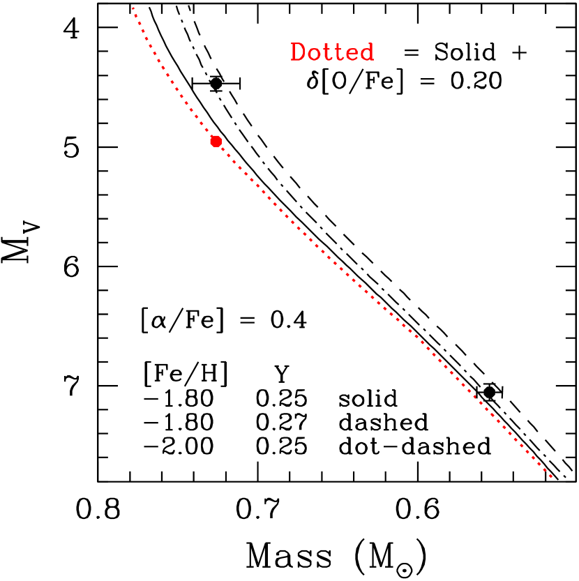
Figure 10.— As in the previous figure, except that the comparisons are made on the mass–$M_{V}$ diagram.

The mass–$M_{V}$ diagram, which is given in Figure 10, looks qualitatively very similar to the mass–radius diagram, and its implications for the cluster properties are clearly nearly the same as those just described. The main strength of stellar models has always been the prediction of the luminosities of stars; consequently, Fig. 10 provides a much more compelling comparison between theory and observations than those shown in the previous figure, though our success in matching the radii and temperatures of the V54 components as well as their luminosities, is very encouraging. Even though we are unable to place very tight limits on the chemical abundances of M 55 from comparisons of predicted mass-luminosity relations with the properties of the binary V54, it is comforting that the results from what is effectively a stellar interiors approach are consistent with, while being independent of, spectroscopically derived abundances.

In view of the high age that we have found for M 55 on the assumption of $(m-M)_{V}=13.93$, a reduced distance modulus by more than $\sim 0.05$ mag is unlikely because the consequent cluster age would be within $\sim 0.5$ Gyr of the age of the universe even if M 55 has [O/Fe] $\approx 0.6$ (assuming $-1.8\mathrel{\hbox{\raise 2.58334pt\hbox{$<$}\kern-7.74998pt\lower 2.15277pt\hbox{$\sim$}}}$ [Fe/H] $\mathrel{\hbox{\raise 2.58334pt\hbox{$<$}\kern-7.74998pt\lower 2.15277pt\hbox{$\sim$}}}-2.0$). This provides an indirect argument that the periods of the cluster RR Lyrae that are inferred from our HB tracks cannot be less than the observed periods by more than 0.03 d. What are the consequences, then, of adopting a larger distance modulus by 0.05 mag (i.e., $(m-M)_{V}=13.98$), in which case the predicted RR Lyrae periods would be greater than the observed periods by $\sim 0.03$ d?

For one thing, an increased distance would make V54 intrinsically brighter and its components would also be hotter, since their temperatures are calculated directly from their radii and luminosities. If $(m-M)_{V}=13.98$, we obtain ${T_{\rm eff}}=6415$ K and 5051 K, in turn, for the primary and secondary components. These estimates are still within the $1\,\sigma$ error bars of the temperatures previously derived on the assumption of the shorter distance modulus and, importantly, they are comparable with, or higher than, the temperatures found from the application of the IRFM by CRMBA. Indeed, the binary in M 55 provides compelling support for a relatively warm ${T_{\rm eff}}$ scale at low metallicities, which is one of the main results of this investigation.

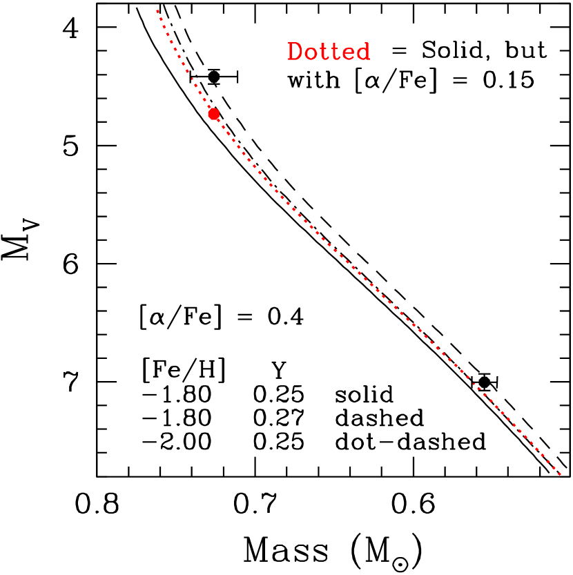
Figure 11.— As in the previous figure, except that a larger distance modulus by 0.05 mag has been assumed (specifically $(m-M)_{V}=13.98$), and younger isochrones by 0.5–0.6 Gyr have been plotted so as to be consistent with the increased distance. Note that, as a result of the change in $(m-M)_{V}$, the components of V54 will be instrinically more luminous and hotter.

Another consequence of adopting $(m-M)_{V}=13.98$ is that the turnoff age would be reduced by $\sim 0.5$–0.6 Gyr. Because younger ages imply higher masses at a given luminosity along the main sequence, the predicted mass–$M_{V}$ relations for the same chemical abundances considered in Fig. 10 would be shifted somewhat to the left of their locations therein. As shown in Figure 11, isochrones for $Y=0.25$ and [Fe/H] $\sim-1.8$ would be in poorer agreement with the properties of the binary than in Fig. 10 due to the net effect of this shift and the revised $M_{V}$ values of the binary. On the other hand, the models for $Y\mathrel{\hbox{\raise 2.58334pt\hbox{$>$}\kern-7.3194pt\lower 2.15277pt\hbox{$\sim$}}}0.26$ or for [Fe/H] $\sim-2.0$ and $Y\approx 0.25$ would still provide a satisfactory fit to the data to within $1\,\sigma$.

However, if V54 has [Fe/H] $=-1.80$ and $Y=0.25$, it is still possible to obtain consistency of the predicted and observed masses to within $1\,\sigma$ if a reduced O abundance is assumed. This is illustrated by the dotted isochrone (in red, from VandenBerg et al. 2014a), which assumes [$\alpha$/Fe] $=0.15$. (At low metallicities, the effects on isochrones of varying [$\alpha$/Fe] are due almost entirely to the associated changes in the O abundance; see VandenBerg et al. 2012.) To obtain a consistent fit to the turnoff photometry in this case, a higher age would have to be assumed, $\approx 13.3$ Gyr, which is not significantly different from the age that was derived on the assumption of $(m-M)_{V}=13.93$. On the other hand, a $\sim 12.6$ Gyr isochrone for [Fe/H] $=-1.80$ and [$\alpha$/Fe] $=0.4$ would provide a consistent interpretation of all of the observations (i.e., both the cluster CMD and the properties of V54) if the binary has $Y\approx 0.26$–0.28 (see Fig. 11). If the helium abundance is high enough, models for [O/Fe] $=0.6$ would also satisfy the binary constraint, and the resultant turnoff age would be close to 12.0 Gyr.

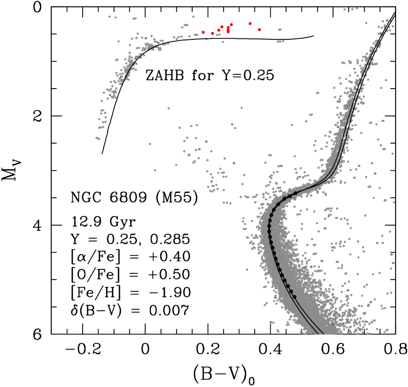
Figure 12.— Similar to Fig. 5, except that stellar models for different chemical abundances (as indicated) have been compared with the CMD of M 55. To match the cluster HB stars to a ZAHB for $Y=0.25$, compromise values of

$E(B-V)=0.125$ and $(m-M)_{V}=13.95$ have been assumed (see the text).

To summarize this section: our consideration of HB simulations and RR Lyrae periods suggests that M 55 has an apparent distance modulus in the range $14.93\mathrel{\hbox{\raise 2.58334pt\hbox{$<$}\kern-7.74998pt\lower 2.15277pt\hbox{$\sim$}}}(m-M)_{V}\mathrel{\hbox{\raise 2.58334pt\hbox{$<$}\kern-7.74998pt\lower 2.15277pt\hbox{$\sim$}}}14.97$ and [Fe/H] $=-1.85\pm 0.1$, which also satisfies the constraints provided by the eclipsing binary V54 to within the uncertainty of its helium abundance. Assuming that the cluster has [O/Fe] $=0.5\pm 0.1$, with [$m$/H] $=0.4$ for the other $\alpha$-elements, and that the faintest stars in the vicinity of the knee of the HB have $Y=0.25$, our best estimate of its age is $12.9\pm 0.8$ Gyr, where the error bar takes into account the effects of the distance and chemical abundance uncertainties (approximately $\pm 0.5$ Gyr and $\pm 0.3$ Gyr, respectively). The fit of a ZAHB and a 12.9 Gyr isochrone for these chemical abundances to the CMD of M 55 is shown in Figure 12. For illustrative purposes, an isochrone for the same age but for $Y=0.285$ has also been plotted; according to our HB simulations, few, if any, of the stars in M 55 have higher helium abundances.

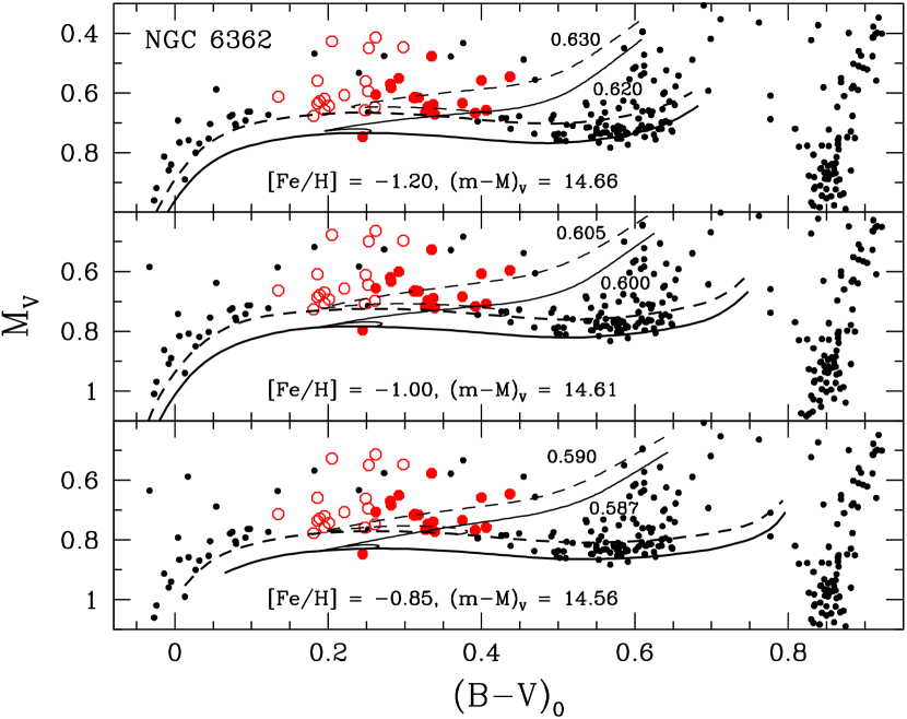
Figure 13.— Fits of ZAHB loci for $Y=0.25$ (thick solid curves) and $Y=0.265$ or 0.270 (thick dashed curves in the bottom or the top two panels, respectively) for the indicated [Fe/H] values and apparent distance moduli to the non-variable HB stars (small black filled circles) and the RR Lyrae in NGC 6263. The $ab$- and $c$-type variables have been plotted, in turn, as large filled and open circles in red. Cluster giants in the same magnitude range are located at $(B-V)_{0}\mathrel{\hbox{\raise 2.58334pt\hbox{$>$}\kern-7.3194pt\lower 2.15277pt\hbox{$\sim$}}}0.8$. In all three panels, $E(B-V)=0.070$ has been adopted (see the text for the justification of this choice). Two evolutionary tracks (for the indicated masses, in solar units) have also been plotted in each panel to illustrate their strong morphological dependence on $Y$.

4. NGC 6362

The basic properties of NGC 6362 appear to be relatively well determined. Most estimates of the foreground reddening fall in the range $0.07\mathrel{\hbox{\raise 2.58334pt\hbox{$<$}\kern-7.74998pt\lower 2.15277pt\hbox{$\sim$}}}E(B-V)\mathrel{\hbox{\raise 2.58334pt\hbox{$<$}\kern-7.74998pt\lower 2.15277pt\hbox{$\sim$}}}0.09$ (e.g., see Schlegel et al. 1998, Brocato et al. 1999, Olech et al. 2001, Schlafly & Finkbeiner 2011, and the 2010 edition of the catalogue by Harris 1996). Similar good consistency has been found for the cluster metallicity over the years, with the majority of studies finding [Fe/H] values between $-0.96$ (CG97) and $-1.15$ (KI03), including the investigations by, e.g., Zinn & West (1984), CBG09, Mucciarelli et al. (2016), and Massari et al. (2017). As first reported by Dalessandro et al. (2014), Mucciarelli et al. and Massari et al. have confirmed that, in common with most GCs, NGC 6362 contains multiple, chemically distinct stellar populations.

Because NGC 6362 has a well-populated red HB, along with a sufficient number of non-variable blue HB stars in the vicinity of the knee to provide a useful constraint on the reddening, fits of ZAHB models to the observed HB should be reasonably straightforward. However, it turns out that a single ZAHB locus cannot provide a satisfactory fit to the faintest HB stars across the entire color range that they occupy. The problem is that, as pointed out by Brocato et al. (1999), the HB of NGC 6362 has an odd HB morphology in that the faintest stars just to the blue of the instability strip are $\sim 0.1$ mag brighter than the faintest of the red HB stars; i.e., there is a significant downward tilt of the HB in the direction from blue to red. Although Brocato et al. suggested that variations in the bolometric corrections with [Fe/H] and ${T_{\rm eff}}$ may be responsible for this behavior, this speculation is not supported by our HB models. We believe, in fact, that the observed morphology is a manifestation of the multiple stellar populations phenomenon.

Figure 13 illustrates the fits of ZAHB loci for $Y=0.25$ (the thick solid curves) and either 0.27 (the thick dashed curves in the top and middle panels) or 0.265 (bottom panel) to the HB of NGC 6362 on the assumption of three different [Fe/H] values and distance moduli that have been derived by matching the faintest stars in the red HB to the ZAHB for $Y=0.25$ (as specified in each panel). Large open and filled circles, in red, indicate the locations of the RR Lyrae, for which Olech et al. (2001) provide intensity-weighted mean magnitudes and colors. (To better represent the colors of equivalent static stars, their $\langle B\rangle-\langle V\rangle$ values have been corrected by the amounts given by Bono et al. 1995.) As it turns out, the ZAHBs for the higher values of $Y$ provide good fits to the lower bound of the main distribution of these pulsators, as well as the non-variable stars on either side of the instability strip. To obtain nearly identical matches to the cluster stars in the color range $0.05\mathrel{\hbox{\raise 2.58334pt\hbox{$<$}\kern-7.74998pt\lower 2.15277pt\hbox{$\sim$}}}(B-V)_{0}\mathrel{\hbox{\raise 2.58334pt\hbox{$<$}\kern-7.74998pt\lower 2.15277pt\hbox{$\sim$}}}0.50$, it was necessary to adopt a slightly larger He enhancement in the top and middle panels.

These fits assumed $E(B-V)=0.070$, independently of the adopted metal abundance. Because the reddening has a direct impact on the ${T_{\rm eff}}$ scale of the RR Lyrae, we checked whether a consistent interpretation of HST photometry for NGC 6362 (Sarajedini et al. 2007) could be obtained on the assumption of the same reddening and distance moduli; and indeed, our ZAHB models for all three metallicities match the $F606W,\,F814W$ observations for the non-variable stars on both the blue and red sides of the instability strip just as well as in the three panels of Fig. 13. Since $E(B-V)=0.07$ is within 0.01 mag of dust map determinations (Schlegel et al. 1998, Schlafly & Finkbeiner 2011), this estimate appears to be particularly well supported. (Note that, because the redward extent of a ZAHB is quite a strong function of metallicity, it would not be possible to obtain a satisfactory fit of a ZAHB to the reddest HB stars if [Fe/H] $<-1.20$. Even [Fe/H] $=-1.20$ presents some difficulties in this regard as several of the cluster stars lie below the ZAHB for $Y=0.250$, though this discrepancy could be the consequence of small errors in the model colors.)

The distribution of the variable stars in NGC 6362 provides further evidence that they, along with bluer stars, have higher helium abundances than most of the reddest HB stars. (Since ZAHBs for $Y>0.25$ pass through the reddest stars, some of the latter could have higher $Y$.) In each panel, tracks for masses, in solar units, that are specified close to the ends of these evolutionary sequences, have been plotted that intersect the red edge of the main distribution of the $ab$-type RR Lyrae. The dashed tracks (for $Y\geq 0.265$) have long blue loops before the direction of the evolution turns back to the red, and curiously, they reproduce the locations of not only several of the fundamental mode pulsators near the ZAHB, but also some of them at higher luminosities. That is, these tracks follow the morphology of the red edge of the distribution of filled red circles remarkably well. Even if the computations for $Y=0.25$ did not suffer from the problem that the ZAHB is significantly fainter than all of the variable stars, except one, they predict blue loops that are too small to provide a comparable fit to the observations.

Interestingly, Mucciarelli et al. (2016) have reported that the [Na/Fe] distribution along the giant branch of NGC 6362 is broad and bimodal, and that $\sim 82$% of the red HB stars are Na-poor, from which they conclude that Na-rich stars on the RGB will populate the blue HB (though stars belonging to the latter were not included in their observing program). Thus, it would appear that there is a strong correlation of the Na and He abundances along the HB, which would not be at all surprising since H-burning nucleosynthesis at sufficiently high temperatures will tend to increase the abundance of sodium, thereby causing the O–Na anticorrelation that is a common characteristic of GCs. Based on the results shown in Fig. 13, we will initially assume that the RR Lyrae in NGC 6362 have $Y=0.265$ or 0.270, depending on the adopted metallicity, when we predict their periods from their CMD locations, though the brightest and bluest ones probably have even higher helium abundances.

4.1. The RR Lyrae Variables in NGC 6362

The binary mass-luminosity relation (to be discussed in § 4.4) appears to favor a relatively high metallicity for NGC 6362; consequently, we begin our analysis of the cluster RR Lyrae by fitting ZAHB models and HB tracks for $Y=0.265$ and [Fe/H] $=-0.85$ to the observations. According to the bottom panel of Fig. 13, most of the variable stars lie on or above this ZAHB, though it can be expected that some fraction of the brighter stars have somewhat greater helium abundances. Fortunately, the helium abundance uncertainty does not represent a serious concern for our results (see Papers I and II) because the effects of small changes in $Y$ on the mass, and hence the period, at a given CMD location are quite minor.

The faintest $ab$-type variable, V25, is considerably fainter than the others, and even though its CMD location suggests that it may have a helium abundance close to $Y=0.25$, the period predicted by models for this value of $Y$ is smaller than the observed period by $\sim 0.06$ days. Such a large discrepancy can hardly be due to a problem with our models because they are able to explain the periods of most of the cluster variables to within $\sim 0.02$ d (see below), including that of the bluest of the remaining fundamental mode pulsators (V3), which has nearly the same period and color as V25, despite being brighter by 0.14 mag. Such a large luminosity difference should give rise to a difference in period of nearly 0.05 d between V3 and V25. Because additional work is needed to understand its anomalous properties, V25 has been dropped from further consideration.

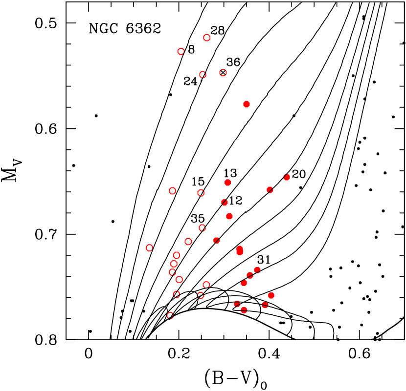
Figure 14.— Overlay of a ZAHB for $Y=0.265$, [$\alpha$/Fe] $=0.4$, and [Fe/H] $=-0.85$, along with HB tracks for 10 masses in the range $0.572\leq{\cal M}/{\cal M_{\odot}}\leq 0.600$ (in the direction from left to right), onto the HB of NGC 6362, assuming $E(B-V)=0.070$ and $(m-M)_{V}=13.56$. (The plot has been stretched in the vertical direction for the sake of clarity.) The open and filled circles, in red, indicate the CMD locations of the $c$-type and $ab$-type RR Lyrae, respectively. Variables are identified by their “V” numbers if the predicted and observed periods differ by $>0.030$ d. The symbol representing V36 has been superimposed by a cross to indicate that it has not been included in our analysis (see the text).

The same ZAHB (for $Y=0.265$) is shown in Figure 14 along with 9 evolutionary tracks for masses (in the direction from left to right) that range from 0.572 to 0.596 ${\cal M_{\odot}}$, in $0.003{\cal M_{\odot}}$ increments, and a tenth track for a mass of $0.600{\cal M_{\odot}}$. As these tracks follow blue loops that lie very close to the ZAHB, the plot has been stretched by a large amount in the vertical direction so that they can be easily distinguished. Since the tracks overlap one another near the ZAHB, there is obviously some ambiguity in determining the masses of the RR Lyrae in this region of the CMD. However, this uncertainty has only minor consequences for the predicted periods of these variables because the range in possible masses that could apply to a given star is small. Similarly, differences between the assumed and actual helium abundances at the level of $\Delta Y\mathrel{\hbox{\raise 2.58334pt\hbox{$<$}\kern-7.74998pt\lower 2.15277pt\hbox{$\sim$}}}0.01$ will not affect the interpolated masses and predicted periods of the RR Lyrae by very much. For the 5 variables in the overlap zone just above the ZAHB, masses were assigned (from the range of possible values implied by the superposition of the tracks onto the observed stars) that produced the best agreement between the predicted and observed periods.

Aside from the mass determination, it is straightforward to interpolate in, or extrapolate from, the tracks to obtain the luminosities and temperatures of the variable stars. Since the adopted chemical abundances correspond to $Z=3.729\times 10^{-3}$, equations (1) and (2) can be used to predict the periods of the RR Lyrae, and it turns out that the periods so obtained are generally in very good agreement with the observed periods. Only for the 10 variables that are identified in Fig. 14 did we find differences between the predicted and observed periods $>0.03$ days. The largest discrepancy was found for V36 ($>0.11$ d), which was dropped from our analysis because it clearly has anomalous properties. This leaves us with a sample of 17 RRab and 16 RRc stars.

Figure 15.— Comparison of the observed periods, in days, of the $ab$-type and $c$-type RR Lyrae in NGC 6362 with those determined from models for $Y=0.265$, [$\alpha$/Fe] $=0.4$, and [Fe/H] $=-0.85$. If the inferred temperatures of the variables are adjusted by the amounts specified in the lower right-hand corner, the mean values of $P_{ab}$ and $P_{c}$ from the models agree with the observed values of $\langle P_{ab}\rangle$ and $\langle P_{c}\rangle$, which are given in the top left-hand corner, to three decimal places. The differences between the predicted and observed periods have standard deviations amounting to $\sigma=0.026$ and 0.025 days (as indicated) for the RRab and RRc stars, respectively. Variable identification numbers are used to highlight the locations of the outliers in this plot (see the text for some discussion of these stars).

Figure 15 shows how well the observed periods of these RR Lyrae are reproduced by our models. From the differences between the observed periods and those calculated from equations (1) and (2), we obtain the mean offsets $\langle\Delta P_{ab}\rangle=-0.006\pm 0.026$ d and $\langle\Delta P_{c}\rangle=0.005\pm 0.025$ d, where the uncertainties represent the standard deviations of the mean. By applying the small zero-point adjustments that are given in the lower-right hand corner of the plot to the interpolated $\log{T_{\rm eff}}$ values of the variables, the observed values of $\langle P_{ab}\rangle$ and $\langle P_{c}\rangle$, which are specified in the top left-hand corner, are reproduced to three decimal places. (See Paper I for some discussion of the rationale behind the introduction of the $\delta{T_{\rm eff}}$ parameter.) That is, we obtain $\langle\Delta P_{ab}\rangle=0.000\pm 0.026$ d and $\langle\Delta P_{c}\rangle=0.000\pm 0.025$ d.

If all of the outliers that are identified in Figs. 14 and 15 had been removed from the sample, the resultant values of $\langle\Delta P_{ab}\rangle$ and $\langle\Delta P_{c}\rangle$ would have been $0.002\pm 0.012$ d and $0.000\pm 0.013$ d, respectively (without applying any adjustment to the derived temperatures). Clearly, there is very good consistency between the predicted and observed periods for the majority of the RR Lyrae in NGC 6362 if the cluster has [Fe/H] $\approx-0.85$. In fact, this was quite an unexpected result because Smolec et al. (2017) have reported that the light curves of 69% of the RRab stars and 19% of the RRc stars exhibit the Blazhko effect. It would seem that this is not a serious complication for most of these stars though this may provide at least a partial explanation of the seemingly anomalous periods (or CMD locations) of some of the outliers in Figs. 14 and 15, such as V12 and V13.

Before considering a lower metallicity, some additional remarks concerning Fig. 14 are warranted. In particular, the fairly sharp boundary between the fundamental and first-overtone pulsators seems contrary to expectations if the hysteresis effect (van Albada & Baker 1973) is a real phenomenon. If there was any significant delay in the transformation of an RRab star into an RRc star during the evolution from red to blue, and vice versa, the boundary between the $ab$- and $c$-type variables should be bluer at fainter values of $M_{V}$ than at higher luminosities, resulting in some overlap of the colors of the fundamental and first overtone pulsators. However, Fig. 14 gives the impression that the transition in the pulsation mode occurs at very nearly the same color regardless of the direction of evolution inside the instability strip; i.e., there does not appear to be a hysteresis effect. (This issue has been discussed much more thoroughly in connection with the RR Lyrae in M 5 by Arellano Ferro et al. 2016, see their section 4.2.)

Turning to the possibility that NGC 6362 has [Fe/H] $\approx-1.0$: a magnified version of the middle panel of Fig. 13 indicates that we would need to fit ZAHB models for a helium abundance slightly greater than $Y=0.270$ to the observations in order to match the faintest RR Lyrae. Rather than compute a new grid of models for the optimum helium abundance (estimated to be $Y=0.273$), we opted to shift the $Y=0.27$ grid for [Fe/H] $=-1.0$ by $\delta M_{bol}=-0.008$ mag so as to achieve the fit to the data that is shown in Fig. 16. The main consequence of this approximation is that the inferred masses of the variable stars will be too small by a few thousandths of a solar mass, but this will introduce only a small error ($\mathrel{\hbox{\raise 2.58334pt\hbox{$<$}\kern-7.74998pt\lower 2.15277pt\hbox{$\sim$}}}0.003$ d) in the predicted periods. Larger errors will certainly arise from the assumption of constant $Y$, as it seems likely that some of the variables will have appreciably higher helium abundances. Still, the increased distance modulus that is associated with a reduction in [Fe/H] from $-0.85$ to $-1.0$ will have a much larger effect on the predicted periods than those arising from star-to-star helium abundance variations.

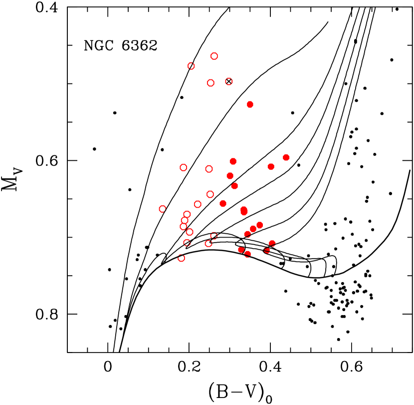
Figure 16.— Similar to Fig. 14, except that $(m-M)_{V}=14.61$ and $E(B-V)=0.070$ have been assumed, and the observations are compared with stellar models for [Fe/H] $=-1.00$. The HB tracks, in the direction from left to right, are for $0.580{\cal M_{\odot}}$, $0.590{\cal M_{\odot}}$, and $0.600\leq{\cal M}/{\cal M_{\odot}}\leq 0.620$, in $0.005{\cal M_{\odot}}$ increments. As explained in the text, ZAHB models for $Y\approx 0.273$ would provide a better match to the faintest RR Lyrae than those for $Y=0.270$. To provide a reasonable approximation to the former, the ZAHB and HB tracks for $Y=0.270$ have been adjusted by $\delta M_{\rm bol}=-0.008$ mag.

In fact, increasing the adopted value of $(m-M)_{V}$ by 0.05 mag results in larger periods by $\sim 0.02$ d, while the net effect on the periods of changes to the value of $Z$ and to the interpolated temperatures and masses is very much smaller. Thus, if the properties of the variables are obtained by interpolating in the models for [Fe/H] $=-1.0$ ($Z=2.626\times 10^{-3}$), we obtain $\langle\Delta P_{ab}\rangle=0.018\pm 0.029$ d and $\langle\Delta P_{c}\rangle=0.016\pm 0.027$ d for the mean differences between the predicted and observed periods of the 17 RRab and 16 RRc stars in our sample. It would be possible to reduce these offsets to 0.0 by, e.g., making an adjustment to the temperatures of the variables amounting to $\delta{T_{\rm eff}}=0.0040$ for the RRab pulsators and $\delta{T_{\rm eff}}=0.0065$ for the RRc stars — offsets that are within the $1\,\sigma$ uncertainties of the model ${T_{\rm eff}}$ scale.

Alternatively, an increased reddening by only 0.01 mag can accomplish almost the same thing. That is, if we were to adopt $E(B-V)=0.08$ for NGC 6362 and then compute the periods of its RR Lyrae from their interpolated properties, we would obtain $\langle\Delta P_{ab}\rangle=0.001\pm 0.028$ and $\langle\Delta P_{c}\rangle=0.009\pm 0.025$ days. Thus, even though the apparent distance modulus is virtually independent of $E(B-V)$, because it is based on a fit of ZAHB models to the reddest HB stars where the ZAHB is nearly horizontal, there is sufficient uncertainty in the reddening that, with a small adjustment to the adopted $E(B-V)$ value, it is possible to obtain satisfactory agreement between the predicted and observed periods over a fairly wide range in [Fe/H] (from, say, $\sim-0.8$ to $\sim-1.1$). Whether or not simulations of the entire HB population are able to place tighter constraints on the cluster metallicity is examined in the next section.

Table 6Fitted Parameters of NGC 6362 from Simulations of its HB

Population ($i$)	$f_{i}$	$Y_{i}$	${\cal M}_{i}/{\cal M}_{\odot}$	$\Delta{\cal M}_{i}/{\cal M}_{\odot}$	$\sigma_{i}/{\cal M}_{\odot}$
[Fe/H] $=-0.85$
$1$	$0.36$	$0.250$	$0.860$	$0.240$	$0.01$
$2$	$0.34$	$0.265$	$0.835$	$0.245$	$0.01$
$3$	$0.30$	$0.280$	$0.815$	$0.243$	$0.01$
[Fe/H] $=-1.00$
$1$	$0.45$	$0.250$	$0.837$	$0.195$	$0.01$
$2$	$0.45$	$0.265$	$0.813$	$0.212$	$0.01$
$3$	$0.10$	$0.280$	$0.790$	$0.208$	$0.01$

4.2. Simulations of the NGC 6362 HB

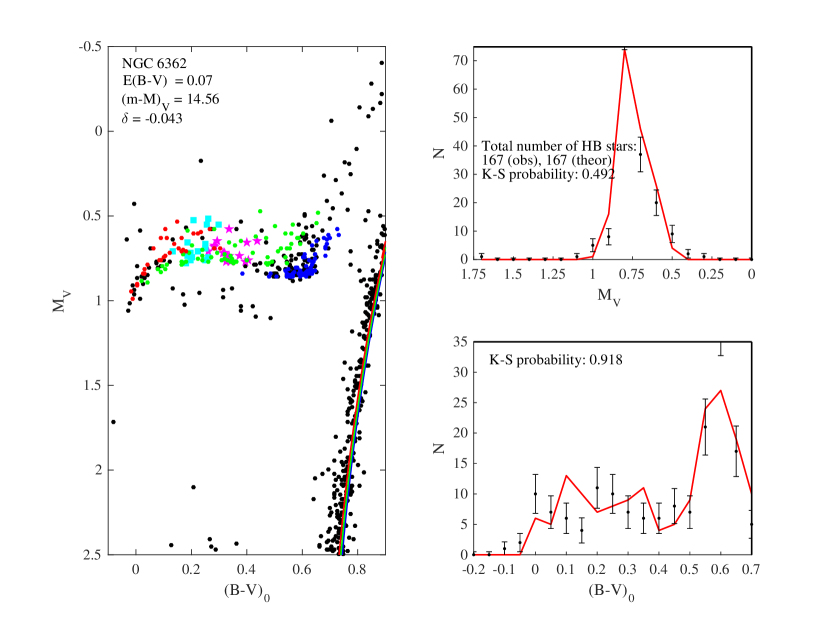
Figure 17.— As in Fig. 6, except that a synthetic HB for NGC 6362 has been generated from tracks for [Fe/H] $=-0.85$, [$\alpha$/Fe] $=0.4$, and $Y=0.25$, 0.265, and 0.28 (blue, green, and red filled circles, respectively. Superimposed on the cluster giants are evolutionary tracks for 0.86, 0.835, and $0.815{\cal M_{\odot}}$ for the same three values of $Y$, in turn; see the discussion of similar models in connection with Fig. 6.

Using the same procedures that were briefly summarized in § 3.1, we have generated synthetic HB populations applicable to NGC 6362 from evolutionary tracks for [Fe/H] $=-0.85$ and $-1.0$ assuming, in both cases, [$\alpha$/Fe] $=+0.4$ and $Y=0.25$, 0.265, and 0.28. (For these simulations, the photometric uncertainty was taken to be $\sigma_{\mathrm{phot}}\approx 0.005$ mag, as determined for the brightest stars in the sample of nearly 10,000 proper-motion selected members that were observed by Zloczewski et al. 2012.) With the fitting parameters set to the values listed in Table 6, the simulated HBs for metallicities that differ by 0.15 dex provide equally satisfactory fits to the observations, according to the calculated Kolmogorov-Smirnov probability. For instance, the best fit of our synthetic HB for [Fe/H] $=-0.85$ to the observed distribution of RR Lyrae stars from Olech et al. (2001) and non-variable stars from Zloczewski et al. is shown in Figure 17. If the simulations are based instead on the models for [Fe/H] $=-1.0$, the calculated K-S statistic for our best matches to the observed numbers of stars as functions of absolute magnitude and $(B-V)_{0}$ color are, in turn, 0.612 and 0.791 (i.e., just slightly higher and lower, respectively, than the values reported in Fig. 17).

However, in order to achieve this, stars with [Fe/H] $=-0.85$ would have to lose more mass along the RGB and a higher fraction of the stars in NGC 6362 would need to belong to the most helium-rich population (see Table 6). This is a possible problem, as a mean mass loss of $\sim 0.24\,{\cal M_{\odot}}$ is significantly higher than we have found for both more metal-poor and more metal-rich GCs that we have studied so far in this series of papers. Indeed, the predicted mass loss if [Fe/H] $=-1.0$ agrees very well with the estimate of $\Delta{\cal M}_{i}\approx 0.21\,{\cal M}_{\odot}$ that is obtained for a star with an initial mass ${\cal M}_{i}\approx 0.825\,{\cal M}_{\odot}$ and the adopted chemical abundances if $\eta_{\mathrm{R}}=0.45$ is assumed in Reimers’ mass-loss formula. (Recall our demonstration in Paper I that differences in $Y_{i}$ should not affect the Reimers mass-loss estimate.) This suggests that the metallicity of NGC 6362 may be closer to $-1.0$ than to $-0.85$.

The fits of theoretical distributions of HB stars to the observations are quite sensitive to variations in the fractions of their multiple populations $f_{i}$. For both NGC 6362 and M 55, a 5–10% change in the fractions of the first two populations, those for $Y_{1}=0.25$ and $Y_{2}=0.265$, results in a significant reduction of the K-S probabilities. In the case of NGC 6362, it is the K-S probability for the color fit that is the most sensitive to variations of $f_{1}$ at a fixed value of $f_{3}$. For instance, although our best HB fit on the assumption of [Fe/H] $=-1.0$ yielded $f_{1}=0.45$ and $f_{3}=0.10$ (see Table 6), comparatively good fits are also obtained for $f_{1}=0.50$ at both $f_{3}=0.10$ and $f_{3}=0.05$. However, larger variations of $f_{1}$ lead to significant reductions in the K-S probability for the color fit (by more than a factor of two, and increasing with the variation). A similar result is obtained if the adopted metallicity is [Fe/H] $=-0.85$. The HB fits are much more sensitive to variations in the RGB mass loss, for which changes of a few percent lead to significant reductions of the K-S probabilities.

In excellent agreement with the distance moduli that are obtained from fits of ZAHB models to the observed HB (see Figs. 13, 14, and 16), our simulations yield $(m-M)_{V}=14.56$ if [Fe/H] $=-0.85$ and $(m-M)_{V}=14.60$ if [Fe/H] $=-1.0$. For both of these determinations, the adopted reddening is $E(B-V)=0.07$. By comparison, in a paper that was submitted for publication concurrently with ours, Arellano Ferro et al. (2018) derived $E(B-V)=0.063\pm 0.024$, [Fe/H] $=-1.066\pm 0.126$, and $(m-M)_{V}=14.69\pm 0.08$ from new time-series CCD $VI$ photometry of the $ab$-type RR Lyrae (with very similar results for the RRc stars). To within the uncertainties, these results are fully consistent with our determinations.

4.3. The Age of NGC 6362

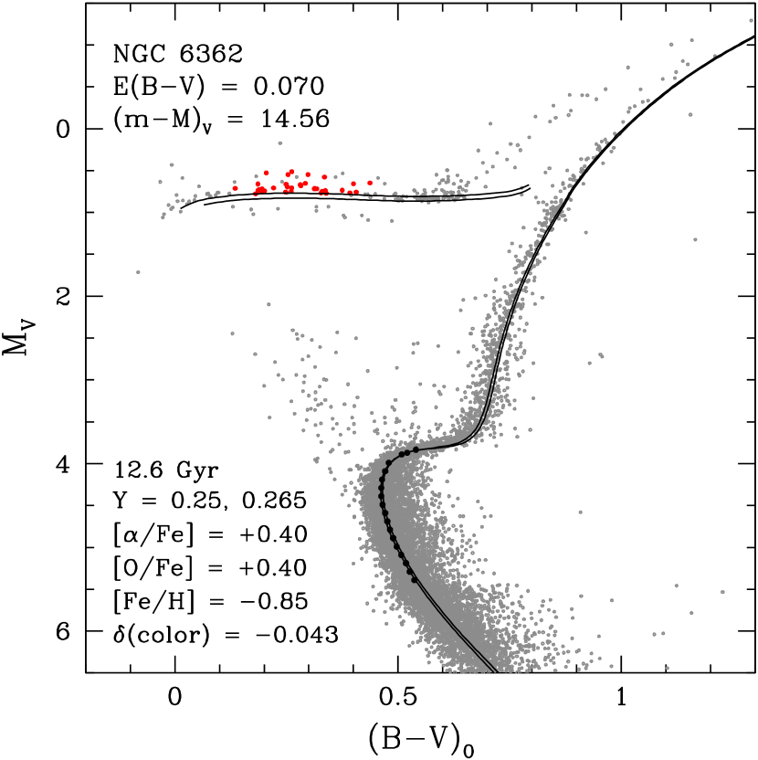
Figure 18.— Similar to Fig. 5, except that ZAHBs and 12.6 Gyr isochrones for the indicated helium and metal abundances have been fitted to the CMD of NGC 6362 (from Zloczewski et al. 2012), on the assumption of the reddening and apparent distance modulus that are specified in the top left-hand corner.

Since the binaries in NGC 6362 are comprised of stars that are located near the cluster turnoff, we need to identify which isochrones should be compared with their properties. The necessary next step in our analysis is therefore the determination of the age of NGC 6362 on the assumption of our best estimates of its reddening and distance modulus. As in the case of M 55 (see § 3), the median fiducial sequence for stars in the vicinity of the turnoff was derived in the usual way (see Paper II) so that the procedure used to select the best-fit isochrone involves very little, if any, subjective errors.

Figure 18 shows that 12.6 Gyr isochrones for [Fe/H] $=-0.85$, [$\alpha$/Fe] $=+0.4$, and $Y=0.25$, 0.265 provide very good fits to the turnoff of NGC 6362 if $E(B-V)=0.070$ and $(m-M)_{V}=14.56$ (as derived in the preceding sections). The relatively small change in $Y$ clearly has a much bigger impact on models for core He-burning stars than on those for the MS and RGB phases of evolution. Although Fig. 18 gives the impression that the observed subgiant branch is somewhat more steeply sloped than those of the isochrones, this may be the result of whatever is causing the predicted RGB to be offset slightly to the red of the cluster giants. For instance, if we forced the predicted giant branch to match the observed one by, among other possibilities, allowing for a small increase in the mixing-length parameter between the TO and the RGB or making suitable adjustments to the atmospheric boundary condition, the SGB slope discrepancy would no longer be apparent.

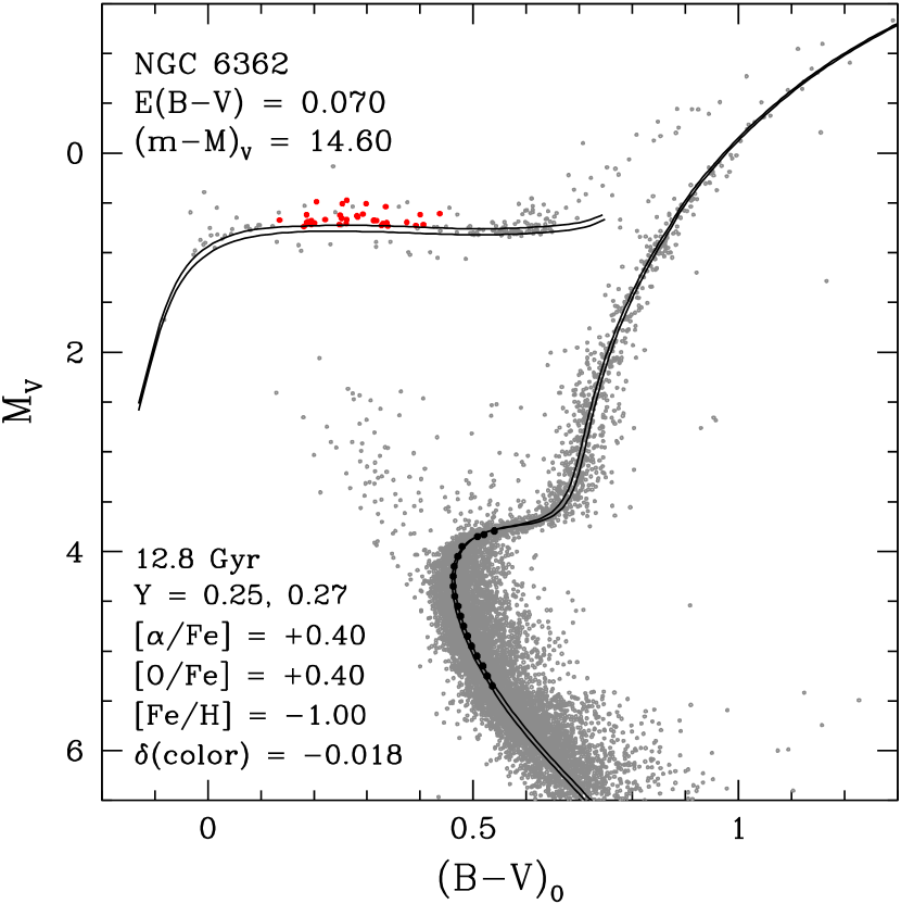
Figure 19.— As in the previous figure, except that models for [Fe/H] $=-1.0$ are compared with the observations.

On the other hand, a lower metallicity can accomplish the same thing. As shown in Figure 19, 12.8 Gyr isochrones for [Fe/H] $=-1.0$ provide a significantly improved fit to the cluster CMD. If a small zero-point adjustment is applied to the isochrone colors ($-0.018$ mag), the models reproduce the locations and the slopes of the MS, SGB, and RGB populations rather well. Even so, this is not a compelling argument in support of this possibility because there are so many factors, each with significant uncertainties, that impact the model ${T_{\rm eff}}$ and color scales. Because turnoff ages depend quite strongly on the total C$+$N$+$O abundance (VandenBerg et al. 2012), NGC 6362 could easily be several hundred Myr younger or older than the ages given in Figs. 18 and 19. For instance, if the cluster stars have [O/Fe] $=+0.6$, to be consistent with recent findings for field stars of similar metallicity (e.g., Zhao et al. 2016), the turnoff age would be $\approx 0.5$ Gyr less than that derived from models for [O/Fe] $=+0.4$ (assuming the same distance modulus and [$\alpha$/Fe] $=0.4$ for the abundances of the other $\alpha$-elements). However, because different C$+$N$+$O abundances will affect the mass-luminosity relation of the best-fit isochrone, we should be able to use the eclipsing binaries in NGC 6362 to discriminate between the possible metal abundance mixtures (at least in principle).

4.4. The Binaries V40 and V41 in NGC 6362

Table 7Basic Properties of V40 and V41

Property	Primary	Secondary
V40
Mass ($\cal M_{\odot}$)	$0.8337\pm 0.0063$	$0.7947\pm 0.0048$
Radius ($R_{\odot}$)	$1.3253\pm 0.0077$	$0.997\phantom{0}\pm 0.013\phantom{0}$
$V$ magnitude	$18.698\pm 0.020\phantom{0}$	$19.338\pm 0.027\phantom{0}$
$B-V$ color	$0.542\phantom{0}\pm 0.023\phantom{0}$	$0.556\phantom{0}\pm 0.034\phantom{0}$
V41
Mass ($\cal M_{\odot}$)	$0.8215\pm 0.0058$	$0.7280\pm 0.0047$
Radius ($R_{\odot}$)	$1.0739\pm 0.0048$	$0.7307\pm 0.0046$
$V$ magnitude	$19.089\pm 0.017\phantom{0}$	$20.274\pm 0.018\phantom{0}$
$B-V$ color	$0.550\phantom{0}\pm 0.018\phantom{0}$	$0.650\phantom{0}\pm 0.022\phantom{0}$

Kaluzny et al. (2015) determined the main properties of the detached, eclipsing binaries V40 and V41 in NGC 6362; their results for those quantities that are used in this investigation are listed in Table 7. Note that the masses of the binary components are known to within 0.76%, whereas the derived radii have uncertainties amounting to $<1.3$%. Using the same procedures that are described in detail in § 3.3, we can evaluate the luminosities of the components of V40 and V41, and then calculate their temperatures from the resultant luminosities and the tabulated radii. The same isochrones that were discussed in the previous section are compared with the binaries on the mass–$M_{V}$ and $\log\,{T_{\rm eff}}$–$M_{V}$ diagrams in Figure 20.

Figure 20.— Left-hand panels: superposition of the mass–$M_{V}$ relations predicted by the isochrones that were fitted to the CMD of NGC 6362 in Figs. 18 and 19 onto the derived masses and absolute $V$ magnitudes of the components of V40 and V41. The dot-dashed isochrones, which assumes [O/Fe] $=0.6$ and 0.4 dex enhancements of the other $\alpha$-elements, were computed for ages of 12.1 and 12.3 Gyr for the [Fe/H] $=-0.85$ and $-1.0$ cases, respectively. Right-hand panels: as in the left-hand panels, except that the comparisons are made on the $\log{T_{\rm eff}}$–$M_{V}$ plane.

Unfortunately, as already shown in our study of M 55 (see Figs. 10 and 11), mass–$M_{V}$ relations are much more dependent on the helium abundance than on [O/Fe]. An increase in $Y$ by only $\sim+0.0075$ (half of the separation between the solid and dashed loci in the upper left-hand panel of Fig. 20) causes a slightly larger increase in the mass at a given absolute magnitude than a $+0.2$ dex increase in [O/Fe] (the separation between the solid and dot-dashed curves). Since the helium contents of stars in NGC 6362 must vary by at least $\delta Y=0.015$–0.03 in order to explain the observed HB (in good agreement with the helium abundance variation derived by Gratton et al. 2010), V40 and V41 could be members of the population with $Y\approx 0.250$ or those with $Y\approx 0.265$–0.28 or any intermediate helium abundance. Taken at face value, the upper left-hand panel suggests that the binaries have $Y=0.25$ and [$\alpha$/Fe] $=0.4$ if they have [Fe/H] $\approx-0.85$, whereas the lower left-hand panel indicates a preference for the dot-dashed isochrone among those computed for [Fe/H] $=-1.0$; this also assumes $Y=0.250$, but [O/Fe] $=0.6$.

The difficulty is that the observations could be explained equally well by different combinations of $Y$ and [$\alpha$/Fe]. For example, an isochrone for $Y=0.26$, [O/Fe] $=0.6$, and [Fe/H] $=-0.85$ would fit the data just as well as the solid curve in the upper left-hand panel. Nevertheless, it does appear that a metallicity less than [Fe/H] $=-1.0$, such as the latest estimate of $-1.07$ from high-resolution spectroscopy (Massari et al. 2017), would be difficult to accommodate because that would require $Y<0.250$, which is unlikely given that $Y=0.250$ is very close to current best estimates of the primordial helium abundance (e.g., Cyburt et al. 2016), or [O/Fe] $>0.6$, which also seems improbable as spectroscopic studies of stars with $-1.2\mathrel{\hbox{\raise 2.58334pt\hbox{$<$}\kern-7.74998pt\lower 2.15277pt\hbox{$\sim$}}}$ [Fe/H] $\mathrel{\hbox{\raise 2.58334pt\hbox{$<$}\kern-7.74998pt\lower 2.15277pt\hbox{$\sim$}}}-0.8$ generally find [O/Fe] $=0.6$ or less (e.g., Ramírez et al. 2012, Zhao et al. 2016). Indeed, low $\alpha$-element abundances (i.e., [$\alpha$/Fe] or [O/Fe] $\mathrel{\hbox{\raise 2.58334pt\hbox{$<$}\kern-7.74998pt\lower 2.15277pt\hbox{$\sim$}}}0.2$) would also be problematic for any [Fe/H] $\leq-0.85$ and $Y\mathrel{\hbox{\raise 2.58334pt\hbox{$>$}\kern-7.3194pt\lower 2.15277pt\hbox{$\sim$}}}0.25$.

The right-hand panels of Fig. 20 show that the temperatures of the binary components, as calculated from the luminosities implied by the adopted distance moduli and the observed radii, are in rather good agreement with the model ${T_{\rm eff}}$ scale, just as we found in the case of M 55. In fact, slightly higher temperatures are favored, though not as high as those given by the IRFM-based $(B-V)_{0}$–${T_{\rm eff}}$–[Fe/H] relation of CRMBA. Assuming $E(B-V)=0.07$ and the $B-V$ colors that are listed in Table 7, that relation yields higher effective temperatures by $\delta\log{T_{\rm eff}}=0.010$–0.018 for the four binary components if they have [Fe/H] $=-0.85$, or $\delta\log{T_{\rm eff}}=0.008$–0.016 assuming [Fe/H] $=-1.0$. This is not a serious concern, however, since the $1\,\sigma$ error bars of these independent determinations overlap, though just barely. We note that errors in the observed colors, which have relatively high uncertainties (see Table 7), could explain about one-half of the discrepancies.

It is important to appreciate that any increase in the ZAHB-based values of $(m-M)_{V}$ would imply higher luminosities for V40 and V41 and therefore higher effective temperatures. Moreover, since our models assume $Y=0.250$, and because they take the gravitational settling of helium into account, which results in reduced He abundances at the RGB tip than the predictions of non-diffusive models, resulting in fainter ZAHB models, the apparent distance moduli derived in this study will be close to their minimum possible values. As a result, the ${T_{\rm eff}}$ values that we determined for the binary components must be close to their minimum possible values as well.

As expected, comparisons of several of the same isochrones with the observations on the mass–radius diagram (see Figure 21) look very similar to those shown in Fig. 20, thereby reinforcing the conclusions discussed above. Interestingly, both figures give the impression that V40 and V41 follow somewhat different ${\cal M}$–$R$ relations, even on the $(\log{T_{\rm eff}},\,M_{V})$-plane despite the large error bars attached to the derived temperatures. Kaluzny et al. (2015) noticed the same thing, but whereas they tentatively suggested that this was due to a $\sim 1.5$ Gyr age difference, the more likely explanation is that V40 has a slightly lower initial helium abundance than V41 (by only $\Delta Y\sim 0.007$) given that the cluster HB shows unambiguous evidence for a much larger spread in $Y$.

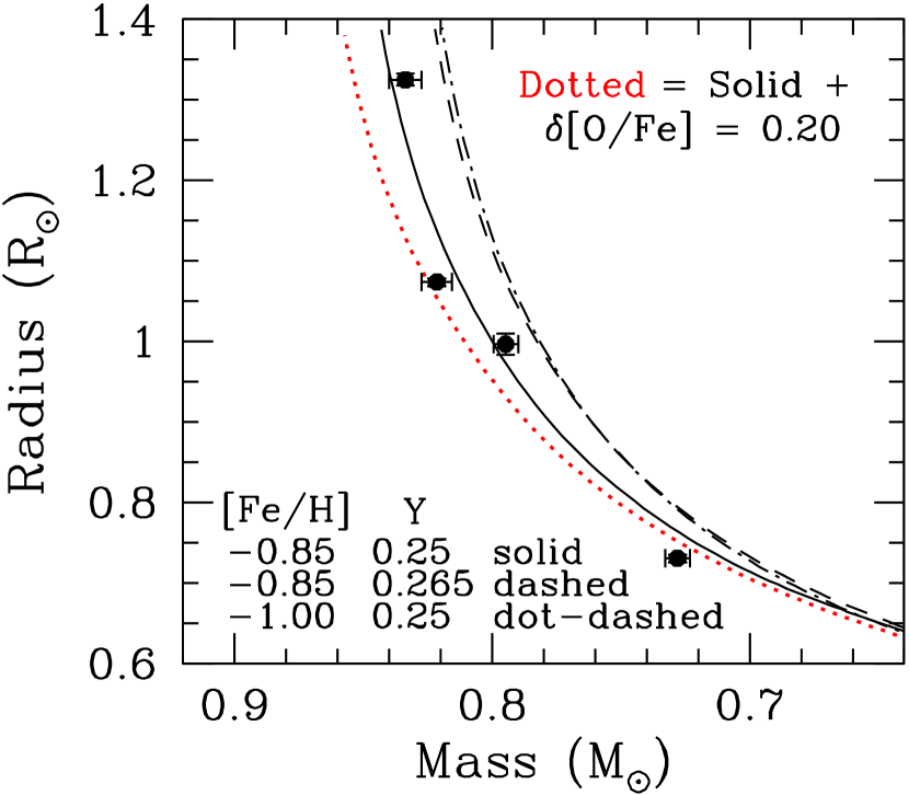
Figure 21.— Similar to the previous figure, except that isochrones for the indicated chemical abundances are compared with the observed masses and radii of V40 and V41.

Based on the results presented in Figs. 20 and 21, the binaries in NGC 6362 suggest that the cluster has [Fe/H] $=-0.90\pm 0.10$ and an oxygen abundance that is somewhere in the range $+0.4\leq$ [O/Fe] $\leq+0.6$. The effect on the predicted age of adopting a lower metallicity by 0.05 dex and a higher value of [O/Fe] by 0.1, relative to the metal abundances that were assumed in Fig. 18, is a reduction by about 0.2 Gyr. That is, our best estimate of the age of NGC 6362 is 12.4 Gyr. As for M 55, the uncertainty of this determination is $\approx\pm 0.8$ Gyr, of which $\pm 0.5$ Gyr is due to a $\pm 0.05$ mag uncertainty in the distance modulus and the rest corresponds to the net effect of metal abundance uncertainties.

Our results for M 55, NGC 6362, and the GCs considered in Papers I and II clearly depend on the reliability of our stellar models, especially those for the HB phase since they provide the basis for our adopted distance moduli. Consequently, it is important to check how well the predicted $(m-M)_{V}$ values agree with determinations based on other considerations. This is the subject of the next section.

5. Distance Constraints from Standard Candles

There have been a number of recent developments concerning the use of RR Lyrae and solar neighborhood subdwarfs as standard candles, but their implications for GC distances have not been very encouraging. In particular, the trigonometic parallaxes that have been derived for field RR Lyrae from first-epoch Gaia observations (Clementini et al. 2017) seem to favor a much shorter distance scale than the latest fits of GC main sequences to nearby subdwarfs; see Chaboyer et al. (2017) and O’Malley et al. (2017a), who made use of both the parallaxes that they derived from data taken with the HST Fine Guidance Sensors and those obtained from the Gaia mission (Gaia Collaboration et al. 2016) for a small number of stars. Since our HB models satisfy the RR Lyrae constraint quite well, as reported in Paper I, the main focus of this section will be on the subdwarf-fitting method. However, we will first compare the mean absolute magnitudes that we have derived for the RRab stars in several GCs with various empirical $M_{V}$–[Fe/H] relationships.

5.1. The RR Lyrae Standard Candle

Figure 22 plots the mean absolute magnitudes that we have derived for 6 GCs in Papers I–III of the present series as a function of their adopted metallicities. In order for our simulated HBs to match the properties of the observed ones, including the periods of the cluster RR Lyrae, these $\langle M_{V}\rangle$ values cannot be in error by more than $\sim\pm 0.05$ mag (the adopted error bar) if our models for the core He-burning phase are trustworthy. Current [Fe/H] estimates for most clusters are probably accurate to within $\sim\pm 0.1$ dex ($1\,\sigma$), though uncertainties closer to $\sim\pm 0.15$ dex appear to be more reasonable at the lowest metallicities (recall the discussion in §1). Accordingly, the horizontal error bars are larger for M 15 and M 92 than for the other clusters that are identified in Fig. 22. Superimposed on these data are several lines representing empirical calibrations that will now be discussed in turn.

The solid curve, which is defined by the equation $\langle M_{V}\rangle=0.57+0.214($[Fe/H] $+1.5)$, is widely considered to be the best empirical calibration of the RR Lyrae standard candle at the present time. This equation follows from the observed dependence of $\langle V_{0}\rangle$ on [Fe/H] that was obtained by Clementini et al. (2003) from their observations of $\sim 100$ variables in the Large Magellanic Cloud (LMC), if the very accurate LMC distance determined by Pietrzyński et al. (2013) from eclipsing binary stars is adopted. (The dashed lines are simply linear extensions of the solid curve outside the range in [Fe/H] spanned by the majority of the RR Lyrae in the Clementini et al. sample.) Incidently, our ZAHB models for [Fe/H] $=-2.0$ and $-1.4$, assuming $Y=0.25$, predict nearly the same slope as the solid curve, specifically, $\Delta M_{V}/$[Fe/H] $=0.220$ (versus 0.214; as noted at the beginning of this paragraph).

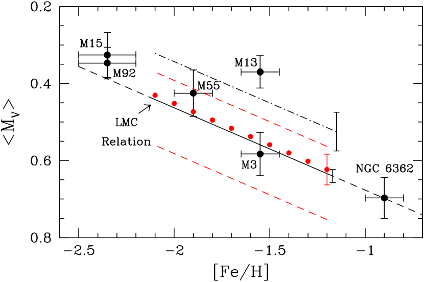
Figure 22.— RR Lyrae $M_{V}$ versus [Fe/H] relations from Clementini et al. (2003, solid line), Benedict et al. (2011, dot-dashed line), and Clementini et al. (2017, filled circles and dashed lines in red) together with our determinations of $\langle M_{V}\rangle$ for the variable stars in 6 GCs (filled circles with error bars). Black dashed lines provide linear extrapolations of the solid line to metallicities outside the range occupied by nearly all of LMC RR Lyrae that were observed by Clementini et al. (2003). These results assume that the true distance modulus of the LMC is $(m-M)_{0}=18.496$ (Pietrzyński et al. 2013). Note that the investigations by Benedict et al. (2011) and Clementini et al. (2017) both assumed $\Delta M_{V}/$[Fe/H] $=0.214$, as found by Clementini et al. (2003).

Using the Hubble Space Telescope Fine Guidance Sensors, Benedict et al. (2011) determined the trigonometric parallaxes of 5 RR Lyrae in the solar neighborhood, from which the dot-dashed relation and the attached error bar were derived. It assumes the same slope as the solid line, but a brighter zero-point by 0.12 mag. Perhaps the main concern with these results, aside from the small number of stars in the sample and the large uncertainties in the derived $M_{V}$ values (generally $\mathrel{\hbox{\raise 2.58334pt\hbox{$>$}\kern-7.3194pt\lower 2.15277pt\hbox{$\sim$}}}0.15$ mag, except in the case of RR Lyr itself) is the adoption of selection bias corrections (Lutz & Kelker 1973) ranging from $-0.02$ mag to $-0.11$ mag. Such corrections should not be applied to these stars according to Francis (2014).

The possibility that one (or two?) of the brightest stars are in a very different evolutionary state than the others would also have a significant effect on the derived $\langle M_{V}\rangle$–[Fe/H] relation when there are only a few variables in the sample, as in the Benedict et al. (2011) study. This concern is exemplified by our results for M 3 and M 13, which appear to have close to the same metallicity and age, but the mean absolute magnitudes of their RR Lyrae populations differ by more than 0.2 mag; see Fig. 22. This luminosity difference arises mainly because all of the RR Lyrae in M 13 are believed to be highly evolved stars from ZAHB locations well to the blue of the instability strip whereas a large fraction of the M 3 variables are located adjacent to the ZAHB. A difference in helium abundance (see Paper II) would also contribute to the luminosity offset.

Clementini et al. (2017) employed three different approaches in their analysis of preliminary Gaia observations for 200 field RR Lyrae (see their paper for details), finding zero-points that varied from 0.50 mag to 0.69 mag (at [Fe/H] $=-1.5$), if they assume the same slope of the $\langle M_{V}\rangle$ vs. [Fe/H] relation as in the aforementioned studies. Their application of a Bayesian fitting method yielded the relationship that has been plotted as the red filled circles in Fig. 22; the other two (represented by the red dashed lines) are offset by $-0.06$ mag and by $+0.13$ mag, respectively, at a given [Fe/H] value. The faintest of the three relations is considered by Clementini et al. to be the least trustworthy one because it involves the direct transformation of parallaxes into absolute magnitudes, which causes obviously asymmetric errors in the $M_{V}$ values when errors are large, besides being unable to take negative parallaxes into account. Although their preferred results agree quite well with those represented by the solid curve, more definitive findings will, as stated by the authors, have to await further studies of the systematic errors in the parallax determinations and improvements to the data that will accompany future releases of Gaia observations.

As reported in Paper I, and shown in Fig. 22, the mean absolute magnitude of M 3 RR Lyrae, assuming the distance modulus predicted by our ZAHB models and HB simulations, agrees with the value implied by the empirical $\langle M_{V}\rangle$–[Fe/H] relation from Clementini et al. (2003) to within $\sim 0.03$ mag. It is to be expected that the variables in M 55, and especially those in M 13, would lie above the same relation because they are predicted to be significantly more evolved stars and, in the case of M 13, to have somewhat higher $Y$, than those residing in M 3 (see Paper II). Since M 15 is especially rich in RR Lyrae, its location somewhat above the “LMC relation” (by only $1\,\sigma$, however) could also arise if it has a higher helium abundance in the mean than M 3 (see Paper I) or it may be a consequence of the assumed metallicity. If we had adopted [Fe/H] $=-2.5$ for M 15 (and M 92), as found in a number of recent studies (e.g., Sobeck et al. 2011, Roederer & Sneden 2011), we would have found that the RR Lyrae in both clusters lie on essentially the same $\langle M_{V}\rangle$ vs. [Fe/H] relation as those in M 3 (see Fig. 22). Indeed, we intend to examine in a forthcoming study whether it is possible to obtain a satisfactory explanation of the properties of the RR Lyrae in M 15 if they have a normal helium abundance but a very low metallicity. (Regardless of what the planned investigation reveals, we believe that a large spread in $Y$ is needed to explain the extended blue HB tails in such clusters as M 15 and M 13; see Paper II.)

Finally, the variables in NGC 6362 are predicted to lie just above the $\langle M_{V}\rangle$–[Fe/H] relationship that passes through the point representing M 3. This is consistent to well within the respective error bars with the prediction from our HB simulations that the RR Lyrae in NGC 6362 have a higher helium abundance than those in M 3 by $\Delta Y\sim 0.01$. In fact, it is unlikely that the variation of $\langle M_{V}\rangle$ with metallicity is strictly linear over the full range in [Fe/H] (see, e.g., the discussion by Catelan 2009); i.e., more metal-rich variables with the same $Y$ and evolutionary state are probably fainter than one would infer from a linear fit to the more metal-poor variables. Such a quadratic variation would tend to improve the consistency between theory and the observations of M 3 and NGC 6362. In any case, we can conclude from Fig. 22 that our models satisfy the RR Lyrae constraint very well. As a result, the distance moduli that we have derived for GCs in this series of papers, as well as those determined in the investigation by VandenBerg et al. (2013), should be accurate to within $\sim\pm 0.05$ mag ($1\,\sigma$).

5.2. The Local Subdwarf Standard Candle

VandenBerg et al. (2010) have already shown that the IRFM ${T_{\rm eff}}$ scale that was derived by CRMBA for solar neighborhood stars is nearly identical with that predicted by stellar models. Moreover, the same study (also see Brasseur et al. 2010) demonstrated that the colors of nearby dwarf stars are generally quite well reproduced when the models are transposed from the $(\log\,{T_{\rm eff}},\,M_{V})$-diagram to various CMDs using color transformations based on MARCS model atmospheres and synthetic spectra (specifically, the color–${T_{\rm eff}}$ relations presented in the subsequent study by Casagrande & VandenBerg 2014). This indicates that the predicted photometric properties of MARCS model atmospheres (Gustafsson et al. 2008) are able to match those of local dwarfs only if the temperatures of the latter are close to the values given by CRMBA (given the similarity of the stellar evolution and IRFM ${T_{\rm eff}}$ scales). The same can be said of dwarf stars in open and globular clusters since Victoria-Regina isochrones would not be able to reproduce the CMD morphologies of their MS populations so well (from their turnoffs at $M_{V}\sim 4$ to $M_{V}\mathrel{\hbox{\raise 2.58334pt\hbox{$>$}\kern-7.3194pt\lower 2.15277pt\hbox{$\sim$}}}8.5$; see VandenBerg et al. 2014a, their Figs. 9, 14, and 15) if they predicted much hotter or much cooler temperatures.

Figure 23.— Lower panel: superposition of the properties of nearby subdwarfs (filled circles) with [Fe/H] $\leq-1.3$ and $\sigma(M_{V})\leq 0.08$ mag onto 12.5 Gyr isochrones for $-2.6\leq$ [Fe/H] $\leq-1.2$, in $+0.2$ dex increments (from left to right). Aside from 3 stars with “BD” or “LTT” designations, the subdwarfs are identified by their HD numbers. Their absolute magnitudes are based on Gaia DR2 parallaxes, except in the case of HD 19445 (see the text) while their metallicities and effective temperatures have been taken from the study by CRMBA. The dashed curve represents the lower-MS portion of a solar abundance isochrone that provides an excellent fit to the morphology of the $[(V-K_{S})_{0},\,M_{V}]$ CMD of M 67 (VandenBerg et al. 2014a). The open circles and vertical error bars, which are comparable to the diameters of the open circles, indicate the locations of the subdwarfs that were studied by Chaboyer et al. (2017), assuming the properties derived by them. The filled square gives the location of HD 103095 if the temperature derived by Creevey et al. (2012) from CHARA interferometric observations is adopted. Middle panel: the difference, for each of the stars that has been plotted as a filled circle, between the [Fe/H] value adopted by CRMBA and that inferred from the interpolated (or extrapolated) isochrone that matches its location on the $(\log{T_{\rm eff}},\,M_{V})$-diagram (lower panel). The mean $\delta$ [Fe/H] value and the standard deviation are $-0.19$ dex and 0.25 dex, respectively (as indicated). Upper panel: similar to the middle panel, except that the difference between the CRMBA estimates of ${T_{\rm eff}}$ of each star and that predicted by the isochrone for its metallicity at the observed $M_{V}$ value.

It is worthwhile to revisit these findings in view of the very significant improvements that have been made to the absolute magnitudes of many of the most metal-deficient subdwarfs with the recent release of Gaia DR2 parallaxes. On the assumption of the effective temperatures given by CRMBA, the lower panel of Figure 23 compares the locations on the $(\log{T_{\rm eff}},\,M_{V})$-plane of 14 of the most metal-deficient subdwarfs (the filled circles) with Victoria-Regina isochrones (VandenBerg et al. 2014a) for $-2.6\leq$ [Fe/H] $\leq-1.2$. Although vertical error bars have been plotted, they are barely discernible, if at all, which indicates that the $M_{V}$ values are now sufficiently well determined that distance uncertainties are inconsequential; i.e., comparisons between theory and observations will be much more dependent on chemical compostion and ${T_{\rm eff}}$ uncertainties. Note that, because Gaia DR2 parallaxes are not available for HD 19445 at this time, we adopted the DR1 result (Gaia Collaboration et al. 2016) for this star. Encouragingly, all of the subdwarfs lie within, or just slightly outside, the band defined by the isochrones.

In fact, there is more than just qualitative consistency as the temperatures predicted by the evolutionary computations agree rather well with those derived by CRMBA. The top panel of Fig. 23 plots, for each subdwarf, the difference between the IRFM ${T_{\rm eff}}$ and the temperature predicted by an isochrone that has the same metallicity as the star (assuming the [Fe/H] value given by CRMBA), at its observed $M_{V}$ value. (The ${T_{\rm eff}}$ predicted by the models is readily obtained by interpolating within the grid of isochrones.) As indicated, the mean offset between the two is only 42 K, in the sense that the empirical temperatures tend to be cooler than those predicted by the models, with a standard deviation of 52 K. For 11 of the 14 subdwarfs, the observed minus isochrone (‘Obs–Iso’) ${T_{\rm eff}}$ differences are less than 50 K.

Alternatively, one can determine the difference between the subdwarf [Fe/H] value (from CRMBA) and that of the isochrone on which the subdwarf is located. As shown in the middle panel, the mean ‘Obs–Iso’ difference amounts to $-0.19$ dex, with a standard deviation of 0.25 dex, though the two estimates agree to within $\sim\pm 0.15$ dex for the majority of the stars in the sample. However, it should be appreciated that a small shift in the adopted temperature of any of the subdwarfs could imply a fairly large offset in its inferred [Fe/H] value from stellar models because the horizontal ($\log{T_{\rm eff}}$) separations between isochrones for metallicities that differ by 0.2 dex are small, especially at the lowest [Fe/H] values. At [Fe/H] $<-2$, a small change in ${T_{\rm eff}}$ implies a large difference in the inferred metallicity. Our point here is that the scale of the $\delta$ [Fe/H] variations may not be particularly meaningful. Obviously, the results presented in the top and middle panels are highly correlated.

In order to enlarge the sample of Population II stars in the solar neighborhood that can be used as standard candles, Chaboyer et al. (2017) determined very accurate and precise parallaxes for eight nearby subdwarfs with [Fe/H] $\mathrel{\hbox{\raise 2.58334pt\hbox{$<$}\kern-7.74998pt\lower 2.15277pt\hbox{$\sim$}}}-1.4$ using the HST Fine Guidance Sensors. The temperatures and metal abundances of these stars were determined by O’Malley et al. (2017a) via a differential chemical abundance analysis (relative to the Sun) of high-resolution, high signal-to-noise spectra. However, they found that the adoption of the color–${T_{\rm eff}}$ relations given by CRMBA resulted in steep slopes of the Fe I abundances with excitation potential, and that, to remove such trends, it was necessary to adopt cooler temperatures by as much as $\sim 400$ K than the photometric ${T_{\rm eff}}$ determinations. As shown in Fig. 23, where six of the subdwarfs are plotted as open circles, such low temperatures are highly problematic. In fact, the binaries in M 55 and NGC 6362 (recall Figs. 9 and 20) completely rule them out.

Compelling additional support for this conclusion is provided by the fact that the low ${T_{\rm eff}}$ values derived by O’Malley et al. (2017a) for 4 of the stars in their sample place them in close proximity to a 4.3 Gyr, solar abundance isochrone that matches the MS of M 67 on the $[(V-K)_{S},\,M_{V}]$-plane down to $M_{V}\sim 8.5$; see VandenBerg et al. (2014a, their Fig. 9). Indeed, the part of the isochrone that has been plotted is indistinguishable from one for 4.55 Gyr (the solar age) that passes through the location of the Sun on the same CMD or on the $(\log{T_{\rm eff}},\,M_{V})$-diagram. It is simply not possible that field subdwarfs with [Fe/H] $\mathrel{\hbox{\raise 2.58334pt\hbox{$<$}\kern-7.74998pt\lower 2.15277pt\hbox{$\sim$}}}-1.8$ have the same temperatures as MS stars in M 67 at the same absolute magnitudes. According to the constraints provided by the cluster binaries considered in this paper, the subdwarfs analyzed by O’Malley et al. cannot be much cooler than the predictions of stellar models for their metallicities (or IRFM-based temperatures), though they could be hotter than such estimates.

Apparently, the ${T_{\rm eff}}$ derived by Creevey et al. (2012) for HD 103095 ([Fe/H] $\sim-1.4$) from CHARA interferometric data suffers from the same problem (note the location of the filled square in Fig. 23). Indeed, concerns with the CHARA result have been expressed previously by Sitnova et al. (2015), who have found that such a low ${T_{\rm eff}}$ ($4818\pm 54$ K) is incompatible with all of the spectroscopic temperature indicators that they have checked (such as H_α line profiles). As noted by Heiter et al. (2015), the CHARA result is especially perplexing because most spectroscopic and photometric temperatures for HD 103095 have generally been in good agreement, favoring a value close to 5100 K.

The subgiant HD 140283 ([Fe/H] $\sim-2.5$) is another example of a Population II star in which the photometric ${T_{\rm eff}}$ value is considerably higher than the fundamental determination (see Heiter et al. 2015, VandenBerg et al. 2014b). Creevey et al. (2015) concluded that it is necessary to adopt a much smaller value of the mixing-length parameter than the solar value in order to explain the low ${T_{\rm eff}}$ that they derived from CHARA observations, but the CMDs of globular clusters with similar metallicities completely rule out this hypothesis (see § 3.2.2 in Paper I). More importantly, their temperature for HD 140283 would be in conflict with the unequivocal result from the eclipsing binary in M 55 in support of the IRFM and stellar model ${T_{\rm eff}}$ scales. Thus, there is substantial evidence (also see Casagrande et al. 2014) that some interferometric results suffer from systematic errors of one kind or another.

In any case, the adoption of what has turned out to be the wrong temperatures clearly calls into question the chemical abundances derived by O’Malley et al. (2017a), as well as the determination of GC distances and ages carried out by Chaboyer et al. (2017) on the basis of the subdwarfs in that sample. (Presumably, errors in the temperature structures of the model atmospheres used by O’Malley et al. are responsible for the dependence of Fe I abundance on excitation potential that led them to favor cool temperatures.) Although their abundance analysis should be repeated in order to derive improved metallicities, we note that several of the same subdwarfs were included in the spectroscopic survey carried out by Ishigaki et al. (2012), who adopted IRFM temperatures. Their [Fe/H] determinations are higher than those obtained by O’Malley et al. by up to $\sim 0.4$ dex, though there could well be other variations in the respective analysis methods that would serve to increase or decrease such differences.

Figure 24.— Similar to the previous figure, except that the subdwarfs are compared with isochrones that have been transposed to the $V-I_{C}$ color plane using the MARCS color–${T_{\rm eff}}$ relations (Casagrande & VandenBerg 2014). The colors and metallicities of the subdwarfs have been taken from the study by CRMBA, who claim that all of these stars are unreddened.

Since the MS-fitting method of determining GC distances involves comparisons of the apparent magnitudes of cluster stars with the $M_{V}$ values of local subdwarfs at the same intrinsic colors, rather than at common temperatures, it is instructive to compare the predicted and observed subdwarf properties on various CMDs. However, VandenBerg et al. (2010) have already shown that MARCS transformations to $B-V$ are considerably less successful than those for redder colors in satisfying observational constraints. Furthermore, redder colors have the advantage of being less sensitive to metal abundances than $B-V$, and since [Fe/H] determinations involve substantial uncertainties (recall Table 2 in § 1), we decided to focus on the $[(V-I_{C})_{0},\,M_{V}]$-diagram. It turns out that, as shown in Figure 24, Victoria-Regina isochrones (VandenBerg et al. 2014a) do a particularly fine job of reproducing the $V-I_{C}$ colors of the same 11 subdwarfs that were considered in the previous figure when they are transposed from the theoretical to the observed plane using MARCS color–${T_{\rm eff}}$ relations (from Casagrande & VandenBerg 2014); in both plots, they are represented by filled circles. The mean color offset turns out to be 0.01 mag and the standard deviation is 0.01 mag (see the upper panel). The differences between the [Fe/H] values given by CRMBA and those inferred from the isochrones are also small (see the middle panel).

Because the $\alpha$-element abundances affect both the predicted temperatures of stars (e.g., see VandenBerg et al. 2014a) and stellar color–${T_{\rm eff}}$ relations (Casagrande & VandenBerg 2014), the models that are compared with observations should assume the correct values of [$\alpha$/Fe] (though this is less of a concern at low metallicities and for $V-I_{C}$, rather than $B-V$, colors). As far as we have been able to determine, the subdwarfs used in this study have [$\alpha$/Fe] values quite close to $+0.4$, and we have therefore made use of isochrones for [$\alpha$/Fe] $=+0.4$ in Figs. 23 and 24. For instance, Casagrande et al. (2006) give [$\alpha$/Fe] values for HD 25329, HD 31128, HD 34328, HD 94028, and HD 145417 that vary from 0.33 to 0.49, with a mean value of 0.40, while the analysis of a high-resolution spectrum for HD 19445 by P. E. Nissen (see VandenBerg et al. 2014b) yielded [$\alpha$/Fe] $=0.39$.

The subdwarfs from the study by Chaboyer et al. (2017), which are plotted in Fig. 24 as open circles and identified by their Hipparcos catalog (HIP) numbers, do not line up in the way that they probably should. Even though the [Fe/H] values given by Chaboyer et al. (the numbers enclosed by parentheses) are almost certainly too low, it should still be the case that HIP 54639 and HIP 87788 are the most metal-deficient stars in their sample, and yet their locations on the $[(V-I_{C})_{0},\,M_{V}]$-diagram imply that they have significantly higher metallicities than HIP 46120 and HIP 108200. (Differences in the $\alpha$-element abundances could partially explain this, but Chaboyer et al. report that HIP 54639 has a lower value of [$\alpha$/Fe] than HIP 46120, which is in the wrong sense to explain the offset between these two stars.) Also, HIP 103269 and HIP 108200 should lie on the same isochrone if they have nearly the same [Fe/H] and [$\alpha$/Fe] values, as reported by Chaboyer et al. (something that needs to be checked by a follow-up spectroscopic study), but they do not do so. Even though Chaboyer have obtained very accurate distances for the subdwarfs in their sample, they are clearly of limited usefulness as standard candles at the present time because of problems with their effective temperatures and metallicities.

Interestingly, the most discrepant points in Fig. 23 (e.g., the one representing HD 25329) are much less problematic in Fig. 24. Their $(V-I)_{C}$ colors suggest, in fact, that the temperatures given by CRMBA for these stars may be too cool. Anyway, increasing their ${T_{\rm eff}}$ values by $\sim 100$ K, which is within the the $2\,\sigma$ uncertainties of the temperatures derived by CRMBA, would make their locations in the $[(\log{T_{\rm eff}},\,M_{V}]$-diagram much more consistent with the properties of the other subdwarfs in our sample.

5.2.1 The Subdwarf-Based Distance Modulus of M 55

Fortunately, Mandushev et al. (1996) have obtained deep $VI_{C}$ photometry for M 55, and we can therefore fit the MS fiducial that they derived to the local subdwarfs in order to determine the cluster distance modulus. We checked that their photometry is in good agreement with the observations that are publicly available for M 55 in P. Stetson’s “Photometric Standard Fields” archive (see footnote 3), and we found that the level of consistency between the two data sets is quite satisfactory. We then fitted a cubic to the fiducial points given by Mandushev et al. (from their Table 3), over the range in $V$ from 18.8 to 21.4, using a standard least-squares fitting code. When matching the cluster MS to the subdwarfs in the solar neighborhood, we will assume that the subdwarfs define a cubic with exactly the same linear, quadratic, and cubic coefficients as the one that has been fitted to the cluster photometry. The difference in the zero points (the constant terms) is $V-M_{V}$, which is the apparent distance modulus that we are seeking.

To produce a mono-metallicity subdwarf sequence for [Fe/H] $=-1.85$, which represents our best estimate of the metallicity of M 55 (see Fig. 12), the observed $V-I_{C}$ color for each of the 11 subdwarfs is adjusted by the difference in color, at its absolute $V$ magnitude, between an isochrone for [Fe/H] $=-1.85$ and one for the metallicity of the star. Thus, the colors of subdwarfs that are somewhat more metal-rich than M 55 will be shifted to slightly bluer $V-I_{C}$ colors, and vice versa. Note that the models are used in only a differential sense to determine these adjustments, which range from $-0.026$ mag in the case of HD 103095 and HD 145417 (the most metal-rich stars in our sample) to $+0.012$ mag in the case of BD$+$023375, which has the lowest metallicity. These corrections are quite minor because the horizontal separations between isochrones for different [Fe/H] values are small, which is the main (and important) advantage of performing this analysis on the $[(V-I_{C})_{0},\,M_{V}]$-diagram instead of the $[(B-V)_{0},\,M_{V}]$-plane.

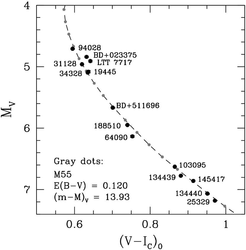
Figure 25.— Fit of the main-sequence fiducial of M 55 (gray dots connected by a dashed curve) to the 11 subdwarfs in our sample (filled circles with vertical error bars), once small corrections have been applied to their colors to compensate for the difference between their metallicities and that of the cluster (which is assumed to have [Fe/H] $=-1.85$). If $E(B-V)=0.120$, the MS fit yields $(m-M)_{V}=13.93$ (as indicated).

Once the mono-metallicity subdwarf sequence has been defined, one can use, e.g., the LFIT subroutine in Numerical Recipes (Press et al. 2007) to determine the zero-point of the cubic equation that provides the optimum fit to the subdwarfs, assuming that it has exactly the same shape as the one that has been fitted to the cluster MS. This particular computer program uses $\chi^{2}$ minimization to determine the value of the constant term, with each star given a weighting of $1/\sigma(M_{V})^{2}$. It turns out that $V-M_{V}=13.93$ if M 55 has [Fe/H] $=-1.85$ and $E(B-V)=0.12$; see Figure 25, which illustrates that the subdwarfs follow the morphology of the cluster MS fiducial rather well.

This determination depends much more on the reddening of M 55 than its metallicity. For instance, we would obtain $(m-M)_{V}=14.00$ if $E(B-V)=0.13$ and [Fe/H] $=-1.85$, as compared with 13.91 if $E(B-V)=0.12$ and [Fe/H] $=-2.00$. All of these results agree rather well with those found from fits of ZAHB models to the cluster HB stars (see Figs. 4 and 5), CMD simulations of the observed HB population (Fig. 6), and comparisons of the predicted and measured periods of the cluster RR Lyrae variables (see Table 4). Thus, nearly the same distance modulus is obtained for M 55 whether it is based on nearby subdwarfs, or the evolutionary and pulsational properties of the cluster HB stars. (As deep, high-quality $VI_{C}$ photometry has not yet been obtained for NGC 6362, as far as we are aware, we are not able to carry out a similar determination of its distance modulus as that just described for M 55.)

6. Summary

This investigation has presented a detailed analysis of the evolutionary and pulsational properties of the stars in M 55 and NGC 6362. These GCs were selected for the subject of this study because they contain detached, totally eclipsing binary stars with well determined masses and radii that can be used to constrain the chemical properties of the two clusters. Even more importantly, binaries are able to set tight limits on the ${T_{\rm eff}}$ scale of Population II stars, if their distances (and hence their luminosities) can be established to high accuracy and the uncertainties of their measured radii are small.

In this series of papers, we have used ZAHB models, simulated HBs, and comparisons of the predicted and observed periods of RR Lyrae variables to set the cluster distances. It is well known that the luminosities of HB stars depend on the envelope helium abundance, $Y_{\rm env}$, and the mass of the helium core, ${\cal M}_{c}^{\rm He}$. Metal-deficient GCs cannot have an initial He abundance, $Y_{0}$, that is less than the primordial value of $Y$ and, if diffusive processes are treated, the abundance of He in the convective envelopes of upper-RGB stars (i.e., after the first dredge-up) will be the lowest abundance that is predicted by stellar models ($Y_{\rm env}\mathrel{\hbox{\raise 2.58334pt\hbox{$<$}\kern-7.74998pt\lower 2.15277pt\hbox{$\sim$}}}Y_{0}$). Because RGBT models that neglect diffusion have values of $Y_{\rm env}$ that are larger than $Y_{0}$ by $\sim 0.01$–0.02 (see, e.g., Serenelli et al. 2017, their Table 2), the corresponding HB models will necessarily be brighter than those that treat this physics. (The fact that essentially the same distance modulus is obtained for M 3 from our HB models and from the best available calibration of the RR Lyrae standard candle provides a strong argument that diffusive processes cannot be ignored.) Moreover, any extra mixing processes that enhance $Y_{\rm env}$, or any non-canonical effects (e.g., rotation) that increase ${\cal M}_{c}^{\rm He}$, will also result in brighter HBs.

Based on these considerations, we would argue that the cluster distance moduli that we have derived from our HB computations cannot be much smaller than our determinations. (In fact, our estimates of $(m-M)_{V}$ appear to be quite accurate given that, in particular, a fit of the MS of M 55 to solar-neighborhood subdwarfs yields the same distance modulus for this GC to within $\sim 0.03$ mag.) On the assumption of the relatively short distance moduli obtained in this study, the temperatures that we have derived (from ${\cal L}=4\pi R^{2}\sigma{T_{\rm eff}}^{4})$ for the binaries in M 55 and NGC 6362 agree very well with those predicted by our isochrones — and with those inferred from the calibration of the IRFM by CRMBA. Any increase in the adopted values of $(m-M)_{V}$ would result in hotter temperatures.

This finding rules out the very cool temperatures that were found in the recent spectroscopic study of several field subdwarfs by O’Malley et al. (2017a), for instance, as well as those derived in some interferometric studies (e.g., Creevey et al. 2012, 2015). Such cool ${T_{\rm eff}}$ values as those reported in these investigations for stars with [Fe/H] $\mathrel{\hbox{\raise 2.58334pt\hbox{$<$}\kern-7.74998pt\lower 2.15277pt\hbox{$\sim$}}}-1.3$ present the additional difficulty that their location on the H-R diagram would place some of them on, or adjacent to, a solar-abundance, solar-age isochrone that satisfies the solar constraint. It is clear that determinations of the chemical abundances of Pop. II stars from their spectra must adopt relatively warm temperatures close to those favored by stellar models and the IRFM. Because detached, totally eclipsing binaries in GCs with well determined distances provide such powerful constraints on the ${T_{\rm eff}}$ scales, mass-radius relations, and mass-luminosity relations that apply to those clusters, efforts to discover and to observe such binaries should be given high priority and strong support. Once the temperatures are known, improvements to, among other things, metal abundance determinations, color–${T_{\rm eff}}$ relations, the temperature structures of model atmospheres, and (perhaps) to our understanding of convection theory, diffusion, and any other physics that can have a significant impact on the temperatures of stellar models will follow.

Our HB simulations indicate that both M 55 and NGC 6362 contain stars that span a small range in $Y$. We are able to reproduce the morphology and distribution of stars along the HB in M 55 if approximately half of them have $Y\approx 0.25$ and only $\sim 10$% have $Y\mathrel{\hbox{\raise 2.58334pt\hbox{$>$}\kern-7.3194pt\lower 2.15277pt\hbox{$\sim$}}}0.27$. The CMD for the HB stars in NGC 6362 is unusual insofar as the reddest non-variable stars are significantly fainter than the faintest RR Lyrae and non-variable stars just to the blue of the instability strip. These observations are readily explained if there are similar numbers of stars with $Y=0.25$, 0.265, and 0.28, and all of the RR Lyrae and bluer HB stars have enhanced helium abundances. Because the populations of HB stars with different $Y$ span such a wide color range, the luminosity offsets between them are easily seen, in contrast with the HBs of both more metal-rich and more metal-poor GCs, such as 47 Tuc (see Paper II) and M 55 (this paper). As a result, NGC 6362 provides one of the most striking examples of the existence of multiple stellar populations in globular clusters. Encouragingly, the reddest $ab$-type pulsators in NGC 6362 appear to follow the morphology (notably the blue loops) of post-ZAHB evolutionary tracks quite well.

Due to the spread in $Y$, the mass-radius and mass-luminosity diagrams for the binary components do not constrain the cluster metallicities particularly well because the effects of $\delta Y=0.02$ on predicted ${\cal M}$–${\cal R}$ and ${\cal M}$–$M_{V}$ relations is larger than the effects of a $+0.2$ dex change in [Fe/H]. As a result, the metallicity that is inferred from such plots depends on whether a particular binary belongs to the helium-normal or helium-enhanced population. Nevertheless, the binaries indicate that M 55 and NGC 6362 have [Fe/H] $\approx-1.85$ and $\approx-0.9$, respectively, with $1\sigma$ uncertainties amounting to $\sim 0.1$ dex. On the other hand, since we are using the HB to set the cluster distances, and the difference in the luminosity of the HB and the turnoff, $\Delta V_{TO}^{HB}$, to determine the cluster age, the uncertainty in the metallicity is not a serious concern; at higher [Fe/H] values, both the HB and the turnoff at a fixed age become fainter (though not by exactly the same amounts), and vice versa. Hence, as long as there is a significant population of stars with $Y=0.25$, to justify the use of HB models for this He abundance in determining the cluster distance, the effect of a 0.2 dex uncertainty in the metallicity on the derived age will be relatively minor.

If we adopt [O/Fe] $=0.5\pm 0.1$ and [$m$/H] $=0.4$ for the other $\alpha$-elements, we obtain $(m-M)_{V}=13.95\pm 0.05$ and an age of $12.9\pm 0.8$ Gyr for M 55, as compared with $(m-M)_{V}=14.56\pm 0.05$ and $12.4\pm 0.8$ Gyr for NGC 6362. The distance modulus uncertainty, which contributes $\approx\pm 0.5$ Gyr to the age uncertainty, corresponds to the range of possible values for which our models are able to reproduce the mean periods of the $ab$- and $c$-type RR Lyrae to within $\sim\pm 0.03$ days. The effects of chemical abundance uncertainties account for the remainder of the age uncertainty. The ages derived here for M 55 and NGC 6362 should be particularly robust because they are based on well-tested, up-to-date stellar models and they satisfy the constraints provided by member eclipsing binaries and RR Lyrae variables, as well as solar neighborhood subdwarfs (which were considered only in the case of M 55).

References

- Amarsi et al. (2016) Amarsi, A. M., Lind, K., Asplund, M., Barklem, P. S., & Collet, R. 2016, MNRAS, 463, 1518
- An et al. (2009) An, D., Pinsonneault, M. H., Masseron, T., et al. 2009, ApJ, 700, 523