Future Steps in Cosmology using Spectral Distortions of the Cosmic Microwave Background

Abstract

Since the measurements of COBE/FIRAS in the mid-90’s we know that the energy spectrum of the cosmic microwave background (CMB) is extremely close to that of a perfect blackbody at an average temperature $T_{0}\simeq 2.726\,{\rm K}$. However, a number of early-universe processes are expected to create CMB spectral distortions – departures of the average CMB energy spectrum from a blackbody – at a level that is within reach of present-day technology. This provides strong motivation to study the physics of CMB spectral distortions and ask what these small signals might be able to tell us about the Universe we live in. In this lecture, I will give a broad-brush overview of recent theoretical and experimental developments, explaining why future spectroscopic measurements of the CMB will open an unexplored new window to early-universe and particle physics. I will give an introduction about the different types of distortions, how they evolve and thermalize and highlight some of the physical processes that can cause them. I hope to be able to convince you that CMB spectral distortions could open an exciting new path forward in CMB cosmology, which is complementary to planned and ongoing searches for primordial B-mode polarization signals. Spectral distortions should thus be considered very seriously as part of the activities in the next decades.

1 Overview and motivation

Cosmology is now a precise scientific discipline, with detailed theoretical models that fit a wealth of very accurate measurements. Of the many cosmological data sets, the cosmic microwave background (CMB) temperature and polarization anisotropies provide the most stringent and robust constraints to theoretical models, allowing us to determine the key parameters of our Universe with unprecedented precision and address fundamental questions about inflation and early-universe physics. Clearly, by looking at the statistics of the CMB anisotropies with different experiments over the past decades we have learned a lot about the Universe we live in, entering the era of precision cosmology and establishing the $\Lambda$CDM concordance model [Smoot1992, WMAP_params, Planck2013params].

But the quest continues. Today we are in the position to ask exciting questions about extensions of the standard cosmological model [PRISM2013WPII, Abazajian2015Inf, Abazajian2015, Abazajian2016S4SB]. For instance, what do the CMB anisotropies tell us about Big Bang Nucleosynthesis (BBN) and in particular the primordial helium abundance, $Y_{\rm p}$? How many neutrino species are there in our Universe? This question is often addressed through the effective number of relativistic degree’s of freedom, $N_{\rm eff}$. What are the neutrino masses and their hierarchy? Are there some decaying or annihilating particles? What about dark radiation? And regarding the initial conditions of our Universe: what is the running of the power spectrum of curvature perturbations? How about the gravitational wave background, parametrized through the tensor-to-scalar ratio, $r$, which determines the energy scale of inflation, at least when assuming the standard inflation scenario. And to top it up, what about dark energy and the accelerated expansion of our Universe?

All these questions are extremely exciting and define todays cutting-edge research in cosmology, driving present-day theoretical and experimental efforts. The CMB anisotropies in combination with large-scale structure, weak lensing and supernova observations deliver ever more precise answers to these questions [Calabrese2013, Planck2015params]. But the CMB holds another, complementary and independent piece of invaluable information: its frequency spectrum. Departures of the CMB frequency spectrum from a pure blackbody – commonly referred to as spectral distortion – encode information about the thermal history of the early Universe (from when it was a few month old until today). Since the measurements with COBE/FIRAS in the early 90’s, the average CMB spectrum is known to be extremely close to a perfect blackbody at a temperature $T_{0}=(2.726\pm 0.001)\,{\rm K}$ [Fixsen1996, Fixsen2009] at redshift $z=0$, with possible distortions limited to one part in $10^{5}$. This impressive measurement was awarded the Nobel Prize in Physics 2006 and already rules out cosmologies with extended periods of significant energy release, disturbing the thermal equilibrium between matter and radiation in the Universe.

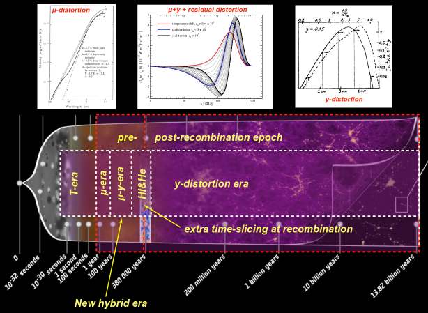
Figure 1: CMB spectral distortions probe the thermal history of the Universe at various stages during the pre- and post-recombination era. Energy release at $z\gtrsim\rm few\times 10^{6}$, when the Universe was only a few month old, merely causes a change of the CMB temperature. A $\mu$-type distortion arises from energy release at $3\times 10^{5}\lesssim z\lesssim\rm few\times 10^{6}$, while $y$-type distortions are created at $z\lesssim 10^{4}$. The signal caused during the $\mu/y$-transition era ($10^{4}\lesssim z\lesssim 3\times 10^{5}$) is described by a superposition of $\mu$- and $y$-distortion with some small residual distortion that allows probing the time-dependence of the energy-release mechanism. In the recombination era ($10^{3}\lesssim z\lesssim 10^{4}$), additional spectral features appear due to atomic transitions of hydrogen and helium. These could allow us to distinguish pre- from post-recombination $y$-distortions.

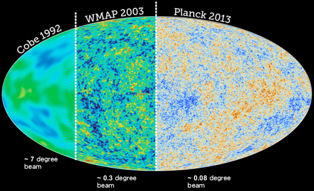
Figure 2: Over the past decades, CMB experiments have seen a dramatic improvement in sensitivity and angular resolution, illustrated here with a comparison of COBE, WMAP and PLANCK. In contrast, CMB spectral distortion measurements are still in the state of some 25 years ago, with COBE/FIRAS defining the unchallenged standard.

1.1 Why are spectral distortions so interesting today

So far no spectral distortion of the average CMB spectrum was found. Thus, why is it at all interesting to think about spectral distortions now? First of all, there is a long list of processes that could lead to spectral distortions. These include: reionization and structure formation; decaying or annihilating particles; dissipation of primordial density fluctuations; cosmic strings; primordial black holes; small-scale magnetic fields; adiabatic cooling of matter; cosmological recombination; and several new physics examples [Chluba2011therm, Sunyaev2013, Chluba2013fore, Tashiro2014, deZotti2015, Chluba2016]. This certainly makes theorists very happy, but most importantly, many of these processes (e.g., reionization and cosmological recombination) are part of our standard cosmological model and therefore should lead to guaranteed signals to search for. This shows that studies of spectral distortions offer both the possibility to constrain well-known physics but also to open up a discovery space for non-standard physics, potentially adding new time-dependent information to the picture (Fig. 1).

The second reason for spectral distortion being interesting is due to impressive technological advances since COBE. Although measurements of the CMB temperature and polarization anisotropies have improved significantly in terms of angular resolution and sensitivity since COBE/DMR, our knowledge of the CMB energy spectrum is still in a similar state as more than 25 years ago (Fig. 2). Already in 2002, improvements by a factor of $\simeq 100$ over COBE/FIRAS were deemed feasible [Fixsen2002], and today even more ambitious experimental concepts like PIXIE [Kogut2011PIXIE, Kogut2016SPIE] and PRISM [PRISM2013WPII], possibly reaching $\gtrsim 10^{3}$ in spectral sensitivity, are being seriously considered. These types of experiments provide a unique way to learn about processes that are otherwise hidden from us. At this stage, CMB spectral distortion measurements at high frequencies are furthermore only possible from space, so that, in contrast to $B$-mode polarization science, competition from the ground is largely excluded, making CMB spectral distortions a unique target for future CMB space missions [Chluba2014Science]. These efforts could be complemented from the ground at low frequencies ($\nu\lesssim 10\,{\rm GHz}$), targeting the cosmological recombination ripples, as suggested for APSERa [Mayuri2015], or $\mu$ and $y$-distortions using COSMO.

The immense potential of spectral distortions was realized in the NASA 30-year Roadmap study, where improved characterization of the CMB spectrum was declared as one of the future targets [Roadmap2014]. The strong synergy between spectral distortion and B-mode polarization measurements in terms of challenges related to foregrounds and systematic effects further motivate serious consideration of both science cases as part of the future experimental activities.

1.2 Overview and goal of the lecture

The main goal of the lectures is to convince you that CMB spectral distortion studies provide us with a new and immensely rich probe of early-universe physics, making it an exciting direction of cosmology for the future. These notes are based on extensive lectures on thermalization physics given as part of the CUSO lecture series in 2014, with extended lecture notes available at www.chluba.de/science. I will briefly review the physics of CMB spectral distortions, explaining the different types of distortions and how to compute them for different scenarios. I will then highlight different sources of distortions and what we might learn by measuring distortion signals in the future. Particular attention will be payed to the dissipation of small-scale perturbations and decaying particle scenarios, which illustrate the potential of distortion science. I will also briefly talk about the recombination era and the associated distortion signals and then mention a few of the challenges related to CMB foregrounds. This will also emphasize some of the synergies of distortion and B-mode searches.

2 The physics of CMB spectral distortions

In this section, I briefly review the main ingredients to describe CMB spectral distortions. The pioneering works on this topic are mainly due to Yakov Zeldovich and Rashid Sunyaev in the 60’s and 70’s [Zeldovich1969, Sunyaev1970mu, Illarionov1974, Illarionov1975]. These early works were later extended by [Danese1977, Danese1982], to include the effect of double Compton emission, and [Burigana1991, Hu1993], with refined numerical and analytical treatments. Latest considerations of spectral distortion and their science can be found in [Chluba2011therm, Sunyaev2013, Chluba2013fore, Tashiro2014, deZotti2015, Chluba2016] and [Jose2006, Sunyaev2009, Chluba2016Rec] for the recombination radiation.

2.1 Simple Blackbody relations

Before talking about CMB spectral distortions, let us briefly remind ourselves of a few important blackbody relations. We shall denote the blackbody intensity or Planckian as, $B_{\nu}(T)$, where $\nu$ is the frequency and $T$ the blackbody temperature. The Planck law reads:

$$B_{\nu}(T)=\frac{2h}{c^{2}}\frac{\nu^{3}}{{{\rm e}^{h\nu/kT}}-1}=\frac{2h\,\nu^{3}}{c^{2}}\,n^{\rm bb}_{\nu}(T)=I_{0}\,\frac{x^{3}}{{{\rm e}^{x}}-1},$$ (1)

having units $[B_{\nu}(T)]={\rm ergs}\sec^{-1}{\rm cm}^{-2}{\rm Hz}^{-1}{\rm sr}^{-1}=10^{17}\,{\rm MJy\,sr^{-1}}$. The spectrum of the Sun is approximately represented by this expression (let’s be a theorists and forget about all the Fraunhofer lines and existence of the atmosphere with all its absorption bands) with a temperature $T_{\rm ph}\simeq 6000\,{\rm K}$ (photosphere). Also, we already heard about the CMB blackbody spectrum, which is unbelievably close to a blackbody at a temperature $T_{0}=2.726\,{\rm K}$ [Fixsen1996, Fixsen2009].

In Eq. (1), we also indicate the connection of $B_{\nu}$ to the blackbody occupation number, $n^{\rm bb}_{\nu}(T)=1/({{\rm e}^{h\nu/kT}}-1)=1/({{\rm e}^{x}}-1)$, and transformed to the dimensionless frequency, $x=h\nu/kT$ (redshift-independent), introducing $I_{0}(T)=(2h/c^{2})(kT/h)^{3}\approx 270\,{\rm MJy\,sr^{-1}}(T/2.726{\rm K})^{3}$. It is useful to remember that $x=1$ corresponds to $\nu\approx 56.8\,{\rm GHz}$ for the CMB. Also, the maximum of the blackbody spectrum (Wien’s displacement law) is located at $\nu_{\rm max}\approx 160\,{\rm GHz}\left[\frac{T}{2.726\,{\rm K}}\right]$ or $x_{\rm max}\approx 2.821$. We furthermore have the important limiting cases

$$B_{\nu}(T)\approx\begin{cases}\frac{2\nu^{2}}{c^{2}}kT&\text{for}\;h\nu\ll kT\qquad\text{(Rayleigh-Jeans limit)},\\[5.69054pt] \frac{2h\nu^{3}}{c^{2}}{{\rm e}^{-h\nu/kT}}&\text{for}\;h\nu\gg kT\qquad\text{(Wien law)},\end{cases}$$ (2)

for the blackbody spectrum. In the Wien part of the spectrum, very few photons are found but their energy is large. The opposite is true in the Rayleigh-Jeans part.

2.2 Photon energy and number density

For our discussions, the total photon number and energy densities, $\rho_{\gamma}$ and $N_{\gamma}$, will be important. These are defined by the integrals, $\rho_{\gamma}=\int\frac{I_{\nu}}{c}{\,\rm d}\nu{\,\rm d}\Omega$ and $N_{\gamma}=\int\frac{I_{\nu}}{c\,h\nu}{\,\rm d}\nu{\,\rm d}\Omega$, over all photon energies and directions. Here, $I_{\nu}$ is the photon intensity. For blackbody radiation, this simply gives

$$\rho^{\rm Pl}_{\gamma} =\frac{2h}{c^{3}}\int\frac{\nu^{3}}{{{\rm e}^{x}}-1}{\,\rm d}\nu{\,\rm d}\Omega=\frac{8\pi h}{c^{3}}\left(\frac{kT}{h}\right)^{4}\int\frac{x^{3}{\,\rm d}x}{{{\rm e}^{x}}-1}=\frac{8\pi^{5}(kT)^{4}}{15\,c^{3}h^{3}}$$

$$=a_{R}T^{4}\approx 5.10\times 10^{-7}\,m_{\rm e}c^{2}{\rm cm}^{-3}\left(\frac{T}{2.726{\rm K}}\right)^{4}\approx 0.26\,{\rm eV}\,{\rm cm}^{-3}\left(\frac{T}{2.726{\rm K}}\right)^{4}$$ (3a)

$$N^{\rm Pl}_{\gamma} =\frac{2}{c^{3}}\int\frac{\nu^{2}}{{{\rm e}^{x}}-1}{\,\rm d}\nu{\,\rm d}\Omega=\frac{8\pi}{c^{3}}\left(\frac{kT}{h}\right)^{3}\int\frac{x^{2}{\,\rm d}x}{{{\rm e}^{x}}-1}=\frac{16\pi\zeta_{3}(kT)^{3}}{c^{3}h^{3}}$$

$$=b_{R}T^{3}\approx 410\,{\rm cm}^{-3}\left(\frac{T}{2.726{\rm K}}\right)^{3},$$ (3b)

where $\zeta_{i}$ denotes the Riemann $\zeta$-function. Here, $a_{R}=4\sigma/c\approx 7.566\times 10^{-15}\,{\rm ergs}\,{\rm cm}^{-3}\,{\rm K}^{-4}$ is the radiation constant, where $\sigma$ is the Stefan-Boltzmann constant. We also have the useful relation $\rho^{\rm Pl}_{\gamma}\approx 2.701kTN^{\rm Pl}_{\gamma}$. In particular, we have $\rho^{\rm Pl}_{\gamma}\propto T^{4}$ and $N^{\rm Pl}_{\gamma}\propto T^{3}$, the crucial blackbody relations.

2.3 What do we need to do to change the blackbody temperature

The blackbody spectrum is fully characterized by one number, its temperature $T$. Thus, one simple question is, what do we have to do to shift the temperature to $T^{\prime}\neq T$? Let’s suppose we increase the temperature by adding some energy to the photon field (let’s say we just move all photons upwards in frequency in some way; no change of the volume or photon number), $\epsilon=\Delta\rho_{\gamma}/\rho_{\gamma}^{\rm Pl}(T)\equiv(T^{\prime}/T)^{4}-1$, then the expected change in the photon temperature is

$$\frac{\Delta T}{T}=\left(1+\epsilon\right)^{1/4}-1\approx\frac{1}{4}\frac{\Delta\rho_{\gamma}}{\rho_{\gamma}^{\rm Pl}},$$ (4)

for small $\Delta\rho_{\gamma}/\rho_{\gamma}^{\rm Pl}$. Clearly, if we stopped here, the new spectrum cannot be a blackbody anymore, since we did not change the photon number density. Thus, pure energy release/extraction inevitably leads to a spectral distortion, no matter how the photons are distributed in energy.

To keep the blackbody relation, $N^{\rm Pl}_{\gamma}\propto T^{3}$, unchanged we simultaneously need to add

$$\frac{\Delta N_{\gamma}}{N_{\gamma}^{\rm Pl}}=(T^{\prime}/T)^{3}-1=(1+\epsilon)^{3/4}-1\approx 3\frac{\Delta T}{T}\quad\Longrightarrow\quad\frac{\Delta N_{\gamma}}{N_{\gamma}^{\rm Pl}}\approx\frac{3}{4}\frac{\Delta\rho_{\gamma}}{\rho_{\gamma}^{\rm Pl}}$$ (5)

of photons to avoid creating a non-blackbody spectrum. This condition is necessary but not sufficient, since it does not specify how the missing photons are distributed in energy! For example, let us assume we add photons to the blackbody spectrum at one frequency only. Then $\Delta\rho_{\gamma}=h\nu\Delta N_{\gamma}$ and $\epsilon\approx(h\nu/2.701kT)\,\Delta N_{\gamma}/N_{\gamma}^{\rm Pl}$. To satisfy the condition Eq. (5), we just need to tune the frequency to $h\nu/kT\approx(4/3)\,2.70\approx 3.60$. Clearly, a blackbody spectrum with a single narrow line at $h\nu\simeq 3.6\,kT$ is no longer a blackbody even if Eq. (5) is satisfied. We thus also need to add photons to the CMB spectrum in just the right way and the question is how?

To go from one blackbody with temperature $T$ to another at temperature $T^{\prime}$, we need to have a change of the photon occupation number by

$$\Delta n_{\nu}=n_{\rm bb}(T^{\prime})-n_{\rm bb}(T)=\frac{1}{{{\rm e}^{x^{\prime}}}-1}-\frac{1}{{{\rm e}^{x}}-1}=-x\partial_{x}n_{\rm bb}\,\frac{\Delta T}{T}+\mathcal{O}\left(\frac{\Delta T}{T}\right)^{2}=\frac{x{{\rm e}^{x}}}{({{\rm e}^{x}}-1)^{2}}\,\frac{\Delta T}{T}+\mathcal{O}\left(\frac{\Delta T}{T}\right)^{2}$$

with $x^{\prime}=x\,T/T^{\prime}$. In what follows, we will frequently use the definition

$$G(x)=-x\partial_{x}n_{\rm bb}=\frac{x\,{{\rm e}^{x}}}{({{\rm e}^{x}}-1)^{2}}\approx\begin{cases}\frac{1}{x}&\text{for}\qquad x\ll 1\\ x\,{{\rm e}^{-x}}&\text{for}\qquad x\gg 1,\end{cases}$$ (6)

which determines the spectrum of a temperature shift: $T\partial_{T}B_{\nu}\propto x^{3}G(x)$, for small $\Delta T/T$. Its spectral shape is shown in Fig. LABEL:fig:Y_SZ_and_mu_distortion. It is easy to prove that a change with this spectral distribution does not lead to any distortion as long as $\Delta T/T$ is sufficiently small. We will thus refer to $G(x)$ as the spectrum of a temperature shift. In the thermalization problem, it is created through the combined action of Compton scattering and photon creation processes (i.e., double Compton and Bremsstrahlung emission).

2.4 What is the thermalization problem all about

When considering the cosmological thermalization problem we are asking: how was the present CMB spectrum really created? Assuming that everything starts off with a pure blackbody spectrum, the uniform adiabatic expansion of the Universe alone (absolutely no collisions and spatial perturbations here!) leaves this spectrum unchanged – a blackbody thus remains a blackbody at all times. However, as the simple discussion in the proceeding section already showed, processes leading to photon production/destruction or energy release/extraction should inevitably introduce momentary distortions to the CMB spectrum. Then the big question is: was there enough time from the creation of the distortion until today to fully restore the blackbody shape, pushing distortions below any observable level? For this, we need to redistribute photons in energy through Compton scattering by free electrons. However, this is not enough to restore the blackbody spectrum. We also need to adjust the number of photons through double Compton and Bremsstrahlung. By understanding the thermalization problem and studying the CMB spectrum in fine detail we can thus learn about different early-universe processes and the thermal history of our Universe. This can open a new window to the early Universe, allowing us to peek behind the last scattering surface which is so important for the formation of the CMB temperature and polarization anisotropies.

2.5 General conditions relevant to the thermalization problem

In the early Universe, photons undergo many interactions with the other particles. We shall mainly concern ourselves with the average CMB spectrum and neglect distortion anisotropies when describing their evolution. Distortion anisotropies can be created through anisotropic energy release processes; however, these are usually very small, such that we only briefly touch on them below. We also assume that the distortions are always minor in amplitude, so that the problem can be linearized. This allows us to resort to a Green’s function approach when solving the thermalization problem [Chluba2013Green, Chluba2015GreenII], which greatly simplifies explicit thermalization calculations for different energy release scenarios as can be carried out using the full thermalization code CosmoTherm [Chluba2011therm].

We furthermore assume the standard $\Lambda$CDM background cosmology [Planck2015params] with standard ionization history computed using CosmoRec [Chluba2010b]. Also, the electron and baryon distribution functions are given by Maxwellians at a common temperature, $T_{\rm e}$, down to very low redshifts ($z\lesssim 10$), when thermalization process is already extremely inefficient. We furthermore need not worry about the evolution of distortions before the electron-positron annihilation era ($z\gtrsim 10^{7}-10^{8}$), since in this regime rapid thermalization processes always ensure that the CMB spectrum is very close to that of a blackbody. We are thus just dealing with non-relativistic electrons, protons and helium nuclei immersed in a bath of CMB photons. We can also neglect the traces of other light elements for the thermalization problem and usually assume that neutrinos and dark matter are only important for determining the expansion rate of the Universe.

2.6 Photon Boltzmann equation for average spectrum

The study of the formation and evolution of CMB fluctuations in both real and frequency space begins with the radiative transport, or Boltzmann equation for the photon phase space distribution, $n(x^{\mu},p^{\mu})$. Here, we are only interested in the evolution of the average spectrum. In this case, perturbations can be neglected, such that $n(x^{\mu},p^{\mu})\rightarrow n(t,p)$ and we may express the photon Boltzmann equation as

$$\frac{\partial n}{\partial t}-H\,p\frac{\partial n}{\partial p}={\rm C}[n],$$ (7)

omitting the any spatial dependence. Here, $H(t)$ is the standard Hubble expansion rate and ${\rm C}[n]$ denotes the collision term, which accounts for interactions of photons with the other species in the Universe. The collision term incorporates several important effects. Most importantly, Compton scattering couples photons and electrons, keeping the two in close thermal contact until low redshifts, $z\lesssim 100-200$. Bremsstrahlung and double Compton emission allow adjusting the photon number and are especially fast at low frequencies, as we explain below.

Neglecting collisions (${\rm C}[n]=0$), we directly recover $n(t,p)=n[t_{0},p\,a(t)/a(t_{0})]$, which means that the shape of the photon distribution is conserved by the universal expansion and only the photon momenta are redshifted. Introducing the variable $x=p/kT_{\gamma}(t)=h\nu/kT_{\gamma}(t)$, with $T_{\gamma}(t)=T_{\gamma}(t_{0})\,a(t_{0})/a(t)\propto(1+z)$, the photon Boltzmann equation takes the more compact form $\partial n(t,x)/\partial t={\rm C}[n(t,x)]$ (see [Chluba2011therm] for more details), which highlights the conservation law.

2.7 Collision term for Compton scattering

We already mentioned that Compton scattering is responsible for redistributing photons in energy. This problem has been studied a lot in connection with X-rays from compact objects