A Systematic Expansion of Running Couplings and Masses
F.A. Chishtie
Department of Physics and Astronomy, The
University of Western Ontario, London, ON N6A 5B7, Canada
Corresponding author
D.G.C. McKeon
Department of Physics and Astronomy, The
University of Western Ontario, London, ON N6A 5B7, Canada
Department of Mathematics and
Computer Science, Algoma University,
T.N. Sherry
School of Mathematics, Statistics and Applied Mathematics, National University of Ireland Galway, University Road, Galway H91 TK33 Ireland
Abstract
As an alternative to directly integrating their defining equations to find the running coupling a ( μ ) 𝑎 𝜇 a(\mu) m ( μ ) 𝑚 𝜇 m(\mu) ln ( μ μ ′ ) 𝜇 superscript 𝜇 ′ \ln\left(\frac{\mu}{\mu^{\prime}}\right) a ( μ ′ ) 𝑎 superscript 𝜇 ′ a(\mu^{\prime}) m ( μ ′ ) 𝑚 superscript 𝜇 ′ m(\mu^{\prime}) M S ¯ ¯ 𝑀 𝑆 \overline{MS}
PACS No.: 11.10Hi
Two essential ingredients of quantum chromodynamics are the running coupling a ( μ ) 𝑎 𝜇 a(\mu) m ( μ ) 𝑚 𝜇 m(\mu)
μ d a ( μ ) d μ 𝜇 𝑑 𝑎 𝜇 𝑑 𝜇 \displaystyle\mu\frac{da(\mu)}{d\mu} = β ( a ) = − b a 2 ( 1 + c a + c 2 a 2 + c 3 a 3 + … ) absent 𝛽 𝑎 𝑏 superscript 𝑎 2 1 𝑐 𝑎 subscript 𝑐 2 superscript 𝑎 2 subscript 𝑐 3 superscript 𝑎 3 … \displaystyle=\beta(a)=-ba^{2}\left(1+ca+c_{2}a^{2}+c_{3}a^{3}+\ldots\right) (1a)
μ d m ( μ ) d μ 𝜇 𝑑 𝑚 𝜇 𝑑 𝜇 \displaystyle\mu\frac{dm(\mu)}{d\mu} = m γ ( a ) = m f a ( 1 + g 1 a + g 2 a 2 + … ) , absent 𝑚 𝛾 𝑎 𝑚 𝑓 𝑎 1 subscript 𝑔 1 𝑎 subscript 𝑔 2 superscript 𝑎 2 … \displaystyle=m\gamma(a)=mfa\left(1+g_{1}a+g_{2}a^{2}+\ldots\right), (1b)
where c i subscript 𝑐 𝑖 c_{i} g i subscript 𝑔 𝑖 g_{i} ( i + 1 ) 𝑖 1 (i+1)
a ¯ ¯ 𝑎 \displaystyle\overline{a} = a + x 2 a 2 + x 3 a 3 + … absent 𝑎 subscript 𝑥 2 superscript 𝑎 2 subscript 𝑥 3 superscript 𝑎 3 … \displaystyle=a+x_{2}a^{2}+x_{3}a^{3}+\ldots (2a)
m ¯ ¯ 𝑚 \displaystyle\overline{m} = ( 1 + y 1 a + y 2 a 2 + … ) absent 1 subscript 𝑦 1 𝑎 subscript 𝑦 2 superscript 𝑎 2 … \displaystyle=\left(1+y_{1}a+y_{2}a^{2}+\ldots\right) (2b)
only the coefficients b 𝑏 b c 𝑐 c f 𝑓 f M S ¯ ¯ 𝑀 𝑆 \overline{MS} g i ( i = 1 , 2 , 3 , 4 ) subscript 𝑔 𝑖 𝑖 1 2 3 4
g_{i}\left(i=1,2,3,4\right) c i ( i = 2 , 3 , 4 ) subscript 𝑐 𝑖 𝑖 2 3 4
c_{i}(i=2,3,4) a ( μ ) 𝑎 𝜇 a(\mu) m ( μ ) 𝑚 𝜇 m(\mu)
ln ( μ Λ ) 𝜇 Λ \displaystyle\ln\left(\frac{\mu}{\Lambda}\right) = ∫ 0 a ( μ ) d x β ( x ) + ∫ 0 ∞ d x b x 2 ( 1 + c x ) absent superscript subscript 0 𝑎 𝜇 𝑑 𝑥 𝛽 𝑥 superscript subscript 0 𝑑 𝑥 𝑏 superscript 𝑥 2 1 𝑐 𝑥 \displaystyle=\int_{0}^{a(\mu)}\frac{dx}{\beta(x)}+\int_{0}^{\infty}\frac{dx}{bx^{2}(1+cx)} (3a)
m ( μ ) 𝑚 𝜇 \displaystyle m(\mu) = I M exp ( ∫ 0 a ( μ ) d x γ ( x ) β ( x ) + ∫ 0 ∞ d x f x b x 2 ( 1 + c x ) ) absent 𝐼 𝑀 superscript subscript 0 𝑎 𝜇 𝑑 𝑥 𝛾 𝑥 𝛽 𝑥 superscript subscript 0 𝑑 𝑥 𝑓 𝑥 𝑏 superscript 𝑥 2 1 𝑐 𝑥 \displaystyle=I\!\!M\exp\left(\int_{0}^{a(\mu)}\frac{dx\gamma(x)}{\beta(x)}+\int_{0}^{\infty}\frac{dxfx}{bx^{2}(1+cx)}\right) (3b)
where Λ Λ \Lambda I M 𝐼 𝑀 I\!\!M a 𝑎 a m 𝑚 m
In our approach, we utilize the expansions
a ′ superscript 𝑎 ′ \displaystyle a^{\prime} = a [ 1 + ( α 11 ℓ ) a + ( α 21 ℓ + α 22 ℓ 2 ) a 2 + … ] absent 𝑎 delimited-[] 1 subscript 𝛼 11 ℓ 𝑎 subscript 𝛼 21 ℓ subscript 𝛼 22 superscript ℓ 2 superscript 𝑎 2 … \displaystyle=a\left[1+\left(\alpha_{11}\ell\right)a+\left(\alpha_{21}\ell+\alpha_{22}\ell^{2}\right)a^{2}+\ldots\right] (4a)
m ′ superscript 𝑚 ′ \displaystyle m^{\prime} = m [ 1 + ( β 11 ℓ ) a + ( β 21 ℓ + β 22 ℓ 2 ) a 2 + … ] absent 𝑚 delimited-[] 1 subscript 𝛽 11 ℓ 𝑎 subscript 𝛽 21 ℓ subscript 𝛽 22 superscript ℓ 2 superscript 𝑎 2 … \displaystyle=m\left[1+\left(\beta_{11}\ell\right)a+\left(\beta_{21}\ell+\beta_{22}\ell^{2}\right)a^{2}+\ldots\right] (4b)
where a ′ = a ( μ ′ ) superscript 𝑎 ′ 𝑎 superscript 𝜇 ′ a^{\prime}=a(\mu^{\prime}) m ′ = m ( μ ′ ) superscript 𝑚 ′ 𝑚 superscript 𝜇 ′ m^{\prime}=m(\mu^{\prime}) a = a ( μ ) 𝑎 𝑎 𝜇 a=a(\mu) m = m ( μ ) 𝑚 𝑚 𝜇 m=m(\mu) ℓ = ln ( μ μ ′ ) ℓ 𝜇 superscript 𝜇 ′ \ell=\ln\left(\frac{\mu}{\mu^{\prime}}\right) a ′ superscript 𝑎 ′ a^{\prime} m ′ superscript 𝑚 ′ m^{\prime} a 𝑎 a m 𝑚 m a ′ superscript 𝑎 ′ a^{\prime} m ′ superscript 𝑚 ′ m^{\prime} μ 𝜇 \mu
μ d a ′ d μ 𝜇 𝑑 superscript 𝑎 ′ 𝑑 𝜇 \displaystyle\mu\frac{da^{\prime}}{d\mu} = 0 = ( μ ∂ ∂ μ + β ( a ) ∂ ∂ a ) a ′ absent 0 𝜇 𝜇 𝛽 𝑎 𝑎 superscript 𝑎 ′ \displaystyle=0=\left(\mu\frac{\partial}{\partial\mu}+\beta(a)\frac{\partial}{\partial a}\right)a^{\prime} (5a)
μ d m ′ d μ 𝜇 𝑑 superscript 𝑚 ′ 𝑑 𝜇 \displaystyle\mu\frac{dm^{\prime}}{d\mu} = 0 = ( μ ∂ ∂ μ + β ( a ) ∂ ∂ a + m γ ( a ) ∂ ∂ m ) m ′ . absent 0 𝜇 𝜇 𝛽 𝑎 𝑎 𝑚 𝛾 𝑎 𝑚 superscript 𝑚 ′ \displaystyle=0=\left(\mu\frac{\partial}{\partial\mu}+\beta(a)\frac{\partial}{\partial a}+m\gamma(a)\frac{\partial}{\partial m}\right)m^{\prime}. (5b)
If, in eq. (4), we define
a ′ superscript 𝑎 ′ \displaystyle a^{\prime} = ∑ n = 0 ∞ S n ( a l ) a n + 1 absent superscript subscript 𝑛 0 subscript 𝑆 𝑛 𝑎 𝑙 superscript 𝑎 𝑛 1 \displaystyle=\sum_{n=0}^{\infty}S_{n}(al)a^{n+1} (6a)
m ′ superscript 𝑚 ′ \displaystyle m^{\prime} = m ∑ n = 0 ∞ T n ( a l ) a n absent 𝑚 superscript subscript 𝑛 0 subscript 𝑇 𝑛 𝑎 𝑙 superscript 𝑎 𝑛 \displaystyle=m\sum_{n=0}^{\infty}T_{n}(al)a^{n} (6b)
where S n ( ξ ) = ∑ k = 0 ∞ α n + k , k ξ k subscript 𝑆 𝑛 𝜉 superscript subscript 𝑘 0 subscript 𝛼 𝑛 𝑘 𝑘
superscript 𝜉 𝑘 S_{n}(\xi)=\sum_{k=0}^{\infty}\alpha_{n+k,k}\xi^{k} T n ( ξ ) = ∑ k = 0 ∞ β n + k , k ξ k subscript 𝑇 𝑛 𝜉 superscript subscript 𝑘 0 subscript 𝛽 𝑛 𝑘 𝑘
superscript 𝜉 𝑘 T_{n}(\xi)=\sum_{k=0}^{\infty}\beta_{n+k,k}\xi^{k} α n , 0 = β n , 0 = δ n , 0 subscript 𝛼 𝑛 0
subscript 𝛽 𝑛 0
subscript 𝛿 𝑛 0
\alpha_{n,0}=\beta_{n,0}=\delta_{n,0}
( μ ∂ ∂ μ + β ( a ) ∂ ∂ a ) ∑ n = 0 ∞ S n ( a ℓ ) a n + 1 𝜇 𝜇 𝛽 𝑎 𝑎 superscript subscript 𝑛 0 subscript 𝑆 𝑛 𝑎 ℓ superscript 𝑎 𝑛 1 \displaystyle\left(\mu\frac{\partial}{\partial\mu}+\beta(a)\frac{\partial}{\partial a}\right)\sum_{n=0}^{\infty}S_{n}(a\ell)a^{n+1} = 0 absent 0 \displaystyle=0 (7a)
( μ ∂ ∂ μ + β ( a ) ∂ ∂ a + m γ ( a ) ∂ ∂ m ) ∑ n = 0 ∞ m T n ( a ℓ ) a n 𝜇 𝜇 𝛽 𝑎 𝑎 𝑚 𝛾 𝑎 𝑚 superscript subscript 𝑛 0 𝑚 subscript 𝑇 𝑛 𝑎 ℓ superscript 𝑎 𝑛 \displaystyle\left(\mu\frac{\partial}{\partial\mu}+\beta(a)\frac{\partial}{\partial a}+m\gamma(a)\frac{\partial}{\partial m}\right)\sum_{n=0}^{\infty}mT_{n}(a\ell)a^{n} = 0 . absent 0 \displaystyle=0. (7b)
Together, eqs. (1,7) result in a pair of sets of nested equations - one set for S n subscript 𝑆 𝑛 S_{n}
( 1 − b ξ ) S 0 ′ 1 𝑏 𝜉 superscript subscript 𝑆 0 ′ \displaystyle(1-b\xi)S_{0}^{\prime} − b S 0 = 0 𝑏 subscript 𝑆 0 0 \displaystyle-bS_{0}=0 (8a)
( 1 − b ξ ) S 1 ′ 1 𝑏 𝜉 superscript subscript 𝑆 1 ′ \displaystyle(1-b\xi)S_{1}^{\prime} − 2 b S 1 − b c ( S 0 ′ ξ + S 0 ) = 0 ; 2 𝑏 subscript 𝑆 1 𝑏 𝑐 superscript subscript 𝑆 0 ′ 𝜉 subscript 𝑆 0 0 \displaystyle-2bS_{1}-bc\left(S_{0}^{\prime}\xi+S_{0}\right)=0; (8b)
and the second set for T n subscript 𝑇 𝑛 T_{n}
( 1 − b ξ ) T 0 ′ + f T 0 1 𝑏 𝜉 superscript subscript 𝑇 0 ′ 𝑓 subscript 𝑇 0 \displaystyle(1-b\xi)T_{0}^{\prime}+fT_{0} = 0 absent 0 \displaystyle=0 (9a)
( 1 − b ξ ) T 1 ′ + ( f − b ) T 1 1 𝑏 𝜉 superscript subscript 𝑇 1 ′ 𝑓 𝑏 subscript 𝑇 1 \displaystyle(1-b\xi)T_{1}^{\prime}+(f-b)T_{1} − b c T 0 ′ ξ + f g 1 T 0 = 0 . 𝑏 𝑐 superscript subscript 𝑇 0 ′ 𝜉 𝑓 subscript 𝑔 1 subscript 𝑇 0 0 \displaystyle-bcT_{0}^{\prime}\xi+fg_{1}T_{0}=0. (9b)
In general the equation for S n subscript 𝑆 𝑛 S_{n} ( S 0 … S n − 1 ) subscript 𝑆 0 … subscript 𝑆 𝑛 1 (S_{0}\ldots S_{n-1}) ( b , c , c 2 … c n ) 𝑏 𝑐 subscript 𝑐 2 … subscript 𝑐 𝑛 (b,c,c_{2}\ldots c_{n}) T n subscript 𝑇 𝑛 T_{n} ( T 0 … T n − 1 ) subscript 𝑇 0 … subscript 𝑇 𝑛 1 (T_{0}\ldots T_{n-1}) ( b , c , c 2 … c n , f , g 0 … g n ) 𝑏 𝑐 subscript 𝑐 2 … subscript 𝑐 𝑛 𝑓 subscript 𝑔 0 … subscript 𝑔 𝑛 (b,c,c_{2}\ldots c_{n},f,g_{0}\ldots g_{n}) S n ( 0 ) = T n ( 0 ) = δ n , 0 subscript 𝑆 𝑛 0 subscript 𝑇 𝑛 0 subscript 𝛿 𝑛 0
S_{n}(0)=T_{n}(0)=\delta_{n,0}
S 0 subscript 𝑆 0 \displaystyle S_{0} = 1 w ( w = 1 − b ξ ) absent 1 𝑤 𝑤 1 𝑏 𝜉
\displaystyle=\frac{1}{w}\qquad(w=1-b\xi) (10a)
S 1 subscript 𝑆 1 \displaystyle S_{1} = − c ln w w 2 absent 𝑐 𝑤 superscript 𝑤 2 \displaystyle=\frac{-c\ln w}{w^{2}} (10b)
S 2 subscript 𝑆 2 \displaystyle S_{2} = c 2 ( ln 2 w − ln w + w − 1 ) − c 2 ( w − 1 ) w 3 absent superscript 𝑐 2 superscript 2 𝑤 𝑤 𝑤 1 subscript 𝑐 2 𝑤 1 superscript 𝑤 3 \displaystyle=\frac{c^{2}\left(\ln^{2}w-\ln w+w-1\right)-c_{2}(w-1)}{w^{3}} (10c)
S 3 subscript 𝑆 3 \displaystyle S_{3} = 1 2 w 4 [ − 2 c 3 ln 3 w + 5 c 3 ln 2 w − 4 { ( − 1 + w ) c 2 − c 2 ( w − 3 2 ) } c ln w \displaystyle=\frac{1}{2w^{4}}\Big{[}-2c^{3}\ln^{3}w+5c^{3}\ln^{2}w-4\left\{(-1+w)c^{2}-c_{2}\left(w-\frac{3}{2}\right)\right\}c\ln w
− ( − 1 + w ) { ( − 1 + w ) c 3 − 2 c c 2 w + c 3 ( w + 1 ) } ] \displaystyle\hskip 56.9055pt-(-1+w)\left\{(-1+w)c^{3}-2cc_{2}w+c_{3}(w+1)\right\}\Big{]} (10d)
S 4 = 1 6 w 5 [ 6 c 4 ln 4 w − 26 c 4 ln 3 w + { 18 c 2 ( c 2 − c 2 ) w − 9 c 2 ( c 2 − 4 c 2 ) } ln 2 w \displaystyle S_{{4}}=\frac{1}{6{w}^{5}}\Big{[}6\,{c}^{4}\ln^{4}w-26\,{c}^{4}\ln^{3}w+\left\{18\,{c}^{2}\left({c}^{2}-c_{{2}}\right)w-9\,{c}^{2}\left({c}^{2}-4\,c_{{2}}\right)\right\}\ln^{2}w
+ { 6 c ( c 3 − 2 c c 2 + c 3 ) w 2 − 30 c 2 ( c 2 − c 2 ) w + 6 c ( 4 c 3 − 3 c c 2 − 2 c 3 ) } ln w 6 𝑐 superscript 𝑐 3 2 𝑐 subscript 𝑐 2 subscript 𝑐 3 superscript 𝑤 2 30 superscript 𝑐 2 superscript 𝑐 2 subscript 𝑐 2 𝑤 6 𝑐 4 superscript 𝑐 3 3 𝑐 subscript 𝑐 2 2 subscript 𝑐 3 𝑤 \displaystyle+\left\{6\,c\left({c}^{3}-2\,cc_{{2}}+c_{{3}}\right){w}^{2}-30\,{c}^{2}\left({c}^{2}-c_{{2}}\right)w+6\,c\left(4\,{c}^{3}-3\,cc_{{2}}-2\,c_{{3}}\right)\right\}\ln w
+ ( 2 c 4 − 6 c 2 c 2 + 4 c 3 c + 2 c 2 2 − 2 c 4 ) w 3 + ( 3 c 4 − 6 c 2 c 2 − 3 c 3 c + 6 c 2 2 ) w 2 2 superscript 𝑐 4 6 subscript 𝑐 2 superscript 𝑐 2 4 subscript 𝑐 3 𝑐 2 superscript subscript 𝑐 2 2 2 subscript 𝑐 4 superscript 𝑤 3 3 superscript 𝑐 4 6 subscript 𝑐 2 superscript 𝑐 2 3 subscript 𝑐 3 𝑐 6 superscript subscript 𝑐 2 2 superscript 𝑤 2 \displaystyle+\left(2\,{c}^{4}-6\,c_{{2}}{c}^{2}+4\,c_{{3}}c+2\,{c_{{2}}}^{2}-2\,c_{{4}}\right){w}^{3}+\left(3\,{c}^{4}-6\,c_{{2}}{c}^{2}-3\,c_{{3}}c+6\,{c_{{2}}}^{2}\right){w}^{2}
− ( 12 c 2 − 18 c 2 ) ( c 2 − c 2 ) w + 7 c 4 − 18 c 2 c 2 − c 3 c + 10 c 2 2 + 2 c 4 ] \displaystyle-\left(12\,{c}^{2}-18\,c_{{2}}\right)\left({c}^{2}-c_{{2}}\right)w+7\,{c}^{4}-18\,c_{{2}}{c}^{2}-c_{{3}}c+10\,{c_{{2}}}^{2}+2\,c_{{4}}\Big{]} (10e)
T 0 subscript 𝑇 0 \displaystyle T_{0} = w ρ ( ρ = f / b ) absent superscript 𝑤 𝜌 𝜌 𝑓 𝑏
\displaystyle=w^{\rho}\qquad(\rho=f/b) (10f)
T 1 subscript 𝑇 1 \displaystyle T_{1} = − ρ w − 1 + ρ [ − c ln w + ( c − g 1 ) ( w − 1 ) ] absent 𝜌 superscript 𝑤 1 𝜌 delimited-[] 𝑐 𝑤 𝑐 subscript 𝑔 1 𝑤 1 \displaystyle=-\rho w^{-1+\rho}\left[-c\ln w+(c-g_{1})(w-1)\right] (10g)
T 2 subscript 𝑇 2 \displaystyle T_{2} = ρ 2 w − 2 + ρ [ − c 2 ( 1 − ρ ) ln 2 w + { − 2 ρ ( c − g 1 ) ( w − 1 ) + 2 g 1 } c ln w \displaystyle=\frac{\rho}{2}w^{-2+\rho}\bigg{[}-c^{2}(1-\rho)\ln^{2}w+\left\{-2\rho(c-g_{1})(w-1)+2g_{1}\right\}c\ln w (10h)
+ ( w − 1 ) { ( c 2 − c 2 + ρ ( c − g 1 ) 2 ) ( w − 1 ) + ( g 2 − c g 1 ) ( w + 1 ) } ] . \displaystyle+(w-1)\left\{\left(c^{2}-c_{2}+\rho(c-g_{1})^{2}\right)(w-1)+\left(g_{2}-cg_{1}\right)(w+1)\right\}\bigg{]}.
For T 3 subscript 𝑇 3 T_{3} T 4 subscript 𝑇 4 T_{4}
It is possible to verify that if eq. (10) is used to express a ( μ ′′ ) 𝑎 superscript 𝜇 ′′ a(\mu^{\prime\prime}) a ( μ ′ ) 𝑎 superscript 𝜇 ′ a(\mu^{\prime}) a ( μ ′ ) 𝑎 superscript 𝜇 ′ a(\mu^{\prime}) a ( μ ) 𝑎 𝜇 a(\mu) a ( μ ′′ ) 𝑎 superscript 𝜇 ′′ a(\mu^{\prime\prime}) a ( μ ) 𝑎 𝜇 a(\mu)
μ ′ d d μ ′ a ( μ ′ ) superscript 𝜇 ′ 𝑑 𝑑 superscript 𝜇 ′ 𝑎 superscript 𝜇 ′ \displaystyle\mu^{\prime}\frac{d}{d\mu^{\prime}}a(\mu^{\prime}) = β ( a ( μ ′ ) ) absent 𝛽 𝑎 superscript 𝜇 ′ \displaystyle=\beta(a(\mu^{\prime})) (11a)
μ ′ d m ( μ ′ ) d μ ′ superscript 𝜇 ′ 𝑑 𝑚 superscript 𝜇 ′ 𝑑 superscript 𝜇 ′ \displaystyle\mu^{\prime}\frac{dm(\mu^{\prime})}{d\mu^{\prime}} = m ( μ ′ ) γ ( a ( μ ′ ) ) . absent 𝑚 superscript 𝜇 ′ 𝛾 𝑎 superscript 𝜇 ′ \displaystyle=m(\mu^{\prime})\gamma(a(\mu^{\prime})). (11b)
These two consistency checks are most easily verified if the expansion coefficients α m n subscript 𝛼 𝑚 𝑛 \alpha_{mn} β m n subscript 𝛽 𝑚 𝑛 \beta_{mn}
When using the ’t Hooft renormalization scheme [17] we set c i = 0 ( i ≥ 2 ) subscript 𝑐 𝑖 0 𝑖 2 c_{i}=0(i\geq 2) g i = 0 ( i ≥ 1 ) subscript 𝑔 𝑖 0 𝑖 1 g_{i}=0(i\geq 1) S n subscript 𝑆 𝑛 S_{n} T n subscript 𝑇 𝑛 T_{n} f ˙ ≡ d d w f ( w ) ˙ 𝑓 𝑑 𝑑 𝑤 𝑓 𝑤 \dot{f}\equiv\frac{d}{dw}f(w)
S ˙ n + ( n + 1 ) w S n + c [ ( 1 − 1 w ) S ˙ n − 1 + n w S n − 1 ] subscript ˙ 𝑆 𝑛 𝑛 1 𝑤 subscript 𝑆 𝑛 𝑐 delimited-[] 1 1 𝑤 subscript ˙ 𝑆 𝑛 1 𝑛 𝑤 subscript 𝑆 𝑛 1 \displaystyle\dot{S}_{n}+\frac{(n+1)}{w}S_{n}+c\left[\left(1-\frac{1}{w}\right)\dot{S}_{n-1}+\frac{n}{w}S_{n-1}\right] = 0 absent 0 \displaystyle=0 (12a)
T ˙ n + ( n − ρ ) w T n + c [ ( 1 − 1 w ) T ˙ n − 1 + n − 1 w T n − 1 ] subscript ˙ 𝑇 𝑛 𝑛 𝜌 𝑤 subscript 𝑇 𝑛 𝑐 delimited-[] 1 1 𝑤 subscript ˙ 𝑇 𝑛 1 𝑛 1 𝑤 subscript 𝑇 𝑛 1 \displaystyle\dot{T}_{n}+\frac{(n-\rho)}{w}T_{n}+c\left[\left(1-\frac{1}{w}\right)\dot{T}_{n-1}+\frac{n-1}{w}T_{n-1}\right] = 0 . absent 0 \displaystyle=0. (12b)
Upon setting w n + 1 S n = c n σ n superscript 𝑤 𝑛 1 subscript 𝑆 𝑛 superscript 𝑐 𝑛 subscript 𝜎 𝑛 w^{n+1}S_{n}=c^{n}\sigma_{n}
σ n ( w ) subscript 𝜎 𝑛 𝑤 \displaystyle\sigma_{n}(w) = f n − 1 ( w ) − ( − 1 ) n + 1 − n ∫ 1 w d x x f n − 1 ( x ) ( n = 1 , 2 … ) absent subscript 𝑓 𝑛 1 𝑤 superscript 1 𝑛 1 𝑛 superscript subscript 1 𝑤 𝑑 𝑥 𝑥 subscript 𝑓 𝑛 1 𝑥 𝑛 1 2 …
\displaystyle=f_{n-1}(w)-(-1)^{n+1}-n\int_{1}^{w}\frac{dx}{x}f_{n-1}(x)\quad(n=1,2\ldots) (13a)
where σ 0 = 1 subscript 𝜎 0 1 \sigma_{0}=1
f n − 1 ( x ) subscript 𝑓 𝑛 1 𝑥 \displaystyle f_{n-1}(x) = σ n − 1 ( x ) − x σ n − 2 ( x ) + x 2 σ n − 3 ( x ) + … + ( − 1 ) n + 1 x n − 1 σ 0 ( x ) absent subscript 𝜎 𝑛 1 𝑥 𝑥 subscript 𝜎 𝑛 2 𝑥 superscript 𝑥 2 subscript 𝜎 𝑛 3 𝑥 … superscript 1 𝑛 1 superscript 𝑥 𝑛 1 subscript 𝜎 0 𝑥 \displaystyle=\sigma_{n-1}(x)-x\sigma_{n-2}(x)+x^{2}\sigma_{n-3}(x)+\ldots+(-1)^{n+1}x^{n-1}\sigma_{0}(x) (13b)
while from eq. (11b), if w n − ρ T n = c n τ n superscript 𝑤 𝑛 𝜌 subscript 𝑇 𝑛 superscript 𝑐 𝑛 subscript 𝜏 𝑛 w^{n-\rho}T_{n}=c^{n}\tau_{n} ( n = 0 , 1 , … ) 𝑛 0 1 …
(n=0,1,\ldots)
d d w τ n + ( w − 1 ) d d w τ n − 1 + ρ ( 1 − 1 w ) τ n − 1 + n − 1 w τ n − 1 = 0 . 𝑑 𝑑 𝑤 subscript 𝜏 𝑛 𝑤 1 𝑑 𝑑 𝑤 subscript 𝜏 𝑛 1 𝜌 1 1 𝑤 subscript 𝜏 𝑛 1 𝑛 1 𝑤 subscript 𝜏 𝑛 1 0 \frac{d}{dw}\tau_{n}+(w-1)\frac{d}{dw}\tau_{n-1}+\rho\left(1-\frac{1}{w}\right)\tau_{n-1}+\frac{n-1}{w}\tau_{n-1}=0. (14)
It thus proves relatively easy to obtain S n subscript 𝑆 𝑛 S_{n} T n subscript 𝑇 𝑛 T_{n} T 3 subscript 𝑇 3 T_{3} T 4 subscript 𝑇 4 T_{4}
T 3 = 1 6 w ρ − 3 ρ c 3 ( ln w − w + 1 ) [ ( ρ − 1 ) ( ρ − 2 ) ln 2 w + ( − ( 2 ρ − 2 ) ( ρ + 1 ) w + 2 ρ 2 − 5 ) ln w \displaystyle T_{{3}}=\frac{1}{6}{w}^{\rho-3}\rho\,{c}^{3}(\ln w-w+1)\Big{[}(\rho-1)(\rho-2)\ln^{2}w+(-(2\,\rho-2)(\rho+1)w+2\,{\rho}^{2}-5)\ln w
+ ( ρ + 2 ) ( ρ + 1 ) w 2 + ( − 2 ρ 2 − 6 ρ − 1 ) w + ρ 2 + 3 ρ − 1 ] \displaystyle+(\rho+2)(\rho+1){w}^{2}+(-2\,{\rho}^{2}-6\,\rho-1)w+{\rho}^{2}+3\,\rho-1\Big{]} (15a)
T 4 = 1 24 w ρ − 4 ρ c 4 ( ln w − w + 1 ) [ ( ρ − 1 ) ( ρ − 2 ) ( ρ − 3 ) ( ln 3 w + ( − ( 3 ρ − 3 ) ( ρ − 2 ) ( ρ + 1 ) w \displaystyle T_{{4}}=\frac{1}{24}\,{w}^{\rho-4}\rho\,{c}^{4}(\ln w-w+1)\Big{[}(\rho-1)(\rho-2)(\rho-3)(\ln^{3}w+(-(3\,\rho-3)(\rho-2)(\rho+1)w
+ 3 ρ 3 − 6 ρ 2 − 15 ρ + 26 ) ( ln 2 w + { ( 3 ρ − 3 ) ( ρ + 2 ) ( ρ + 1 ) w 2 + ( − 6 ρ 3 − 12 ρ 2 + 30 ρ + 8 ) w + 3 ρ 3 \displaystyle+3\,{\rho}^{3}-6\,{\rho}^{2}-15\,\rho+26)(\ln^{2}w+\{(3\,\rho-3)(\rho+2)(\rho+1){w}^{2}+(-6\,{\rho}^{3}-12\,{\rho}^{2}+30\,\rho+8)w+3\,{\rho}^{3}
+ 6 ρ 2 − 27 ρ − 2 } ln w − ( ρ + 3 ) ( ρ + 2 ) ( ρ + 1 ) w 3 + ( 3 ρ 3 + 18 ρ 2 + 21 ρ + 2 ) w 2 \displaystyle+6\,{\rho}^{2}-27\,\rho-2\}\ln w-(\rho+3)(\rho+2)\left(\rho+1\right){w}^{3}+\left(3\,{\rho}^{3}+18\,{\rho}^{2}+21\,\rho+2\right){w}^{2}
+ ( − 3 ρ 3 − 18 ρ 2 − 9 ρ + 14 ) w + ρ 3 + 6 ρ 2 − ρ − 10 ) ] \displaystyle+\left(-3\,{\rho}^{3}-18\,{\rho}^{2}-9\,\rho+14\right)w+{\rho}^{3}+6\,{\rho}^{2}-\rho-10)\Big{]} (15b)
In the ’t Hooft RS, eqs. (3a,b) can be integrated to obtain
m 𝑚 \displaystyle m = I M f b ln ( 1 + c a c a ) absent 𝐼 𝑀 𝑓 𝑏 1 𝑐 𝑎 𝑐 𝑎 \displaystyle=\frac{I\!\!Mf}{b}\ln\left(\frac{1+ca}{ca}\right) (16a)
and
ζ 𝜁 \displaystyle\zeta + ln ζ = 1 + b c ln ( μ Λ ) 𝜁 1 𝑏 𝑐 𝜇 Λ \displaystyle+\ln\zeta=1+\frac{b}{c}\ln\left(\frac{\mu}{\Lambda}\right) (16b)
where ζ ≡ 1 + 1 c a 𝜁 1 1 𝑐 𝑎 \zeta\equiv 1+\frac{1}{ca} a ( ln μ Λ ) 𝑎 𝜇 Λ a\left(\ln\frac{\mu}{\Lambda}\right) w ( x ) ( w e w = x ) 𝑤 𝑥 𝑤 superscript 𝑒 𝑤 𝑥 w(x)(we^{w}=x)
It is possible to express a ¯ ¯ 𝑎 \overline{a} m ¯ ¯ 𝑚 \overline{m} c ¯ i subscript ¯ 𝑐 𝑖 \overline{c}_{i} g ¯ i subscript ¯ 𝑔 𝑖 \overline{g}_{i} a 𝑎 a m 𝑚 m c i subscript 𝑐 𝑖 c_{i} g i subscript 𝑔 𝑖 g_{i}
∂ a ∂ c i = B i ( a ) 𝑎 subscript 𝑐 𝑖 subscript 𝐵 𝑖 𝑎 \displaystyle\frac{\partial a}{\partial c_{i}}=B_{i}(a) = − b β ( a ) ∫ 0 a 𝑑 x x i + 2 β 2 ( x ) absent 𝑏 𝛽 𝑎 superscript subscript 0 𝑎 differential-d 𝑥 superscript 𝑥 𝑖 2 superscript 𝛽 2 𝑥 \displaystyle=-b\beta(a)\int_{0}^{a}dx\frac{x^{i+2}}{\beta^{2}(x)} (17a)
≈ a i + 1 [ 1 i − 1 − c ( i − 2 i ( i − 1 ) ) a + 1 i + 1 ( c 2 i − 2 i − c 2 i − 3 i − 1 ) a 2 + … ] absent superscript 𝑎 𝑖 1 delimited-[] 1 𝑖 1 𝑐 𝑖 2 𝑖 𝑖 1 𝑎 1 𝑖 1 superscript 𝑐 2 𝑖 2 𝑖 subscript 𝑐 2 𝑖 3 𝑖 1 superscript 𝑎 2 … \displaystyle\approx a^{i+1}\left[\frac{1}{i-1}-c\left(\frac{i-2}{i(i-1)}\right)a+\frac{1}{i+1}\left(c^{2}\frac{i-2}{i}-c_{2}\frac{i-3}{i-1}\right)a^{2}+\ldots\right]
∂ a ∂ g i 𝑎 subscript 𝑔 𝑖 \displaystyle\frac{\partial a}{\partial g_{i}} = 0 absent 0 \displaystyle=0 (17b)
1 m ∂ m ∂ c i = Γ i c ( a ) 1 𝑚 𝑚 subscript 𝑐 𝑖 superscript subscript Γ 𝑖 𝑐 𝑎 \displaystyle\frac{1}{m}\frac{\partial m}{\partial c_{i}}=\Gamma_{i}^{c}(a) = γ ( a ) β ( a ) β ( a ) + b ∫ 0 a 𝑑 x x i + 2 γ ( x ) β 2 ( x ) absent 𝛾 𝑎 𝛽 𝑎 𝛽 𝑎 𝑏 superscript subscript 0 𝑎 differential-d 𝑥 superscript 𝑥 𝑖 2 𝛾 𝑥 superscript 𝛽 2 𝑥 \displaystyle=\frac{\gamma(a)}{\beta(a)}\beta(a)+b\int_{0}^{a}dx\frac{x^{i+2}\gamma(x)}{\beta^{2}(x)} (17c)
≈ ρ a i [ − 1 i ( i − 1 ) + 2 ( c i ( i + 1 ) − g 1 ( i + 1 ) ( i − 1 ) ) a \displaystyle\approx\rho a^{i}\bigg{[}\frac{-1}{i(i-1)}+2\left(\frac{c}{i(i+1)}-\frac{g_{1}}{(i+1)(i-1)}\right)a
+ 1 i + 2 ( 2 c 2 − 3 c 2 i + 1 + 4 g 1 c i − 3 g 2 i − 1 ) a 3 + … ] \displaystyle+\frac{1}{i+2}\left(\frac{2c_{2}-3c^{2}}{i+1}+\frac{4g_{1}c}{i}-\frac{3g_{2}}{i-1}\right)a^{3}+\ldots\bigg{]}
and
1 m ∂ m ∂ g i 1 𝑚 𝑚 subscript 𝑔 𝑖 \displaystyle\frac{1}{m}\frac{\partial m}{\partial g_{i}} = Γ i g ( a ) = f ∫ 0 a 𝑑 x x i + 1 β ( x ) absent superscript subscript Γ 𝑖 𝑔 𝑎 𝑓 superscript subscript 0 𝑎 differential-d 𝑥 superscript 𝑥 𝑖 1 𝛽 𝑥 \displaystyle=\Gamma_{i}^{g}(a)=f\int_{0}^{a}dx\frac{x^{i+1}}{\beta(x)} (17d)
= f b a i [ − 1 i + ( c i + 1 ) a + ( c 2 − c 2 i + 2 ) a 2 \displaystyle=\frac{f}{b}a^{i}\bigg{[}-\frac{1}{i}+\left(\frac{c}{i+1}\right)a+\left(\frac{c_{2}-c^{2}}{i+2}\right)a^{2}
+ ( c 3 + c 3 − 2 c c 2 i + 3 ) a 3 + ( c 4 − c 4 + 2 c 2 c 2 − 2 c c 3 − c 2 2 i + 4 ) a 4 + … ] . \displaystyle+\left(\frac{c_{3}+c^{3}-2cc_{2}}{i+3}\right)a^{3}+\left(\frac{c_{4}-c^{4}+2c^{2}c_{2}-2cc_{3}-c_{2}^{2}}{i+4}\right)a^{4}+\ldots\bigg{]}.
If we now expand
a ¯ ¯ 𝑎 \displaystyle\overline{a} = a [ 1 + ϕ 1 ( c j , c ¯ j ) a + ϕ 2 ( c j , c ¯ j ) a 2 + … ] absent 𝑎 delimited-[] 1 subscript italic-ϕ 1 subscript 𝑐 𝑗 subscript ¯ 𝑐 𝑗 𝑎 subscript italic-ϕ 2 subscript 𝑐 𝑗 subscript ¯ 𝑐 𝑗 superscript 𝑎 2 … \displaystyle=a\left[1+\phi_{1}\left(c_{j},\overline{c}_{j}\right)a+\phi_{2}\left(c_{j},\overline{c}_{j}\right)a^{2}+\ldots\right] (18a)
m ¯ ¯ 𝑚 \displaystyle\overline{m} = m [ 1 + ψ 1 ( c j , c ¯ j ; g j , g ¯ j ) a + ψ 2 ( c j , c ¯ j ; g j , g ˙ j ) a 2 + … ] absent 𝑚 delimited-[] 1 subscript 𝜓 1 subscript 𝑐 𝑗 subscript ¯ 𝑐 𝑗 subscript 𝑔 𝑗 subscript ¯ 𝑔 𝑗 𝑎 subscript 𝜓 2 subscript 𝑐 𝑗 subscript ¯ 𝑐 𝑗 subscript 𝑔 𝑗 subscript ˙ 𝑔 𝑗 superscript 𝑎 2 … \displaystyle=m\left[1+\psi_{1}\left(c_{j},\overline{c}_{j};g_{j},\overline{g}_{j}\right)a+\psi_{2}\left(c_{j},\overline{c}_{j};g_{j},\dot{g}_{j}\right)a^{2}+\ldots\right] (18b)
where ϕ i ( c j , c j ; g j , g j ) = 0 = ψ i ( c j , c j ; g j , g j ) subscript italic-ϕ 𝑖 subscript 𝑐 𝑗 subscript 𝑐 𝑗 subscript 𝑔 𝑗 subscript 𝑔 𝑗 0 subscript 𝜓 𝑖 subscript 𝑐 𝑗 subscript 𝑐 𝑗 subscript 𝑔 𝑗 subscript 𝑔 𝑗 \phi_{i}\left(c_{j},c_{j};g_{j},g_{j}\right)=0=\psi_{i}\left(c_{j},c_{j};g_{j},g_{j}\right)
d a ¯ d c i 𝑑 ¯ 𝑎 𝑑 subscript 𝑐 𝑖 \displaystyle\frac{d\overline{a}}{dc_{i}} = ( ∂ ∂ c i + B i ( a ) ∂ ∂ a ) a ¯ = 0 absent subscript 𝑐 𝑖 subscript 𝐵 𝑖 𝑎 𝑎 ¯ 𝑎 0 \displaystyle=\left(\frac{\partial}{\partial c_{i}}+B_{i}(a)\frac{\partial}{\partial a}\right)\overline{a}=0 (19a)
d a ¯ d g i 𝑑 ¯ 𝑎 𝑑 subscript 𝑔 𝑖 \displaystyle\frac{d\overline{a}}{dg_{i}} = 0 absent 0 \displaystyle=0 (19b)
d m ¯ d c i 𝑑 ¯ 𝑚 𝑑 subscript 𝑐 𝑖 \displaystyle\frac{d\overline{m}}{dc_{i}} ( ∂ ∂ c i + B i ( a ) ∂ ∂ a + m Γ i c ( a ) ∂ ∂ m ) a ¯ = 0 subscript 𝑐 𝑖 subscript 𝐵 𝑖 𝑎 𝑎 𝑚 superscript subscript Γ 𝑖 𝑐 𝑎 𝑚 ¯ 𝑎 0 \displaystyle\left(\frac{\partial}{\partial c_{i}}+B_{i}(a)\frac{\partial}{\partial a}+m\Gamma_{i}^{c}(a)\frac{\partial}{\partial m}\right)\overline{a}=0 (19c)
d m ¯ d g i 𝑑 ¯ 𝑚 𝑑 subscript 𝑔 𝑖 \displaystyle\frac{d\overline{m}}{dg_{i}} = ( ∂ ∂ g i + m Γ i g ( a ) ∂ ∂ m ) m ¯ = 0 absent subscript 𝑔 𝑖 𝑚 superscript subscript Γ 𝑖 𝑔 𝑎 𝑚 ¯ 𝑚 0 \displaystyle=\left(\frac{\partial}{\partial g_{i}}+m\Gamma_{i}^{g}(a)\frac{\partial}{\partial m}\right)\overline{m}=0 (19d)
can be used to write down two sets of nested equations for the coefficients ϕ i ( c j , c ¯ j ) subscript italic-ϕ 𝑖 subscript 𝑐 𝑗 subscript ¯ 𝑐 𝑗 \phi_{i}(c_{j},\overline{c}_{j}) ψ i ( c j , c ¯ j ; g j , g ¯ j ) subscript 𝜓 𝑖 subscript 𝑐 𝑗 subscript ¯ 𝑐 𝑗 subscript 𝑔 𝑗 subscript ¯ 𝑔 𝑗 \psi_{i}(c_{j},\overline{c}_{j};g_{j},\overline{g}_{j})
Using the solutions of these nested equations in (18a,b), we find [6]
a ¯ ¯ 𝑎 \displaystyle\overline{a} = a { 1 + ( c ¯ 2 − c 2 ) a 2 + 1 2 ( c ¯ 3 − c 3 ) a 3 \displaystyle=a\bigg{\{}1+\left(\overline{c}_{2}-c_{2}\right)a^{2}+\frac{1}{2}\left(\overline{c}_{3}-c_{3}\right)a^{3} (20a)
+ [ 1 3 ( c ¯ 4 − c 4 ) − c 6 ( c ¯ 3 − c 3 ) + 1 6 ( c ¯ 2 2 − c 2 2 ) + 3 2 ( c ¯ 2 − c 2 ) 2 ] a 4 + … } \displaystyle+\left[\frac{1}{3}\left(\overline{c}_{4}-c_{4}\right)-\frac{c}{6}\left(\overline{c}_{3}-c_{3}\right)+\frac{1}{6}\left(\overline{c}_{2}^{2}-c_{2}^{2}\right)+\frac{3}{2}\left(\overline{c}_{2}-c_{2}\right)^{2}\right]a^{4}+\ldots\bigg{\}}
m ¯ ¯ 𝑚 \displaystyle\overline{m} = m { 1 + ρ ( g 1 − g ¯ 1 ) a + ρ 2 [ g 2 − g ¯ 2 + c 2 − c ¯ 2 − c ( g 1 − g ¯ 1 ) + ρ ( g 1 − g ¯ 1 ) 2 ] a 2 \displaystyle=m\bigg{\{}1+\rho\left(g_{1}-\overline{g}_{1}\right)a+\frac{\rho}{2}\left[g_{2}-\overline{g}_{2}+c_{2}-\overline{c}_{2}-c\left(g_{1}-\overline{g}_{1}\right)+\rho\left(g_{1}-\overline{g}_{1}\right)^{2}\right]a^{2}
+ [ − 1 6 ρ 3 ( g ¯ 1 − g 1 ) 3 − 1 2 ρ 2 c ( g ¯ 1 − g 1 ) 2 + 1 2 ρ 2 ( c ¯ 2 − c 2 ) + 1 2 ρ 2 ( g ¯ 2 − g 2 ) \displaystyle+\Big{[}-\frac{1}{6}\rho^{3}(\overline{g}_{1}-g_{1})^{3}-\frac{1}{2}\rho^{2}c(\overline{g}_{1}-g_{1})^{2}+\frac{1}{2}\rho^{2}(\overline{c}_{2}-c_{2})+\frac{1}{2}\rho^{2}(\overline{g}_{2}-g_{2})
+ 1 3 ρ ( c − 2 g ¯ 1 ) ( c ¯ 2 − c 2 ) − 1 6 ρ ( c ¯ 3 − c 3 ) − 1 3 ρ ( c 2 − c 2 ) ( g ¯ 1 − g 1 ) 1 3 𝜌 𝑐 2 subscript ¯ 𝑔 1 subscript ¯ 𝑐 2 subscript 𝑐 2 1 6 𝜌 subscript ¯ 𝑐 3 subscript 𝑐 3 1 3 𝜌 superscript 𝑐 2 subscript 𝑐 2 subscript ¯ 𝑔 1 subscript 𝑔 1 \displaystyle+\frac{1}{3}\rho(c-2\overline{g}_{1})(\overline{c}_{2}-c_{2})-\frac{1}{6}\rho(\overline{c}_{3}-c_{3})-\frac{1}{3}\rho(c^{2}-c_{2})(\overline{g}_{1}-g_{1})
+ 1 3 ρ c ( g ¯ 2 − g 2 ) − 1 3 ρ ( g ¯ 3 − g 3 ) ] a 3 \displaystyle+\frac{1}{3}\rho c(\overline{g}_{2}-g_{2})-\frac{1}{3}\rho(\overline{g}_{3}-g_{3})\Big{]}a^{3}
+ [ 1 8 ρ ( ρ + 1 ) ( c ¯ 2 − c 2 ) 2 + ( − 1 4 ρ 3 ( g ¯ 1 − g 1 ) 2 − ρ ( ρ + 1 ) ( 7 12 c − 2 3 g ¯ 1 ) ( g ¯ 1 − g 1 ) \displaystyle+\Big{[}\frac{1}{8}\rho(\rho+1)(\overline{c}_{2}-c_{2})^{2}+\Big{(}-\frac{1}{4}\rho^{3}(\overline{g}_{1}-g_{1})^{2}-\rho(\rho+1)(\frac{7}{12}c-\frac{2}{3}\overline{g}_{1})(\overline{g}_{1}-g_{1})
+ 1 4 ρ ( ρ + 1 ) ( g ¯ 2 − g 2 ) ) ( c ¯ 2 − c 2 ) + 1 6 ρ ( ρ + 1 ) ( g ¯ 1 − g 1 ) ( c ¯ 3 − c 3 ) \displaystyle+\frac{1}{4}\rho(\rho+1)(\overline{g}_{2}-g_{2})\big{)}(\overline{c}_{2}-c_{2})+\frac{1}{6}\rho(\rho+1)(\overline{g}_{1}-g_{1})(\overline{c}_{3}-c_{3})
+ 1 24 ρ 4 ( g ¯ 1 − g 1 ) 4 + 1 4 ρ 3 c ( g ¯ 1 − g 1 ) 3 + ( − 1 4 ρ 3 ( g ¯ 2 − g 2 ) \displaystyle+\frac{1}{24}\rho^{4}(\overline{g}_{1}-g_{1})^{4}+\frac{1}{4}\rho^{3}c(\overline{g}_{1}-g_{1})^{3}+\Big{(}-\frac{1}{4}\rho^{3}(\overline{g}_{2}-g_{2})
+ 1 3 ρ ( ρ + 1 ) ( 11 8 c 2 − c 2 ) ( g ¯ 1 − g 1 ) 2 ) − ( − 7 12 c ρ ( ρ + 1 ) ( g ¯ 2 − g 2 ) \displaystyle+\frac{1}{3}\rho(\rho+1)(\frac{11}{8}c^{2}-c_{2})(\overline{g}_{1}-g_{1})^{2}\Big{)}-\Big{(}-\frac{7}{12}c\rho(\rho+1)(\overline{g}_{2}-g_{2})
− 1 3 ρ ( ρ + 1 ) ( g ¯ 3 − g 3 ) ) ( g ¯ 1 − g 1 ) + 1 8 ρ ( ρ + 1 ) ( g ¯ 2 − g 2 ) 2 ] a 4 + … } . \displaystyle-\frac{1}{3}\rho(\rho+1)(\overline{g}_{3}-g_{3})\Big{)}(\overline{g}_{1}-g_{1})+\frac{1}{8}\rho(\rho+1)(\overline{g}_{2}-g_{2})^{2}\Big{]}a^{4}+\ldots\bigg{\}}. (20b)
Eqs. (20a,b) satisfy the consistency conditions a ¯ ¯ ( a ¯ ( a ) ) = a ¯ ¯ ( a ) ¯ ¯ 𝑎 ¯ 𝑎 𝑎 ¯ ¯ 𝑎 𝑎 \overline{\overline{a}}(\overline{a}(a))=\overline{\overline{a}}(a) m ¯ ¯ ( m ¯ ( m , a ) , a ¯ ( a ) ) = m ¯ ¯ ( m , a ) ¯ ¯ 𝑚 ¯ 𝑚 𝑚 𝑎 ¯ 𝑎 𝑎 ¯ ¯ 𝑚 𝑚 𝑎 \overline{\overline{m}}(\overline{m}(m,a),\overline{a}(a))=\overline{\overline{m}}(m,a) c i = g i = 0 subscript 𝑐 𝑖 subscript 𝑔 𝑖 0 c_{i}=g_{i}=0 a 𝑎 a m 𝑚 m σ n subscript 𝜎 𝑛 \sigma_{n} τ n subscript 𝜏 𝑛 \tau_{n} M S ¯ ¯ 𝑀 𝑆 \overline{MS} c ¯ i subscript ¯ 𝑐 𝑖 \overline{c}_{i} g ¯ i subscript ¯ 𝑔 𝑖 \overline{g}_{i}
The approach we have outlined in this paper has been applied to one-coupling, one-mass model. It is straightforward to extend the approach to models which involve more than one coupling or more than one mass. If, for example, there are N 𝑁 N g a ( a = 1 , 2 … N ) subscript 𝑔 𝑎 𝑎 1 2 … 𝑁
g_{a}(a=1,2\ldots N)
μ d d μ g a 𝜇 𝑑 𝑑 𝜇 subscript 𝑔 𝑎 \displaystyle\mu\frac{d}{d\mu}g_{a} = β a ( g 1 , … , g N ) ( a − 1 , … N ) absent subscript 𝛽 𝑎 subscript 𝑔 1 … subscript 𝑔 𝑁 𝑎 1 … 𝑁
\displaystyle=\beta_{a}\left(g_{1},\ldots,g_{N}\right)\qquad\qquad(a-1,\ldots N)
= ∑ p = 2 ∞ ∑ i 1 = 0 p … ∑ i N = 0 p δ p , i 1 + i 2 + … + i N x i 1 … i N a ( g 1 ) i 1 … ( g N ) i p absent superscript subscript 𝑝 2 superscript subscript subscript 𝑖 1 0 𝑝 … superscript subscript subscript 𝑖 𝑁 0 𝑝 subscript 𝛿 𝑝 subscript 𝑖 1 subscript 𝑖 2 … subscript 𝑖 𝑁
superscript subscript 𝑥 subscript 𝑖 1 … subscript 𝑖 𝑁 𝑎 superscript subscript 𝑔 1 subscript 𝑖 1 … superscript subscript 𝑔 𝑁 subscript 𝑖 𝑝 \displaystyle=\sum_{p=2}^{\infty}\sum_{i_{1}=0}^{p}\ldots\sum_{i_{N=0}}^{p}\delta_{p,i_{1}+i_{2}+\ldots+i_{N}}x_{i_{1}\ldots i_{N}}^{a}\left(g_{1}\right)^{i_{1}}\ldots\left(g_{N}\right)^{i_{p}} (21)
= ∑ p = 2 ∞ ∑ i 1 = 0 p ∑ i 2 = 0 p − i 1 … ∑ i N − 1 = 0 p − i 1 … − i N − 2 x i 1 , i 2 … i N − 1 , p − i 1 − i 2 … − i N − 1 a ( g 1 ) i 1 ( g 2 ) i 2 … ( g N ) p − i 1 − i 2 … − i N − 1 absent superscript subscript 𝑝 2 superscript subscript subscript 𝑖 1 0 𝑝 superscript subscript subscript 𝑖 2 0 𝑝 subscript 𝑖 1 … superscript subscript subscript 𝑖 𝑁 1 0 𝑝 subscript 𝑖 1 … subscript 𝑖 𝑁 2 superscript subscript 𝑥 subscript 𝑖 1 subscript 𝑖 2 … subscript 𝑖 𝑁 1 𝑝 subscript 𝑖 1 subscript 𝑖 2 … subscript 𝑖 𝑁 1
𝑎 superscript subscript 𝑔 1 subscript 𝑖 1 superscript subscript 𝑔 2 subscript 𝑖 2 … superscript subscript 𝑔 𝑁 𝑝 subscript 𝑖 1 subscript 𝑖 2 … subscript 𝑖 𝑁 1 =\sum_{p=2}^{\infty}\sum_{i_{1}=0}^{p}\sum_{i_{2}=0}^{p-i_{1}}\ldots\sum_{i_{N-1}=0}^{p-i_{1}\ldots-i_{N-2}}x_{i_{1},i_{2}\ldots i_{N-1},p-i_{1}-i_{2}\ldots-i_{N-1}}^{a}(g_{1})^{i_{1}}(g_{2})^{i_{2}}\ldots(g_{N})^{p-i_{1}-i_{2}\ldots-i_{N-1}}
when using mass independent renormalization. This is a generalization of eq. (1). Only in exceptional circumstances can this equations be integrated analytically, even when working to just one-loop order [10].
However, in analogy with eq. (4a), we can express
g a ′ = g a + ∑ n = 2 ∞ ∑ p = 1 n − 1 ∑ i 1 = 0 ∞ … ∑ i N = 0 ∞ δ n , i 1 + i 2 … + i n α p ; n ; i 1 … i N a ℓ p g 1 i 1 … g N i N subscript superscript 𝑔 ′ 𝑎 subscript 𝑔 𝑎 superscript subscript 𝑛 2 superscript subscript 𝑝 1 𝑛 1 superscript subscript subscript 𝑖 1 0 … superscript subscript subscript 𝑖 𝑁 0 subscript 𝛿 𝑛 subscript 𝑖 1 subscript 𝑖 2 … subscript 𝑖 𝑛
superscript subscript 𝛼 𝑝 𝑛 subscript 𝑖 1 … subscript 𝑖 𝑁
𝑎 superscript ℓ 𝑝 superscript subscript 𝑔 1 subscript 𝑖 1 … superscript subscript 𝑔 𝑁 subscript 𝑖 𝑁 g^{\prime}_{a}=g_{a}+\sum_{n=2}^{\infty}\sum_{p=1}^{n-1}\sum_{i_{1}=0}^{\infty}\ldots\sum_{i_{N}=0}^{\infty}\delta_{n,i_{1}+i_{2}\ldots+i_{n}}\alpha_{p;n;i_{1}\ldots i_{N}}^{a}\ell^{p}g_{1}^{i_{1}}\ldots g_{N}^{i_{N}} (22)
where again ℓ = ln ( μ μ ′ ) ℓ 𝜇 superscript 𝜇 ′ \ell=\ln\left(\frac{\mu}{\mu^{\prime}}\right) g a ′ = g a ( μ ′ ) superscript subscript 𝑔 𝑎 ′ subscript 𝑔 𝑎 superscript 𝜇 ′ g_{a}^{\prime}=g_{a}(\mu^{\prime}) g a = g a ( μ ) subscript 𝑔 𝑎 subscript 𝑔 𝑎 𝜇 g_{a}=g_{a}(\mu)
μ d d μ g a ′ = ( μ ∂ ∂ μ + β b ∂ ∂ g n ) g a ′ = 0 𝜇 𝑑 𝑑 𝜇 subscript superscript 𝑔 ′ 𝑎 𝜇 𝜇 subscript 𝛽 𝑏 subscript 𝑔 𝑛 subscript superscript 𝑔 ′ 𝑎 0 \mu\frac{d}{d\mu}g^{\prime}_{a}=\left(\mu\frac{\partial}{\partial\mu}+\beta_{b}\frac{\partial}{\partial g_{n}}\right)g^{\prime}_{a}=0 (23)
can be used to find α p ; n ; i 1 … i N a superscript subscript 𝛼 𝑝 𝑛 subscript 𝑖 1 … subscript 𝑖 𝑁
𝑎 \alpha_{p;n;i_{1}\ldots i_{N}}^{a} x p ; i 1 … i N a superscript subscript 𝑥 𝑝 subscript 𝑖 1 … subscript 𝑖 𝑁
𝑎 x_{p;i_{1}\ldots i_{N}}^{a} x 2 j a = − α 1 , 2 , 2 j a superscript subscript 𝑥 2 𝑗 𝑎 superscript subscript 𝛼 1 2 2 𝑗
𝑎 x_{2j}^{a}=-\alpha_{1,2,2j}^{a} m a ( a = 1 … M ) subscript 𝑚 𝑎 𝑎 1 … 𝑀 m_{a}(a=1\ldots M) μ 𝜇 \mu g a subscript 𝑔 𝑎 g_{a}
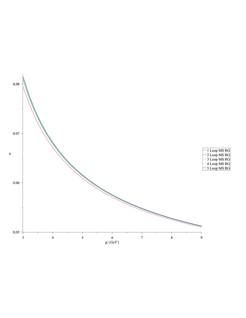
In Fig. 1 we plot the result of eq. (6a), cutting the infinite sum off at n = 0 , 1 , 2 , 3 𝑛 0 1 2 3
n=0,1,2,3 4 4 4 a ( M z ) = 0.1185 / π 𝑎 subscript 𝑀 𝑧 0.1185 𝜋 a(M_{z})=0.1185/\pi n f = 5 subscript 𝑛 𝑓 5 n_{f}=5
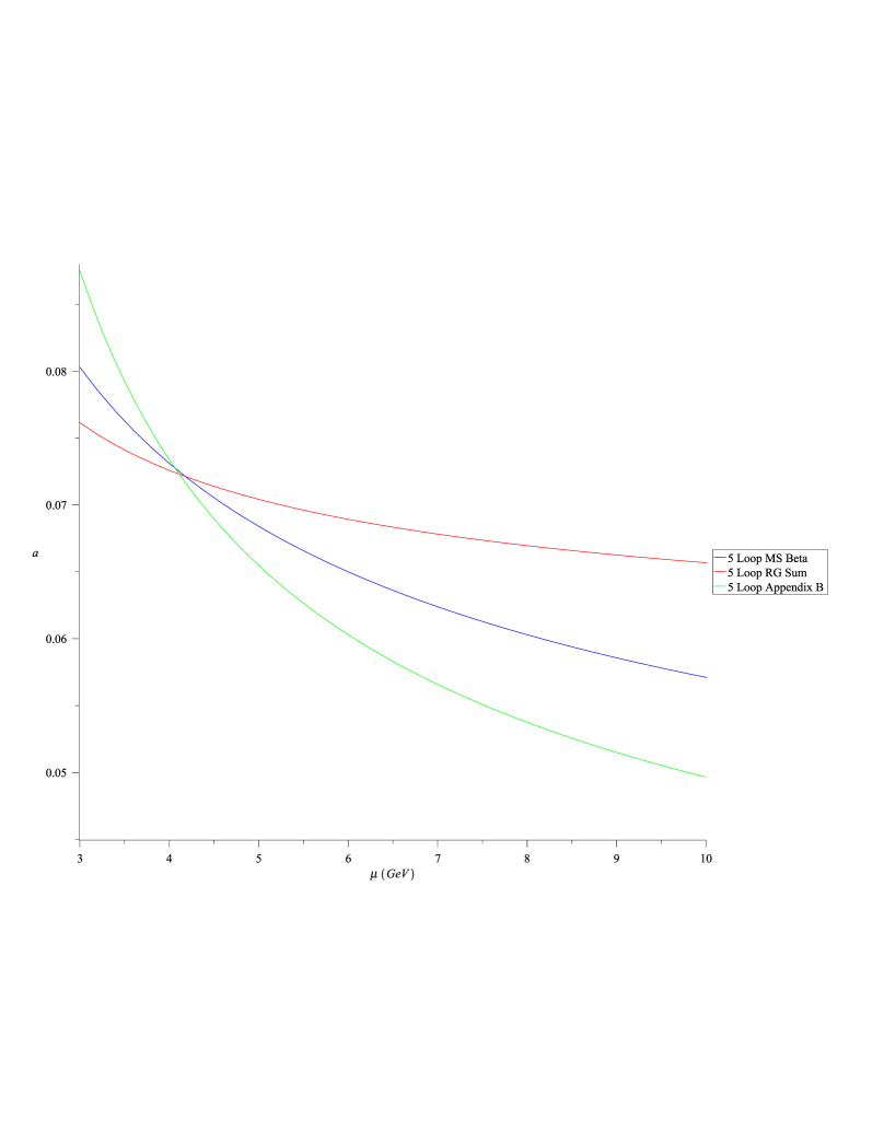
The three curves in Fig. 2 present results from three different ways of obtaining a ( μ ) 𝑎 𝜇 a(\mu) b , c , c 2 , c 3 𝑏 𝑐 subscript 𝑐 2 subscript 𝑐 3
b,c,c_{2},c_{3} c 4 subscript 𝑐 4 c_{4} n = 4 𝑛 4 n=4 a ( m b = 4.18 G e V ) = 0.072121836 𝑎 subscript 𝑚 𝑏 4.18 𝐺 𝑒 𝑉 0.072121836 a(m_{b}=4.18GeV)=0.072121836 β ( a ) 𝛽 𝑎 \beta(a) M S ¯ ¯ 𝑀 𝑆 \overline{MS} Λ Q C D subscript Λ 𝑄 𝐶 𝐷 \Lambda_{QCD} L 𝐿 L n f = 5 subscript 𝑛 𝑓 5 n_{f}=5 a ( m b = 4.18 G e V ) = 0.072121836 𝑎 subscript 𝑚 𝑏 4.18 𝐺 𝑒 𝑉 0.072121836 a(m_{b}=4.18GeV)=0.072121836 μ 𝜇 \mu μ = m b 𝜇 subscript 𝑚 𝑏 \mu=m_{b} μ 𝜇 \mu
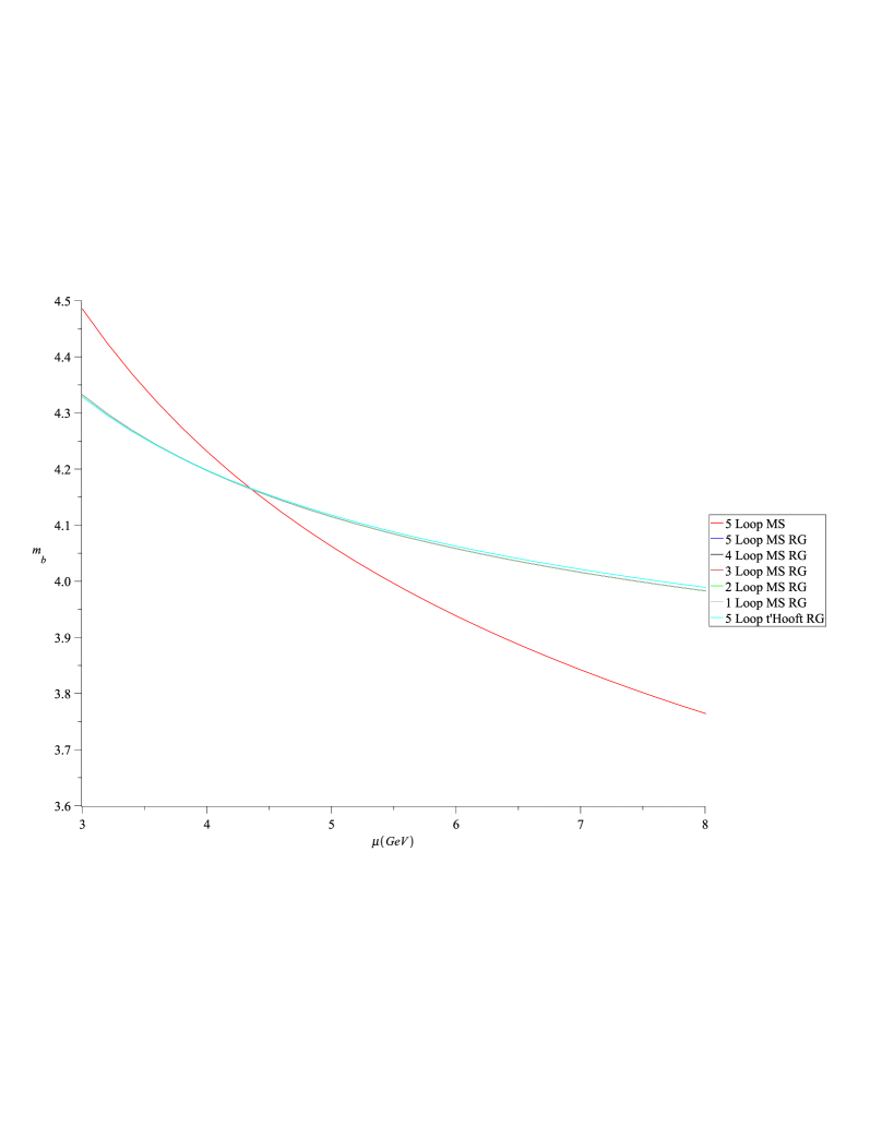
Curves for the running mass m ( μ ) 𝑚 𝜇 m(\mu) m b ( m b ) = 4.18 G e V subscript 𝑚 𝑏 subscript 𝑚 𝑏 4.18 𝐺 𝑒 𝑉 m_{b}(m_{b})=4.18GeV n = 0 , 1 , 2 , 3 𝑛 0 1 2 3
n=0,1,2,3 4 4 4 μ 𝜇 \mu
When examining a perturbative evaluation of a physical process using the functional dependence of the running coupling and running mass on the mass scale, it is apparent from our figures that using the RG summed results developed in our paper are to be preferred. In Fig. 1 we see that RG summation, by virtue of the fact that it includes contributions from all orders of perturbation theory, is relatively insensitive to inclusion of higher loop effects. We also see that ignoring the effects of higher orders, even when working with the five loop beta function, leads to distinct values of the running coupling. Fig. 2 shows that RG summation leads to a distinct value for the running coupling at high mass scale; it differs not only from what comes from direct integration of the defining equation for the running coupling, but also from the result of using the usual approach to obtaining the running coupling outlined in appendix B. This improvement is clearly the consequence of incorporating the contribution of higher loop effects through use of RG summation. Finally, Fig. 3 shows how RG summation of higher loop effects into the dependence of the running mass on the renormalization mass scale leads to results that are distinct from simply using the five loop result for the anomalous mass dimension and that these RG summed results are not greatly affected by higher loop contributions. To further substantiate these present findings, we are investigating distinct physical processes in an upcoming work [18].
Acknowledgements
R. Macleod had a helpful comment.
References
[1]
S. Weinberg, Phys. Rev. D8 , 3497 (1973).
[2]
G. ’t Hooft, Nucl. Phys. B61 , 455 (1973).
[3]
A. Deur, S.J. Brodsky, and G.F. de Teramond, Prog. Part. Nucl. Phys. 90 , 1 (2016).
[4]
A.L. Kataev, S.V. Mikhailov JHEP 1611 , 079 (2016);
X.G. Wu, S.J. Brodsky, and M. Mojaza, Prog. Part. Nucl. Phys. 72 , 44 (2013);
Phys. Rev. B655 , 221 (2003);
Phys. Rev. D60 , 105001 (1999).
[5]
P.M. Stevenson, Ann. of Phys. (N.Y.) 132 , 383 (1999).
[6]
F.A. Chishtie, D.G.C. McKeon and T.N. Sherry, (hep-th 1708.04219v2).
[7]
P.M. Stevenson, Phys. Rev. D23 , 2916 (1981).
[8]
D.G.C. McKeon, Can. J. Phys. 61 , 564 (1983); 59 , 1327 (1981).
[9]
D.G.C. McKeon, Phys. Rev. D92 , 045031 (2015).
[10]
F.A. Chishtie, M.D. LePage, D.G.C. McKeon, T.G. Steele and I. Zakout, Can. J. Phys. 86 , 1067 (2008).
[11]
T. Luthe, A. Maier, P. Marquard and Y. Schroder, JHEP 01 (2017) 081.
[12]
P.A. Baikov, K.G. Chetyrkin and J.H. Kuhn, Phys. Rev. Lett. 118 , 082002 (2017).
[13]
“Renormalization” J. Collins (Cambridge U. Press, Cambridge 1984).
[14]
K.G. Chetyrkin, B.A. Kniehl and M. Steinhauser, Phys. Rev. Lett. 79 , 2184 (1997).
[15]
G.M. Prosperi, M. Raciti and C. Simolo, Prog. Part. Nucl. Phys. 58 , 387 (2007).
[16]
D.G.C. McKeon and C.Z. Zhao, Nucl. Phys. B932 , 425 (2018).
[17]
G. ’t Hooft, “The Whys of Sub-Nuclear Physics,” Erice, 1977, ed. A. Zichichi, Plenum Press, N.Y. (1979).
[18]
F.A. Chishtie, D.G.C. McKeon and T.N. Sherry (in preparation).
Appendix A
The full solutions for T 3 subscript 𝑇 3 T_{3} T 4 subscript 𝑇 4 T_{4}
T 3 = 1 6 ρ w ρ − 3 [ C 3 , 0 ln 3 w + ( C 2 , 1 w + C 2 , 0 ) ln 2 w + ( C 1 , 2 w 2 + C 1 , 1 w + C 1 , 0 ) ln w \displaystyle T_{3}=\frac{1}{6}\rho\,{w}^{\rho-3}[C_{{3,0}}\ln^{3}w+\left(C_{{2,1}}w+C_{{2,0}}\right)\ln^{2}w+\left(C_{{1,2}}{w}^{2}+C_{{1,1}}w+C_{{1,0}}\right)\ln w
+ C 0 , 3 w 3 + C 0 , 2 w 2 + C 0 , 1 w + C 0 , 0 ] \displaystyle+C_{{0,3}}{w}^{3}+C_{{0,2}}{w}^{2}+C_{{0,1}}w+C_{{0,0}}] (A.1)
T 4 = 1 24 ρ w ρ − 4 [ D 4 , 0 ln 4 w + ( D 3 , 1 w + D 3 , 0 ) ln 3 w + ( D 2 , 2 w 2 + D 2 , 1 w + D 2 , 0 ) ln 2 w \displaystyle T_{{4}}=\frac{1}{24}\rho\,{w}^{\rho-4}[D_{{4,0}}\ln^{4}w+\left(D_{{3,1}}w+D_{{3,0}}\right)\ln^{3}w+(D_{{2,2}}{w}^{2}+D_{{2,1}}w+D_{{2,0}})\ln^{2}w
+ ( D 1 , 3 w 3 + D 1 , 2 w 2 + D 1 , 1 w + D 1 , 0 ) ln w + D 0 , 4 w 4 + D 0 , 3 w 3 + D 0 , 2 w 2 + D 0 , 1 w + D 0 , 0 ] \displaystyle+(D_{{1,3}}{w}^{3}+D_{{1,2}}{w}^{2}+D_{{1,1}}w+D_{{1,0}})\ln w+D_{{0,4}}{w}^{4}+D_{{0,3}}{w}^{3}+D_{{0,2}}{w}^{2}+D_{{0,1}}w+D_{{0,0}}] (A.2)
where the associated coefficients for T 3 subscript 𝑇 3 T_{3}
C 0 , 0 = ( c − g 1 ) 3 ρ 2 + ( 3 c − 3 g 1 ) ( c 2 + c g 1 − c 2 − g 2 ) ρ − c 3 + 4 c 2 g 1 + ( 2 c 2 + 2 g 2 ) c − 4 c 2 g 1 − c 3 − 2 g 3 subscript 𝐶 0 0
superscript 𝑐 subscript 𝑔 1 3 superscript 𝜌 2 3 𝑐 3 subscript 𝑔 1 superscript 𝑐 2 𝑐 subscript 𝑔 1 subscript 𝑐 2 subscript 𝑔 2 𝜌 superscript 𝑐 3 4 superscript 𝑐 2 subscript 𝑔 1 2 subscript 𝑐 2 2 subscript 𝑔 2 𝑐 4 subscript 𝑐 2 subscript 𝑔 1 subscript 𝑐 3 2 subscript 𝑔 3 C_{{0,0}}=\left(c-g_{{1}}\right)^{3}{\rho}^{2}+\left(3\,c-3\,g_{{1}}\right)\left({c}^{2}+cg_{{1}}-c_{{2}}-g_{{2}}\right)\rho-{c}^{3}+4\,{c}^{2}g_{{1}}+\left(2\,c_{{2}}+2\,g_{{2}}\right)c-4\,c_{{2}}g_{{1}}-c_{{3}}-2\,g_{{3}} (A.3)
C 0 , 1 = − 3 ( c − g 1 ) 3 ρ 2 − ( 3 c − 3 g 1 ) ( 3 c 2 + c g 1 − 3 c 2 − g 2 ) ρ − 6 c 2 g 1 + 6 c 2 g 1 subscript 𝐶 0 1
3 superscript 𝑐 subscript 𝑔 1 3 superscript 𝜌 2 3 𝑐 3 subscript 𝑔 1 3 superscript 𝑐 2 𝑐 subscript 𝑔 1 3 subscript 𝑐 2 subscript 𝑔 2 𝜌 6 superscript 𝑐 2 subscript 𝑔 1 6 subscript 𝑐 2 subscript 𝑔 1 C_{{0,1}}=-3\,\left(c-g_{{1}}\right)^{3}{\rho}^{2}-\left(3\,c-3\,g_{{1}}\right)\left(3\,{c}^{2}+cg_{{1}}-3\,c_{{2}}-g_{{2}}\right)\rho-6\,{c}^{2}g_{{1}}+6\,c_{{2}}g_{{1}} (A.4)
C 0 , 2 = 3 ( c − g 1 ) 3 ρ 2 + ( 3 c − 3 g 1 ) ( 3 c 2 − c g 1 − 3 c 2 + g 2 ) ρ + 3 c 3 − 6 c c 2 + 3 c 3 subscript 𝐶 0 2
3 superscript 𝑐 subscript 𝑔 1 3 superscript 𝜌 2 3 𝑐 3 subscript 𝑔 1 3 superscript 𝑐 2 𝑐 subscript 𝑔 1 3 subscript 𝑐 2 subscript 𝑔 2 𝜌 3 superscript 𝑐 3 6 𝑐 subscript 𝑐 2 3 subscript 𝑐 3 C_{{0,2}}=3\,\left(c-g_{{1}}\right)^{3}{\rho}^{2}+\left(3\,c-3\,g_{{1}}\right)\left(3\,{c}^{2}-cg_{{1}}-3\,c_{{2}}+g_{{2}}\right)\rho+3\,{c}^{3}-6\,cc_{{2}}+3\,c_{{3}} (A.5)
C 0 , 3 = − ( c − g 1 ) 3 ρ 2 − ( 3 c − 3 g 1 ) ( c 2 − c g 1 − c 2 + g 2 ) ρ − 2 c 3 + 2 c 2 g 1 + ( 4 c 2 − 2 g 2 ) c − 2 c 2 g 1 − 2 c 3 + 2 g 3 subscript 𝐶 0 3
superscript 𝑐 subscript 𝑔 1 3 superscript 𝜌 2 3 𝑐 3 subscript 𝑔 1 superscript 𝑐 2 𝑐 subscript 𝑔 1 subscript 𝑐 2 subscript 𝑔 2 𝜌 2 superscript 𝑐 3 2 superscript 𝑐 2 subscript 𝑔 1 4 subscript 𝑐 2 2 subscript 𝑔 2 𝑐 2 subscript 𝑐 2 subscript 𝑔 1 2 subscript 𝑐 3 2 subscript 𝑔 3 C_{{0,3}}=-\left(c-g_{{1}}\right)^{3}{\rho}^{2}-\left(3\,c-3\,g_{{1}}\right)\left({c}^{2}-cg_{{1}}-c_{{2}}+g_{{2}}\right)\rho-2\,{c}^{3}+2\,{c}^{2}g_{{1}}+\left(4\,c_{{2}}-2\,g_{{2}}\right)c-2\,c_{{2}}g_{{1}}-2\,c_{{3}}+2\,g_{{3}} (A.6)
C 1 , 0 = 3 c [ ( c − g 1 ) 2 ρ 2 + ( c 2 + 3 c g 1 − 2 g 1 2 − c 2 − g 2 ) ρ − 2 c 2 + 2 c 2 + 2 g 2 ] subscript 𝐶 1 0
3 𝑐 delimited-[] superscript 𝑐 subscript 𝑔 1 2 superscript 𝜌 2 superscript 𝑐 2 3 𝑐 subscript 𝑔 1 2 superscript subscript 𝑔 1 2 subscript 𝑐 2 subscript 𝑔 2 𝜌 2 superscript 𝑐 2 2 subscript 𝑐 2 2 subscript 𝑔 2 C_{{1,0}}=3\,c\left[\left(c-g_{{1}}\right)^{2}{\rho}^{2}+\left({c}^{2}+3\,cg_{{1}}-2\,{g_{{1}}}^{2}-c_{{2}}-g_{{2}}\right)\rho-2\,{c}^{2}+2\,c_{{2}}+2\,g_{{2}}\right] (A.7)
C 1 , 1 = − 6 c [ ( c − g 1 ) 2 ρ 2 + ( c 2 + c g 1 − g 1 2 − c 2 ) ρ − c 2 + c 2 ] subscript 𝐶 1 1
6 𝑐 delimited-[] superscript 𝑐 subscript 𝑔 1 2 superscript 𝜌 2 superscript 𝑐 2 𝑐 subscript 𝑔 1 superscript subscript 𝑔 1 2 subscript 𝑐 2 𝜌 superscript 𝑐 2 subscript 𝑐 2 C_{{1,1}}=-6\,c\left[\left(c-g_{{1}}\right)^{2}{\rho}^{2}+\left({c}^{2}+cg_{{1}}-{g_{{1}}}^{2}-c_{{2}}\right)\rho-{c}^{2}+c_{{2}}\right] (A.8)
C 1 , 2 = 3 c [ ( c − g 1 ) 2 ρ 2 + ( c 2 − c g 1 − c 2 + g 2 ) ρ ] subscript 𝐶 1 2
3 𝑐 delimited-[] superscript 𝑐 subscript 𝑔 1 2 superscript 𝜌 2 superscript 𝑐 2 𝑐 subscript 𝑔 1 subscript 𝑐 2 subscript 𝑔 2 𝜌 C_{{1,2}}=3\,c\left[\left(c-g_{{1}}\right)^{2}{\rho}^{2}+\left({c}^{2}-cg_{{1}}-c_{{2}}+g_{{2}}\right)\rho\right] (A.8)
C 2 , 0 = 3 c 2 [ ( c − g 1 ) ρ 2 + ( − c + 3 g 1 ) ρ − c − 2 g 1 ] subscript 𝐶 2 0
3 superscript 𝑐 2 delimited-[] 𝑐 subscript 𝑔 1 superscript 𝜌 2 𝑐 3 subscript 𝑔 1 𝜌 𝑐 2 subscript 𝑔 1 C_{{2,0}}=3\,{c}^{2}\left[\left(c-g_{{1}}\right){\rho}^{2}+\left(-c+3\,g_{{1}}\right)\rho-c-2\,g_{{1}}\right] (A.9)
C 2 , 1 = − 3 ρ c 2 ( ρ − 1 ) ( c − g 1 ) subscript 𝐶 2 1
3 𝜌 superscript 𝑐 2 𝜌 1 𝑐 subscript 𝑔 1 C_{{2,1}}=-3\,\rho\,{c}^{2}\left(\rho-1\right)\left(c-g_{{1}}\right) (A.10)
C 3 , 0 = c 3 ( ρ − 1 ) ( ρ − 2 ) subscript 𝐶 3 0
superscript 𝑐 3 𝜌 1 𝜌 2 C_{{3,0}}={c}^{3}\left(\rho-1\right)\left(\rho-2\right) (A.11)
.
The coefficients for the T 4 subscript 𝑇 4 T_{4}
D 0 , 0 = ρ 3 ( c − g 1 ) 4 + 6 ρ 2 ( c − g 1 ) 2 ( c 2 + c g 1 − c 2 − g 2 ) + ρ ( − c 4 + 26 c 3 g 1 + ( − 13 g 1 2 + 2 c 2 + 2 g 2 ) c 2 \displaystyle D_{{0,0}}={\rho}^{3}(c-g_{{1}})^{4}+6\,{\rho}^{2}(c-g_{{1}})^{2}({c}^{2}+cg_{{1}}-c_{{2}}-g_{{2}})+\rho\,(-{c}^{4}+26\,{c}^{3}g_{{1}}+(-13\,{g_{{1}}}^{2}+2\,c_{{2}}+2\,g_{{2}}){c}^{2}
+ ( − 30 c 2 g 1 − 14 g 1 g 2 − 4 c 3 − 8 g 3 ) c + 3 c 2 2 + ( 16 g 1 2 + 6 g 2 ) c 2 + 4 c 3 g 1 + 8 g 1 g 3 + 3 g 2 2 ) − 10 c 4 − 6 c 3 g 1 \displaystyle+(-30\,c_{{2}}g_{{1}}-14\,g_{{1}}g_{{2}}-4\,c_{{3}}-8\,g_{{3}})c+3\,{c_{{2}}}^{2}+(16\,{g_{{1}}}^{2}+6\,g_{{2}})c_{{2}}+4\,c_{{3}}g_{{1}}+8\,g_{{1}}g_{{3}}+3\,{g_{{2}}}^{2})-10\,{c}^{4}-6\,{c}^{3}g_{{1}}
+ ( 18 c 2 + 18 g 2 ) c 2 + ( 12 c 2 g 1 + 4 c 3 + 6 g 3 ) c − 10 c 2 2 − 18 c 2 g 2 − 6 c 3 g 1 − 2 c 4 − 6 g 4 18 subscript 𝑐 2 18 subscript 𝑔 2 superscript 𝑐 2 12 subscript 𝑐 2 subscript 𝑔 1 4 subscript 𝑐 3 6 subscript 𝑔 3 𝑐 10 superscript subscript 𝑐 2 2 18 subscript 𝑐 2 subscript 𝑔 2 6 subscript 𝑐 3 subscript 𝑔 1 2 subscript 𝑐 4 6 subscript 𝑔 4 \displaystyle+(18\,c_{{2}}+18\,g_{{2}}){c}^{2}+(12\,c_{{2}}g_{{1}}+4\,c_{{3}}+6\,g_{{3}})c-10\,{c_{{2}}}^{2}-18\,c_{{2}}g_{{2}}-6\,c_{{3}}g_{{1}}-2\,c_{{4}}-6\,g_{{4}} (A.12)
D 0 , 1 = − 4 ρ 3 ( c − g 1 ) 4 − 12 ρ 2 ( c − g 1 ) 2 ( 2 c 2 + c g 1 − 2 c 2 − g 2 ) + ρ ( − 8 c 4 − 56 c 3 g 1 + ( 40 g 1 2 + 16 c 2 + 4 g 2 ) c 2 \displaystyle D_{{0,1}}=-4\,{\rho}^{3}(c-g_{{1}})^{4}-12\,{\rho}^{2}(c-g_{{1}})^{2}(2\,{c}^{2}+cg_{{1}}-2\,c_{{2}}-g_{{2}})+\rho\,(-8\,{c}^{4}-56\,{c}^{3}g_{{1}}+(40\,{g_{{1}}}^{2}+16\,c_{{2}}+4\,g_{{2}}){c}^{2}
+ ( 60 c 2 g 1 + 8 g 1 g 2 + 4 c 3 + 8 g 3 ) c − 12 c 2 2 + ( − 40 g 1 2 − 12 g 2 ) c 2 − 4 c 3 g 1 − 8 g 1 g 3 ) \displaystyle+(60\,c_{{2}}g_{{1}}+8\,g_{{1}}g_{{2}}+4\,c_{{3}}+8\,g_{{3}})c-12\,{c_{{2}}}^{2}+(-40\,{g_{{1}}}^{2}-12\,g_{{2}})c_{{2}}-4\,c_{{3}}g_{{1}}-8\,g_{{1}}g_{{3}})
+ ( 24 c 2 − 24 c 2 ) ( c 2 − c 2 − g 2 ) 24 superscript 𝑐 2 24 subscript 𝑐 2 superscript 𝑐 2 subscript 𝑐 2 subscript 𝑔 2 \displaystyle+(24\,{c}^{2}-24\,c_{{2}})({c}^{2}-c_{{2}}-g_{{2}}) (A.13)
D 0 , 2 = 6 ρ 3 ( c − g 1 ) 4 + 36 ρ 2 ( c − g 1 ) 2 ( c 2 − c 2 ) + ρ ( 30 c 4 + 12 c 3 g 1 + ( − 30 g 1 2 − 60 c 2 ) c 2 + ( 12 g 1 g 2 + 12 c 3 ) c \displaystyle D_{{0,2}}=6\,{\rho}^{3}(c-g_{{1}})^{4}+36\,{\rho}^{2}\left(c-g_{{1}}\right)^{2}\left({c}^{2}-c_{{2}}\right)+\rho\,(30\,{c}^{4}+12\,{c}^{3}g_{{1}}+\left(-30\,{g_{{1}}}^{2}-60\,c_{{2}}\right){c}^{2}+\left(12\,g_{{1}}g_{{2}}+12\,c_{{3}}\right)c
+ 24 c 2 g 1 2 + 18 c 2 2 − 12 c 3 g 1 − 6 g 2 2 ) − 12 c 4 + 12 c 3 g 1 + 24 c 2 c 2 − 24 c c 2 g 1 − 12 c 2 2 + 12 c 3 g 1 \displaystyle+24\,c_{{2}}{g_{{1}}}^{2}+18\,{c_{{2}}}^{2}-12\,c_{{3}}g_{{1}}-6\,{g_{{2}}}^{2})-12\,{c}^{4}+12\,{c}^{3}g_{{1}}+24\,{c}^{2}c_{{2}}-24\,cc_{{2}}g_{{1}}-12\,{c_{{2}}}^{2}+12\,c_{{3}}g_{{1}} (A.14)
D 0 , 3 = − 4 ρ 3 ( c − g 1 ) 4 − 12 ρ 2 ( c − g 1 ) 2 ( 2 c 2 − c g 1 − 2 c 2 + g 2 ) + ρ ( − 32 c 4 + 40 c 3 g 1 + ( − 8 g 1 2 + 64 c 2 \displaystyle D_{{0,3}}=-4\,{\rho}^{3}\left(c-g_{{1}}\right)^{4}-12\,{\rho}^{2}\left(c-g_{{1}}\right)^{2}\left(2\,{c}^{2}-cg_{{1}}-2\,c_{{2}}+g_{{2}}\right)+\rho\,(-32\,{c}^{4}+40\,{c}^{3}g_{{1}}+(-8\,{g_{{1}}}^{2}+64\,c_{{2}}
− 20 g 2 ) c 2 + ( − 60 c 2 g 1 + 8 g 1 g 2 − 20 c 3 + 8 g 3 ) c − 12 c 2 2 + ( 8 g 1 2 + 12 g 2 ) c 2 + 20 c 3 g 1 − 8 g 1 g 3 ) \displaystyle-20\,g_{{2}}){c}^{2}+(-60\,c_{{2}}g_{{1}}+8\,g_{{1}}g_{{2}}-20\,c_{{3}}+8\,g_{{3}})c-12\,{c_{{2}}}^{2}+\left(8\,{g_{{1}}}^{2}+12\,g_{{2}}\right)c_{{2}}+20\,c_{{3}}g_{{1}}-8\,g_{{1}}g_{{3}})
− 8 c 4 + 24 c 2 c 2 − 16 c c 3 − 8 c 2 2 + 8 c 4 8 superscript 𝑐 4 24 superscript 𝑐 2 subscript 𝑐 2 16 𝑐 subscript 𝑐 3 8 superscript subscript 𝑐 2 2 8 subscript 𝑐 4 \displaystyle-8\,{c}^{4}+24\,{c}^{2}c_{{2}}-16\,cc_{{3}}-8\,{c_{{2}}}^{2}+8\,c_{{4}} (A.15)
D 0 , 4 = ρ 3 ( c − g 1 ) 4 + 6 ρ 2 ( c − g 1 ) 2 ( c 2 − c g 1 − c 2 + g 2 ) + ρ ( 11 c 4 − 22 c 3 g 1 + ( 11 g 1 2 − 22 c 2 + 14 g 2 ) c 2 \displaystyle D_{{0,4}}={\rho}^{3}\left(c-g_{{1}}\right)^{4}+6\,{\rho}^{2}\left(c-g_{{1}}\right)^{2}\left({c}^{2}-cg_{{1}}-c_{{2}}+g_{{2}}\right)+\rho\,(11\,{c}^{4}-22\,{c}^{3}g_{{1}}+\left(11\,{g_{{1}}}^{2}-22\,c_{{2}}+14\,g_{{2}}\right){c}^{2}
+ ( 30 c 2 g 1 − 14 g 1 g 2 + 8 c 3 − 8 g 3 ) c − 8 c 2 g 1 2 + 3 c 2 2 − 6 c 2 g 2 − 8 c 3 g 1 + 8 g 1 g 3 + 3 g 2 2 ) + 6 c 4 − 6 c 3 g 1 \displaystyle+\left(30\,c_{{2}}g_{{1}}-14\,g_{{1}}g_{{2}}+8\,c_{{3}}-8\,g_{{3}}\right)c-8\,c_{{2}}{g_{{1}}}^{2}+3\,{c_{{2}}}^{2}-6\,c_{{2}}g_{{2}}-8\,c_{{3}}g_{{1}}+8\,g_{{1}}g_{{3}}+3\,{g_{{2}}}^{2})+6\,{c}^{4}-6\,{c}^{3}g_{{1}}
+ ( − 18 c 2 + 6 g 2 ) c 2 + ( 12 c 2 g 1 + 12 c 3 − 6 g 3 ) c + 6 c 2 2 − 6 c 2 g 2 − 6 c 3 g 1 − 6 c 4 + 6 g 4 18 subscript 𝑐 2 6 subscript 𝑔 2 superscript 𝑐 2 12 subscript 𝑐 2 subscript 𝑔 1 12 subscript 𝑐 3 6 subscript 𝑔 3 𝑐 6 superscript subscript 𝑐 2 2 6 subscript 𝑐 2 subscript 𝑔 2 6 subscript 𝑐 3 subscript 𝑔 1 6 subscript 𝑐 4 6 subscript 𝑔 4 \displaystyle+\left(-18\,c_{{2}}+6\,g_{{2}}\right){c}^{2}+\left(12\,c_{{2}}g_{{1}}+12\,c_{{3}}-6\,g_{{3}}\right)c+6\,{c_{{2}}}^{2}-6\,c_{{2}}g_{{2}}-6\,c_{{3}}g_{{1}}-6\,c_{{4}}+6\,g_{{4}} (A.16)
D 1 , 0 = 4 c [ ( c − g 1 ) 3 ρ 3 + ( 3 c − 3 g 1 ) ( c 2 + 2 c g 1 − g 1 2 − c 2 − g 2 ) ρ 2 + ( − 7 c 3 + 13 c 2 g 1 \displaystyle D_{{1,0}}=4\,c[\left(c-g_{{1}}\right)^{3}{\rho}^{3}+\left(3\,c-3\,g_{{1}}\right)\left({c}^{2}+2\,cg_{{1}}-{g_{{1}}}^{2}-c_{{2}}-g_{{2}}\right){\rho}^{2}+(-7\,{c}^{3}+13\,{c}^{2}g_{{1}}
+ ( 3 g 1 2 + 8 c 2 + 8 g 2 ) c − 13 c 2 g 1 − 9 g 1 g 2 − c 3 − 2 g 3 ) ρ − 3 c 3 − 12 c 2 g 1 + 12 c 2 g 1 + 3 c 3 + 6 g 3 ] \displaystyle+\left(3\,{g_{{1}}}^{2}+8\,c_{{2}}+8\,g_{{2}}\right)c-13\,c_{{2}}g_{{1}}-9\,g_{{1}}g_{{2}}-c_{{3}}-2\,g_{{3}})\rho-3\,{c}^{3}-12\,{c}^{2}g_{{1}}+12\,c_{{2}}g_{{1}}+3\,c_{{3}}+6\,g_{{3}}] (A.17)
D 1 , 1 = − 12 c [ ( c − g 1 ) 3 ρ 3 + ( c − g 1 ) ( 3 c 2 + 3 c g 1 − 2 g 1 2 − 3 c 2 − g 2 ) ρ 2 + ( − 4 c 3 + 8 c 2 g 1 + 4 c c 2 + 2 c g 2 \displaystyle D_{{1,1}}=-12\,c[\left(c-g_{{1}}\right)^{3}{\rho}^{3}+\left(c-g_{{1}}\right)\left(3\,{c}^{2}+3\,cg_{{1}}-2\,{g_{{1}}}^{2}-3\,c_{{2}}-g_{{2}}\right){\rho}^{2}+(-4\,{c}^{3}+8\,{c}^{2}g_{{1}}+4\,cc_{{2}}+2\,cg_{{2}}
− 8 c 2 g 1 − 2 g 1 g 2 ) ρ − 2 c 3 − 4 c 2 g 1 + 2 c c 2 + 4 c 2 g 1 ] \displaystyle-8\,c_{{2}}g_{{1}}-2\,g_{{1}}g_{{2}})\rho-2\,{c}^{3}-4\,{c}^{2}g_{{1}}+2\,cc_{{2}}+4\,c_{{2}}g_{{1}}] (A.18)
D 1 , 2 = 12 c [ ( c − g 1 ) 3 ρ 3 + ( c − g 1 ) ( 3 c 2 − g 1 2 − 3 c 2 + g 2 ) ρ 2 + ( − c 3 + 3 c 2 g 1 − c g 1 2 − 3 c 2 g 1 \displaystyle D_{{1,2}}=12\,c[\left(c-g_{{1}}\right)^{3}{\rho}^{3}+\left(c-g_{{1}}\right)\left(3\,{c}^{2}-{g_{{1}}}^{2}-3\,c_{{2}}+g_{{2}}\right){\rho}^{2}+(-{c}^{3}+3\,{c}^{2}g_{{1}}-c{g_{{1}}}^{2}-3\,c_{{2}}g_{{1}}
+ g 1 g 2 + c 3 ) ρ − c 3 + 2 c c 2 − c 3 ] \displaystyle+g_{{1}}g_{{2}}+c_{{3}})\rho-{c}^{3}+2\,cc_{{2}}-c_{{3}}] (A.19)
D 1 , 3 = − 4 c ρ [ ( c − g 1 ) 3 ρ 2 + ( 3 c − 3 g 1 ) ( c 2 − c g 1 − c 2 + g 2 ) ρ + 2 c 3 − 2 c 2 g 1 + ( − 4 c 2 + 2 g 2 ) c \displaystyle D_{{1,3}}=-4\,c\rho\,[\left(c-g_{{1}}\right)^{3}{\rho}^{2}+\left(3\,c-3\,g_{{1}}\right)\left({c}^{2}-cg_{{1}}-c_{{2}}+g_{{2}}\right)\rho+2\,{c}^{3}-2\,{c}^{2}g_{{1}}+\left(-4\,c_{{2}}+2\,g_{{2}}\right)c
+ 2 c 2 g 1 + 2 c 3 − 2 g 3 ] \displaystyle+2\,c_{{2}}g_{{1}}+2\,c_{{3}}-2\,g_{{3}}] (A.20)
D 2 , 0 = 6 c 2 [ ( c − g 1 ) 2 ρ 3 + ( 7 c g 1 − 5 g 1 2 − c 2 − g 2 ) ρ 2 + ( − 7 c 2 − 3 c g 1 + 6 g 1 2 + 5 c 2 + 5 g 2 ) ρ \displaystyle D_{{2,0}}=6\,{c}^{2}[\left(c-g_{{1}}\right)^{2}{\rho}^{3}+\left(7\,cg_{{1}}-5\,{g_{{1}}}^{2}-c_{{2}}-g_{{2}}\right){\rho}^{2}+(-7\,{c}^{2}-3\,cg_{{1}}+6\,{g_{{1}}}^{2}+5\,c_{{2}}+5\,g_{{2}})\rho
+ 4 c 2 − 4 c g 1 − 6 c 2 − 6 g 2 ] \displaystyle+4\,{c}^{2}-4\,cg_{{1}}-6\,c_{{2}}-6\,g_{{2}}] (A.21)
D 2 , 1 = − 12 c 2 ( ( c − g 1 ) 2 ρ 3 + ( 4 c g 1 − 3 g 1 2 − c 2 ) ρ 2 + ( − 4 c 2 − c g 1 + 2 g 1 2 + 3 c 2 ) ρ + 2 c 2 − 2 c 2 ) subscript 𝐷 2 1
12 superscript 𝑐 2 superscript 𝑐 subscript 𝑔 1 2 superscript 𝜌 3 4 𝑐 subscript 𝑔 1 3 superscript subscript 𝑔 1 2 subscript 𝑐 2 superscript 𝜌 2 4 superscript 𝑐 2 𝑐 subscript 𝑔 1 2 superscript subscript 𝑔 1 2 3 subscript 𝑐 2 𝜌 2 superscript 𝑐 2 2 subscript 𝑐 2 \displaystyle D_{{2,1}}=-12\,{c}^{2}\left(\left(c-g_{{1}}\right)^{2}{\rho}^{3}+\left(4\,cg_{{1}}-3\,{g_{{1}}}^{2}-c_{{2}}\right){\rho}^{2}+\left(-4\,{c}^{2}-cg_{{1}}+2\,{g_{{1}}}^{2}+3\,c_{{2}}\right)\rho+2\,{c}^{2}-2\,c_{{2}}\right) (A.22)
D 2 , 2 = 6 c 2 ρ ( ρ − 1 ) ( ( c − g 1 ) 2 ρ + c ( c − g 1 ) − c 2 + g 2 ) subscript 𝐷 2 2
6 superscript 𝑐 2 𝜌 𝜌 1 superscript 𝑐 subscript 𝑔 1 2 𝜌 𝑐 𝑐 subscript 𝑔 1 subscript 𝑐 2 subscript 𝑔 2 \displaystyle D_{{2,2}}=6\,{c}^{2}\rho\,\left(\rho-1\right)\left(\left(c-g_{{1}}\right)^{2}\rho+c\left(c-g_{{1}}\right)-c_{{2}}+g_{{2}}\right) (A.23)
D 3 , 0 = 4 c 3 ( ( c − g 1 ) ρ 3 + ( − 3 c + 6 g 1 ) ρ 2 + ( − c − 11 g 1 ) ρ + 5 c + 6 g 1 ) subscript 𝐷 3 0
4 superscript 𝑐 3 𝑐 subscript 𝑔 1 superscript 𝜌 3 3 𝑐 6 subscript 𝑔 1 superscript 𝜌 2 𝑐 11 subscript 𝑔 1 𝜌 5 𝑐 6 subscript 𝑔 1 \displaystyle D_{{3,0}}=4\,{c}^{3}\left(\left(c-g_{{1}}\right){\rho}^{3}+\left(-3\,c+6\,g_{{1}}\right){\rho}^{2}+\left(-c-11\,g_{{1}}\right)\rho+5\,c+6\,g_{{1}}\right) (A.24)
D 3 , 1 = − 4 c 3 ρ ( ρ − 1 ) ( ρ − 2 ) ( c − g 1 ) subscript 𝐷 3 1
4 superscript 𝑐 3 𝜌 𝜌 1 𝜌 2 𝑐 subscript 𝑔 1 \displaystyle D_{{3,1}}=-4\,{c}^{3}\rho\,\left(\rho-1\right)\left(\rho-2\right)\left(c-g_{{1}}\right) (A.25)
D 4 , 0 = c 4 ( ρ − 1 ) ( ρ − 2 ) ( ρ − 3 ) subscript 𝐷 4 0
superscript 𝑐 4 𝜌 1 𝜌 2 𝜌 3 \displaystyle D_{{4,0}}={c}^{4}\left(\rho-1\right)\left(\rho-2\right)\left(\rho-3\right) (A.26)
Appendix B
The equation
a ( μ ′ ) = ∑ n = 0 ∞ S n ( a ℓ ) a n + 1 𝑎 superscript 𝜇 ′ superscript subscript 𝑛 0 subscript 𝑆 𝑛 𝑎 ℓ superscript 𝑎 𝑛 1 a(\mu^{\prime})=\sum_{n=0}^{\infty}S_{n}(a\ell)a^{n+1} (B.1)
which follows from eqs. (4a,6a) shows how a 𝑎 a a ( μ ) 𝑎 𝜇 a(\mu) a ( μ ′ ) 𝑎 superscript 𝜇 ′ a(\mu^{\prime}) a 𝑎 a
a ( μ ) = ∑ n = 1 ∞ ∑ m = 0 n − 1 x n m ln m L L n ( L ≡ ln μ Λ ) . 𝑎 𝜇 superscript subscript 𝑛 1 superscript subscript 𝑚 0 𝑛 1 subscript 𝑥 𝑛 𝑚 superscript 𝑚 𝐿 superscript 𝐿 𝑛 𝐿 𝜇 Λ
a(\mu)=\sum_{n=1}^{\infty}\sum_{m=0}^{n-1}\frac{x_{nm}\ln^{m}L}{L^{n}}\qquad\left(L\equiv\ln\frac{\mu}{\Lambda}\right). (B.2)
With β ( a ) 𝛽 𝑎 \beta(a) 1 L 2 1 superscript 𝐿 2 \frac{1}{L^{2}}
− x 10 = − b x 10 2 ⇒ x 10 = 1 / b . subscript 𝑥 10 𝑏 superscript subscript 𝑥 10 2 ⇒ subscript 𝑥 10 1 𝑏 -x_{10}=-bx_{10}^{2}\Rightarrow x_{10}=1/b. (B.3)
We find from higher order terms that
x 21 = − c b 2 − x 20 subscript 𝑥 21 𝑐 superscript 𝑏 2 subscript 𝑥 20 x_{21}=\frac{-c}{b^{2}}-x_{20} (B.4)
x 31 − x 30 = − b x 20 2 + 3 x 20 b − 3 c b x 20 − c 2 b 3 subscript 𝑥 31 subscript 𝑥 30 𝑏 superscript subscript 𝑥 20 2 3 subscript 𝑥 20 𝑏 3 𝑐 𝑏 subscript 𝑥 20 subscript 𝑐 2 superscript 𝑏 3 x_{31}-x_{30}=-bx_{20}^{2}+\frac{3x_{20}}{b}-\frac{3c}{b}x_{20}-\frac{c_{2}}{b^{3}} (B.5)
2 x 32 − 3 x 31 = 5 c x 20 b + 2 b x 20 2 − 2 x 31 + 3 c 2 b 3 2 subscript 𝑥 32 3 subscript 𝑥 31 5 𝑐 subscript 𝑥 20 𝑏 2 𝑏 superscript subscript 𝑥 20 2 2 subscript 𝑥 31 3 superscript 𝑐 2 superscript 𝑏 3 2x_{32}-3x_{31}=\frac{5cx_{20}}{b}+2bx_{20}^{2}-2x_{31}+\frac{3c^{2}}{b^{3}} (B.6)
3 x 32 = c 2 b 3 + 2 x 20 c b + b x 20 2 + 2 x 32 3 subscript 𝑥 32 superscript 𝑐 2 superscript 𝑏 3 2 subscript 𝑥 20 𝑐 𝑏 𝑏 superscript subscript 𝑥 20 2 2 subscript 𝑥 32 3x_{32}=\frac{c^{2}}{b^{3}}+\frac{2x_{20}c}{b}+bx_{20}^{2}+2x_{32} (B.7)
etc.
The boundary condition chosen in refs. [14,15] amounts to setting x 20 = 0 subscript 𝑥 20 0 x_{20}=0
a ( μ ) = 1 b L 𝑎 𝜇 1 𝑏 𝐿 \displaystyle a(\mu)=\frac{1}{bL} − c ln L b 2 L 2 + 1 b 3 L 3 [ c 2 ( ln 2 L − ln L − 1 ) + c 2 2 ] 𝑐 𝐿 superscript 𝑏 2 superscript 𝐿 2 1 superscript 𝑏 3 superscript 𝐿 3 delimited-[] superscript 𝑐 2 superscript 2 𝐿 𝐿 1 superscript subscript 𝑐 2 2 \displaystyle-\frac{c\ln L}{b^{2}L^{2}}+\frac{1}{b^{3}L^{3}}\left[c^{2}(\ln^{2}L-\ln L-1)+c_{2}^{2}\right] (B.8)
+ 1 b 4 L 4 [ c 3 ( − ln 3 L + 5 2 ln 2 L + 2 ln L − 1 2 ) − 3 c c 2 ln L + 1 2 c 3 ] 1 superscript 𝑏 4 superscript 𝐿 4 delimited-[] superscript 𝑐 3 superscript 3 𝐿 5 2 superscript 2 𝐿 2 𝐿 1 2 3 𝑐 subscript 𝑐 2 𝐿 1 2 subscript 𝑐 3 \displaystyle+\frac{1}{b^{4}L^{4}}\left[c^{3}\left(-\ln^{3}L+\frac{5}{2}\ln^{2}L+2\ln L-\frac{1}{2}\right)-3cc_{2}\ln L+\frac{1}{2}c_{3}\right]
+ 1 b 5 L 5 [ c 4 ( ln 4 L − 13 3 ln 3 L − 3 2 ln 2 L + 4 ln L + 7 6 ) \displaystyle+\frac{1}{b^{5}L^{5}}\Bigg{[}c^{4}\left(\ln^{4}L-\frac{13}{3}\ln^{3}L-\frac{3}{2}\ln^{2}L+4\ln L+\frac{7}{6}\right)
+ c 2 c 2 ( 6 ln 2 L − 3 ln L − 3 ) − c c 3 ( 2 ln L + 1 6 ) + 1 3 ( 5 c 2 2 + c 4 ) ] + … . \displaystyle+c^{2}c_{2}(6\ln^{2}L-3\ln L-3)-cc_{3}\left(2\ln L+\frac{1}{6}\right)+\frac{1}{3}(5c_{2}^{2}+c_{4})\Bigg{]}+\ldots.
This is quite distinct from eq. (B.1).
Figure 1: The μ 𝜇 \mu a 𝑎 a M S ¯ ¯ 𝑀 𝑆 {\overline{MS}} Figure 2: The μ 𝜇 \mu a 𝑎 a β 𝛽 \beta M S ¯ ¯ 𝑀 𝑆 {\overline{MS}} Figure 3: The μ 𝜇 \mu M S ¯ ¯ 𝑀 𝑆 {\overline{MS}} M S ¯ ¯ 𝑀 𝑆 {\overline{MS}}