UFIFT-QG-18-04

Cosmological Coleman-Weinberg Potentials and Inflation

J. H. Liao^1∗, S. P. Miao^1⋆ and R. P. Woodard^2†

¹ Department of Physics, National Cheng Kung University
No. 1, University Road, Tainan City 70101, TAIWAN

² Department of Physics, University of Florida,
Gainesville, FL 32611, UNITED STATES

ABSTRACT

We consider an additional fine-tuning problem which afflicts scalar-driven models of inflation. The problem is that successful reheating requires the inflaton be coupled to ordinary matter, and quantum fluctuations of this matter induces Coleman-Weinberg potentials which are not Planck-suppressed. Unlike the flat space case, these potentials depend upon a still-unknown, nonlocal functional of the metric which reduces to the Hubble parameter for de Sitter. Such a potential cannot be completely subtracted off by any local action. In a simple model we numerically consider one possible subtraction scheme in which the correction is locally subtracted at the beginning of inflation. For fermions the effect is to make the universe approach de Sitter with a smaller Hubble parameter. For gauge bosons the effect is to make inflation end almost instantly unless the gauge charge is unacceptably small.

PACS numbers: 04.50.Kd, 95.35.+d, 98.62.-g

^∗ e-mail: a0983028669@gmail.com

^⋆ e-mail: spmiao5@mail.ncku.edu.tw

^† e-mail: woodard@phys.ufl.edu

1 Introduction

The most recent results for the scalar spectral index $n_{s}$, and the limits on the tensor-to-scalar ratio $r$ [1], are still consistent with certain models of single scalar-driven inflation,

$$\mathcal{L}=\frac{R\sqrt{-g}}{16\pi G}-\frac{1}{2}\partial_{\mu}\varphi\partial_{\nu}\varphi g^{\mu\nu}\sqrt{-g}-V(\varphi)\sqrt{-g}\;.$$ (1)

However, the allowed models suffer from severe fine-tuning problems associated with the need to keep the potential very flat, with getting inflation to start and with avoiding the loss of predictivity through the formation of a multiverse [2]. This has led to much controversy within the inflation community [3, 4, 5].

The purpose of this paper is to study a different sort of fine-tuning problem which is associated with the necessity of coupling the inflaton to normal matter to make reheating efficient. It has long been known that the quantum fluctuations of such matter particles will induce Coleman-Weinberg corrections to the inflaton effective potential [6]. These corrections are dangerous for inflation because they are not Planck-suppressed [7].

Until recently the assumption was that cosmological Coleman-Weinberg potentials are simply local functions of the inflaton which could be subtracted at will. However, existing results (from scalars [8], from fermions [9, 10], and from gauge bosons [11, 12]) on de Sitter background show that the corrections actually take the form of the fourth power of the Hubble constant times a complicated function of the dimensionless ratio of the inflaton to the Hubble constant. Simple arguments show that these factors of the de Sitter Hubble parameter cannot be constant for evolving cosmologies, and are not even local functionals of the metric [13]. Of course this means that they cannot be completely subtracted.

In this paper we study one possible partial subtraction scheme. Because cosmological Coleman-Weinberg potentials are only known for de Sitter we shall make the Instantaneous Hubble Approximation in which the de Sitter Hubble constant is replaced by the evolving Hubble parameter. Our scheme is to subtract the same term with the Hubble parameter evaluated at the initial time, so that the cancellation is perfect at the initial time. Section 2 of this paper explains why very weak matter couplings are disfavored. The appropriate modified Friedmann equations are derived in section 3. In section 4 we study the effects of potentials induced by fermions and by gauge bosons. Section 5 presents our conclusions.

2 Connecting Reheating and Fine Tuning

The universe must reheat before the onset of Big Bang Nucleosynthesis but this seeming lower bound can only be achieved through a high degree of fine tuning. Simple models of inflation all require much higher reheat temperatures. Given any model one can use the observed values of the scalar amplitude $A_{s}$ and the scalar spectral index $n_{s}$ to compute both the number of e-foldings from when observable perturbations experienced first horizon crossing to now, and also the number of e-foldings from 1st crossing to the end of inflation. The difference between these two is the number of e-foldings from the end of inflation to now, during which reheating must occur. For example, in the $V=\frac{1}{2}m^{2}\varphi^{2}$ model we will study, the difference is [14],

$$\Delta N=\frac{1}{2}\ln\Biggl{[}\frac{\pi(1-n_{s})A_{s}}{Gk_{0}^{2}}\Biggr{]}-\frac{2}{1-n_{s}}\;,$$ (2)

where $k_{0}$ is the pivot wave number. With 2015 Planck numbers [1] this works out to be about $\Delta N\simeq 61.3$ e-foldings.

The number of e-foldings since the end of inflation can be computed independently and it has long been known to depend on the reheat temperature $T_{R}$ like $-\frac{1}{3}\ln(T_{R})$. For example, the $V=\frac{1}{2}m^{2}\varphi^{2}$ model gives [14],

$$\Delta N=\frac{1}{3}\ln\Biggl{[}\frac{15(1-n_{s})^{2}A_{s}}{128\pi^{2}G^{2}T_{R}T_{0}^{3}}\Biggr{]}\simeq 63.9-\frac{2}{3}\ln(GT^{2}_{R})\;,$$ (3)

where $T_{0}$ is the current temperature of the cosmic microwave radiation. The reason that high reheat temperatures are favored is that continuations of the simple models which describe the observed power spectrum correspond to small values of $\Delta N$, which requires large $T_{R}$. For example, equating (2) and (3) implies a trans-Planckian reheat temperature! Of course the uncertainties on $T_{R}$ are great owing to the exponential dependence on the factor of $\frac{2}{1-n_{s}}$ in (2), but the preference for large reheat temperatures is clear.

Considering more general models in the context of WMAP data, Martin and Ringeval derived a lower bound of more than $10^{4}~{}{\rm GeV}$ [15]. These results can only be evaded by decreasing the number of e-foldings between first crossing and the end of inflation, which requires tuning the lower portion of the inflaton potential to be steeper than the portion during which observable perturbations experience first crossing. That raises obvious questions about why the potential changed form, and why the initial condition was such that observable perturbations happened to be generated when the scalar was on the flat portion.

The preceding considerations were purely geometrical and had nothing to do with specific mechanisms of reheating. We shall consider two matter couplings between real and complex inflatons $\varphi$,

$$\Delta\mathcal{L}_{1}=-\lambda\varphi\overline{\psi}\psi\sqrt{-g}\quad,\quad\Delta\mathcal{L}_{2}=-\Bigl{(}\partial_{\mu}-iqA_{\mu}\Bigr{)}\varphi\Bigl{(}\partial_{\nu}+iqA_{\nu}\Bigr{)}\varphi^{*}g^{\mu\nu}\sqrt{-g}\;.$$ (4)

In the $V=\frac{1}{2}m^{2}\varphi^{2}$ model inflation ends with an approximately matter dominated phase during which the scalar oscillates as energy gradually drains from it into ordinary matter through one or the other of the couplings (4). With the $\Delta\mathcal{L}_{1}$ coupling the inflaton decays into two fermions at a rate of $\Gamma=\frac{\lambda^{2}m}{8\pi}$. Reheating ends when the Hubble parameter falls below this rate and the reheat temperature can be estimated as [16],

$$T_{R}\simeq\frac{1}{5}\Bigl{(}\frac{\Gamma^{2}}{G}\Bigr{)}^{\frac{1}{4}}\simeq\lambda\times 10^{15}~{}{\rm GeV}\;.$$ (5)

With the $\Delta\mathcal{L}_{2}$ coupling the mechanism of reheating is through parametric resonance [16]. Estimating the reheat temperature requires numerical analysis but it is known that the process cannot be efficient for very small couplings $q^{2}\ll 1$ [17].

3 The Modified Friedmann Equations

The purpose of this section is to work out how the Friedmann equations change when the scalar potential is allowed to depend on the Hubble parameter, $V(\varphi)\longrightarrow V(\varphi,H)$. Our technique exploits the famous theorem [18, 19] that specializing to a class of geometries before varying the action gives correct equations, even though it can miss constraints. The restriction to homogeneity and isotropy give the $ij$ Einstein equation and the scalar evolution equation, from which we infer the $00$ equation. We then reduce these three equations to a dimensionless form.

We know the scalar potential model Lagrangian (1) for arbitrary metric and scalar field configurations $g_{\mu\nu}(t,\vec{x})$ and $\varphi(t,\vec{x})$. This makes it simple to vary the action first and then specialize to homogeneity and isotropy,

$$ds^{2}=-dt^{2}+a^{2}(t)d\vec{x}\!\cdot\!d\vec{x}\qquad,\qquad\varphi=\varphi_{0}(t)\;.$$ (6)

The two nontrivial Einstein equations are the $00$ and $ij$ components,

$$3H^{2} = 8\pi G\Bigl{[}\frac{1}{2}\dot{\varphi}_{0}^{2}+V(\varphi_{0})\Bigr{]}\;,$$ (7)

$$-2\dot{H}-3H^{2} = 8\pi G\Bigl{[}\frac{1}{2}\dot{\varphi}_{0}^{2}-V(\varphi_{0})\Bigr{]}\;.$$ (8)

The scalar equation is,

$$\ddot{\varphi}_{0}+3H\dot{\varphi}_{0}+\frac{\partial V}{\partial\varphi_{0}}=0\;.$$ (9)

Note the close relation which exists between the three equations,

$$\frac{d}{dt}\Bigl{[}{\rm Eqn}(\ref{G00})\Bigr{]}+3H\Bigl{[}{\rm Eqn}(\ref{G00})+{\rm Eqn}(\ref{Gij})\Bigr{]}=8\pi G\,\dot{\varphi}_{0}\Bigl{[}{\rm Eqn}(\ref{phieqn})\Bigr{]}\;.$$ (10)

Even with the replacement $H_{\rm dS}\longrightarrow H(t)$ in our de Sitter results for Coleman-Weinberg potentials we still do not know how the Lagrangian depends upon a general field configuration. What we know is its specialization to homogeneity and isotropy (6) before variation,

$$L=\frac{1}{2}a^{3}\dot{\varphi}_{0}^{2}-a^{3}V(\varphi_{0},H)-\frac{6a^{3}H^{2}}{16\pi G}\;.$$ (11)

This might be thought to be a debilitating problem but it is not. We simply appeal to the theorem of Palais [18, 19] that all the equations arising from such a specialized Lagrangian are at least correct, even though there may be additional equations. The Euler-Lagrange equation for $\varphi_{0}(t)$ is identical to (9). The Euler-Lagrange equation for $a(t)$ follows from the derivatives of (11) with respect to $a$ and $\dot{a}$,

$$\frac{\partial L}{\partial a} = \frac{6a^{2}}{16\pi G}\Biggl{\{}8\pi G\Bigl{[}\frac{1}{2}\dot{\varphi}_{0}^{2}-V(\varphi_{0},H)+\frac{1}{3}H\frac{\partial V(\varphi_{0},H)}{\partial H}\Bigr{]}-H^{2}\Biggr{\}}\;,$$ (12)

$$\frac{\partial L}{\partial\dot{a}} = -\frac{6a^{2}}{16\pi G}\Biggl{\{}8\pi G\Bigl{[}\frac{1}{3}\frac{\partial V(\varphi_{0},H)}{\partial H}\Bigr{]}+2H\Biggr{\}}\;.$$ (13)

Hence we arrive at the appropriate generalization of equation (8),

$$-2\dot{H}-3H^{2}=8\pi G\Bigl{[}\frac{1}{2}\dot{\varphi}_{0}^{2}-V+H\frac{\partial V}{\partial H}+\frac{1}{3}\dot{\varphi}_{0}\frac{\partial^{2}V}{\partial\varphi_{0}\partial H}+\frac{1}{3}\dot{H}\frac{\partial^{2}V}{\partial H^{2}}\Bigr{]}\;.$$ (14)

The homogeneous and isotropic Lagrangian (11) does not give us the generalization of equation (7). However, we can guess it, guided by three principles:

• The generalization must reduce to (7) when the potential has no dependence on $H$;

• The generalization must not involve either $\ddot{\varphi}_{0}$ or $\ddot{a}$; and

• Substituting the generalization for (7), and equation (14) for (8), in relation (10) should give the scalar evolution equation.

The desired generalization of (7) is easily seen to be,

$$3H^{2}=8\pi G\Bigl{[}\frac{1}{2}\dot{\varphi}_{0}^{2}+V-H\frac{\partial V}{\partial H}\Bigr{]}\;.$$ (15)

Relations (9), (14) and (15) define how the scalar and the geometry of inflation evolve, but they are inconvenient because the scale of temporal variation changes dramatically over the course of inflation, and because the dependent variables are dimensionful. A more physically meaningful evolution parameter is the number of e-foldings since the beginning of inflation,

$$n\equiv\ln\Bigl{[}\frac{a(t)}{a(t_{i})}\Bigr{]}\qquad\Longrightarrow\qquad\frac{d}{dt}=H\frac{d}{dn}\quad,\quad\frac{d^{2}}{dt^{2}}=H^{2}\Bigl{[}\frac{d^{2}}{dn^{2}}-\epsilon\frac{d}{dn}\Bigr{]}\;.$$ (16)

The natural dimensionless fields and potential are,

$$\phi(n)\equiv\sqrt{8\pi G}\,\varphi_{0}(t)\;,\;\chi(n)\equiv\sqrt{8\pi G}\,H(t)\;,\;U(\phi,\chi)\equiv(8\pi G)^{2}V(\varphi_{0},H)\;.$$ (17)

With these changes, the modified Friedmann equations (15) and (14) take the form,

$$3\chi^{2} = \frac{1}{2}\chi^{2}{\phi^{\prime}}^{2}+U-\chi\frac{\partial U}{\partial\chi}\;,$$ (18)

$$-2\chi\chi^{\prime}-3\chi^{2} = \frac{1}{2}\chi^{2}{\phi^{\prime}}^{2}-U+\chi\frac{\partial U}{\partial\chi}+\frac{1}{3}\chi\phi^{\prime}\frac{\partial^{2}U}{\partial\phi\partial\chi}+\frac{1}{3}\chi\chi^{\prime}\frac{\partial^{2}U}{\partial\chi^{2}}\;.\qquad$$ (19)

And the scalar evolution equation becomes,

$$\phi^{\prime\prime}+(3\!-\!\epsilon)\phi^{\prime}+\frac{1}{\chi^{2}}\frac{\partial U}{\partial\phi}=0\;,$$ (20)

where the first slow roll parameter is,

$$\epsilon(n)\equiv-\frac{\chi^{\prime}}{\chi}=\frac{\frac{1}{2}{\phi^{\prime}}^{2}+\frac{\phi^{\prime}}{6\chi}\frac{\partial^{2}U}{\partial\phi\partial\chi}}{1+\frac{1}{6}\frac{\partial^{2}U}{\partial\chi^{2}}}\;.$$ (21)

Finally, note that the leading slow roll approximations for the scalar and tensor power spectra take the form,

$$\Delta^{2}_{\mathcal{R}}(n)\approx\frac{1}{8\pi^{2}}\times\frac{\chi^{2}(n)}{\epsilon(n)}\qquad,\qquad\Delta^{2}_{h}(n)\approx\frac{1}{8\pi^{2}}\times 16\chi^{2}(n)\;.$$ (22)

4 The Fate of the $m^{2}\varphi^{2}$ Model

It is useful to study what Coleman-Weinberg corrections do to the familiar $V=\frac{1}{2}m^{2}\varphi^{2}$ model, even though that model is no longer consistent with the data. In the slow roll approximation the evolution of the dimensionless scalar and the first slow roll parameter are independent of the mass term,

$${\rm Slow\ Roll}\quad\Longrightarrow\quad\phi(n)\simeq\sqrt{\phi^{2}(0)-4n}\quad,\quad\epsilon(n)\simeq\frac{2}{\phi^{2}(0)\!-\!4n}\;.$$ (23)

To make inflation last about 100 e-foldings (without the Coleman-Weinberg correction) we choose the initial conditions,

$$\phi(0)=20\qquad,\qquad\phi^{\prime}(0)=-\frac{1}{10}\;.$$ (24)

We will continue using these conditions after the Coleman-Weinberg potential is added, with the initial value of $\chi$ chosen to obey equation (18). We parameterize the mass in terms of a constant $k$ which is chosen to make the amplitude of the scalar power spectrum agree with observation [1] (again, without the Coleman-Weinberg correction),

$$m^{2}\equiv\frac{k^{2}}{8\pi G}\qquad,\qquad\frac{(202k)^{2}}{96\pi^{2}}\simeq 2\times 10^{-9}\;.$$ (25)

This defines the classical model which is being corrected. We first consider an inflaton which is Yukawa-coupled to a fermion, then we consider a charged inflaton which is coupled to a gauge boson. In each case the Coleman-Weinberg potential has disastrous consequences.

4.1 Inflaton Yukawa-Coupled to Fermions

If the Yukawa coupling constant is $\lambda$, and we subtract the quantum correction at $n=0$, the dimensionless potential is,

$$U(\phi,\chi)=\frac{1}{2}k^{2}\phi^{2}-\frac{\chi^{4}}{8\pi^{2}}f\Bigl{(}\frac{\lambda\phi}{\chi}\Bigr{)}+\frac{\chi^{4}(0)}{8\pi^{2}}f\Bigl{(}\frac{\lambda\phi}{\chi(0)}\Bigr{)}\;.$$ (26)

Here the scalar dependent part of the Coleman-Weinberg potential is [9, 10],

$$f(z)=2\gamma z^{2}-\Bigl{[}\zeta(3)\!-\!\gamma\Bigr{]}z^{4}+2\int_{0}^{z}\!\!\!dx\,(x\!+\!x^{3})\Bigl{[}\psi(1\!+\!ix)+\psi(1\!-\!ix)\Bigr{]}\;,$$ (27)

where $\psi(x)\equiv\frac{d}{dx}\ln[\Gamma(x)]$ is the digamma function. The small value of $k^{2}\sim 4\times 10^{-11}$ needed to reproduce the scalar amplitude (25) means that the quantum corrections tend to overwhelm the classical term in (26), unless the Yukawa coupling is chosen to be very small. With order one values of $\lambda$ there is no evolution at all. This is because the middle term of (26) decreases relative the the final term as a function of $\chi$. Hence a putative decrease in $\chi$ would actually increase $U(\phi,\chi)$, which is inconsistent with equation (18), unless the classical term dominates the two quantum corrections.

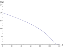
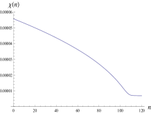
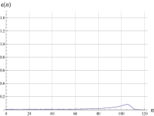
Figure 1: Plots of the dimensionless scalar $\phi(n)$ (on the left), the dimensionless Hubble parameter $\chi(n)$ (middle) and the first slow roll parameter $\epsilon(n)$ (on the right) for the quantum-corrected model (26) with Yukawa coupling $\lambda=5\times 10^{-4}$. Even with this minuscule value of $\lambda$ the geometry approaches de Sitter at a reduced scale.

We did not start to see evolution until values of about $\lambda\sim 10^{-3}$. Figure 1 shows the result for $\lambda=5\times 10^{-4}$. Although the model evolves noticeably for the first 100 e-foldings, there are considerable deviations from the classical result. These deviations become extreme at late times, for which the figure shows that the quantum-corrected model approaches de Sitter expansion at a reduced Hubble parameter.

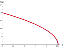
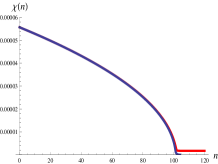
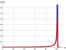
Figure 2: Results from the classical model $U=\frac{1}{2}k^{2}\phi^{2}$ (in blue) versus the quantum corrected model (26) (in red) assuming the inflaton is Yukawa-coupled to a fermion. We show the dimensionless scalar $\phi(n)$ (left hand graph), the dimensionless Hubble parameter $\chi(n)$ (middle graph), and the first slow roll parameter $\epsilon(n)$ (right hand graph). The value of the Yukawa coupling was chosen to be $\lambda=1.15\times 10^{-4}$.

Figure 2 compares the quantum-corrected model (in red) with the classical results (in blue) for the even smaller Yukawa coupling of $\lambda=1.15\times 10^{-4}$. Although the two models seem to track for about 100 e-foldings, inflation ends in the classical model whereas the quantum corrected model again approaches de Sitter. The numerical analysis shows that $\chi$ is visibly nonzero in this de Sitter phase whereas $\phi$ is very small.

To see that the late de Sitter phase is generic, note that when $\phi(n)\ll\phi(0)$ the ratio $\lambda\phi(n)/\chi(0)\ll 1$, so we can neglect the subtraction term in (26). Now write the modified Friedmann equation (18) and the scalar evolution equation (20) under the assumption that $\phi(n)$ and $\chi(n)$ are both constant,

$$3\chi^{2} = \frac{1}{2}k^{2}\phi^{2}+\frac{\chi^{4}}{8\pi^{2}}\Bigl{[}3f(z)-zf^{\prime}(z)\Bigr{]}\;,$$ (28)

$$0 = \frac{1}{2}k^{2}\phi^{2}+\frac{\chi^{4}}{8\pi^{2}}\Bigl{[}-\frac{1}{2}zf^{\prime}(z)\Bigr{]}\;,$$ (29)

where $z=\lambda\phi(n)/\chi(n)$. There is no simple way to solve there equations analytically, but it is easy to generate an efficient numerical solution. First, subtract (29) from (28) to infer a relation between $\chi^{2}(n)$ and $z$,

$$\chi^{2}=\frac{24\pi^{2}}{3f(z)\!-\!\frac{1}{2}zf^{\prime}(z)}\;.$$ (30)

Now substitute (30) in (29) to derive an equation which determines $z$ in terms of the parameters $k^{2}$ and $\lambda$,

$$\frac{k^{2}}{\lambda^{2}}=\frac{3z^{-1}f^{\prime}(z)}{3f(z)\!-\!\frac{1}{2}zf^{\prime}(z)}\;.$$ (31)

The right hand side of (31) is a complicated function of $z$ but one can check numerically that it is monotonically decreasing. Further, the known asymptotic forms for $f(z)$ [13],

$${\rm Large}\;z : f(z)\longrightarrow z^{4}\ln(z)+O(z^{4})\;,$$ (32)

$${\rm Small}\;z : f(z)\longrightarrow\alpha z^{6}-\beta z^{8}+O(z^{10})\;,$$ (33)

imply that the right hand side of (31) diverges like $18\alpha/\beta z^{4}$ for small $z$, and goes to zero like $12/z^{2}$ for large $z$. This means there is a unique solution for $z$ in terms of $k^{2}/\lambda^{2}$. Hence the desired procedure is:

1. Given the parameters $k$ and $\lambda$, use expression (31) to solve for $z$;

2. Substitute $z$ into (30) to compute $\chi^{2}$; and

3. Compute $\phi^{2}=z^{2}\chi^{2}/\lambda^{2}$.

Because the late de Sitter phase emerges from numerical analysis it is no doubt stable. Demonstrating this analytically amounts to studying how $\frac{\partial U}{\partial\phi}$ varies when $\phi$ is changed. Note first that altering $\phi$ induces corresponding changes in $\chi$ through relation (28),

$${\rm Eqn.\ (\ref{F1new})}\Longrightarrow\frac{\phi}{\chi}\frac{d\chi}{d\phi}=\frac{-3zf^{\prime}(z)\!+\!z^{2}f^{\prime\prime}(z)}{6f(z)\!-\!5zf^{\prime}(z)\!+\!z^{2}f^{\prime\prime}(z)}\;.$$ (34)

(Relation (34) has been simplified using relation (29).) A straightforward calculation then reveals that the total derivative of $\frac{\partial U}{\partial\phi}$ is,

$$\phi^{2}\frac{d}{d\phi}\Bigl{(}\frac{\partial U}{\partial\phi}\Bigr{)}=\frac{\chi^{4}}{8\pi^{2}}\frac{[6f(zf^{\prime}\!-\!z^{2}f^{\prime\prime})\!+\!4(zf^{\prime})^{2}]}{6f\!-\!5zf^{\prime}\!+\!z^{2}f^{\prime\prime}}\;.$$ (35)

One can see that this is positive in the small $z$ regime (33), but not in the regime of large $z$ (32). Because the graphs in Figures 1 and 2 suggest the small $z$ regime we conclude that the late de Sitter phase is stable.

It is not simple to derive a formula for the effective cosmological constant of the late de Sitter phase because it depends so strongly on the dimensionless function $f(z)$ through relation (30). If one assumes the small $z$ form (33) then the effective cosmological constant is,

$$\Lambda=3H^{2}=\frac{3\chi^{2}}{8\pi G}\longrightarrow\frac{2\pi^{2}\beta k^{2}}{9\alpha^{2}\lambda^{4}}\!\times\!m^{2}$$ (36)

Some of the numbers in relation (36) are fixed: $\alpha\simeq 0.11$, $\beta\simeq 0.014$ and $k^{2}\simeq 4.6\times 10^{-11}$. Using the value $\lambda=1.15\times 10^{-4}$ of Figure 2 gives $\Lambda\simeq(7\times 10^{5})\times m^{2}$. However, our formula (36) predicts that decreasing $\lambda$ should increase $\Lambda$, whereas exactly the opposite trend is apparent in the transition from Figure 1, with $\lambda=5\times 10^{-4}$, to Figure 2, with $\lambda=1.15\times 10^{-4}$. We attribute the apparent contradiction to the fact that ratio $k^{2}/\lambda^{2}$ is in neither case large enough (it is about $2\times 10^{-4}$ for Figure 1 and about $3\times 10^{-3}$ for Figure 2) to justify the small $z$ approximation (33) for $f(z)$.

Finally, we consider whether the small positive cosmological constant of the late de Sitter phase can be absorbed by adding a negative constant $-K$ to the potential $U(\phi,\chi)$, which changes (28) to,

$$3\chi^{2}=-K+\frac{1}{2}k^{2}\phi^{2}+\frac{\chi^{4}}{8\pi^{2}}\Bigl{[}3f(z)\!-\!zf^{\prime}(z)\Bigr{]}\;.$$ (37)

The scalar equation (29) is unchanged so relation (30) becomes,

$$\chi^{2}=\frac{24\pi^{2}}{3f\!-\!\frac{1}{2}zf^{\prime}}\Biggl{\{}\frac{1}{2}+\frac{1}{2}\sqrt{1+\frac{K}{18\pi^{2}}\Bigl{[}3f\!-\!\frac{1}{2}zf^{\prime}\Bigr{]}}\Biggr{\}}.$$ (38)

And the relation which fixes $z$ changes from (31) to,

$$\frac{k^{2}}{\lambda^{2}}=\frac{3z^{-1}f^{\prime}(z)}{3f(z)\!-\!\frac{1}{2}zf^{\prime}(z)}\Biggl{\{}\frac{1}{2}+\frac{1}{2}\sqrt{1+\frac{K}{18\pi^{2}}\Bigl{[}3f\!-\!\frac{1}{2}zf^{\prime}\Bigr{]}}\Biggr{\}}.$$ (39)

Although the function on the right hand side of (39) still diverges as $z\rightarrow 0$, it no longer vanishes for $z\rightarrow\infty$. Hence one can certainly solve for $z$ when $\lambda$ is very small, but making $\lambda$ larger eventually precludes a solution. When there is a solution, its value will generally be larger than for $K=0$, and this generally leads to a smaller value of $\chi$. However, note that any value of $K>0$ for which there is a solution to equation (39) will correspond to a nonzero value of $\chi$. So we conclude that it is only possible to avoid the late de Sitter phase by making $K$ large enough that (39) has no solution.

4.2 Charged Inflaton Coupled to Gauge Bosons

The quantum-corrected dimensionless potential for a charged inflaton (with charge $q$) is,

$$U(\phi,\chi)=k^{2}\phi^{*}\phi+\frac{3\chi^{4}}{8\pi^{2}}f\Bigl{(}\frac{q^{2}\phi^{*}\phi}{\chi^{2}}\Bigr{)}-\frac{3\chi^{4}(0)}{8\pi^{2}}f\Bigl{(}\frac{q^{2}\phi^{*}\phi}{\chi^{2}(0)}\Bigr{)}\;.$$ (40)

The function $f(z)$ appropriate for a gauge boson is [11, 12],

$$f(z)=-\Bigl{(}1\!-\!2\gamma\Bigr{)}z-\Bigl{(}\frac{3}{2}\!-\!\gamma\Bigr{)}z^{2}$$ (41)

$$\hskip 56.9055pt+\int_{0}^{z}\!\!\!dx\,(1\!+\!x)\Biggl{[}\psi\Bigl{(}\frac{3}{2}\!+\!\frac{1}{2}\sqrt{1\!-\!8x}\,\Bigr{)}+\psi\Bigl{(}\frac{3}{2}\!-\!\frac{1}{2}\sqrt{1\!-\!8x}\,\Bigr{)}\Biggr{]}\;.\qquad$$

Of course a bosonic quantum correction adds to the vacuum energy, which makes the result opposite to that for fermions. For order one values of the inflaton charge $q$ the two quantum corrections totally dominate the classical term and inflation ends almost instantly. Making inflation last for 60 e-foldings requires the minuscule value of $q^{2}=5.5\times 10^{-6}e^{2}$, the effects of which are shown in Figure 3. Even with this charge there are noticeable deviations from the classical model, in particular, a much more sudden end to inflation.

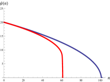
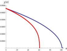
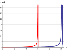
Figure 3: Results from the classical model $U=\frac{1}{2}k^{2}\phi^{2}$ (in blue) versus the quantum corrected model (40) (in red) assuming a charged inflaton (with charge $q^{2}=5.5\times 10^{-6}e^{2}$) is minimally coupled to vector bosons. The left hand graph shows the scalar $\phi(n)$, the middle graph gives the dimensionless Hubble parameter $\chi(n)$, and the right hand graph depicts the first slow roll parameter $\epsilon(n)$.

5 Discussion

Scalar-driven inflation suffers from many fine-tuning problems. These are exacerbated by the need to couple the inflaton to normal matter in order to make reheating efficient. Quantum fluctuations of normal matter induce cosmological Coleman-Weinberg potentials which are not Planck-suppressed and, for de Sitter, depend in complicated ways on the dimensionless ratio of the square of the coupling constant times the inflaton over the Hubble parameter. Although exact results do not exist for more general backgrounds, it is possible to show that the factors of “$H^{2}$” are not generally constant, nor even local functionals of the metric. The absence of locality restricts the extent to which these corrections can be subtracted off. The purpose of this paper was to study the consequences to inflation under two assumptions:

1. The de Sitter Hubble constant is replaced by the evolving Hubble parameter $H(t)$ in the cosmological Coleman-Weinberg potentials; and

2. The potentials are completely subtracted at the beginning of inflation with the de Sitter Hubble constant replaced by the initial value of the Hubble parameter.

In section 3 we derived the appropriate generalizations to the Friedmann equations, and we cast the formalism in terms of dimensionless variables evolved with respect to the number of e-foldings from inflation. In section 4 we numerically evolved the $m^{2}\varphi^{2}$ model, assuming first that the inflaton is Yukawa-coupled to a fermion and then that a charged inflaton is minimally coupled to a gauge boson. The results were catastrophic. For the case of fermions inflation never really ends, no matter how small the Yukawa coupling. For bosons the quantum-corrected effective potential causes inflation to end almost  instantly unless the charge is chosen so small as to make reheating problematic.

These results are completely unacceptable for scalar-driven inflation. However, it is not known how much they depend upon the particular subtraction scheme we studied. It is worth investigating subtractions based on replacing the factors of “$H^{2}$” by $\frac{1}{12}R$. That replacement would be perfect for the de Sitter approximation to the Coleman-Weinberg potential, but there is still a difference between any local subtraction and the nonlocal Coleman-Weinberg potential it attempts to cancel. To study this difference we would need a more refined analysis of the nonlocal Coleman-Weinberg potential. In particular, what is a generally applicable approximation for the de Sitter factors of “$H^{2}$”? Attempting to answer this question seems worthwhile in view of the crippling potential problem to the viability of scalar-driven inflation that the current study has exposed.

Another potential solution is to couple derivatives of the inflaton to ordinary matter, for example $-\frac{1}{M^{3}}\partial_{\mu}\varphi\partial_{\nu}\varphi g^{\mu\nu}\overline{\psi}\psi\sqrt{-g}$, where $M$ is some mass scale. For small enough $M$ such a coupling would still be effective at communicating inflaton kinetic energy to the matter sector, and it has the virtue of preserving the (approximate) shift symmetry which is strongly suggested by the data. Of course the quantum corrections from such a coupling make no change at all in the inflaton effective potential, however, they do change the inflaton kinetic energy in ways that may be problematic. On de Sitter background the induced effective kinetic energy is closely related to the induced effective potential for nonderivative couplings,

$${\rm Nonderivative} \Longrightarrow -\frac{H^{4}}{8\pi^{2}}f\Bigl{(}\frac{\lambda\varphi}{H}\Bigr{)}\;,$$ (42)

$${\rm Derivative} \Longrightarrow -\frac{H^{4}}{8\pi^{2}}f\Bigl{(}\frac{\partial_{\mu}\varphi\partial_{\nu}\varphi g^{\mu\nu}}{M^{3}H}\Bigr{)}\;.$$ (43)

What emerges from (43) is a quantum-induced k-essence model. Instead of order one changes in the inflaton potential we must now confront order one changes in the kinetic energy, which can of course alter the inflationary geometry, the scalar and tensor power spectra and the reheat temperature. K-essence models sometimes also permit super-luminal propagation. It would be fascinating to make a quantitative study of the various consequences.

Acknowledgements

This work was partially supported by Taiwan MOST grants 103-2112-M-006-001-MY3 and 106-2112-M-006-008-; by NSF grants PHY-1506513 and PHY-1806218; and by the Institute for Fundamental Theory at the University of Florida.

References

- [1] P. A. R. Ade et al. [Planck Collaboration], Astron. Astrophys. 594, A20 (2016) doi:10.1051/0004-6361/201525898 [arXiv:1502.02114 [astro-ph.CO]].
- [2] A. Ijjas, P. J. Steinhardt and A. Loeb, Phys. Lett. B 723, 261 (2013) doi:10.1016/j.physletb.2013.05.023 [arXiv:1304.2785 [astro-ph.CO]].
- [3] A. H. Guth, D. I. Kaiser and Y. Nomura, Phys. Lett. B 733, 112 (2014) doi:10.1016/j.physletb.2014.03.020 [arXiv:1312.7619 [astro-ph.CO]].
- [4] A. Linde, doi:10.1093/acprof:oso/9780198728856.003.0006 arXiv:1402.0526 [hep-th].
- [5] A. Ijjas, P. J. Steinhardt and A. Loeb, Phys. Lett. B 736, 142 (2014) doi:10.1016/j.physletb.2014.07.012 [arXiv:1402.6980 [astro-ph.CO]].
- [6] S. R. Coleman and E. J. Weinberg, Phys. Rev. D 7, 1888 (1973). doi:10.1103/PhysRevD.7.1888
- [7] D. R. Green, Phys. Rev. D 76, 103504 (2007) doi:10.1103/PhysRevD.76.103504 [arXiv:0707.3832 [hep-th]].
- [8] T. M. Janssen, S. P. Miao, T. Prokopec and R. P. Woodard, Class. Quant. Grav. 25, 245013 (2008) doi:10.1088/0264-9381/25/24/245013 [arXiv:0808.2449 [gr-qc]].
- [9] P. Candelas and D. J. Raine, Phys. Rev. D 12, 965 (1975). doi:10.1103/PhysRevD.12.965
- [10] S. P. Miao and R. P. Woodard, Phys. Rev. D 74, 044019 (2006) doi:10.1103/PhysRevD.74.044019 [gr-qc/0602110].
- [11] B. Allen, Nucl. Phys. B 226, 228 (1983). doi:10.1016/0550-3213(83)90470-4
- [12] T. Prokopec, N. C. Tsamis and R. P. Woodard, Annals Phys. 323, 1324 (2008) doi:10.1016/j.aop.2007.08.008 [arXiv:0707.0847 [gr-qc]].
- [13] S. P. Miao and R. P. Woodard, JCAP 1509, no. 09, 022 (2015) doi:10.1088/1475-7516/2015/09/022, 10.1088/1475-7516/2015/9/022 [arXiv:1506.07306 [astro-ph.CO]].
- [14] J. Mielczarek, Phys. Rev. D 83, 023502 (2011) doi:10.1103/PhysRevD.83.023502 [arXiv:1009.2359 [astro-ph.CO]].
- [15] J. Martin and C. Ringeval, Phys. Rev. D 82, 023511 (2010) doi:10.1103/PhysRevD.82.023511 [arXiv:1004.5525 [astro-ph.CO]].
- [16] L. Kofman, A. D. Linde and A. A. Starobinsky, Phys. Rev. D 56, 3258 (1997) doi:10.1103/PhysRevD.56.3258 [hep-ph/9704452].
- [17] P. B. Greene, L. Kofman, A. D. Linde and A. A. Starobinsky, Phys. Rev. D 56, 6175 (1997) doi:10.1103/PhysRevD.56.6175 [hep-ph/9705347].
- [18] R. S. Palais, Commun. Math. Phys. 69, no. 1, 19 (1979). doi:10.1007/BF01941322
- [19] C. G. Torre, AIP Conf. Proc. 1360, 63 (2011) doi:10.1063/1.3599128 [arXiv:1011.3429 [math-ph]].