Semi-Dynamic Load Balancing: Efficient Distributed Learning in Non-Dedicated Environments

Abstract.

Machine learning (ML) models are increasingly trained in clusters with non-dedicated workers possessing heterogeneous resources. In such scenarios, model training efficiency can be negatively affected by stragglers—workers that run much slower than others. Efficient model training requires eliminating such stragglers, yet for modern ML workloads, existing load balancing strategies are inefficient and even infeasible. In this paper, we propose a novel strategy called semi-dynamic load balancing to eliminate stragglers of distributed ML workloads. The key insight is that ML workers shall be load-balanced at iteration boundaries, being non-intrusive to intra-iteration execution. We develop LB-BSP based on such an insight, which is an integrated worker coordination mechanism that adapts workers’ load to their instantaneous processing capabilities by right-sizing the sample batches at the synchronization barriers. We have custom-designed the batch sizing algorithm respectively for CPU and GPU clusters based on their own characteristics. LB-BSP has been implemented as a Python module for ML frameworks like TensorFlow and PyTorch. Our EC2 deployment confirms that LB-BSP is practical, effective and light-weight, and is able to accelerating distributed training by up to $54\%$.

1. Introduction

Machine learning (ML) models, such as deep neural networks, are widely used for a range of applications to attain state-of-the-art performance (Krizhevsky et al., 2012; Farabet et al., 2013; Collobert et al., 2011; Sutskever et al., 2014). Owing to their compute-intensive nature, ML models are often trained in a distributed manner (Dean et al., 2012; Li et al., 2014a; Chilimbi et al., 2014; Abadi et al., 2016): many worker threads iteratively process small subsets of the training data (i.e., sample batches), and use the computed updates to refine the global model parameters.

With the surge of ML training demands, it has become increasingly common to serve ML jobs in non-dedicated environments, e.g., with heterogeneous hardware from spot markets (gpu, 2019), or with time-varying resources from shared production clusters (Jeon et al., 2018; Xiao et al., 2018; Hazelwood et al., 2018). In such cases, workers with less capable resources would progress slower and become stragglers. Under the popular Bulk Synchronous Parallel (BSP) scheme, fast workers have to wait for slow ones at the end of each iteration, and stragglers would thus impair the model training efficiency.

To mitigate the negative effect of stragglers, a large number of mechanisms have been developed in the literature. For example, some (Dean et al., 2012; Ho et al., 2013; Cui et al., 2014) have proposed to relax the synchronization barriers to avoid end-of-iteration resource wastage, yet this negatively affects the update quality and requires more iterations for models to converge. In fact, stragglers in non-dedicated clusters are mainly caused by the mismatch between workers’ load and their processing capability. In response, the most effective strategy to eliminate stragglers is to balance the load of workers according to their instantaneous processing capability.

Nonetheless, ML workloads pose new challenges to the load balancing community. Existing load balancing schemes designed for traditional multi-core or big data scenarios can be broadly classified into two categories: static and dynamic load balancing (section 2.2.3). Yet, different from those traditional workloads such as HPC processing (Blumofe and Leiserson, 1999; Dinan et al., 2009) or MapReduce (Dean and Ghemawat, 2010), ML computations are highly structured (with thousands of short iterations) and also tensor-based (samples in each iteration are packaged into a non-divisible matrix for fast processing). Static load balancing approaches (Kokilavani et al., 2011; Samal and Mishra, 2013; Tang and Chanson, 2000) are not aware of runtime resource variations, and dynamic approaches (Yang and He, 2018; Acun and Kale, 2016; Harlap et al., 2016), which are mainly based on work stealing (Blumofe and Leiserson, 1999; Dinan et al., 2009; Acar et al., 2013), are also deficient for ML workloads. First, work stealing usually requires fine-grained worker progress monitoring and runtime load migration, which is inefficient for an iterative model training process. Second, runtime load migration assumes that samples are processed one by one, which is indeed incompatible with the style of tensor-based processing in modern ML frameworks (Abadi et al., 2016; Chen et al., 2015; PyT, 2020).

In this paper, we design a new load balancing strategy for distributed model training workloads, called semi-dynamic load balancing. In broad strokes, the high-level idea is to perform all load balancing actions—worker monitoring, straggler identification and load redistribution—on the iteration boundaries, with load adjustment enforced by tuning each worker’s sample batch size. Following such a high-level idea, we propose Load-Balanced Bulk Synchronous Parallel (LB-BSP), a composite scheme atop BSP that seeks to equalize all the workers’ batch processing times by speculatively configuring their batch sizes at the synchronization barriers. An immediate question is then how to set the batch size at the synchronization barriers for the best load balancing effect in the upcoming iteration. This evolves into different challenges for CPU and GPU clusters that are two typical platform types for distributed learning.

For a CPU worker, our profiling work (section 3.2.1) shows that its batch processing time is proportional to its batch size, with the proportion coefficient representing the instantaneous sample processing capability. In shared clusters, such a coefficient may vary drastically with the temporal resources (Hazelwood et al., 2018; Reiss et al., 2012), and thus shall be predicted prior to each iteration. For this purpose, we employ a special kind of recurrent neural network called NARX (Diaconescu, 2008), which can make accurate performance predictions by taking into account the driving resources such as CPU and memory.

In multi-tenant GPU clusters (Jeon et al., 2018; Peng et al., 2018; Xiao et al., 2018; Gu et al., 2019), a GPU is usually dedicated to one worker without sharing. But the relationship between a GPU worker’s batch processing time and batch size is not proportional and difficult to profile at runtime (section 3.3.1). Therefore, instead of the profiling-based analytical methods, we propose an iterative batch size tuning algorithm that can efficiently approximate the load-balanced state without prior knowledge.

Furthermore, while our method of worker-adaptive batch sizing can effectively eliminate stragglers, it inevitably results in non-uniform batch sizes among different workers, which may negatively affect the training accuracy. To ensure that model training process can still converge correctly even with inconsistent batch sizes, we further propose weighted gradient aggregation, in which the batch size of each worker is used as the weight of its gradient in aggregation.

We have implemented LB-BSP with a Python module that can be easily integrated into existing ML frameworks like TensorFlow (Abadi et al., 2016), PyTorch (PyT, 2020) and MXNet (Chen et al., 2015). Our experiments on Amazon EC2 with popular benchmark training workloads show that LB-BSP can effectively eliminate stragglers in non-dedicated clusters, achieving near-optimal training efficiency with negligible overhead. In particular, in a 16-node heterogeneous GPU cluster, LB-BSP outperforms existing worker coordination schemes by over $54\%$; and in a 32-node shared CPU cluster, it attains an improvement of up to 38.7% over state-of-the-art straggler mitigating approaches.

2. Background and Motivation

2.1. Research Background

Basics of Machine Learning. Given a machine learning (ML) model, the objective of model training process is to find the model parameters $\omega^{\star}$ that can minimize the loss function $L(\omega)$ over the labeled training dataset $S$, i.e.,

(1) $$\omega^{\star}=\arg\min_{\omega}{L(\omega)}=\arg\min_{\omega}\frac{1}{|S|}\sum\nolimits_{s\in S}{l(s,\omega)}.$$

Here, $l(s,\omega)$ is the loss value for a data sample $s$ in $S$.

A popular training algorithm is mini-batch Stochastic Gradient Descent (Dean et al., 2012; Li et al., 2014b), or simply SGD. Its basic idea is to iteratively refine model parameters $\omega$ with the gradients $g$ calculated from the sample batches, i.e.,

(2) $$\omega^{k+1}=\omega^{k}-\eta g^{k}\textnormal{, where }g^{k}=\frac{1}{|B^{k}|}\sum\nolimits_{s\in B^{k}}{\nabla l(s,\omega^{k})}.$$

Here, $k$ is the iteration number, $B^{k}$ is a batch randomly sampled from the training dataset $S$, and $\eta$ is the learning rate. Such training iterations would repeat until the model parameters $\omega$ finally converge.

Given the stochastic nature of SGD, the relationship between training completion (i.e., model convergence) and the sample processing amount is not deterministic, and the model training efficiency is usually decoupled into two parts: hardware efficiency—how fast each iteration can be finished, and statistical efficiency—how many iterations it takes towards model convergence. Therefore, efficient model training requires both high hardware efficiency and high statistical efficiency.

Distributed Model Training. To accelerate the model training process, it has been increasingly common to train ML models in a distributed manner, with a pool of parallel workers. Those workers typically collaborate in a synchronous mode (i.e., BSP) (Zhang et al., 2017b; Goyal et al., 2017; Cui et al., 2016), under the Parameter Server (PS) (Ho et al., 2013; Li et al., 2014a; Cui et al., 2016) or All-Reduce (Goyal et al., 2017) architecture.

With the widespread adoption of ML techniques, distributed model training is now conducted in various cluster environments, and we broadly classify them into two types: dedicated and non-dedicated clusters.

(1) Dedicated clusters implies that the clusters are homogeneous, and are composed of cutting-edge GPUs dedicated to one training job. For example, Facebook’s well-known work of training ImageNet in one hour (Goyal et al., 2017) is conducted in such a dedicated cluster with 256 Tesla P100 GPUs. While dedicated clusters can yield high training efficiency, they are expensive to maintain and not widely accessible (Goyal et al., 2017; Jia et al., 2018).

(2) Non-dedicated clusters refer to the clusters that are composed of heterogeneous hardware or shared by multiple tenants. Since newer CPU or GPU generations get released at a rapid pace, a budget-limited user may choose to train models with a set of heterogeneous hardware (e.g., GPUs) from the local inventory (Li et al., 2018; Park et al., 2020) or from spot markets such as Amazon EC2 (ec2, 2020; gpu, 2019; Jiang et al., 2017) or FloydHub (flo, 2020). Meanwhile, large companies (Hazelwood et al., 2018; Jeon et al., 2018) may host multiple ML jobs in their production clusters with mixed hardware types; for fairness, users may be allocated heterogeneous hardware (Chaudhary et al., 2020; Mahajan et al., 2020; Narayanan et al., 2020), and their resource allocation may also be dynamically adjusted by cluster schedulers for resource packing purpose (Xiao et al., 2018; Gu et al., 2019).

While model training in non-dedicated clusters is increasingly common, it is far less efficient than training in dedicated clusters due to the straggler problem, which is more severe in non-dedicated clusters. For clarity, we classify stragglers into two groups: non-deterministic and deterministic stragglers.

(1) Non-deterministic stragglers are caused by temporary disturbance like OS jitter or garbage collection, usually being transient and slight. They occur and vanish naturally in both dedicated and non-dedicated clusters.

(2) Deterministic stragglers are caused by the heterogeneity of worker resource quality or quantity, and are often severe and long-lasting. They occur only in non-dedicated clusters.

Compared with non-deterministic stragglers, deterministic stragglers are more harmful to distributed model training, by forcing fast workers to always wait for the slowest one in each iteration if under the popular BSP scheme. With the increasing prevalence of non-dedicated clusters, it is thus in urgent need to tame such deterministic stragglers.

2.2. Related Work

Stragglers have long been a thorny problem in distributed computing systems, and in the research literature there have been many attempts to tackle such a problem.

2.2.1. Bypassing Stragglers with Relaxed Synchronization

To exempt fast workers from waiting for stragglers, two worker coordinating schemes with the synchronization constraint compromised have been proposed: ASynchronous Parallel (ASP), and Stale Synchronous Parallel (SSP).

ASP. In ASP (Dean et al., 2012), workers can independently proceed to the next iteration without waiting for others. In this way, ASP wastes no compute cycles and attains high hardware efficiency. However, the price paid is low statistical efficiency: without global synchronization, the gradient computation often uses stale parameters, which yields low-quality updates and requires more iterations to converge (Ho et al., 2013; Langford et al., 2009).

SSP. SSP (Ho et al., 2013; Cui et al., 2014) comes as a middle ground between BSP and ASP. In SSP, fast workers wait for the stragglers only when the parameter staleness reaches a particular threshold. SSP can then accelerate ML iterations while providing a convergence guarantee. Nonetheless, SSP focuses primarily on non-deterministic stragglers, expecting the straggling workers to catch up soon in later iterations. This works for homogeneous clusters, but in non-dedicated clusters the deterministic stragglers may persist across many consecutive iterations, and the staleness quota of SSP can be quickly used up. After the quota is used up, fast workers will have to wait for the slowest ones in almost every iteration, leading to low hardware efficiency.

2.2.2. Mitigating Stragglers by Redundant Execution

Redundant execution (Ananthanarayanan et al., 2013; Zaharia et al., 2008) is widely adopted to mitigate stragglers in traditional data analytics frameworks like MapReduce (Dean and Ghemawat, 2010) and Spark (Zaharia et al., 2012). It launches multiple copies of a straggling task and accepts results only from the one that finishes first. It has also been recently introduced to the context of distributed machine learning: Chen et al. (Chen et al., 2016) proposed to train deep neural models with extra backup workers and to use gradients from those workers finishing the earliest. However, redundant execution is merely a suboptimal solution: it mitigates some worst-case stragglers but fails to eliminate all of the stragglers completely. Even worse, backup workers themselves would consume additional resources.

2.2.3. Eliminating Stragglers by Load Balancing

The solutions we have discussed so far are agnostic to the root causes of stragglers, and they do not seek to prevent stragglers from occurring. As we mentioned, efficiency loss in non-dedicated clusters is primarily caused by deterministic stragglers, whose root cause is very clear—the mismatch between the workers’ loads and their processing capabilities (existing ML frameworks (Abadi et al., 2016; Chen et al., 2015; Jia et al., 2014) blindly assign a uniform batch load to all the workers). Therefore, to fundamentally eliminate such deterministic stragglers related to load-resource mismatching, we should resort to load balancing techniques. Load balancing is a classical research topic (Al Nuaimi et al., 2012) in the parallel processing community, and existing solutions can be broadly classified into two types: static and dynamic load balancing.

Static Load Balancing. Static load balancing strategies (Kokilavani et al., 2011; Samal and Mishra, 2013; Tang and Chanson, 2000; Tantawi and Towsley, 1985) set a constant load for each worker—as the execution commences—under a given scheme like Round-Robin (Samal and Mishra, 2013) or with some static knowledge of the worker status (Tang and Chanson, 2000; Tantawi and Towsley, 1985). It does not require real-time progress measurements or cross-worker communication, but cannot react to resource variations that are common in non-dedicated clusters.

Dynamic Load Balancing. Dynamic load balancing strategies use work-stealing or work-shedding to redistribute load from heavily-loaded workers to lightly-loaded ones at runtime (Blumofe and Leiserson, 1999; Dinan et al., 2009; Acar et al., 2013; Yang and He, 2018; Acun and Kale, 2016). They are mostly developed for traditional task-based parallel programming models in multi-core or HPC systems. Recently, FlexRR (Harlap et al., 2016) adopted such a dynamic strategy to tackle (non-deterministic) stragglers for ML workloads. It measures the workers’ instantaneous progress at a fine granularity (100 checks per iteration); once a straggling worker lags behind others over a given threshold, it would yield certain sample processing load to a faster worker. Responding to dynamic changes of resources, dynamic load balancing schemes usually outperform static ones, but the cost paid is much higher computation and communication overhead (for progress monitoring, status collection and workload migration), which is not desirable in resource-intensive ML training. To reduce such overhead, FlexRR conducts straggler detection and load migration within designated worker groups, which nonetheless leads to suboptimal load balancing performance due to its lack of global coordination.

Moreover, a key assumption of dynamic load balancing strategies is that, workloads shall be processed in a sequential manner so that they can be arbitrarily split and transferred at runtime. However, this is not true for modern ML workloads. Training ML models is compute-intensive, and parallel-processing accelerators like GPUs are commonly used in practice, for which sequential processing is highly inefficient (section 3.3.1). To fully exploit the power of such accelerators, mainstream ML frameworks wrap all the samples in a batch as a tensor matrix (e.g., a Tensor in TensorFlow/PyTorch, or an NDArray in MXNet), which is concurrently processed in a single round. Given such all-or-nothing processing, it is hard to measure fine-grained worker progress or adjust its load in the midst of an iteration, making dynamic load balancing simply infeasible.

2.3. Semi-Dynamic Load Balancing

Objectives. Based on our discussions so far, our objective is to develop a load balancing strategy for ML workloads with the following properties:

(1) Practicality. It should be compatible with the style of tensor-based processing in existing ML frameworks.

(2) Effectiveness. It should be aware of the instantaneous worker execution status, and adjust the workers’ load in a coordinated manner to attain the best load balancing effect.

(3) Efficiency. It should not interfere with regular processing within each iteration, and should try to be light-weight by avoiding cross-worker data movement.

Design Philosophy. To meet these objectives, we propose a new load balancing strategy called semi-dynamic load balancing. Tailored for ML workloads, its basic idea is to have workers’ load be static within each iteration but dynamic across different iterations. In particular, we offload all load balancing operations—status measurements, straggler detection and load adjustment—at the iteration boundaries of BSP, using the batch size as a tool for load tuning. This strategy is feasible and can satisfy all of our design objectives, which we rationalize from the following three aspects:

(1) Measuring worker status at iteration boundaries. Training iterations in modern ML frameworks are relatively short (in seconds or even sub-seconds, as we show later in Fig. 1 and Fig. 4), and these iterations share a high similarity because an identical computation graph is used in each iteration. Therefore, the execution status in recent iterations is a valuable reference for that of the near future, relieving the need for costly intra-iteration progress measurements.

(2) Detecting stragglers at BSP iteration boundaries. Under BSP there is a synchronization barrier at the end of each iteration, offering a natural opportunity to centralize all the workers’ status information and optimize, with a global view, their load for the best load balancing effect.

(3) Adjusting load by tuning the batch size at iteration boundaries. The batch size is a hyper-parameter that, as each iteration commences, dictates how many samples should be encapsulated into a tensor batch for processing in that iteration. It accurately controls a worker’s load because each sample consumes identical compute cycles. Besides, given the stochastic (i.e., sample-insensitive) nature of SGD, load migration can be realized by increasing the batch size of one worker and reducing that on another. This can avoid the communication overhead without compromising the training convergence.

In the next section, we show how the philosophy of semi-dynamic load balancing can be implemented in practice.

3. LB-BSP

In this section, we present Load-Balanced Bulk Synchronous Parallel (LB-BSP), an integrated scheme atop BSP, for efficient distributed learning in non-dedicated clusters. We start with the problem formulation of LB-BSP, and then elaborate our solutions for CPU and GPU clusters, respectively.

3.1. Problem Formulation

In each model training iteration, given the sample batch, a worker first calculates a local gradient and then remotely refines the global model. Here we refer to the entire duration as the batch processing time, denoted by $t$. It can be divided into two parts: computation time ($t^{p}$), which measures the time taken to compute the gradient, and communication time ($t^{m}$), which measures the time taken for data transmission.

In a nutshell, LB-BSP seeks to equalize $t$ on different workers by rightsizing their sample batches at the synchronization barriers. This can be formulated as an optimization problem. Given $n$ workers with the initial batch size ẋ, we want to find the worker batch sizes $\vec{x}=(x_{1},x_{2},...,x_{n})$ that can minimize the longest batch processing time among all workers, i.e.,

(3) $$\underset{\vec{x}=(x_{1},x_{2},...,x_{n})}{\text{min}} \underset{i\in\{1,2,...n\}}{\text{max}}t_{i},$$

  s.t. $$t_{i}=t^{p}_{i}+t^{m}_{i},\;i=1,\ldots,n;$$

$$t^{p}_{i}=\varGamma_{i}(x_{i}),\;i=1,\ldots,n;$$

$$\sum\nolimits_{i=1}^{n}{x_{i}}=X=n\text{\.{x}}.$$

Here $\varGamma_{i}(\cdot)$ is the function between worker-$i$’s computation time $t^{p}_{i}$ and its batch size $x_{i}$. The last constraint ensures that the total number of samples processed in each iteration remains the same as that in BSP. Table 1 summarizes the important notations used in the paper.

$\!t$	batch processing time	$x_{i}$	batch size on worker-$i$
$\!t^{p}$	computation time	ẋ	initial batch size
$\!t^{m}$	communication time	$X$	$n$ẋ ($n$ is worker number)
$\!\varGamma(\cdot)$	function between $t^{p}$ and $x$	$v$	sample processing speed

Table 1. Summary of important notations.

Solution Overview. Solving problem (3) poses different challenges to CPU and GPU clusters. In shared CPU clusters, $t_{i}$ increases linearly with $x_{i}$, but that ratio varies with the temporal resources. In GPU clusters, the relationship between $t_{i}$ and $x_{i}$ is non-linear and hard to profile at runtime. Based on their respective characteristics, we design an analytical method that directly configures the optimal $\vec{x}$ for CPU clusters (section 3.2), and a numerical method that iteratively approaches the optimal $\vec{x}$ for GPU clusters (section 3.3).

3.2. LB-BSP in CPU Clusters

We summarize some typical scenarios where models are trained in CPU clusters without accelerators like GPUs:

(1) Non-neural-network Model Training. Many traditional ML applications like Support Vector Machines (SVM) or Logistic Regression (LR) demand less computing resources than neural networks. They are usually trained in CPU clusters (Jiang et al., 2017; Hazelwood et al., 2018; Harlap et al., 2016; Zhang et al., 2017a).

(2) Non-urgent Model Training. Non-urgent ML tasks may also be trained in CPU clusters opportunistically with leftover resources (Le et al., 2020; Hazelwood et al., 2018). For example, to improve cluster utilization, Facebook trains some peripheral face recognition models with the off-peak portions of CPU servers in the diurnal cycle, where the CPU resources would otherwise be wasted (Hazelwood et al., 2018).

We next present the techniques to fully exploit available resources in such non-dedicated CPU clusters to attain the best model training efficiency.

3.2.1. Performance Characterization of CPU Workers

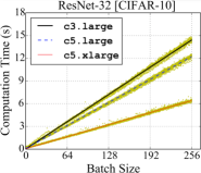
(a)

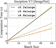
(b)

Figure 1. The relationship between computation time and batch size for different EC2 CPU instances.

Static Characteristics. To solve problem (3) for CPU clusters, we first characterize the static properties of CPU workers by measuring their performance against different batch size configurations when there is no resource contention.

(1) Negligible Communication Time: $t^{p}\gg t^{m}$ ($t\approx t^{p}$). Model training is a compute-intensive task for CPU workers, and with built-in optimizations (Zhang et al., 2017b) of modern ML frameworks, communication can be hidden by the long computation time ($t^{p}$). In our measurements on EC2, when training the Inception-V3 model on ImageNet dataset (introduced later in section 5.1) with 32 workers and one separate PS (c5.2xlarge instances with $\leq 10Gbps$ bandwidth), $t^{p}$ takes more than $99\%$ of the batch processing time $t$.

(2) Linear Relationship: $\varGamma(x)=x/v.$ As batch size quantifies the iteration load, for CPU processors the computation time $t^{p}$ is proportional to the batch size $x$. To confirm that, we respectively train the ResNet-32 and Inception-V3 model with different types of EC2 instances. We vary $x$ and record the corresponded computation time $t^{p}$ in Fig. 1, which in each case exhibits strong linearity between $x$ and $t^{p}$. Let $v$ be the ratio of $x$ to $t^{p}$, i.e., the sample processing speed, we then have $t\approx t^{p}=\varGamma(x)=x/v$.

Given the characteristics above, we solve optimization problem (3) with $x_{i}=\frac{v_{i}}{\sum\nolimits_{j=1}^{n}{v_{j}}}X$. Note that such an analytical method essentially merges straggler detection and elimination together. In a nutshell, to set the worker batch size for an upcoming iteration, we only need to know their sample processing speed in that iteration.

Challenges for LB-BSP in shared CPU clusters. Although a CPU worker’s batch size can be determined with its sample processing speed, when training with resource contention in shared clusters, that sample processing speed may vary dynamically. Therefore, to load-balance workers with adjustments only at the iteration boundaries, we need to predict their sample processing speed before the start of an iteration. As stragglers in non-dedicated CPU clusters can be deterministic and non-deterministic, an ideal prediction approach should be robust to non-deterministic perturbations to avoid over-reaction or oscillation. It should also react to deterministic resource variations quickly.

3.2.2. Predicting Sample Processing Speed

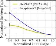
(a)

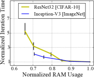
(b)

Figure 2. Sample processing speed is affected by CPU or memory resources. Measurements are conducted with the stress-ng tool (str, 2019) on a c5.2xlarge instance (with swap spaces enabled). The resource usage and iteration time are normalized by the monopolizing case. Each point is an average of $100$ iterations.

Potential Approaches. A simple solution is to use the last iteration’s speed or the Exponential Moving Average (EMA) speed as the predicted one. However, the former is not robust to temporary perturbations, and the latter cannot react quickly to drastic resource variations.

Speed prediction belongs to a classical research problem—time series prediction, for which many statistical or learning-based techniques have been proposed. As a statistical approach, Autoregressive Integrated Moving Average (ARIMA) (Ediger and Akar, 2007) makes predictions with statistics like average and deviation. Meanwhile, models based on Recurrent Neural Network (RNN) (Connor et al., 1994) (like plain RNN and LSTM (Hochreiter and Schmidhuber, 1997)), with the ability to maintain inner memory, have been applied in forecasting real-world time series like stock price (Rather et al., 2015) or transport flow (Polson and Sokolov, 2017).

However, the prediction performance of all the above approaches is limited by their blindness to the underlying resources. In fact, variations of the driving resources like CPU and memory closely relate to the instantaneous worker processing capability.

This is supported by Fig. 2, in which the model training processes are slowed down after we restrict their resource usage. Such driving resources can help to distinguish the deterministic straggling factors from random perturbations and make more accurate prediction. To this end, we find that Nonlinear AutoRegressive eXogenous (NARX) model (Gao and Er, 2003; Diaconescu, 2008) is a good fit for the prediction of sample processing speed.

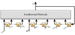
(a)

Figure 3. NARX architecture.

NARX Approach. The NARX model we use is basically an extended recurrent neural network that takes three series as inputs: past values of sample processing speed ($\boldsymbol{v}$), current and past values of the two driving resources—CPU and memory usage ($\boldsymbol{c}/\boldsymbol{m}$). Essentially, NARX aims to learn a nonlinear function $F(\cdot)$ between the predicted speed and a limited view (specified with a look-back window size) of the input series:

(4) $$\!\!v^{k}=F(v^{k-1},...,v^{k-d_{v}},c^{k},...,c^{k-d_{c}},m^{k},...,m^{k-d_{m}}).\!\!$$

Here $v^{k}$, $c^{k}$ and $m^{k}$ represent the value of speed, CPU and memory usage in iteration $k$, respectively; $d_{v}$, $d_{c}$ and $d_{m}$ represent the corresponded look-back window size of each series. Fig. 3 shows the unfolded architecture of the NARX model, in which the input series are fed into a feedforward neural network.

The batch size adjusting process with NARX is elaborated in Alg.1. In practice, to ensure high prediction accuracy, we maintain a NARX model for each worker, which is trained with the historical execution information (i.e., $\boldsymbol{v}$, $\boldsymbol{c}$ and $\boldsymbol{m}$). To avoid high model complexity, as in existing prediction works (Argyropoulos et al., 2016; Cadenas et al., 2016), the look-back window sizes for all the three input series are set to $2$, and we include only one hidden layer in the feedforward network. Such a simple model can avoid over-fitting and converge fast. Our later evaluation (section 5.4) confirms that such a NARX-based approach can make better predictions than other approaches we surveyed.

Algorithm 1 Batch Size Updating in CPU clusters

1:Input: {$x_{i}^{k-1}\!$}, {$t_{i}^{k-1}\!$}, {$c_{i}^{k}\!$}, {$m_{i}^{k}\!$} $\triangleright$ last batch size, last batch processing time, current cpu & memory usage of all the workers $\!(i\!\!=\!\!1,\!2,\!\!...,\!n)\!$

2:Require: past values of $\{v_{i}\},\{c_{i}\},\{m_{i}\},i=1,2,...,n$;

3:        $F_{i}(\cdot)$, $i=1,2,...,n.$ $\triangleright$ NARX model for each worker

4:procedure CPU_UpdateBatchSize($k$)

5:    $\!\!\!v_{i}^{k-1}\leftarrow x_{i}^{k-1}/t_{i}^{k-1},i$=$1,2,...,n.$

6:    $\!\!\!v_{i}^{k}\!\!=\!F_{i}(v_{i}^{k-1}\!\!,...,v_{i}^{k-d_{v}}\!,c_{i}^{k}\!,...,\!c_{i}^{k-d_{c}}\!\!,m_{i}^{k}\!,...,m_{i}^{k-d_{m}})$, $i$=$1,...,n.$

7:    $\!\!X\leftarrow\sum\nolimits_{i=1}^{n}{x_{i}^{k-1}}$

8:    $\!\!x_{i}^{k}=\frac{v_{i}^{k}}{\sum\nolimits_{j=1}^{n}{v_{j}^{k}}}\cdot X$, $i=1,2,...,n.$

9:    round $x_{i}^{k}(i=1,...,n)$ to integers with $\sum\nolimits_{i=1}^{n}{x_{i}^{k}}=X$.

10:    return {$x_{i}^{k}$}

3.3. LB-BSP in GPU Clusters

With strong parallel processing capability, GPUs are the workhorse hardware for training deep neural networks (Zhang et al., 2017b; Goyal et al., 2017; Jeon et al., 2018). As elaborated in section 2.1, neural network models may be trained in non-dedicated GPU clusters: with heterogeneous GPU instances from the spot markets (flo, 2020; gpu, 2019), or in shared GPU clusters (Jeon et al., 2018; Peng et al., 2018; Xiao et al., 2018; Gu et al., 2019) where workers may inter-connect at different locality levels and be migrated across machines for resource consolidation. Nonetheless, implementing LB-BSP in non-dedicated GPU clusters renders a challenge different with that in CPU clusters. In this part, we first characterize the performance of standalone GPU workers, and then present our LB-BSP algorithm for GPU clusters.

3.3.1. Performance Characterization of GPU Workers

Static Characteristics. To solve problem (3) for GPU clusters, we first profile the static properties of GPU workers.

(1) Non-negligible Communication Time: $t^{p}\not\gg t^{m}$ ($t\not\approx t^{p}$). Computations on GPU workers are usually orders of magnitude faster than CPU workers. Therefore, the communication time in each iteration is no longer negligible when compared with the computation time (Zhang et al., 2017b).

(2) Non-negligible GPU Launching Overhead: $\varGamma(0)>0$. Fig. 4 shows the relationship $\varGamma(\cdot)$ between $t^{p}$ and $x$ for different GPU types. Even for a very small batch, we find that the GPU computation time could still be considerable. This is because a GPU needs to do a series of preparation work (Lustig and Martonosi, 2013) to process each batch (e.g., exchanging parameters between GPU and CPU memory, launching processing kernels), which incurs considerable time overhead regardless of the batch size, and that overhead is particularly salient for large models like Inception-V3. In particular, the existence of GPU launching overhead confirms that sequential sample processing is highly inefficient: it is unacceptable to sustain such an overhead when processing each sample.

(3) GPU Saturation Effect: $\varGamma(x)=C,\forall x<x^{s}$. For advanced GPUs like Tesla V100, the batch computation time $t^{p}$ would be almost a constant if the sample batch is too small (less than the saturation threshold $x^{s}$) to saturate all the processing kernels (Magni et al., 2014; Li, 2016). Reducing batch size under $x^{s}$ does not help to reduce the computation time and would cause GPU underutilization.

(4) GPU Memory Limitation: $x<x^{o}$. During each training iteration, the input sample batch, model parameters and intermediate results shall all reside in GPU memory. Therefore, the GPU memory size imposes a limit $x^{o}$ on the maximum batch size (as marked in the legends of Fig. 4), which, to avoid OOM (out-of-memory) error, must be complied with when adjusting the batch size of a GPU worker.

Challenges for LB-BSP in GPU clusters. The challenges for realizing LB-BSP in GPU clusters are quite different from that in CPU clusters. First, fine-grained GPU sharing is quite rare (due to the technical difficulty and overhead (Gu et al., 2017; Jeon et al., 2018)), and auxiliary resources (e.g., CPU, memory, network connectivity) provisioned in GPU clusters fluctuate less often than in CPU clusters (Jeon et al., 2018; Peng et al., 2018; Xiao et al., 2018; Gu et al., 2019), leaving it unnecessary to make real-time performance predictions for GPU workers. Second, however, statically profiling the non-linear relationship $\varGamma(\cdot)$ incurs non-trivial programming and time overhead, and is particularly inconvenient for shared GPU clusters where the workers of a ML job may be migrated from time to time. Third, Fig. 4 implies that batch processing time increases monotonically with the batch size; meanwhile, compared with the huge number of seconds-level short iterations in the long training process, the occurrence of job migration is much fewer, suggesting that the worker performance is stable in most consecutive iterations.

Therefore, instead of analytically solving problem (3) based on static profiling, for GPU clusters it is more appropriate to employ a numerical approximation method.

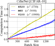
(a)

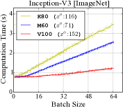
(b)

Figure 4. The relationship between computation time and batch size of different GPU types.

3.3.2. A Drop-in Algorithm for LB-BSP in GPU Clusters

In this part, we devise a drop-in algorithm to iteratively approximate the equilibrium where the gap among all the workers’ batch processing time is minimized.

The whole batch size adjusting algorithm is elaborated in Alg. 2. After each training iteration, we identify two GPU workers: a leader—the GPU worker with the shortest batch processing time, and a straggler—the GPU worker with the longest batch processing time. If the leader has consecutively preceded the straggler during an observation window (observation window is introduced for robustness to non-deterministic random variations), we respectively increase (reduce) the leader (straggler)’s batch size by a certain amount called step size. Note that any GPU worker with less than 5% available memory would, to avoid OOM error, be excluded from being identified as the leader. Moreover, if with Alg. 2 a worker’s batch size is to be reduced below $0$, we should restart the training process without that worker, and the resultant setup is actually more efficient.

Moreover, to reduce resource wastage, the equilibrium should be approached efficiently with minimum oscillation. To this end, we introduce two phases: a fast-approach phase and a fine-tune phase. Initially the algorithm enters the fast-approach phase, where we set a relatively large step size and short observation window; then, once oscillation—a former leader now identified as a straggler or vice versa—is detected, we switch to the fine-tune phase by reducing the step size (e.g., to $1$) and increasing the observation window size.

Remarks. While Alg. 2 is designed for GPU clusters, it also applies to other accelerators like TPU or FPGA. Existing measurements have shown that TPU (Kochura et al., 2018) and FPGA (Posewsky and Ziener, 2018) also exhibit a non-linear, monotonically-increasing relationship between $t^{p}$ and $x$, making it feasible to adopt LB-BSP in heterogeneous clusters with those hardware.

Algorithm 2 Batch Size Updating in GPU Clusters

1:Input: {$x_{i}^{k-1}$}, {$t_{i}^{k-1}$}, {$m_{i}^{k}$} $\triangleright$ last batch size, last batch processing time & current GPU memory usage of all workers $(i\!=\!1,...,n)$

2:Require: past values of $\{t_{i}\},i=1,2,...n$;

3:        $\!\varDelta\!\leftarrow\!5$, $D\!\leftarrow\!5$ $\triangleright$ $\varDelta$: step size; $D$: observation window size

4:procedure GPU_UpdateBatchSize($k$)

5:    leader $\leftarrow$ $\arg\min_{i}\{t_{i}^{k-1}\mid m_{i}^{k}\leq 0.95\}$

6:    straggler $\leftarrow$ $\arg\max_{i}\{t_{i}^{k-1}\}$

7:    $x_{i}^{k}\leftarrow x_{i}^{k-1},i=1,2,...,n$

8:    if $x_{\text{{straggler}}}^{k-1}\leq\varDelta$ then

9:         return {$x_{i}^{k}$} $\triangleright$ print warning: remove this straggler!     

10:    if $\forall h\in\{k-D,...,k-1\},t_{\text{{leader}}}^{h}<t_{\text{{straggler}}}^{h}$ then

11:        $x_{\text{{leader}}}^{k}\leftarrow x_{\text{{leader}}}^{k-1}+\varDelta$ ; $x_{\text{{straggler}}}^{k}\leftarrow x_{\text{{straggler}}}^{k-1}-\varDelta$

12:    else if $\exists h\in\{1,...,k-1\},t_{\text{{leader}}}^{h}>t_{\text{{straggler}}}^{h}$ then

13:        $\varDelta\leftarrow 1$, $D\leftarrow 20$ $\triangleright$ switch to fine-tune phase     return {$x_{i}^{k}$}

3.4. Weighted Gradient Aggregation

By tuning the worker batch size with Alg. 1 and Alg. 2, we can effectively eliminate deterministic stragglers and achieve high hardware efficiency. Yet, the resultant batch sizes on different workers would be inconsistent, which may affect the statistical efficiency. In this part, we first elaborate that problem and then give our solution.

Problem of Naive Aggregation under LB-BSP. Under BSP, the aggregated global gradient $g$ for parameter updating is the naive average of the gradients from all the workers. Suppose there are $n$ workers and $g_{i}$ is the gradient calculated on worker-$i$ ($i$=$1,2,...,n$), then

(5) $$g=\frac{1}{n}\sum_{i=1}^{n}g_{i},\textnormal{ where }g_{i}=\frac{1}{|B_{i}|}\sum_{s\in B_{i}}{\nabla l(s,\omega)}.$$

Here $B_{i}$ is the batch on worker-$i$. Getting rid of $g_{i}$, we have

(6) $$g=\frac{1}{n}\sum_{i=1}^{n}\frac{1}{|B_{i}|}\sum_{s\in B_{i}}{\nabla l(s,\omega)}=\sum_{i=1}^{n}\sum_{s\in B_{i}}{\frac{1}{n|B_{i}|}\!\!\cdot\!\nabla l(s,\omega)}.\!$$

This implies that, when workers have different batch sizes ($|B_{i}|$), the significance of different samples, i.e., $\frac{1}{n|B_{i}|}$, is also different. Thus $g$ is biased to samples in small batches, which may harm the statistical efficiency. To verify that, we train the Inception-V3 model under Alg. 2 in a 16-node heterogeneous GPU cluster (i.e., Cluster-A in section 5.1). After traversing the ImageNet dataset for 20 epochs, the training accuracy only reaches 43%, much worse than that under BSP (59%).

Weighted Gradient Aggregation. To avoid biased gradient, we propose weighted gradient aggregation—using a worker’s batch size as the weight when aggregating gradients. Suppose the total batch size is $\sum\nolimits_{j=1}^{n}{|B_{j}|}\!=\!\!X$, then we have

(7) $$g=\frac{1}{\sum\nolimits_{j=1}^{n}{|B_{j}|}}\sum_{i=1}^{n}{|B_{i}|\cdot g_{i}}=\sum_{i=1}^{n}\sum_{s\in B_{i}}{\frac{1}{X}\cdot\nabla l(s,\omega)}.$$

Obviously, now each sample plays an equal role in parameters updating, regardless of the batch size inconsistency. After that fix, for i.i.d. dataset, i.e., samples being independent and identically distributed, LB-BSP can achieve identical statistical efficiency with BSP, which is known to be optimal.

3.5. Discussion on Data Access Frequency

In this paper, we focus on cases where each worker can access the entire dataset via local storage or Network File System (NFS) (Shvachko et al., 2010; glu, 2020; Schmuck and Haskin, 2002). In shared production clusters, it has become almost a norm to store data in NFS (the access delay can be made negligible via pre-fetching), which largely facilitates data management and job migration (Hazelwood et al., 2018; Jeon et al., 2018; Xiao et al., 2018; Gu et al., 2019).

Nonetheless, there may still exist some cases that each worker can only access a local partition of the training dataset. Under LB-BSP where faster workers iterate with larger batches, this means that samples on faster workers would be accessed more frequently. Such a problem of uneven sample access frequency may lead to inaccurate training results, especially when the dataset is not well shuffled before being partitioned and there are huge gaps on worker processing capability. To address uneven sample access frequency with transparency to the upper level training process, we suggest an iterative SSP-style data scheduling scheme: once the traversal times of one partition exceed another over a given threshold, we launch a background process to migrate certain amount of samples from the slower worker to the faster one. We have prototyped this method atop PyTorch, and verified that it could make ideal accuracy even under non-i.i.d. data distribution. Such a kind of data migration method is indeed light-weight in GPU clusters, because in GPU clusters the worker speed is relatively stable and data migration is done-once-and-working-forever, with the overhead amortized.

4. Implementation

Algorithm 3 LB-BSP Workflow

1:Worker: i=1, 2, …, n:

2:procedure WorkerIterate($k$)

3:    $x_{i}\!\leftarrow\!$ BatchSizeManager.UpdateBatchSize($<$states$>$)

4:$\triangleright$ blocking in CPU clusters and non-blocking in GPU clusters

5:    load the next data batch $B_{i}^{k}$ such that $|B_{i}^{k}|=x_{i}$

6:    pull $w^{k}$ from PS

7:    calculate local gradient $g_{i}^{k}$

8:    push $\bar{g}_{i}^{k}\leftarrow\frac{nx_{i}}{X}g_{i}^{k}$ to PS $\triangleright$ $\bar{g}_{i}^{k}$: weighted gradient

1:Parameter Server (PS):

2:procedure ParameterServerIterate($k$)

3:    aggregate gradient $g^{k}$ $\leftarrow$$\frac{1}{n}\sum_{i=1}^{n}\bar{g}_{i}^{k}=\frac{1}{X}\sum_{i=1}^{n}|B_{i}^{k}|g_{i}^{k}$

4:    update parameters $w^{k+1}$ $\leftarrow$ $w^{k}-\eta g^{k}$ $\triangleright$ $\eta$: learning rate

1:BatchSizeManager:

2:procedure UpdateBatchSize($<$states$>$)

3:    Refer to Alg. 1 (CPU cluster) or Alg. 2 (GPU cluster).

We implement LB-BSP with BatchSizeManager, a Python module that can be integrated into existing ML frameworks including TensorFlow (Abadi et al., 2016), PyTorch (PyT, 2020) and MXNet (Chen et al., 2015).

Architecture Overview. The overall workflow of LB-BSP is described in Alg. 3 and Fig. 5. In the beginning of iteration $k$, each worker pushes its latest execution information ($\langle$ batch processing time $t^{k-1}$, CPU usage $c^{k}$, memory usage $m^{k}$ $\rangle$ for CPU clusters, or $\langle t^{k-1}$, $m^{k}\rangle$ for GPU clusters) to the BatchSizeManager, and then pulls back the updated batch size $x^{k}$. Note that LB-BSP is also applicable if the gradients are aggregated with the All-Reduce architecture.

In particular, for CPU clusters the batch size updating process is blocking so that the BatchSizeManager can get the latest state information for speed prediction; yet for GPU clusters, it is non-blocking because GPU workers’ state is more stable (section 3.3), and non-blocking interaction can avoid prolonging the very short GPU iterations. To that end, on each GPU worker we launch a separate thread to update batch size in the background.

Enabling Variable Batch Size. In existing ML frameworks, batch size is set as a constant when defining the computation graph, with no direct APIs to configure it during the training process. To enable variable batch size, in TensorFlow we decouple the batch size from the symbolic dataflow graph, and specify it as a tensor value passed to TensorFlow session through the feed_dict API. For MXNet and PyTorch, we respectively customize the DataIter and BatchSampler so that they can accept a user-specified batch size at runtime and generate a corresponded sample batch.

Measuring Worker Execution Status. To implement LB-BSP, at the worker side, we need to obtain the batch processing time $t$ and state information (e.g., CPU or memory usage). Acquiring $t$ is easy in dynamic-graph based frameworks like PyTorch, but is challenging for static-graph based frameworks like TensorFlow or MXNet. In TensorFlow, each iteration (forward or backward propagation and synchronization) is executed as a whole with tf.Session(), which cannot be decomposed with simple instructions. We choose to profile the batch processing time from the Timeline log once each iteration finishes. Instead of respectively measuring the communication time and computation time which might overlap with each other, we directly calculate batch processing time as the iteration time minus the synchronization waiting time (i.e., duration of the sync_token_q_Dequeue operation). Besides, to measure the CPU or memory usage we resort to the Python psutil (psu, 2020) library, and to measure the GPU memory usage we adopt the tf.contrib.memory_stats.BytesInUse() operation.

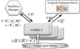
(a)

Figure 5. LB-BSP workflow in iteration $k$ (the circled numbers represent the execution order). The logical PS can be in the form of distributed shards, or be replaced by the All-Reduce architecture.

Thrift RPC Protocol. The BatchSizeManager can be located in a dedicated machine or co-located with the PS process on an existing server of the cluster. For efficient communication between the BatchSizeManager and workers, we employ Apache Thrift (thr, 2020), a lightweight RPC protocol developed by Facebook, and we create a thread pool to serve the worker requests in parallel.

Online NARX Training. The NARX models we use for CPU clusters are written in Keras (Ker, 2020), a high-level neural network API. Accurate NARX training requires collecting enough samples, so we enable NARX prediction only after the first $500$ iterations. In practice we find that $500$ samples are enough for accurately training our NARX models, which are quite simple (section 3.2.2). Within the first $500$ iterations, we can use EMA or, if that training job is recurring, the past NARX models trained in former runs. For fast convergence, we initialize NARX models by model reusing (Yang et al., 2017)—with the models trained even for other workers or ML jobs. Besides, we also adopt early stopping (Yao et al., 2007) and in practice we found that most training processes terminate within 10 steps.

5. Evaluation

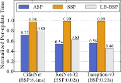
(a) Hardware Efficiency

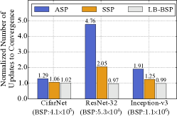
(b) Statistical Efficiency

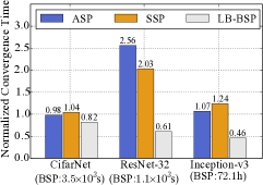
(c) Overall Convergence Efficiency

Figure 6. Training efficiency under different worker coordination schemes in Cluster-A.

In this section we systematically evaluate the performance of LB-BSP in non-dedicated clusters. We start with the end-to-end (section 5.1) and micro-benchmark (section 5.2) evaluations in GPU clusters. Then we resort to model training with leftover resources in production CPU clusters (section 5.3), with a deep dive analysis of the NARX prediction approach (section 5.4). Finally we evaluate the overhead of our LB-BSP solution in section 5.5.

5.1. End-to-End Result in GPU Cluster

Experimental Setup. As elaborated in section 2.1, there do exist some scenarios (e.g., due to budget limitation or fairness policy) where model training has to be conducted in heterogeneous GPU clusters. To emulate such scenarios, we build Cluster-A, a heterogeneous GPU cluster with 16 Amazon EC2 instances: four p3.2xlarge instances (each with one Tesla V100 GPU), four g3.4xlarge instances (each with one Tesla M60 GPU), four p2.xlarge instances (each with one Tesla K80 GPU), and four g2.2xlarge instances (each with one GRID K520 GPU). On each instance we run a worker process and a collocated PS shard under TensorFlow 1.4.0.

With Cluster-A, we train the CifarNet (Krizhevsky and Hinton, 2009) and ResNet-32 (He et al., 2016) model on CIFAR-10 dataset, and Inception-V3 (Szegedy et al., 2016) model on ImageNet dataset (Russakovsky et al., 2015) (containing 1.28 million of training images of 1000 classes). For simplicity each worker locally hosts a full dataset copy. The initial batch size of each worker is set to $128$ for CIFAR-10, and $32$ for ImageNet. The initial learning rate is set to $0.01$. The schemes evaluated in this part are BSP, ASP, SSP and LB-BSP, and we defer the comparisons with FlexRR and redundant execution to CPU clusters. We measure the overall training efficiency as well as the hardware and statistical efficiency. The results are summarized in Fig. 6, where BSP is the baseline and all the values displayed are normalized by that under BSP.

Hardware Efficiency. The metric we use for hardware efficiency is per-update time—the average time it takes for the PS to receive one gradient update. For BSP and LB-BSP, per-update time is the average iteration time divided by the number of workers. Fig. 6a shows that LB-BSP remarkably outperforms BSP and SSP, and this is consistent with our analysis in section 2.2. Interestingly, LB-BSP is even $15\%$ better than ASP in hardware efficiency when training Inception-V3 —we will explain that with micro-benchmark evaluations in section 5.2.

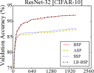
(a)

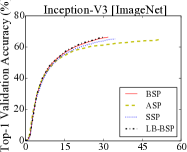
(b)

Figure 7. Test accuracy against training epochs.

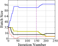
(a)

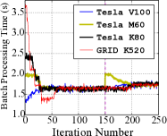
(b)

Figure 8. Instantaneous batch size and batch processing time of the four heterogeneous GPU workers under LB-BSP. At iteration $30$, Alg. 2 enters the fine-tune phase, and batch sizes of the four workers stabilize at $(89,21,12,6)$. Later at iteration 150, bandwidth of the M60 GPU worker is reduced to emulate a migration-caused locality degradation, and the four workers then enter a new equilibrium.

Statistical Efficiency. Statistical efficiency is measured as the number of updates required to reach the target accuracy. We set different near-optimal accuracy targets for different models: $0.80$ for CifarNet, $0.86$ for ResNet-32, and $0.65$ for Inception-V3. As shown in Fig. 6b, for each model under LB-BSP, the number of updates required to reach the target accuracy is almost identical with that under BSP. In contrast, ASP and SSP require up to $4.76\times$ and $2.05\times$ the number of BSP to make that accuracy.

Moreover, ASP and SSP fall behind not only in the convergence speed, but also in the the ultimate accuracy attained. Fig. 7 shows the convergence curves of ResNet-32 and Inception-V3, where an epoch is a full pass of all the samples in the CIFAR-10 or ImageNet dataset. For ResNet-32, we find that the accuracy made by ASP or SSP gets stuck below $0.88$, while BSP and LB-BSP successfully make the ideal accuracy of $0.92$. Also, for Inception-V3, BSP and LB-BSP already surpass ASP and SSP even for reaching a sub-optimal accuracy target $0.65$.

Instance Type	CPU, Mem (core, GiB)	Num
m4.2xlarge	(8, 32)	17
c5.2xlarge	(8, 16)	10
r4.2xlarge	(8, 61)	2
m4.4xlarge	(16, 64)	2
m4.xlarge	(4, 16)	1

Table 2. Cluster-B composition.

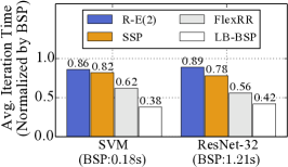
(a)

Figure 9. Iteration time with different schemes in Cluster-B.

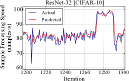
Figure 10. NARX prediction result on an m4.2xlarge instance.

Overall Convergence Efficiency. Fig. 6c shows the overall time required to reach the target accuracy, where LB-BSP surpasses the second best by up to $54\%$. Therefore, it’s highly rewarding to employ LB-BSP in such heterogeneous GPU clusters. We further train ResNet-32 in a 12-node GPU cluster without the p3.2xlarge instances, and the iteration speedup of LB-BSP over BSP reduces (from $37\%$ in Fig. 6a) to $28\%$. Thus, the more heterogeneous the cluster is, the more necessary it is to adopt LB-BSP for load balancing.

5.2. Micro-benchmark in GPU Cluster

To further understand LB-BSP behavior from the micro level, we scale down Cluster-A to contain only 4 GPU instances each of a distinct type, and measure the instantaneous worker batch size and batch processing time when training Inception-V3. As shown in Fig. 8, LB-BSP gradually increases the batch size of the most powerful worker (i.e., the one with the Tesla V100 GPU), with the batch sizes of the other workers correspondingly decreased. Finally an equilibrium is reached where all the workers share almost the same batch processing time. Note that after iteration $30$, the LB-BSP algorithm (Alg. 2) enters the fine-tune phase, where the batch sizes of the four workers gradually stabilize at $(89,21,12,6)$.

Fig. 8 also helps to elaborate why LB-BSP can even outperform ASP in hardware efficiency. By yielding 26 samples (from 32 to 6), the worker with K520 GPU has its batch processing time reduced by nearly 2s; in contrast, the worker with V100 GPU, after incorporating as many as 57 samples, only suffers an increase of 0.5s. Therefore, by allowing advanced workers to process more samples and achieve a higher utilization with negligible slowdown, LB-BSP can reduce the average cost to process one sample and improve the hardware efficiency.

Furthermore, we evaluate LB-BSP applicability in shared GPU clusters, and emulate the network variation caused by locality degradation when conducting cross-machine(rack) worker migration. In Fig. 8, at iteration 150 we bound the bandwidth of the worker with M60 GPU to 2.5Gbps (from EC2-provisioned 10Gbps, with the wondershaper (won, 2020) tool). The LB-BSP algorithm learns that shortly and then gradually adjusts workers’ batch size to reach another equilibrium. This confirms that LB-BSP can work well in multi-tenant GPU clusters with job migrations from time to time.

5.3. Evaluation in Shared CPU Cluster

Experimental Setup. As elaborated in section 3.2, non-neural-network or not-so-urgent models may be trained in non-dedicated CPU clusters. To evaluate LB-BSP performance in such scenarios, we manually created Cluster-B, a heterogeneous CPU cluster that emulates the shared production environment where ML models are trained with the dynamic leftover resources  (Reiss et al., 2012; Cortez et al., 2017; Li et al., 2018; Hazelwood et al., 2018). Cluster-B is built based on a one-hour snapshot of Google Trace (Reiss et al., 2012). That trace discloses the machine configurations (CPU/Memory capacities in normalized form) of a production cluster from Google, together with the information of all the involved jobs/tasks during a selected month—including their resource consumptions and start/end times.

More specifically, we scale down the totally 12,583 machines to 32 EC2 instances, with the former’s hardware heterogeneity proportionally preserved—by accordingly selecting the instance types and the quantity of each type, as summarized in Table 2. Meanwhile, resource dynamicity of that Google cluster is also emulated: we randomly map each instance to a machine in the Google cluster, and launch a set of faked tasks sharing identical behaviors (i.e., start/end times & CPU/memory consumptions) with those submitted to that Google machine.

Regarding the models, we train SVM on a malicious URL dataset (Ma et al., 2009), and ResNet-32 on CIFAR-10 dataset. The batch size for SVM training is $10\%$ of the whole URL dataset (as in (Jiang et al., 2017)), and is 128 for ResNet-32.

The schemes evaluated are Redundant Execution (R-E), SSP, LB-BSP and FlexRR. The first three schemes are implemented in TensorFlow. For R-E, we add two c5.2xlarge instances (also in resource contention with some faked tasks) to Cluster-B as the backup worker, and only collect $32$ gradients returned the earliest in each iteration. R-E is supported in TensorFlow with the replicas_to_aggregate parameter. In SSP, the bound of iteration gap is still set to $5$, as in section 5.1. Regarding FlexRR, since it is not open-sourced and its sequential sample processing manner is not supported in current ML frameworks (section 2.2.3), we choose to emulate it in PyTorch. We generate tiny batches each containing only one sample, and then encapsulate them into logical batches of designated size; such a logical batch can then be processed in a sequential manner. Meanwhile, each worker’s helper group is set to be all the remaining workers, and for the other setups (e.g., progress check frequency, trigger condition of load reassignment), we follow the suggested values in (Harlap et al., 2016).

Hardware Efficiency. Fig. 10 shows the average iteration time when training SVM and ResNet-32 under different schemes in Cluster-B. For fair comparison, each value in Fig. 10 is normalized by the BSP performance in the corresponded framework (sequential-processing-style PyTorch for FlexRR, and TensorFlow for the others). As in Fig. 10, R-E and SSP speed up the training iterations only marginally, because they focus on either worst-case or transient stragglers, but the stragglers in Cluster-B span a wide range of degrees and durations. Meanwhile, regarding FlexRR, its performance is better but not the best, because its decentralized load balancing decisions are not optimal, and meanwhile it suffers non-negligible measurement, negotiation and load reassignment overheads (section 2.2.3). In contrast, LB-BSP can bring a speedup of $62\%$ for SVM and $58\%$ for ResNet-32 over BSP, outperforming the second best (FlexRR) by up to 38.7%. Thus, given that LB-BSP can also make the optimal statistical efficiency (section 5.1), it can surely lead to the best convergence efficiency among all the schemes evaluated.

5.4. NARX Performance Deep Dive

Method	Configuration	RMSE	Avg. Iteration Time (Normalized by BSP)
Memoryless	-	11.85	$0.58$
EMA	$\alpha$=0.2	7.85	$0.48$
ARIMA	($p$,$d$,$q$)=(2,2,1)	9.67	0.52
SimpleRNN	look-back=2	8.34	0.49
LSTM	look-back=2	9.19	0.51
NARX	look-back=2	4.78	0.42

Table 3. RMSE and iteration speedup when applying different prediction approaches in LB-BSP.

In this part, we further evaluate the prediction performance of the NARX model (section 3.2.2) we use in Cluster-B.

Visual Analysis. To get a visual understanding of the NARX prediction performance, we randomly select a period (iteration 1200$\sim$1300) from the ResNet-32 training process on one m4.2xlarge instance of Cluster-B; the actual and predicted sample processing speeds are presented in Fig. 10. From it we observe that the benefit of NARX is twofold. On the one hand, NARX is robust to non-deterministic transient perturbations: when there are “spikes” (like the sharp wave around iteration 1206) in the actual speed curve, the predicted curve fluctuates much less. This is because NARX predicts also with the worker’s available memory and CPU amounts, which are relatively stable during those “spikes”. On the other hand, when the actual speed increases not for randomness but for non-transient deterministic factors like increased CPU or memory resources (e.g., around iteration 1270), the predicted speed can promptly catch up.

Comparison with Other Approaches. We further compare NARX with other approaches surveyed in section 3.2.2, as listed in Table 3. The memoryless method means to take last iteration’s sample processing speed as the predicted one. Regarding the EMA approach, the smoothing factor $\alpha$ (weight of the latest observation) is set to be $0.2$. As for the statistical prediction approach—ARIMA, its order of the autoregressive model ($p$), degree of differencing ($d$), and order of the moving average ($q$) are respectively set to 2, 2 and 1, based on the model selection techniques (Ozaki, 1977). Finally, for SimpleRNN (plain RNN) and LSTM, their look-back window size is set to 2, the same as in NARX.

Then, we replace the NARX approach with those candidate prediction approaches, and re-train ResNet-32 model under LB-BSP in Cluster-B. For each approach, we record the average root-mean-square error (RMSE) of the prediction results and the corresponded iteration time (normalized by the iteration time under BSP). From Table 3, the NARX approach, with the ability to perceive CPU/memory resource variations, attains the best performance—it surpasses the second best by around $40\%$ in RMSE and $15\%$ in average iteration time.

5.5. System Overhead and Scalability

In TensorFlow, LB-BSP introduces two extra procedures: first to extract batch processing time from execution logs (e.g., the Timeline object), and second to conduct RPC communication between the BatchSizeManager and workers. Yet, they won’t slow down GPU workers because of our non-blocking design (section 4), and here we measure the slowdown caused by those two extra procedures in CPU clusters.

We respectively train ResNet-32 and Inception-V3 model for 1000 iterations in three CPU clusters—a homogeneous cluster with 33 c5.2xlarge instances (32 worker nodes and 1 separate node hosting both the PS and BatchSizeManager), and then its enlarged version with a doubled/tripled number of workers. Fig. 11 shows the average time respectively spent on log processing and batch size updating, normalized by the iteration time (error bars show the $5^{th}$/$95^{th}$ percentile). Even in the largest cluster with 96 workers, the total overheads are less than 1.1% of the iteration time for both models. This indirectly confirms that, performance of the PS is almost not affected by the co-located BatchSizeManger.

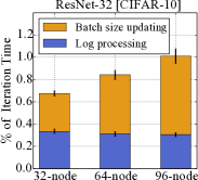
(a)

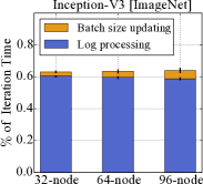
(b)

Figure 11. LB-BSP overheads in CPU clusters.

6. Additional Related Work

Besides the related work in section 2.2, in this part we discuss some additional related work on batching. Batching is necessary when processing long-lasting streaming inputs or training models with large datasets. For big data streaming systems (Zaharia et al., 2013; Toshniwal et al., 2014), some works (Das et al., 2014; Zhang et al., 2016) have explored how to adaptively adjust the batching interval when faced with dynamic data rates or operating conditions. For iterative model training, some (Devarakonda et al., 2017; De et al., 2017) have proposed to adaptively increase batch size during the training process to yield faster convergence. Yet, those works don’t involve workload allocation among parallel workers, and are thus orthogonal to LB-BSP.

7. Conclusion

In this work, we propose LB-BSP to load-balance distributed model training workloads in a semi-dynamic manner, by speculatively apportioning the load on the workers according to their temporal processing capability. LB-BSP is tailor-made respectively for both CPU and GPU clusters, and our experiments on Amazon EC2 have shown clear evidence that it can effectively eliminate stragglers in non-dedicated clusters, speeding up model convergence by over $50\%$.

References

- (1)
- str (2019) 2019. Stress-ng: a tool to load and stress a computer system. http://manpages.ubuntu.com/manpages/artful/man1/stress-ng.1.html.
- gpu (2019) 2019. Train Deep Learning Models on GPUs using Amazon EC2 Spot Instances. https://aws.amazon.com/en/blogs/machine-learning/train-deep-learning-models-on-gpus-using-amazon-ec2-spot-instances/.
- thr (2020) 2020. Apache Thrift. https://thrift.apache.org/.
- ec2 (2020) 2020. EC2 Spot Instances. https://aws.amazon.com/ec2/spot/.
- flo (2020) 2020. FloydHub. https://floydhub.com/.
- glu (2020) 2020. GlusterFS. https://docs.gluster.org/en/latest/.
- Ker (2020) 2020. Keras. https://keras.io/.
- psu (2020) 2020. Python Psutil. https://psutil.readthedocs.io/en/latest/.
- PyT (2020) 2020. PyTorch. https://pytorch.org/.
- won (2020) 2020. Wonder Shaper. https://github.com/magnific0/wondershaper.
- Abadi et al. (2016) Martín Abadi et al. 2016. TensorFlow: A System for Large-Scale Machine Learning. In USENIX OSDI.
- Acar et al. (2013) Umut A Acar, Arthur Charguéraud, and Mike Rainey. 2013. Scheduling parallel programs by work stealing with private deques. In ACM SIGPLAN Notices.
- Acun and Kale (2016) Bilge Acun and Laxmikant V Kale. 2016. Mitigating processor variation through dynamic load balancing. In IEEE IPDPSW.
- Al Nuaimi et al. (2012) Klaithem Al Nuaimi, Nader Mohamed, Mariam Al Nuaimi, and Jameela Al-Jaroodi. 2012. A survey of load balancing in cloud computing: Challenges and algorithms. In IEEE NCA.
- Ananthanarayanan et al. (2013) Ganesh Ananthanarayanan, Ali Ghodsi, Scott Shenker, and Ion Stoica. 2013. Effective Straggler Mitigation: Attack of the Clones.. In USENIX NSDI.
- Argyropoulos et al. (2016) Dimitrios Argyropoulos, Dimitris S Paraforos, Rainer Alex, Hans W Griepentrog, and Joachim Müller. 2016. NARX neural network modelling of mushroom dynamic vapour sorption kinetics. IFAC-PapersOnLine 49, 16 (2016), 305–310.
- Blumofe and Leiserson (1999) Robert D Blumofe and Charles E Leiserson. 1999. Scheduling multithreaded computations by work stealing. JACM 46, 5 (1999), 720–748.
- Cadenas et al. (2016) Erasmo Cadenas, Wilfrido Rivera, Rafael Campos-Amezcua, and Roberto Cadenas. 2016. Wind speed forecasting using the NARX model, case: La Mata, Oaxaca, México. Neural Computing and Applications 27, 8 (2016), 2417–2428.
- Chaudhary et al. (2020) Shubham Chaudhary, Ramachandran Ramjee, Muthian Sivathanu, Nipun Kwatra, and Srinidhi Viswanatha. 2020. Balancing efficiency and fairness in heterogeneous GPU clusters for deep learning. Proceedings of the Fifteenth European Conference on Computer Systems (2020).
- Chen et al. (2016) Jianmin Chen, Rajat Monga, Samy Bengio, and Rafal Jozefowicz. 2016. Revisiting distributed synchronous SGD. arXiv preprint arXiv:1604.00981 (2016).
- Chen et al. (2015) Tianqi Chen, Mu Li, Yutian Li, Min Lin, Naiyan Wang, Minjie Wang, Tianjun Xiao, Bing Xu, Chiyuan Zhang, and Zheng Zhang. 2015. Mxnet: A flexible and efficient machine learning library for heterogeneous distributed systems. arXiv preprint arXiv:1512.01274 (2015).
- Chilimbi et al. (2014) Trishul Chilimbi, Yutaka Suzue, Johnson Apacible, and Karthik Kalyanaraman. 2014. Project adam: Building an efficient and scalable deep learning training system. In USENIX OSDI.
- Collobert et al. (2011) Ronan Collobert, Jason Weston, Léon Bottou, Michael Karlen, Koray Kavukcuoglu, and Pavel Kuksa. 2011. Natural language processing (almost) from scratch. J. Mach. Learn. Res. 12, Aug (2011), 2493–2537.
- Connor et al. (1994) Jerome T Connor, R Douglas Martin, and Les E Atlas. 1994. Recurrent neural networks and robust time series prediction. IEEE Trans. on Neural Networks 5, 2 (1994), 240–254.
- Cortez et al. (2017) Eli Cortez, Anand Bonde, Alexandre Muzio, Mark Russinovich, Marcus Fontoura, and Ricardo Bianchini. 2017. Resource Central: Understanding and Predicting Workloads for Improved Resource Management in Large Cloud Platforms.
- Cui et al. (2014) Henggang Cui, James Cipar, Qirong Ho, Jin Kyu Kim, Seunghak Lee, Abhimanu Kumar, Jinliang Wei, Wei Dai, Gregory R Ganger, Phillip B Gibbons, et al. 2014. Exploiting Bounded Staleness to Speed Up Big Data Analytics. In USENIX ATC.
- Cui et al. (2016) Henggang Cui, Hao Zhang, Gregory R Ganger, Phillip B Gibbons, and Eric P Xing. 2016. GeePS: Scalable deep learning on distributed gpus with a gpu-specialized parameter server. In ACM Eurosys.
- Das et al. (2014) Tathagata Das, Yuan Zhong, Ion Stoica, and Scott Shenker. 2014. Adaptive stream processing using dynamic batch sizing. In ACM SoCC.
- De et al. (2017) Soham De, Abhay Yadav, David Jacobs, and Tom Goldstein. 2017. Automated inference with adaptive batches. In Artificial Intelligence and Statistics. 1504–1513.
- Dean et al. (2012) Jeffrey Dean, Greg Corrado, Rajat Monga, Kai Chen, Matthieu Devin, Mark Mao, Andrew Senior, Paul Tucker, Ke Yang, Quoc V Le, and Andrew Ng. 2012. Large scale distributed deep networks. In NIPS.
- Dean and Ghemawat (2010) Jeffrey Dean and Sanjay Ghemawat. 2010. MapReduce: a flexible data processing tool. Commun. ACM 53, 1 (2010), 72–77.
- Devarakonda et al. (2017) Aditya Devarakonda, Maxim Naumov, and Michael Garland. 2017. AdaBatch: Adaptive Batch Sizes for Training Deep Neural Networks. arXiv preprint arXiv:1712.02029 (2017).
- Diaconescu (2008) Eugen Diaconescu. 2008. The use of NARX neural networks to predict chaotic time series. Wseas Transactions on computer research 3, 3 (2008), 182–191.
- Dinan et al. (2009) James Dinan, D Brian Larkins, Ponnuswamy Sadayappan, Sriram Krishnamoorthy, and Jarek Nieplocha. 2009. Scalable work stealing. In IEEE/ACM SC.
- Ediger and Akar (2007) Volkan Ş Ediger and Sertac Akar. 2007. ARIMA forecasting of primary energy demand by fuel in Turkey. Energy Policy 35, 3 (2007), 1701–1708.
- Farabet et al. (2013) Clement Farabet, Camille Couprie, Laurent Najman, and Yann LeCun. 2013. Learning hierarchical features for scene labeling. IEEE Trans. Pattern Anal. Mach. Intell. 35, 8 (2013), 1915–1929.
- Gao and Er (2003) Yang Gao and Meng Joo Er. 2003. NARMAX-model-based time series modeling and prediction: feedforward and recurrent fuzzy neural network approaches. In WSEAS CSECS.
- Goyal et al. (2017) Priya Goyal, Piotr Dollár, Ross Girshick, Pieter Noordhuis, Lukasz Wesolowski, Aapo Kyrola, Andrew Tulloch, Yangqing Jia, and Kaiming He. 2017. Accurate, Large Minibatch SGD: Training ImageNet in 1 Hour. arXiv preprint arXiv:1706.02677 (2017).
- Gu et al. (2019) Juncheng Gu, Mosharaf Chowdhury, Kang G Shin, Yibo Zhu, Myeongjae Jeon, Junjie Qian, Hongqiang Liu, and Chuanxiong Guo. 2019. Tiresias: A GPU Cluster Manager for Distributed Deep Learning. In USENIX NSDI.
- Gu et al. (2017) Jiazhen Gu, Huan Liu, Yangfan Zhou, and Xin Wang. 2017. DeepProf: Performance Analysis for Deep Learning Applications via Mining GPU Execution Patterns. arXiv preprint arXiv:1707.03750 (2017).
- Harlap et al. (2016) Aaron Harlap, Henggang Cui, Wei Dai, Jinliang Wei, Gregory R Ganger, Phillip B Gibbons, Garth A Gibson, and Eric P Xing. 2016. Addressing the straggler problem for iterative convergent parallel ML. In ACM SoCC.
- Hazelwood et al. (2018) Kim Hazelwood, Sarah Bird, David Brooks, Soumith Chintala, Utku Diril, Dmytro Dzhulgakov, Mohamed Fawzy, Bill Jia, Yangqing Jia, Aditya Kalro, et al. 2018. Applied Machine Learning at Facebook: A Datacenter Infrastructure Perspective. In IEEE HPCA.
- He et al. (2016) Kaiming He, Xiangyu Zhang, Shaoqing Ren, and Jian Sun. 2016. Deep residual learning for image recognition. In IEEE CVPR.
- Ho et al. (2013) Qirong Ho, James Cipar, Henggang Cui, Seunghak Lee, Jin Kyu Kim, Phillip B Gibbons, Garth A Gibson, Greg Ganger, and Eric P Xing. 2013. More effective distributed ML via a stale synchronous parallel parameter server. In NIPS.
- Hochreiter and Schmidhuber (1997) Sepp Hochreiter and Jürgen Schmidhuber. 1997. Long short-term memory. Neural computation 9, 8 (1997), 1735–1780.
- Jeon et al. (2018) Myeongjae Jeon, Shivaram Venkataraman, Junjie Qian, Amar Phanishayee, Wencong Xiao, and Fan Yang. 2018. Multi-tenant GPU Clusters for Deep Learning Workloads: Analysis and Implications. MSR Technical Report 2018-13 (2018).
- Jia et al. (2018) Xianyan Jia, Shutao Song, Wei He, Yangzihao Wang, Haidong Rong, Feihu Zhou, Liqiang Xie, Zhenyu Guo, Yuanzhou Yang, Liwei Yu, et al. 2018. Highly Scalable Deep Learning Training System with Mixed-Precision: Training ImageNet in Four Minutes. arXiv preprint arXiv:1807.11205 (2018).
- Jia et al. (2014) Yangqing Jia, Evan Shelhamer, Jeff Donahue, Sergey Karayev, Jonathan Long, Ross Girshick, Sergio Guadarrama, and Trevor Darrell. 2014. Caffe: Convolutional architecture for fast feature embedding. In ACM Multimedia.
- Jiang et al. (2017) Jiawei Jiang, Bin Cui, Ce Zhang, and Lele Yu. 2017. Heterogeneity-aware distributed parameter servers. In ACM SIGMOD.
- Kochura et al. (2018) Yuriy Kochura, Yuri Gordienko, Vlad Taran, Nikita Gordienko, Alexandr Rokovyi, Oleg Alienin, and Sergii Stirenko. 2018. Batch Size Influence on Performance of Graphic and Tensor Processing Units during Training and Inference Phases. arXiv preprint arXiv:1812.11731 (2018).
- Kokilavani et al. (2011) T Kokilavani, Dr DI George Amalarethinam, et al. 2011. Load balanced min-min algorithm for static meta-task scheduling in grid computing. International Journal of Computer Applications 20, 2 (2011), 43–49.
- Krizhevsky and Hinton (2009) Alex Krizhevsky and Geoffrey Hinton. 2009. Learning multiple layers of features from tiny images. Technical report, University of Toronto (2009).
- Krizhevsky et al. (2012) Alex Krizhevsky, Ilya Sutskever, and Geoffrey E Hinton. 2012. ImageNet classification with deep convolutional neural networks. In NIPS.
- Langford et al. (2009) John Langford, Alexander J Smola, and Martin Zinkevich. 2009. Slow learners are fast. In NIPS.
- Le et al. (2020) Tan Le, Xiao Shu Sun, Mosharaf Chowdhury, and Zhenhua Liu. 2020. AlloX: compute allocation in hybrid clusters. Proceedings of the Fifteenth European Conference on Computer Systems (2020).
- Li (2016) Ang Li. 2016. GPU performance modeling and optimization. Ph.D. Dissertation. Technische Universiteit Eindhoven.
- Li et al. (2014a) Mu Li, David G Andersen, Jun Woo Park, Alexander J Smola, Amr Ahmed, Vanja Josifovski, James Long, Eugene J Shekita, and Bor-Yiing Su. 2014a. Scaling Distributed Machine Learning with the Parameter Server. In USENIX OSDI.
- Li et al. (2014b) Mu Li, Tong Zhang, Yuqiang Chen, and Alexander J Smola. 2014b. Efficient mini-batch training for stochastic optimization. In ACM KDD.
- Li et al. (2018) Tian Li, Jie Zhong, Ji Liu, Wentao Wu, and Ce Zhang. 2018. Ease. ml: towards multi-tenant resource sharing for machine learning workloads. VLDB (2018).
- Lustig and Martonosi (2013) Daniel Lustig and Margaret Martonosi. 2013. Reducing GPU offload latency via fine-grained CPU-GPU synchronization. In IEEE HPCA.
- Ma et al. (2009) Justin Ma, Lawrence K Saul, Stefan Savage, and Geoffrey M Voelker. 2009. Identifying suspicious URLs: an application of large-scale online learning. In ACM ICML.
- Magni et al. (2014) Alberto Magni, Christophe Dubach, and Michael O’Boyle. 2014. Exploiting GPU hardware saturation for fast compiler optimization. In ACM GPGPU.
- Mahajan et al. (2020) Kshiteej Mahajan, Arjun Balasubramanian, Arjun Singhvi, Shivaram Venkataraman, Aditya Akella, Amar Phanishayee, and Shuchi Chawla. 2020. Themis: Fair and Efficient GPU Cluster Scheduling. In NSDI.
- Narayanan et al. (2020) Deepak Narayanan, Keshav Santhanam, Fiodar Kazhamiaka, Amar Phanishayee, and Matei Zaharia. 2020. Heterogeneity-Aware Cluster Scheduling Policies for Deep Learning Workloads. In USENIX OSDI.
- Ozaki (1977) T Ozaki. 1977. On the order determination of ARIMA models. Applied Statistics (1977), 290–301.
- Park et al. (2020) Jay H Park, Gyeongchan Yun, Chang M Yi, Nguyen T Nguyen, Seungmin Lee, Jaesik Choi, Sam H Noh, and Young-ri Choi. 2020. HetPipe: Enabling Large DNN Training on (Whimpy) Heterogeneous GPU Clusters through Integration of Pipelined Model Parallelism and Data Parallelism. In USENIX ATC.
- Peng et al. (2018) Yanghua Peng, Yixin Bao, Yangrui Chen, Chuan Wu, and Chuanxiong Guo. 2018. Optimus: an efficient dynamic resource scheduler for deep learning clusters. In ACM Eurosys.
- Polson and Sokolov (2017) Nicholas G Polson and Vadim O Sokolov. 2017. Deep learning for short-term traffic flow prediction. Transportation Research Part C: Emerging Technologies 79 (2017), 1–17.
- Posewsky and Ziener (2018) Thorbjörn Posewsky and Daniel Ziener. 2018. Throughput optimizations for FPGA-based deep neural network inference. Microprocessors and Microsystems 60 (2018), 151–161.
- Rather et al. (2015) Akhter Mohiuddin Rather, Arun Agarwal, and VN Sastry. 2015. Recurrent neural network and a hybrid model for prediction of stock returns. Expert Systems with Applications 42, 6 (2015), 3234–3241.
- Reiss et al. (2012) Charles Reiss, Alexey Tumanov, Gregory R Ganger, Randy H Katz, and Michael A Kozuch. 2012. Heterogeneity and dynamicity of clouds at scale: Google trace analysis. In ACM SoCC.
- Russakovsky et al. (2015) Olga Russakovsky, Jia Deng, Hao Su, Jonathan Krause, Sanjeev Satheesh, Sean Ma, Zhiheng Huang, Andrej Karpathy, Aditya Khosla, Michael Bernstein, Alexander C. Berg, and Li Fei-Fei. 2015. ImageNet Large Scale Visual Recognition Challenge. International Journal of Computer Vision (IJCV) 115, 3 (2015), 211–252. https://doi.org/10.1007/s11263-015-0816-y.
- Samal and Mishra (2013) Pooja Samal and Pranati Mishra. 2013. Analysis of variants in Round Robin Algorithms for load balancing in Cloud Computing. International Journal of computer science and Information Technologies 4, 3 (2013), 416–419.
- Schmuck and Haskin (2002) Frank B Schmuck and Roger L Haskin. 2002. GPFS: A Shared-Disk File System for Large Computing Clusters.. In USENIX FAST.
- Shvachko et al. (2010) Konstantin Shvachko, Hairong Kuang, Sanjay Radia, and Robert Chansler. 2010. The hadoop distributed file system. In IEEE MSST.
- Sutskever et al. (2014) Ilya Sutskever, Oriol Vinyals, and Quoc V Le. 2014. Sequence to sequence learning with neural networks. In NIPS.
- Szegedy et al. (2016) Christian Szegedy, Vincent Vanhoucke, Sergey Ioffe, Jon Shlens, and Zbigniew Wojna. 2016. Rethinking the inception architecture for computer vision. In IEEE CVPR.
- Tang and Chanson (2000) Xueyan Tang and Samuel T Chanson. 2000. Optimizing static job scheduling in a network of heterogeneous computers. In IEEE ICPP.
- Tantawi and Towsley (1985) Asser N Tantawi and Don Towsley. 1985. Optimal static load balancing in distributed computer systems. Journal of the ACM (JACM) 32, 2 (1985), 445–465.
- Toshniwal et al. (2014) Ankit Toshniwal, Siddarth Taneja, Amit Shukla, Karthik Ramasamy, Jignesh M Patel, Sanjeev Kulkarni, Jason Jackson, Krishna Gade, Maosong Fu, Jake Donham, et al. 2014. Storm@ twitter. In ACM SIGMOD.
- Xiao et al. (2018) Wencong Xiao, Romil Bhardwaj, Ramachandran Ramjee, Muthian Sivathanu, Nipun Kwatra, Zhenhua Han, Pratyush Patel, Xuan Peng, Hanyu Zhao, Quanlu Zhang, et al. 2018. Gandiva: introspective cluster scheduling for deep learning. In USENIX OSDI.
- Yang and He (2018) Jixiang Yang and Qingbi He. 2018. Scheduling parallel computations by work stealing: A survey. International Journal of Parallel Programming 46, 2 (2018), 173–197.
- Yang et al. (2017) Yang Yang, De-Chuan Zhan, Ying Fan, Yuan Jiang, and Zhi-Hua Zhou. 2017. Deep Learning for Fixed Model Reuse.. In AAAI. 2831–2837.
- Yao et al. (2007) Yuan Yao, Lorenzo Rosasco, and Andrea Caponnetto. 2007. On early stopping in gradient descent learning. Constructive Approximation 26, 2 (2007), 289–315.
- Zaharia et al. (2012) Matei Zaharia, Mosharaf Chowdhury, Tathagata Das, Ankur Dave, Justin Ma, Murphy McCauley, Michael J Franklin, Scott Shenker, and Ion Stoica. 2012. Resilient distributed datasets: A fault-tolerant abstraction for in-memory cluster computing. In USENIX NSDI.
- Zaharia et al. (2013) Matei Zaharia, Tathagata Das, Haoyuan Li, Timothy Hunter, Scott Shenker, and Ion Stoica. 2013. Discretized streams: Fault-tolerant streaming computation at scale. In ACM SOSP.
- Zaharia et al. (2008) Matei Zaharia, Andy Konwinski, Anthony D Joseph, Randy H Katz, and Ion Stoica. 2008. Improving MapReduce performance in heterogeneous environments.. In USENIX OSDI.
- Zhang et al. (2017a) Haoyu Zhang, Logan Stafman, Andrew Or, and Michael J Freedman. 2017a. SLAQ: quality-driven scheduling for distributed machine learning. In ACM SoCC.
- Zhang et al. (2017b) Hao Zhang, Zeyu Zheng, Shizhen Xu, Wei Dai, Qirong Ho, Xiaodan Liang, Zhiting Hu, Jinliang Wei, Pengtao Xie, and Eric P Xing. 2017b. Poseidon: An Efficient Communication Architecture for Distributed Deep Learning on GPU Clusters. In USENIX ATC.
- Zhang et al. (2016) Quan Zhang, Yang Song, Ramani R Routray, and Weisong Shi. 2016. Adaptive block and batch sizing for batched stream processing system. In IEEE ICAC.