Large scale classification in deep neural network with Label Mapping

Abstract

In recent years, deep neural network is widely used in machine learning. The multi-class classification problem is a class of important problem in machine learning. However, in order to solve those types of multi-class classification problems effectively, the required network size should have hyper-linear growth with respect to the number of classes. Therefore, it is infeasible to solve the multi-class classification problem using deep neural network when the number of classes are huge. This paper presents a method, so called Label Mapping (LM), to solve this problem by decomposing the original classification problem to several smaller sub-problems which are solvable theoretically. Our method is an ensemble method like error-correcting output codes (ECOC), but it allows base learners to be multi-class classifiers with different number of class labels. We propose two design principles for LM, one is to maximize the number of base classifier which can separate two different classes, and the other is to keep all base learners to be independent as possible in order to reduce the redundant information. Based on these principles, two different LM algorithms are derived using number theory and information theory. Since each base learner can be trained independently, it is easy to scale our method into a large scale training system. Experiments show that our proposed method outperforms the standard one-hot encoding and ECOC significantly in terms of accuracy and model complexity.

I Introduction

Deep learning has become one of the major research areas in the machine learning community. One of the challenge is that the structure of the deep network model is usually complicated. For general multi-class classification problems, the required parameters of the deep network need to have hyper-linear growth with respect to the class number. If the number of classes are large, the classification problem will become infeasible because the required resources for model computation and storage will be huge. However, today there are lots of applications that require to perform classification with huge number of classes, such as language model of word level, image recognition of shopping items in e-commerce (multi-billions of shopping items today in Taobao and Amazon), as well as handwriting recognition of 10K Chinese characters.

In fact, A general deep neural network classifier of $N$ classes can be treated as a series connection of a complex embedding in Euclidean space to the last but one layer, and a softmax classifier softmax$(Ax+b)$ of $N$ classes in the last layer. The complex embedding can be interpreted as a clustering process to cluster data based on their class labels, and the last layer tries to separate them. If the dimension of the Euclidean space in the last but one layer is bigger or equal to $N-1$, there exists a softmax classifier to separate those clusters with probability 1. But if the dimension of the Euclidean space in the last but one layer is less than $N-1$, there may exist a cluster where the center is inside the convex closure of the other cluster centers. In this case, there is no softmax classifier that can separate this cluster from other clusters, because a linear function on a convex set always take its maximal value at a vertex. (For a image, see Figure 2. For more detail, see section III.)

In order to solve the classification problems of $N$ classes with growing $N$, either the the dimension in the last but one layer is fixed, which leads to that the performance is bad, or the dimension in the last but one layer grow with the growing of $N$, which leads to that the parameter number in the last two layers grow hyper-linearly with the growing of $N$. The hyper-linear growth of the network size increases the training time and memory usage significantly, which limits many real applications that require huge number of class labels.

This paper proposes a method so-called Label Mapping to solve this contradiction. Our idea is to reduce a multi-class classification problem with huge number of classes to several multi-class classification problems with middle number of classes. Every multi-class classification problems with middle number of classes can be trained parallel. When we train them distributedly, the cost of storage and computing in a single machine increase slowly with the increasing of the class number. Moreover, the communication between the machines is not needed.

A similar method to our method is Error-correcting output codes (ECOC), which is discussed in [42], [7], [30] and etc.. It reduces a n-class classification problem to several binary classification problems. The ECOC typically applies binary classifier such as SVM, and therefore the binary error-correcting code is naturally used in this case.

However, if we use a deep learning network as a base learner, it is not necessary to limit the code to be binary. In fact, there is a trade-off between the class number of one base learner and the number of base learner used. According to information theory, if we use $p$ classes classifiers as basic classifiers to solve a classification problem of $N$-class, we need at least $\lceil\log_{p}N\rceil$’s base learners. For example, if we need to solve a classifying problem of 1M’s classes, and we use the binary classifier as base learners, we need at least 20 base learners. For some classical applications, for example, the CNN image classification, we need to build a CNN network for every binary classifier. It is huge cost for computation and memory resources. But if we combine different base learners with 1000 classes, we need only 2 base learners.

In order to combine several multi-label base learners, the ECOC is not usable. Our Label Mapping (LM) method is very suitable for this purpose.

We discuss the design principles for LM, so-called “classes high separable” and “base learners independence” . The principle “classes high separable” ensures that for any two different classes, there are as many as possible base learners are trained to separate them. The principle “base learners independence” ensures that the repeat part of the information learned by any two different base learners is as few as possible.

Then we propose two classes of LM and prove that they conform with these principles.

As numeric experiments, we show the accuracies of LM on three dataset, namely, the dataset Cifar-100, dataset CJK characters and the dataset “Republic”. On all the datasets, the accuracies of LM increase remarkably with the increasing of the number of base learner. When the class number is bigger than the dimension of the last but one layer of the network (dataset CJK characters), the accuracy of LM is better than the one-hot encoding with standard softmax and negative sampling with same number of parameters of network. When the class number is much bigger than the dimension of the last but one layer of the network (dataset “Republic”), the accuracy of LM is much better than the one-hot encoding with standard softmax and negative sampling with bigger number of parameters of network.

The base learners can be trained parallel, when we train them distributedly the cost of storage and computing in a single machine increase slowly. (In fact, at most $O(\sqrt{N})$, where $N$ is the number of classes.) Moreover, the communication between the machines is not needed.

We compare LM with the classical method ECOC also, the accuracy of LM+DNN is much greater than the accuracy of ECOC+DNN of the same and even bigger number of parameters.

This paper is organized as follows. In section 2, we give a literature review. In section 3, we discuss the week point of the classifier of one-hot encoding with softmax. In section 4, we give the formula definition of the LM, discuss the principle to design LM and propose two classes of the LM and prove that the principles were satisfied. In section 5, we give some numeric examples.

There are some symbols used in this paper:

1). For a positive integral number $N$, $\mathbb{Z}/N\mathbb{Z}$ denote the set $\{0,1,\cdots,N-1\}$;

2). for a power $q$ of a prime number, $\mathbb{F}_{q}$ denote the finite field (Galois field) of $q$ elements;

3). for a field $\mathbb{F}$, $\mathbb{F}[x]$ denote the polynomial ring on $\mathbb{F}$;

4). for a polynomial $g(x)$, $\deg g(x)$ denote the degree of $g(x)$.

II Literature review

There are some researches about the multi-class classification problem of huge number of classes using DNN, for example, the hierarchical softmax method [5] and negative sampling method [6]. These method can reduce the computational complexity of train, but can not reduce the number of parameters. Their performance is bad than the standard one-hot plus softmax method also.

There is a method reduced a multi-class classification problems of big number of classes to several binary classification problem, i.e, the ECOC. T. G. Dietterich and G. Bakiri in [42] introduced ECOC to combine several binary classifiers to solve multi-class classification problems. In that paper, the design principles of ECOC “Row separation” and “Column separation” are proposed. In that paper, a decision tree C4.5 and a shallow neural network with sigmoid output are used as binary base learners. The “exhaustive codes” (equivalence to Hadamard code) for class numbers $3-7$, column selection from exhaustive codes for class number $8-11$, and random hill climbing or BCH codes for class num bigger than 11 are used. For decoder, it minimizes the L1 distance between the codewords and output probabilities.

In [7], Allwein and Schapire proposed to use symbols from $\{-1,0,1\}$ instead of $\{-1,1\}$ in encode. The output bits which take value 0 in the encoded label does not appear in Loss. Using this modification, the three approaches, namely, one versus one, one versus others, and binary encode are collected into a common framework.

In [29], Escalera, Pujol and Radeva discussed the design principles of the modified binary ECOC which may take value in $\{-1,0,1\}$, and gave some examples satisfying these principles.

In [30], Passerini, Pontil and Frasconi disscused the decode method and the combining of ECOC with SVM with kernels.

In [31], Langford and Beygelzimer proposed a reduction from cost-sensitive classification to binary classification based on a modification of ECOC.

In [26], [27], [28], [38], some applications dependent ECOC are proposed. The code-book is generated based on a discrimination tree.

In [37], another class of application dependent ECOCs are proposed. It is constructed with considering the neighborhood of samples.

In [33], ECOC is used to the representation learning.

In [34], ECOC is used to zero-shot action recognition.

In [32], the ECOC is used to the text classification problem with a large number of categories.

Up to now, all the codes used in ECOC are binary, and all the basic classifiers used in ECOC are two-class classifiers.

III Analysis for classification using deep neural network

Generally, A DNN classier of $N$ classes can be treated as a series connection of a complex mapping in Euclidean space to the last but one layer, and a softmax classifier softmax$(Ax+b)$ of $N$ classes in the last layer. The complex mapping can be interpreted as a clustering process to cluster data based on their class labels, and the last layer tries to separate them. But the softmax classifier softmax$(Ax+b)$ can separate all the $N$ classes in the Euclidean space only if the centers of the clusters satisfy the convex property as following.

Definition 1.

We call a set $X$ of $N$ points in an Euclidean space $V$ satisfies the convex property if and only if the convex closure of $X$ has exact $N$ vertexes.

For example, the set of the centers of the 4 clusters in Figure 2 has the convex property, but the set of the centers of the 5 clusters in Figure 2 has not the convex property.

In other words, the softmax classifier softmax$(Ax+b)$ can separate all the $N$ clusters in the Euclidean space $V$ only if there are not any cluster, which center lie in the inner of the convex closure of the centers of other clusters. The reason is that, a linear function on a convex body can not take its max value in the inner of the body (Figure 2).

If the dimension of the Euclidean space $V$ in the last but one layer is bigger or equal to $N-1$, the centers of the clusters satisfy the convex property with probability 1 (unless the $N$ centers lie in an affine subspace of dimension less than $N-1$ of $V$, which probability is $0$), and hence there exists a softmax classifier to separate those clusters with probability 1.

But if the dimension of the Euclidean space in the last but one layer is less than $N-1$, the probability of that the centers of the clusters satisfy the convex property is less than 1. Moreover, when the dimension of the Euclidean space $V$ in the last but one layer is fixed, the probability of that the centers of the clusters satisfy the convex property decrease with the increasing of $N$. If the class number $N$ is much bigger than the dimension of $V$, the complex mapping in font layers in the network difficult to map the clusters such that the centers of the clusters satisfy the convex property. Hence there are not any softmax classifier can separate them.

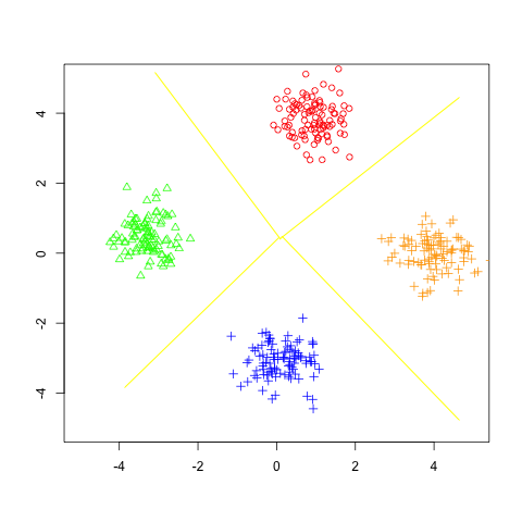
Figure 1: The clusters are separable by softmax$(Ax+b)$.

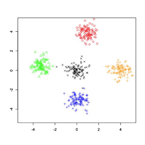
Figure 2: The central cluster cannot be separated by any softmax$(Ax+b)$.

IV Label Mapping

For a $N$-class classification problem, we define a Label Mapping (LM) as a sequence of map

$$f_{i}:\mathbb{Z}/N\mathbb{Z}\longrightarrow\mathbb{Z}/N_{i}\mathbb{Z},\quad i=1,2,...n,$$

where each $f_{i}$ is called a “site-position function”, and $n$ is called the “length” of the Label Mapping. If all the $N_{i}$ are equal to each other, we call it “simplex LM”; otherwise we call it “mixed LM”.

Generally, $N$ is a huge number, and $N_{i}$ are some numbers of middle size. We can reduce a $N$-classes classification problem to $n$’s classification problems of middle size through a LM. Suppose the training dataset is $\{x_{k},y_{k}\}$, where $x_{k}$ is feature and $y_{k}$ is label, there are two method to use DNN plus LM. The one is to use one network with $n$ outputs (Figure 4). The other one is to use $n$ networks, every network is trained as a base learner on the dataset $\{x_{k},f_{i}(y_{k})\}$ for $i=1,2,\cdots n$ (Figure 4). Considering the convenience of distributed training, we use method in Figure 4.

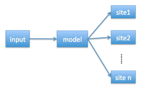
Figure 3: One network with n outputs

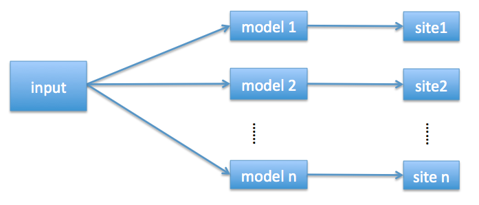
Figure 4: n networks with n outputs

A good LM should satisfy the follow properties:

Classes high separable. For two different labels $y,\tilde{y}$, there should be as many as possible site-position functions $f_{i}$ such that $f_{i}(y)\neq f_{i}(\tilde{y})$.

Base learners independence. When $y$ are selected randomly uniformly from $\mathbb{Z}/N\mathbb{Z}$, the mutual information of $f_{i}(y)$ and $f_{j}(y)$ approximate to 0 for $i\neq j$.

The property “classes high separable” ensures that for any two different classes, there are as many as possible base learners are trained to separate them. The property “base learners independence” ensures that the common part of the information learned by any two different base learners is as few as possible.

Remark. There are some similarities between LM and ECOC:

A ECOC of length $n$ for $N$ classes can be regarded as a sequence of maps

$$f_{i}:\mathbb{Z}/N\mathbb{Z}\longrightarrow\mathbb{Z}/2\mathbb{Z},\quad i=1,2,...n,$$

where each $f_{i}$ is called “bit-position function”.

We can see that comparing to ECOC, our LM does not need that the reduced classification problems are two-class classification problems. It even does not need that the reduced classification problems have the same number of classes.

In [42], two properties which a good error-correcting output binary code for a multi-class problem should be satisfied are proposed: ([42], section 2.3)

Row separation. Each codeword should be well-separated in Hamming distance from each of the other codewords.

Column separation. Each bit-position function should be uncorrelated with the functions to be learned for the other bit positions.

The property “Row separation” is similar to the property “Classes high separable” of LM, and the property “Column separation” is similar to the property ”Base learners independence”. ∎

We give 2 classes of LM, one is mixed LM, and the other is simplex LM, which satisfies the properties.

IV-A Mixed LM

We introduce the famous Prime Number Theorem ( [1], [35]) firstly:

Theorem 2.

(Prime Number Theorem) The density of prime number approximate $n$ is $1/\log n$.  $\blacksquare$

For the original label’s set $\mathbb{Z}/N\mathbb{Z}$, a small number k like 2, or 3, etc., and a small positive number $\epsilon\in(0,1)$, select $n$’s prime numbers $p_{1},p_{2},\cdots p_{n}$ in the domain $\left[N^{\frac{1}{k}},N^{\frac{1}{k-\epsilon}}\right)$. According to the Prime Number Theorem, there are about $\frac{k(N^{\frac{1}{k-\epsilon}}-N^{\frac{1}{k}})}{\log N}$ prime numbers in this domain.

We define a LM as

$$\begin{array}[]{ccc}\mathbb{Z}/N\mathbb{Z}&\longrightarrow&\prod_{i=1}^{n}\mathbb{Z}/p_{i}\mathbb{Z}\\ x&\mapsto&f_{i}(x)\end{array}$$

where $f_{i}(x)=x\mod p_{i}$. Then we have the following proposition:

Theorem 3.

For any $x\neq y\in\mathbb{Z}/N\mathbb{Z}$, there is at most $k-1$’s $i$ s.t $f_{i}(x)=f_{i}(y)$.

Proof. Suppose there exist $k$’s different $i$ such, that $f_{i}(x)=f_{i}(y)$, we can suppose that

$$f_{i}(x)=f_{i}(y)\quad\mbox{ for }i=1,2,\cdots k$$

Then we have $x\equiv y\mod p_{i}$ for all $i=1,2,\cdots,k$.

Because $\{p_{i}\}$ are prime numbers, we have $x\equiv y\mod\prod_{i=1}^{k}p_{i}$. But we know $x,y\in\{0,1,\cdots N-1\}$, which in $\{0,1,\cdots\prod_{i=1}^{k}p_{i}-1\}$, hence $x=y$. $\blacksquare$

This theorem tells us that the mixed LM satisfies the “Classes high separable” property. Following, we prove that it satisfies the property “Base learners independence”.

Theorem 4.

Let $x$ be uniformly randomly selected from $\mathbb{Z}/N\mathbb{Z}$, we have that for any $i\neq j$, the mutual Information of $f_{i}(x)$ and $f_{j}(x)$ approximate 0.

In order to prove this theorem, we give a lemma firstly.

Lemma 5.

Let $x$ be uniformly randomly selected from $\mathbb{Z}/N\mathbb{Z}$, $q$ is an positive integral number, $t:=\lceil\frac{N}{q}\rceil$. Then we have that the probability of $(x\mod q)$ at every point in $\mathbb{Z}/q\mathbb{Z}$ are $\frac{t}{N}$ or $\frac{t-1}{N}$.

Proof. Because the pre-image of every point in $\mathbb{Z}/q\mathbb{Z}$ under the map

$$\begin{array}[]{rcl}\mathbb{Z}/N\mathbb{Z}&\longrightarrow&\mathbb{Z}/q\mathbb{Z}\\ x&\mapsto&(x\mod q)\end{array}$$

is a set of $t$ or $t-1$ elements. ∎

Now, we proof the theorem 4:

Proof of Theorem 4: Let $t_{i}:=\lceil\frac{N}{p_{i}}\rceil$ and $s_{ij}=\lceil\frac{N}{p_{i}p_{j}}\rceil$ for every $i,j$. We have that the probabilities of $f_{i}(x)$ at every point in $\mathbb{Z}/p_{i}\mathbb{Z}$ are $\frac{t_{i}}{N}$ or $\frac{t_{i}-1}{N}$ and the probabilities of $(f_{i}(x),f_{j}(x))$ at every point in $\mathbb{Z}/p_{i}\mathbb{Z}\times\mathbb{Z}/p_{j}\mathbb{Z}\cong\mathbb{Z}/p_{i}p_{j}\mathbb{Z}$ are $\frac{s_{ij}}{N}$ or $\frac{s_{ij}-1}{N}$ by using the lemma 5.

We know that the mutual information of $y_{i}=f_{i}(x)$ and $y_{j}=f_{j}(x)$ is

$$I(Y_{i};Y_{j})=\sum_{(y_{i},y_{j})\in\mathbb{Z}/p\mathbb{Z}\times\mathbb{Z}/p\mathbb{Z}}p_{i,j}(y_{i},y_{j})\log\frac{p_{i,j}(y_{i},y_{j})}{p_{i}(y_{i})p_{j}(y_{j})}$$

a.) When $k=2$, we have $N<p_{i}p_{j}$ and hence $s=1$ and $p_{i,j}(y_{i},y_{j})=\frac{1}{N}$ on $N$’s point in $\mathbb{Z}/p\mathbb{Z}\times\mathbb{Z}/p\mathbb{Z}$ and $0$ on other points. Hence we have

$$\begin{array}[]{rl}I(Y_{i};Y_{j})&\leq\sum_{(y_{i},y_{j})\in\mathbb{Z}/p\mathbb{Z}\times\mathbb{Z}/p\mathbb{Z}}p_{i,j}(y_{i},y_{j})\log\frac{p_{i,j}(y_{i},y_{j})}{\frac{(t_{i}-1)(t_{j}-1)}{N^{2}}}\\ &=N\times\frac{1}{N}\log\frac{1/N}{\frac{(t_{i}-1)(t_{j}-1)}{N^{2}}}\\ &=\log N-\log(t_{i}-1)-\log(t_{j}-1)\\ &<\log N-\log(\frac{N}{p_{i}}-1)-\log(\frac{N}{p_{j}}-1)\\ &\leq\log N-2\log(\frac{N^{\frac{1}{2}}}{N^{2-\epsilon}}-1)\\ &=-2\log(\frac{1}{N^{2-\epsilon}}-N^{-\frac{1}{2}})\\ &\rightarrow 0\quad\mbox{ as }N\rightarrow\infty\end{array}$$

b.) When $k\geq 3$, we have $p_{i}p_{j}<N^{\frac{2}{k-\epsilon}}<N$, and

$$\begin{array}[]{rl}&I(Y_{i};Y_{j})\\ =&\sum_{(y_{i},y_{j})\in\mathbb{Z}/p_{i}\mathbb{Z}\times\mathbb{Z}/p_{j}\mathbb{Z}}p_{i,j}(y_{i},y_{j})\log p_{i,j}(y_{i},y_{j})\\ &-\sum_{(y_{i},y_{j})\in\mathbb{Z}/p_{i}\mathbb{Z}\times\mathbb{Z}/p_{j}\mathbb{Z}}p_{i,j}(y_{i},y_{j})(\log p_{i}(y_{i})+\log p_{j}(y_{j}))\\ =&\sum_{(y_{i},y_{j})\in\mathbb{Z}/p_{i}\mathbb{Z}\times\mathbb{Z}/p_{j}\mathbb{Z}}p_{i,j}(y_{i},y_{j})\log p_{i,j}(y_{i},y_{j})\\ &-\sum_{y_{i}\in\mathbb{Z}/p_{i}\mathbb{Z}}p_{i}(y_{i})\log p_{i}(y_{i})-\sum_{y_{j}\in\mathbb{Z}/p_{j}\mathbb{Z}}p_{j}(y_{j})\log p_{j}(y_{j})\\ \leq&p_{i}p_{j}\frac{s_{ij}}{N}\log(\frac{s_{ij}}{N})-p_{i}\frac{t_{i}-1}{N}\log\frac{t_{i}-1}{N}-p_{j}\frac{t_{j}-1}{N}\log\frac{t_{j}-1}{N}\end{array}$$

Because

$$\begin{array}[]{rcl}(s_{ij}-1)p_{i}p_{j}&<N\leq&s_{ij}p_{i}p_{j}\\ (t_{i}-1)p_{i}&<N\leq&t_{i}p_{i}\\ (t_{j}-1)p_{j}&<N\leq&t_{j}p_{j}\end{array}$$

We have

$$\begin{array}[]{rl}&I(Y_{i};Y_{j})\\ <&(1+\frac{p_{i}p_{j}}{N})\log(\frac{1}{p_{i}p_{j}}+\frac{1}{N})\\ &-(1-\frac{p_{i}}{N})\log(\frac{1}{p_{i}}-\frac{1}{N})-(1-\frac{p_{j}}{N})\log(\frac{1}{p_{j}}-\frac{1}{N})\\ =&\log\frac{\frac{1}{p_{i}p_{j}}+\frac{1}{N}}{(\frac{1}{p_{i}}-\frac{1}{N})(\frac{1}{p_{j}}-\frac{1}{N})}+\frac{p_{i}p_{j}}{N}\log(\frac{1}{p_{i}p_{j}}+\frac{1}{N})\\ &+\frac{p_{i}}{N}\log(\frac{1}{p_{i}}-\frac{1}{N})+\frac{p_{j}}{N}\log(\frac{1}{p_{j}}-\frac{1}{N})\\ \leq&\log(1+\frac{p_{i}p_{j}}{N})-\log(1-(\frac{1}{p_{i}}+\frac{1}{p_{j}})\frac{p_{i}p_{j}}{N}+\frac{1}{N^{2}})\\ \leq&\log(1+\frac{p_{i}p_{j}}{N})-\log(1-(\frac{1}{p_{i}}+\frac{1}{p_{j}})\frac{p_{i}p_{j}}{N})\\ =&O(\frac{p_{i}p_{j}}{N})+O((\frac{1}{p_{i}}+\frac{1}{p_{j}})\frac{p_{i}p_{j}}{N})\\ =&O(\frac{p_{i}p_{j}}{N})\\ =&O(N^{\frac{2}{k-\epsilon}-1})\\ =&O(N^{\frac{2+\epsilon-k}{k-\epsilon}})\rightarrow 0\quad\mbox{as}\quad N\rightarrow\infty\end{array}$$

$\blacksquare$

This theorem tells us that, the mixed LM satisfies the property “Base learners independence”.

IV-B Simplex LM

IV-B1 p-adic representation

For any prime number $p$, we can represent any non-negative integral number $x$ less than $p^{k}$ as the unique form $x=x_{0}+x_{1}p+\cdots+x_{k-1}p^{k-1}\quad(x_{i}\in\mathbb{Z}/p\mathbb{Z})$, which gives a bijection

$$\mathbb{Z}/p^{k}\mathbb{Z}\longrightarrow\mathbb{F}_{p}^{k}$$

For the classification problem of $N$-classes and any small positive integral number $k$ (for example, k=2, 3), let $\epsilon$ in (0,1) be a small positive real number, and take the a prime number $p$ in the domain $[N^{\frac{1}{k}},N^{\frac{1}{k-\epsilon}}]$. (By The Prime Number Theorem [35][1], the number of prime number in the domain $[N^{\frac{1}{k}},N^{\frac{1}{k-\epsilon}}]$ is about $k(N^{\frac{1}{k-\epsilon}}-N^{\frac{1}{k}})/\log N$ ), and get a injection

$$\mathbb{Z}/N\mathbb{Z}\longrightarrow\mathbb{Z}/p^{k}\mathbb{Z}\longrightarrow\mathbb{F}_{p}^{k}$$

by p-adic representation. Then we can combine this map with any injection $\mathbb{F}_{p}^{k}\longrightarrow\mathbb{F}_{p}^{n}$ to get $p$-ary simplex LM.

IV-B2 Singleton bound and MDS code

In coding theory, the Singleton bound, named after Richard Colome Singleton [4], is a relatively crude upper bound on the size of an arbitrary q-ary code $C$ with block length $n$, size $M$ and minimum distance $d$.

The minimum distance of a set C of codewords of length $n$ is defined as

$$d=\min_{\{x,y\in C:x\neq y\}}d(x,y)$$

where $d(x,y)$ is the Hamming distance between $x$ and $y$. The expression $A_{q}(n,d)$ represents the maximum number of possible codewords in a q-ary block code of length $n$ and minimum distance $d$. Then the Singleton bound states that

Theorem 6.

(Richard Collom Singleton) $A_{q}(n,d)\leq q^{n-d+1}$.  $\blacksquare$

The code achieving Singleton bound is called MDS (maximal distinct separate) code.

It is easy to see that, for a fixed original ID’s number $N$, code length $n$, MDS codes are the codes which most satisfies the property “Class high separable”. Fortunately, for big prime number or power over prime number $q$, there are some nontrivial MDS codes found, for example the Reed-Solomon code[25].

Theorem 7.

(Reed and Solomon) For $n$’s different elements $x_{1},x_{2},\cdots,x_{n}$ in $\mathbb{F}_{q}$, the code defined by the composite of the map

$$\begin{array}[]{rcl}\mathbb{F}^{k}_{q}&\longrightarrow&\mathbb{F}_{q}[x]_{deg<k}\\ (a_{0},\cdots,a_{k-1})&\mapsto&a_{0}+a_{1}x+\cdots a_{k-1}x^{k-1}\end{array}$$

and the map

$$\begin{array}[]{rcl}\mathbb{F}_{q}[x]_{deg<k}&\longrightarrow&\mathbb{F}_{q}^{n}\\ f(x)&\mapsto&(f(x_{1}),\cdots f(x_{n}))\end{array}$$

is a MDS code.  $\blacksquare$

In this paper, we use only the Reed-Solomon code with q=p be a prime number.

Remark. In the case of ECOC, the property similar to “Class high separable” is ”Row separation”. If there exists a nontrivial binary MDS code, it will be the code most satisfies “Row separation” also. But unfortunately, it has not find any nontrivial binary MDS code yet up to now. In fact, for some situation, the fact that there are not any nontrivial binary MDS code is proved. ([36] and Proposition 9.2 on p. 212 in [10] ). This is an advantage of simplex LM better than ECOC also.

IV-B3 Separability and independency

We can combine the $p$-adic representation map with a Reed-Solomon encoder over field $\mathbb{F}_{p}$ to get a simplex LM for any prime number $p$. The above theorem ensures that, this code satisfies the property “Classes high separable”. We will prove that, it satisfies the property “Base learners independence” also.

Theorem 8.

If $u$ is a random variable with uniform distribution on $\mathbb{Z}/N\mathbb{Z}$, $y_{i}$ and $y_{j}$ are the i-site value and j-site value ($i\neq j$) of the codeword of $u$ under the simplex LM described above, then the mutual information of $y_{i}$ and $y_{j}$ approach to $0$ when $N$ grows up.

The proof of this theorem is similar to the proof of the theorem 4, we omit it due to space limitations.

$\blacksquare$

IV-C Decode Algorithm

Suppose we used the LM

$$f_{i}:\mathbb{Z}/N\mathbb{Z}\longrightarrow\mathbb{Z}/N_{i}\mathbb{Z},\quad i=1,2,...n,$$

to reduce a classification problem of class number $N$ to the classification problems of class number $N_{i}$’s, and trained $n$ base learner for every $f_{i}$, the output of every base learner $i$ is a distribution $P_{i}$ on $\mathbb{Z}/N_{i}\mathbb{Z}$. Now, for a input feature data, how we collect the output $\{P_{i}:i=1,2,\cdots,n\}$ of every base learner to get the predict label?

In this paper, we search the $a\in\mathbb{Z}/N\mathbb{Z}$ such that $\sum_{i}\log P_{i}(f_{i}(a))$ is maximal, and let such $a$ be the decoded label.

In fact, $\sum_{i}\log P_{i}(f_{i}(a))=-\sum_{i}KL(f_{i\star}\delta(x-a)||P_{i})$ , where $\delta(x-a)$ is the Delta distribution at $a\in\mathbb{Z}/N\mathbb{Z}$, and $f_{i\star}\delta(x-a)$ is the marginal distribution of $\delta(x-a)$ induced by $f_{i}$. This decode algorithm is that find the Delta distribution on $\mathbb{Z}/N\mathbb{Z}$ such that the marginal distribution on every $\mathbb{Z}/N_{i}\mathbb{Z}$ included from it is as closed to $P_{i}$ as possiple.

V Numeric experiments

We give performance of LM on three dataset, namely, the dataset Cifar-100 [44] , the dataset CJK characters and the dataset Republic. The CIFAR-100 dataset consists of 60000 32x32 color images in 100 classes, with 500 training images and 100 testing images per class. The dataset CJK characters is the grey-level image of size 139x139 of 20901 CJK characters (0x4e00 $\sim$ 0x9fa5) in 8 fonts. The dataset Republic is a text with 118684 words and 7409 unique words in the vocabulary.

We use a simple CNN network, which dimension in the last but one layer is 128, with a one-hot encoding as the baseline for the cifar-100 dataset.

We use an inception V3 network [43], which dimension in the last but one layer is 2048, with a one-hot encoding as the baseline for the CJK characters dataset.

We use a RNN network which dimension in the last but one layer is 100, with a one-hot encoding as the baseline for the dataset “Republic”.

We will see that the accuracy of LM increases with the increasing of its length on all the datasets. But the accuracy of LM on (cifar-100, simple CNN) is difficult to be higher than the one-hot, the accuracy of LM on (CJK character, inception V3) better than one-hot with the almost same number of parameters, and the accuracy of LM on (Republic, RNN) is much better than one-hot with more number of parameters.

Why there is a such big difference of accuracy in three situations? Because the dimension of the last but one layer of the simple CNN is bigger than the class number of cifar-100 dataset, and hence the one-hot encoding can brought into full play the power of simple CNN. But the dimension of the last but one layer of inception V3 is less than the class number of dataset CJK character, which causes that the one-hot encoding can not bring the power of inception V3 into full play. Moreover, the dimension of the last but one layer of RNN is much less than the class number of dataset Republic, which causes that the one-hot encoding absolutely can not bring the power of RNN into full play (According to the relation of the dimension of the last but one layer and the class number discussed in section III.)

V-A On a dataset of small class number

We use a simple CNN network on the dataset Cifar-100. The simple CNN network includes 3 convolution layers and a full-connected layer. The sizes of convolution kernels are $3\times 3$, and the weigth of the three convolution layers are 32, 64, 128 respectively. After each convolution layer, a $2\times 2$ average poling layer is applied. After the 3rd pooling layer and the full-connection layer, we use dropout layer of probability 0.25. The network structure is like in Figure 6.

Note the dimension 128 of the last but one layer is greater than the class number 100, hence the one-hot encoding can bring the power of simple CNN into full play. In this experiment the LM is difficult to surpass the one-hot, but we can see the accuracy increases with the increasing of length of LM. We will see the accuracy of LM is greater than the accuracy of ECOC also.

V-A1 The performance of simplex LM of different length

We use the simplex LM defined above with $p=11,k=2$ and $n=3,4,5,6$. The simplex LM can be writn as

$$f_{i}:\mathbb{Z}/N\mathbb{Z}\longrightarrow\mathbb{Z}/N_{i}\mathbb{Z},\quad i=1,2,\cdots n$$

where $N=100$, and $f_{i}(x)=((x\mod p)+floor(x/p)i)\mod p$.

We train the networks with batch size=128 and 390 batch per epoch. The Figure 6 shows the accuracy of these simplex LMs with the single CNN on dataset cifar-100:

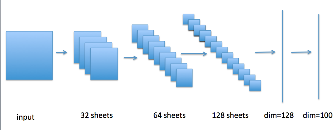
Figure 5: The network structure of simple CNN

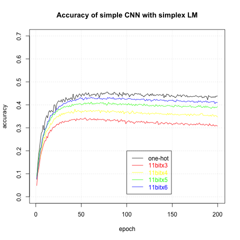
Figure 6: The accuracy of simplex LMs of n=3,4,5,6 and one-hot

In Figure 6, the horizontal axis is the traning epoch, and the vertical axis is the validation accuracy. The five curves, which colors are red, yellow, green, blue and black respectively, are the epoch-accuracy curves of the simple CNN with simplex LM defined above with $p=11,k=2$ and $n=3,4,5,6$ and the one-hot encoding respectively.

We can see, the accuracy of these networks with simplex LM and one-hot encoding increase in the first 50$\sim$80 epoch, and then a little of overfitting occur. The accuracy of simple CNN with simplex LM increases with the increasing of length of the LM, it approximates the accuracy of one-hot as $n$ increase, but it is difficult to surpass the one-hot. The reason is that the dimension of the last but one layer of the simple CNN is bigger than the class number of cifar-100 dataset, and hence the one-hot encoding can bring the power of simple CNN into full play.

V-A2 The performance of mixed LM of different length

We use the mixed LMs defined above with $k=2$ and $\{p_{i}\}\subset\{11,13,17,19,23\}$. The mixed LM can be writen as

$$f_{i}:\mathbb{Z}/N\mathbb{Z}\longrightarrow\mathbb{Z}/p_{i}\mathbb{Z},\quad i=1,2,\cdots n$$

where $N=100$, and $f_{i}(x)=x\mod p_{i}$.

The Figure 8 shows the accuracy of these mixed LMs with the simple CNN on dataset cifar-100:

In Figure 8, the horizontal axis is the traning epoch, and the vertical axis is the validation accuracy. The five curves, which colors are red, yellow, green, blue and black respectively, are the epoch-accuracy curves of the simple CNN with simplex LM defined above with $\{p_{i}\}$ are $\{11,13\}$, $\{11,13,17\}$, $\{11,13,17,19\}$, $\{11,13,17,19,23\}$ and the one-hot encoding respectively.

We can see, the accuracy of these networks with mixed LM and one-hot encoding increase in the first 50$\sim$80 epoch, and then a little of overfitting occur. The accuracy of simple CNN with mixed LM increases with the increasing of length of the LM, it approximates the accuracy of one-hot as $n$ increase, but it is difficult to surpass the one-hot. The reason is that the dimension of the last but one layer of the simple CNN is bigger than the class number of cifar-100 dataset, and hence the one-hot encoding can brought into full play the power of simple CNN.

V-A3 Compare LM with ECOC

On this subsection, we compare the performance of LM and ECOC. We show the accuracy of the following LMs (ECOC is a special case of LM) with the simple CNN network on the dataset cifar-100:

a. A ECOC of n=7

b. A simplex LM of p=11 and n=3.

c. A mixed LM of $\{p_{i}\}=\{11,13,17\}$.

For the ECOC of $n=7$, we encode a label $y\in\{0,1,\cdots,99\}$ to its binary representation of length 7.

The simplex LM can be written as

$$f_{i}:\mathbb{Z}/N\mathbb{Z}\longrightarrow\mathbb{Z}/N_{i}\mathbb{Z},\quad i=1,2,\cdots n$$

where $N=100$, and $f_{i}(x)=((x\mod p)+floor(x/p)i)\mod p$.

The mixed LM can be writn as

$$f_{i}:\mathbb{Z}/N\mathbb{Z}\longrightarrow\mathbb{Z}/p_{i}\mathbb{Z},\quad i=1,2,\cdots n$$

where $N=100$, and $f_{i}(x)=x\mod p_{i}$.

The number of parameters of the three method are 1112622, 480321, 481353. The accuracies of the three method is like in Figure 8. We can see, the accuracies of LMs are better than the ECOC even when the number of parameters of LM is much less than one of ECOC.

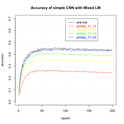
Figure 7: The accuracy of mixed LMs of n=2,3,4,5 and one-hot

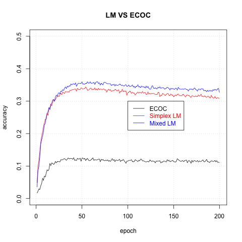
Figure 8: Compare LMs with ECOC

V-B On a dataset “CJK Characters” of big class number

We use the Inception V3 network and LM on the dataset “CJK characters”. CJK is a collective term for the Chinese, Japanese, and Korean languages, all of which use Chinese characters and derivatives (collectively, CJK characters) in their writing systems. The data set “CJK characters” is the grey-level image of size 139x139 of 20901 CJK characters (0x4e00 $\sim$ 0x9fa5) in 8 fonts , these fonts are in the paths in Figure 9 of a MacBook Pro with OS X version 10.11.

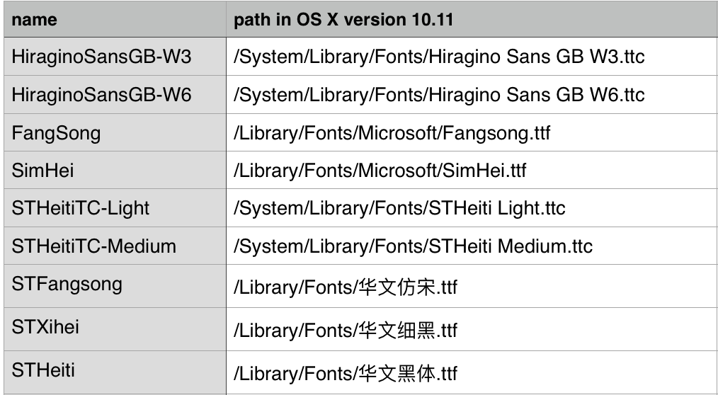
Figure 9: The fonts and their paths of fonts in OS X version 10.11

We use 7 fonts as the train set, and other one font as the test set. We use inception v3 network as base learner, and train the networks using batch size=128 and 100 batch per an epoch.

Noted the dimension 2048 of the last but one layer of Inception V3 is much less than the class number 20901, hence the one-hot encoding can not bring the power of simple CNN into full play. In this experiment we can see the accuracy increases with the increasing of length of LM, and the LM is easy to surpass the one-hot. We will see the accuracy of LM is greater than the accuracy of ECOC also.

This section is divided into 3 parts. The part 1, 2 shows the performance of simplex LM and mixed LM respectively. Their accuracies increase with the increasing of length, and surpass the one-hot when length is greater or equal to 3. The part 3 compares the performance of LMs with the ECOC.

V-B1 The performance of simplex LM of different length

In this part, we shows how the accuracy of simplex LM increases with the increasing of length of LM. We also show that when the length increases, the performance of LM is better than the network with one-hot encoding.

We use the simplex LM with $p=181$ and $k=2$. The simplex LM can be writn as

$$f_{i}:\mathbb{Z}/N\mathbb{Z}\longrightarrow\mathbb{Z}/N_{i}\mathbb{Z},\quad i=1,2,\cdots n$$

where $N=21901$, and $f_{i}(x)=((x\mod p)+floor(x/p)i)\mod p$. The accuracies of theses simplex LMs are like in Table I.

In the table I, the accuracies in epoch 20, 40, 60, 80 are showed. The column “epoch” means the epoch number in training, the column “n sites” is the accuracy of the inception V3 networks with simplex LM of n sites for $n=2,3,\cdots 6$, and the column “one-hot” is the accuracy of the inception V3 with one-hot encoding.

We see that, the accuracies of LM of all the site numbers increase with the increasing of training epoch. The accuracy of LM increase with the increasing of sites number also. When the sites number is equal to 3, the parameters number of LM is approximate to the parameters number of one-hot, but the accuracy of LM is greater than the one-hot with softmax or negative sampling.

Remark. In the one-hot network in the table I, the last layer has dimension 20901, but the last but one layer has dimension only 2048. If we set the dimension of the last but one layer to 20900, the performance may be better, but our GPU does not have such huge memory.

Remark. In the term “one-hot with negative sampling” in the table I, the using negative sampling ratio is 10:1.

ep.	2 sites	3 sites	4 sites	5 sites	6 sites	one-hot	one-hot with
						with	negative
						softmax	sampling
20	0.0118	0.0318	0.0604	0.0585	0.0640	0.0325	0.0004
40	0.6657	0.9373	0.9812	0.9865	0.9878	0.5152	0.0007
60	0.8172	0.9840	0.9943	0.9964	0.9968	0.9399	0.0019
80	0.8684	0.9920	0.9978	0.9984	0.9988	0.9854	0.0031
param. num.	$2.21$	$2.21$	$2.21$	$2.21$	$2.21$	6.46	6.46
($10^{7}$)	$\times 2$	$\times 3$	$\times 4$	$\times 5$	$\times 6$

TABLE I: Performance of Simplex Label Mappings

V-B2 The performance of mixed LM of different length

In this part, we show how the accuracy of mixed LM increases with the increasing of length of LM. We also show that when the length increases, the performance of LM is better than the network with one-hot encoding.

We use the mixed Label Mappings with primes in {149, 151, 157, 163, 167, 173, 179}. The mixed LM can writn as

$$f_{i}:\mathbb{Z}/N\mathbb{Z}\longrightarrow\mathbb{Z}/N_{i}\mathbb{Z},\quad i=1,2,\cdots n$$

where $N=21901$, and $f_{i}(x)=x\mod p_{i}$, $p_{1}=149,p_{2}=151,\cdots$.

The accuracies are like in following table II. In this table, the accuracies in epoch 20, 40, 60, 80 are showed. The column “epoch” means the epoch number in training, the column “n sites” is the accuracy of the inception V3 networks with simplex LM of n sites for $n=2,3,\cdots 7$, and the column “one-hot” is the accuracy of the inception V3 with one-hot encoding.

We see that, the accuracies of mixed LM of all the site numbers increase with the increasing of training epoch. The accuracy of mixed LM increases with the increasing of sites number also. When the sites number is equal to 3, the parameters number of LM is approximate to the parameters number of one-hot, but the accuracy of LM is greater than the one-hot.

Remark. In the one-hot network in the table II, the last layer has dimension 20901, but the last but one layer has dimension only 2048. If we set the dimension of the last but one layer to 20900, the performance may be better, but our GPU does not have such huge memory.

Remark. In the term “one-hot with negative sampling” in the table II, the using negative sampling ratio is 10:1.

ep.	2 sites	3 sites	4 sites	5 sites	6 sites	7 sites	one-hot with	one-hot with
							softmax	negative sampling
20	0.0081	0.0101	0.0100	0.0309	0.0585	0.0926	0.0325	0.0004
40	0.6130	0.8100	0.8707	0.9656	0.9851	0.9903	0.5152	0.0007
60	0.7629	0.9765	0.9925	0.9957	0.9967	0.9974	0.9399	0.0019
80	0.8757	0.9912	0.9971	0.9980	0.9982	0.9987	0.9854	0.0031
param. num.	$2.21$	$2.21$	$2.21$	$2.21$	$2.21$	$2.21$	6.46	6.46
($10^{7}$)	$\times 2$	$\times 3$	$\times 4$	$\times 5$	$\times 6$	$\times 7$

TABLE II: Performance of Mixed Label Mappings

V-B3 Compare LM with ECOC

We show the arccuracies of the following ensemble methods with the inception V3 network on the CJK dataset:

a. A 15 bits ECOC corresponding to the binary representation of label $0\sim 20900$

b. A 2 sites simplex LM of p=181 and n=2

c. A 2 sites mixed LM of p in {149, 151}

The three settings are the minimal setting for the three methods respectively, it means, if we reduce any bit of the encoding or any site of the label mapping, the encoding or the label mapping will be not injection. The accuracies are in Table III:

ep.	ECOC of 15 bit	simplex LM of 2 sites	mixed LM of 2 sites
20	0.0069	0.0118	0.0081
40	0.0795	0.6657	0.6130
60	0.3660	0.8172	0.7629
80	0.5740	0.8684	0.8757
param. num. ($10^{7}$)	$2.18\times 15$	$2.21\times 2$	$2.21\times 2$

TABLE III: Comparing of ECOC and Label Mappings

We can see, even when the base learner number 2 of LM is much less than the base learner number 15 of ECOC, and the parameters number of LM is much less than the parameters number of ECOC, the performance of LM is better than the ECOC.

V-C On the dataset “Republic”

The Republic ([45],[46]) is a Socratic dialogue, written by Plato around 380 BC, concerning justice, the order and character of the just, city-state, and the just man.

We use the following produce firstly:

a). Replace ‘-’ with a white space.

b). Split words based on white space.

c). Remove all punctuation from words.

d). Remove all words that are not alphabetic to remove standalone punctuation tokens.

e). Normalize all words to lowercase.

After the produce, there are 118684 words in the produced text, and 7409 unique words in the vocabulary.

We construct a network which use the 50 previous words as input and predict the current word. Because both the input and output are categorical with big number of classes, we use the LM method not only for output, but for input also.

In fact, for a LM

$$f:\mathbb{Z}/N\mathbb{Z}\longrightarrow\prod_{i=1}^{n}\mathbb{Z}/N_{i}\mathbb{Z}$$

We get a sparse encode method

$$f:\mathbb{Z}/N\mathbb{Z}\longrightarrow\prod_{i=1}^{n}\mathbb{Z}/N_{i}\mathbb{Z}\longrightarrow\prod_{i=1}^{n}\mathbb{F}_{2}^{N_{i}}\cong\mathbb{F}_{2}^{\sum N_{i}}$$

induced by this LM naturally. The middle map is defined by $(x_{i})_{i}\mapsto\mbox{ (The one-hot encoding of }x_{i}\mbox{ of length }N_{i})_{i}$. Use this map, we can get a $n$-hot code of length $\sum_{i}N_{i}$ for every label in $\mathbb{Z}/N\mathbb{Z}$, which can be used as input encoding.

The network include an input encoding layer of dimension $\sum_{i}N_{i}$ , an embedding layer of dimension 150, two LSTM layer of dimension 100, a dense layer of dimension 100, and a dense output layer. After every output layers of dimension $N_{i}$, a softmax is used. The structure of the network is like in Figure 10. In Figure 10 we draw only one encoding unit and one embedding unit, in fact there are encoding unit and embedding unit before every LSTM cell in first LSTM layer, but the weight of the encoding units and embedding units are same respectively.

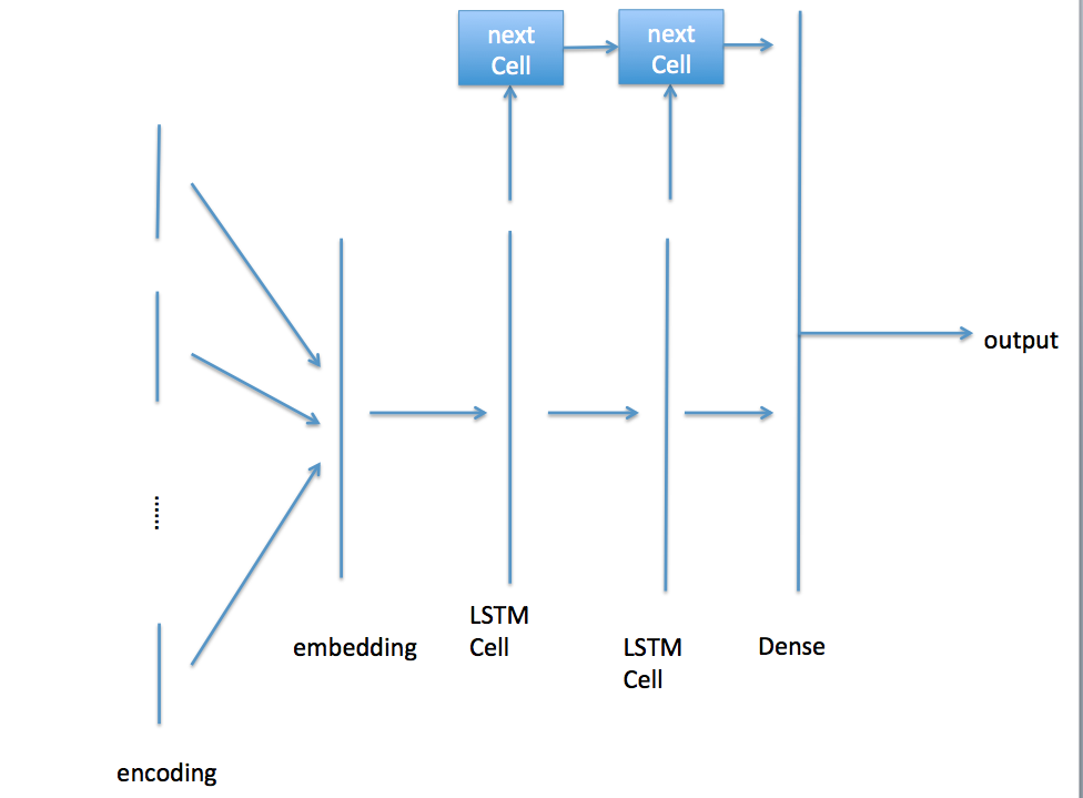
Figure 10: The network structure

The performance is like following table IV, where the mixed LM of 2 sites use $\{N_{i}\}=\{107,109\}$, the mixed LM of 4 sites use $\{N_{i}\}=\{107,109,113,127\}$, the mixed LM of 6 sites use $\{N_{i}\}=\{107,109,113,127,131,137\}$. The simplex LM use the prime number $127$.

input	output	par. num.	2	4	6	8	10
one-hot	one-hot	2.9E6	0.0946	0.1265	0.1379	0.1471	0.1540
	softmax
one-hot	one-hot	2.9E6	0.048	0.058	0.058	0.058	0.058
	negative sampling
724 bit cut-off	724 bit cut-off	3.7E5	0.0589	0.1076	0.1245	0.1272	0.1321
mix. LM of 6 sites	mix. LM of 2 sites	6.2E5	0.1331	0.1402	0.1366	0.1358	0.1189
mix. LM of 6 sites	mix. LM of 4 sites	1.2E6	0.1609	0.1722	0.1795	0.1836	0.1845
mix. LM of 6 sites	mix. LM of 6 sites	1.9E6	0.1590	0.1731	0.1812	0.1849	0.1865
sim. LM of 6 sites	sim. LM of 2 sites	6.3E5	0.1453	0.1505	0.1531	0.1522	0.1444
sim. LM of 6 sites	sim. LM of 4 sites	1.3E6	0.1586	0.1685	0.1759	0.1805	0.1832
sim. LM of 6 sites	sim. LM of 6 sites	1.9E6	0.1575	0.1694	0.1776	0.1814	0.1851

TABLE IV: Label Mapping for dataset “Republic”

We see that, the accuracies of LMs of all the site numbers increase with the increasing of training epoch basically. An overfitting occurs at epoch 10 when we use LM of 6 sites as input encoding and LM of 2 sites as output encoding, but it disappear with the increasing of number of sites of output encoding. The accuracies of LMs increase with the increasing of sites number. Even when the number of parameters used in LM is much less than the one-hot with softmax or one-hot with negative sampling, the performance of LM is better than one-hot.

There is an usually used method for big vocabulary in language model, i.e. the cut-off method: the most frequent words are encoded on-hot, and all other words are common encoded as ’$000\cdots 0001$’. If we view the LM of 6 sites with $\{N_{i}\}=\{107,109,113,127,131,137\}$ as a binary encoding, its length is 107+109+113+127+131+137=724. We see that, the performance of cut-off method of 724 bits is much lower than the mixed LM of 6 sites with $\{N_{i}\}=\{107,109,113,127,131,137\}$.

VI Conclusion

We give an ensemble method so called Label Mapping (LM), which translates a classification problem of huge class number to several classification sub-problems of middle class number, and trains a base learner for every sub-problem. The necessary number of base learners is sub-linear grow with the growing of class number.

We propose two design principles, namely, Classes high separable and Base learners independence of Label Mapping, and give two classes of Label Mapping and prove they are satisfying the two principles.

As numeric experiments, we show the accuracies of LM on three datasets, namely, the dataset Cifar-100, the dataset CJK characters and the dataset “Republic”. On all the datasets, the accuracies of LM increase with the increasing of length. When the class number is big (the dataset CJK characters and the dataset “Republic”), specially, the class number is much greater than the dimension of the last but one layer of the network, the accuracy of LM plus Network is better than the one-hot encoding plus Network with almost same or big number of parameters. We compare LM with the classical method ECOC also, the accuracy of LM is much greater than the accuracy of ECOC of bigger number of parameters.

References

- [1] Bernhard Riemann. Ueber die Anzahl der Primzahlen unter einer gegebenen Grosse. Monatsberichte der Berliner Akademie, November 1859.
- [2] https://en.wikipedia.org/wiki/Prime_number_theorem.
- [3] Irving S. Reed and Gustav Solomon. Polynomial codes over certain finite fields. J. SIAM, 8:300-304, 1960.
- [4] Richard C. Singleton. Maximum distance q-nary codes. IEEE Transactions on Information Theory, 10(2):116–118, April 1964.
- [5] Morin, F., Bengio, Y. (2005). Hierarchical Probabilistic Neural Network Language Model.
- [6] Tomas Mikolov, Ilya Sutskever, Kai Chen, Greg S Corrado, and Jeff Dean. 2013. Distributed representations of words and phrases and their compositionality. In Advances in NIPS, pages 3111–3119.
- [7] E. L. Allwein, R. E. Schapire, and Y. Singer. Reducing multiclass to binary: A unifying approach for margin classifiers. The Journal of Machine Learning Research. Volume 1, 2001, pages 113-141.
- [8] Sejnowski T.J., Rosenberg C.R.(1987).Parallel networks that learn to pronounce english text. Journal of Complex Systems,1(1), 145-168.
- [9] Shu Lin; Daniel Costello (2005). Error Control Coding (2 ed.). Pearson. ISBN 0-13-017973-6. Chapter 4.
- [10] L. R. Vermani. Elements of Algebraic Coding Theory. CRC Press, 1996.
- [11] E. Guerrini and M. Sala. A classification of MDS binary systematic codes. BCRI preprint, www.bcri.ucc.ie 56, UCC, Cork, Ireland, 2006.
- [12] T. G. Dietterich and G. Bakiri. Solving multiclass learning problems via error-correcting output codes. Journal of artificial intelligence research, pp. 263–286, 1995.
- [13] E. L. Allwein, R. E. Schapire, and Y. Singer. Reducing multiclass to binary: A unifying approach for margin classifiers. The Journal of Machine Learning Research, 1:113–141, 2001.
- [14] A. Passerini, M. Pontil, and P. Frasconi. New results on error correcting output codes of kernel machines. Neural Networks, IEEE Transactions on, 15(1):45–54, 2004.
- [15] Langford, J., and Beygelzimer, A. 2005. Sensitive error correcting output codes. In COLT.
- [16] G. Hinton and R. Salakhutdinov. Reducing the dimensionality of data with neural networks. Science, 313(5786):504–507, 2006
- [17] S. Escalera, O. Pujol, and P. Radeva. Ecoc-one: A novel coding and decoding strategy. In ICPR, volume 3, pp. 578–581, 2006.
- [18] O. Pujol, P. Radeva, and J. Vitria. Discriminant ECOC: a heuristic method for application dependent design of error correcting output codes. Pattern Analysis and Machine Intelligence, IEEE Transactions on, 28(6):1007–1012, 2006.
- [19] O. Pujol, S. Escalera, and P. Radeva. An incremental node embedding technique for error correcting output codes. Pattern Recognition, 41(2):713–725, 2008.
- [20] S. Escalera, O. Pujol, and P. Radeva. Separability of ternary codes for sparse designs of errorcorrecting output codes. Pattern Recognition Letters, 30(3):285–297, 2009.
- [21] G. Zhong, K. Huang, and C.-L. Liu. Joint learning of error-correcting output codes and dichotomizers from data. Neural Computing and Applications, 21(4):715–724, 2012.
- [22] G. Zhong and M. Cheriet. Adaptive error-correcting output codes. In IJCAI, 2013.
- [23] G. Zhong and C.-L. Liu. Error-correcting output codes based ensemble feature extraction. Pattern Recognition, 46(4):1091–1100, 2013.
- [24] Yang, Luo, Loy, Shum, Tang. Deep Representation Learning with Target Coding. Twenty-Ninth AAAI Conference on Artificial Intelligence, 2015 :3848-3854.
- [25] Irving S. Reed and Gustav Solomon. Polynomial codes over certain finite fields. JSIAM volume 8, number 2, jun 1960, pages 300-304.
- [26] S. Escalera, O. Pujol, and P. Radeva. Ecoc-one: A novel coding and decoding strategy. International Conference on Pattern Recognition. Volume 3, 2006, pages 578-581.
- [27] O. Pujol, P. Radeva, and J. Vitria. Discriminant ECOC: a heuristic method for application dependent design of error correcting output codes. IEEE Transactions on Pattern Analysis and Machine Intelligence. Volume 28, number 6, 2006, pages 1007-1012.
- [28] O. Pujol, S. Escalera, and P. Radeva. An incremental node embedding technique for error correcting output codes. Pattern Recognition. Volume 41, number 2, 2008, pages 713-725.
- [29] S. Escalera, O. Pujol, and P. Radeva. Separability of ternary codes for sparse designs of error-correcting output codes. Pattern Recognition Letters. Volume 30, number 3 2009, pages 285-297.
- [30] A. Passerini, M. Pontil and P. Frasconi. New results on error correcting output codes of kernel machines. IEEE Transactions on Neural Networks. Volume 15, number 1, 2004, pages 45-54.
- [31] Langford J., and Beygelzimer A. Sensitive error correcting output codes. International Conference on Computational Learning Theory. Volume 2459, number 3, 2005, pages 158-172.
- [32] Ghani R.. Using Error-Correcting Codes for Efficient Text Classification with a Large Number of Categories. KDD Lab Project Proposal. 2001.
- [33] Yang, Luo, Loy, Shum, Tang. Deep Representation Learning with Target Coding. Twenty-Ninth AAAI Conference on Artificial Intelligence. 2015, pages 3848-3854.
- [34] Jie Qin, Li Liu, Ling Shao, Fumin Shen, Bingbing Ni, Jiaxin Chen, Yunhong Wang. Zero-Shot Action Recognition With Error-Correcting Output Codes. The IEEE Conference on Computer Vision and Pattern Recognition (CVPR). 2017, pages 2833-2842.
- [35] Apostol T. M. Introduction to Analytic Number Theory. Springer-Verlag , 1976, New York.
- [36] E. Guerrini and M. Sala. A classification of MDS binary systematic codes. BCR preprint, 2006. www.bcri.ucc.ie/FILES/PUBS/BCRI_57.pdf
- [37] Niloufar Eghbali and Gholam AliMontazer. Improving multiclass classification using neighborhood search in error correcting output codes. Pattern Recognition Letters. Dec 2017, volume 100, number 1, pages 74-82.
- [38] Fa Zheng, Hui Xue, Xiaohong Chen, Yunyun Wang. Maximum Margin Tree Error Correcting Output Codes. Pacific Rim International Conference on Artificial Intelligence. 2016, pages 681-691.
- [39] Berger, A.: Error-Correcting Output Coding for text classification. In: IJCAI(1999)
- [40] Ghani, R.: Using error-correcting codes for text classification. Proceedings of ICML-00, 17th International Conference on Machine Learning (pp. 303–310). Stanford, US: Morgan Kaufmann Publishers, San Francisco, US.
- [41] Ghani, R. Using Error-Correcting Codes for Efficient Text Classification with a Large Number of Categories. KDD Lab Project Proposal.
- [42] T. G. Dietterich and G. Bakiri. Solving multiclass learning problems via error-correcting output codes. Journal of artificial intelligence research, 1995, p263-286.
- [43] Christian Szegedy, Vincent Vanhoucke, Sergey Ioffe, Jonathon Shlens, Zbigniew Wojna. Rethinking the Inception Architecture for Computer Vision. 2015. https://arxiv.org/abs/1512.00567
- [44] Alex Krizhevsky. Learning Multiple Layers of Features from Tiny Images. 2009. https://www.cs.toronto.edu/ kriz/cifar.html
- [45] https://en.wikipedia.org/wiki/Republic_(Plato)
- [46] http://www.gutenberg.org/cache/epub/1497/pg1497.txt