Deep Neural Networks with Multi-Branch Architectures Are
Less Non-Convex

Abstract

Several recently proposed architectures of neural networks such as ResNeXt, Inception, Xception, SqueezeNet and Wide ResNet are based on the designing idea of having multiple branches and have demonstrated improved performance in many applications. We show that one cause for such success is due to the fact that the multi-branch architecture is less non-convex in terms of duality gap. The duality gap measures the degree of intrinsic non-convexity of an optimization problem: smaller gap in relative value implies lower degree of intrinsic non-convexity. The challenge is to quantitatively measure the duality gap of highly non-convex problems such as deep neural networks. In this work, we provide strong guarantees of this quantity for two classes of network architectures. For the neural networks with arbitrary activation functions, multi-branch architecture and a variant of hinge loss, we show that the duality gap of both population and empirical risks shrinks to zero as the number of branches increases. This result sheds light on better understanding the power of over-parametrization where increasing the network width tends to make the loss surface less non-convex. For the neural networks with linear activation function and $\ell_{2}$ loss, we show that the duality gap of empirical risk is zero. Our two results work for arbitrary depths and adversarial data, while the analytical techniques might be of independent interest to non-convex optimization more broadly. Experiments on both synthetic and real-world datasets validate our results.

1 Introduction

Deep neural networks are a central object of study in machine learning, computer vision, and many other domains. They have substantially improved over conventional learning algorithms in many areas, including speech recognition, object detection, and natural language processing [28]. The focus of this work is to investigate the duality gap of deep neural networks. The duality gap is the discrepancy between the optimal values of primal and dual problems. While it has been well understood for convex optimization, little is known for non-convex problems. A smaller duality gap in relative value typically implies that the problem itself is less non-convex, and thus is easier to optimize. Our results establish that: Deep neural networks with multi-branch architecture have small duality gap in relative value.

Our study is motivated by the computational difficulties of deep neural networks due to its non-convex nature. While many works have witnessed the power of local search algorithms for deep neural networks [16], these algorithms typically converge to a suboptimal solution in the worst cases according to various empirical observations [52, 28]. It is reported that for a single-hidden-layer neural network, when the number of hidden units is small, stochastic gradient descent may get easily stuck at the poor local minima [27, 49]. Furthermore, there is significant evidence indicating that when the networks are deep enough, bad saddle points do exist [1] and might be hard to escape [15, 21, 10, 1].

Given the computational obstacles, several efforts have been devoted to designing new architectures to alleviate the above issues, including over-parametrization [17, 54, 23, 41, 2, 46] and multi-branch architectures [57, 18, 63, 33, 60]. Empirically, increasing the number of hidden units of a single-hidden-layer network encourages the first-order methods to converge to a global solution, which probably supports the folklore that the loss surface of a wider network looks more “convex” (see Figure 1). Furthermore, several recently proposed architectures, including ResNeXt [63], Inception [57], Xception [18], SqueezeNet [33] and Wide ResNet [64] are based on having multiple branches and have demonstrated substantial improvement over many of the existing models in many applications. In this work, we show that one cause for such success is due to the fact that the loss of multi-branch network is less non-convex in terms of duality gap.

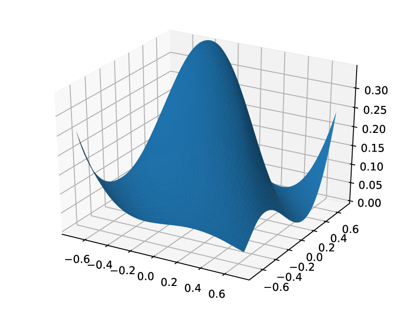
(a) $I=10$.

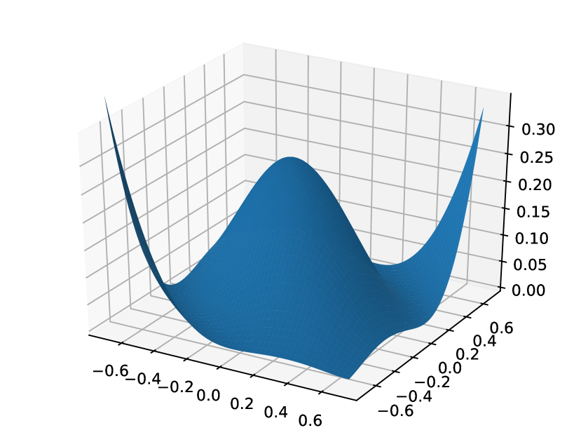
(b) $I=30$.

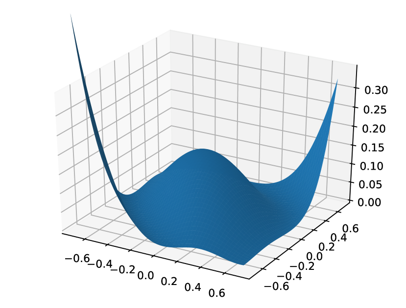
(c) $I=70$.

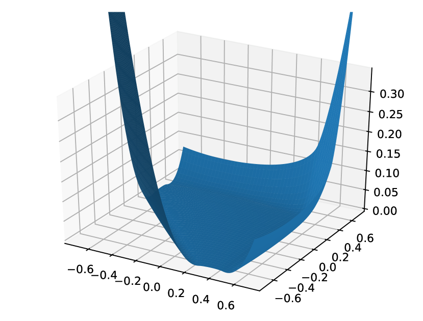
(d) $I=1,000$.

Figure 1: The loss surface of one-hidden-layer ReLU network projected onto a 2-d plane, which is spanned by three points to which the SGD algorithm converges according to three different initialization seeds. It shows that as the number of hidden neurons $I$ increases, the landscape becomes less non-convex.

Our Contributions. This paper provides both theoretical and experimental results for the population and empirical risks of deep neural networks by estimating the duality gap.

First, we study the duality gap of deep neural networks with arbitrary activation functions, adversarial data distribution, and multi-branch architecture (see Theorem 1). The multi-branch architecture is general, which includes the classic one-hidden-layer architecture as a special case (see Figure 2). By Shapley-Folkman lemma, we show that the duality gap of both population and empirical risks shrinks to zero as the number of branches increases. Our result provides better understanding of various state-of-the-art architectures such as ResNeXt, Inception, Xception, SqueezeNet, and Wide ResNet.

Second, we prove that the strong duality (a.k.a. zero duality gap) holds for the empirical risk of deep linear neural networks (see Theorem 2). To this end, we develop multiple new proof techniques, including reduction to low-rank approximation and construction of dual certificate (see Section 4).

Finally, we empirically study the loss surface of multi-branch neural networks. Our experiments verify our theoretical findings.

Notation. We will use bold capital letter to represent matrix and lower-case letter to represent scalar. Specifically, let $\mathbf{I}$ be the identity matrix and denote by $\mathbf{0}$ the all-zero matrix. Let $\{\mathbf{W}_{i}\in\mathbb{R}^{d_{i}\times d_{i-1}}:i=1,2,...,H\}$ be a set of network parameters, each of which represents the connection weights between the $i$-th and $(i+1)$-th layers of neural network. We use $\mathbf{W}_{:,t}\in\mathbb{R}^{n_{1}\times 1}$ to indicate the $t$-th column of $\mathbf{W}$. We will use $\sigma_{i}(\mathbf{W})$ to represent the $i$-th largest singular value of matrix $\mathbf{W}$. Given skinny SVD $\mathbf{U}\bm{\Sigma}\mathbf{V}^{T}$ of matrix $\mathbf{W}$, we denote by $\textup{{svd}}_{r}(\mathbf{W})=\mathbf{U}_{:,1:r}\bm{\Sigma}_{1:r,1:r}\mathbf{V}_{:,1:r}^{T}$ the truncated SVD of $\mathbf{W}$ to the first $r$ singular values. For matrix norms, denote by $\|\mathbf{W}\|_{\mathcal{S}_{H}}=\left(\sum_{i}\sigma_{i}^{H}(\mathbf{W})\right)^{1/H}$ the matrix Schatten-$H$ norm. Nuclear norm and Frobenius norm are special cases of Schatten-$H$ norm: $\|\mathbf{W}\|_{*}=\|\mathbf{W}\|_{\mathcal{S}_{1}}$ and $\|\mathbf{W}\|_{F}=\|\mathbf{W}\|_{\mathcal{S}_{2}}$. We use $\|\mathbf{W}\|$ to represent the matrix operator norm, i.e., $\|\mathbf{W}\|=\sigma_{1}(\mathbf{W})$, and denote by $\textup{{rank}}(\mathbf{W})$ the rank of matrix $\mathbf{W}$. Denote by $\mathsf{Row}(\mathbf{W})$ the span of rows of $\mathbf{W}$. Let $\mathbf{W}^{\dagger}$ be the Moore-Penrose pseudo-inverse of $\mathbf{W}$.

For convex matrix function $K(\cdot)$, we denote by $K^{*}(\mathbf{\Lambda})=\max_{\mathbf{M}}\langle\mathbf{\Lambda},\mathbf{M}\rangle-K(\mathbf{M})$ the conjugate function of $K(\cdot)$ and $\partial K(\cdot)$ the sub-differential. We use $\textup{{diag}}(\sigma_{1},...,\sigma_{r})$ to represent a $r\times r$ diagonal matrix with diagonal entries $\sigma_{1},...,\sigma_{r}$. Let $d_{\min}=\min\{d_{i}:i=1,2,...,H-1\}$, and $[I]=\{1,2,...,I\}$. For any two matrices $\mathbf{A}$ and $\mathbf{B}$ of matching dimensions, we denote by $[\mathbf{A},\mathbf{B}]$ the concatenation of $\mathbf{A}$ and $\mathbf{B}$ along the row and $[\mathbf{A};\mathbf{B}]$ the concatenation of two matrices along the column.

2 Duality Gap of Multi-Branch Neural Networks

We first study the duality gap of neural networks in a classification setting. We show that the wider the network is, the smaller the duality gap becomes.

Network Setup. The output of our network follows from a multi-branch architecture (see Figure 2):

$$f(\mathbf{w};\mathbf{x})=\frac{1}{I}\sum_{i=1}^{I}f_{i}(\mathbf{w}_{(i)};\mathbf{x}),\quad\mathbf{w}_{(i)}\in\mathcal{W}_{i},\quad(\mathcal{W}_{i}\text{ is convex set})$$

where $\mathbf{w}$ is the concatenation of all network parameters $\{\mathbf{w}_{(i)}\}_{i=1}^{I}$, $\mathbf{x}\in\mathbb{R}^{d_{0}}$ is the input instance, $\{\mathcal{W}_{i}\}_{i=1}^{I}$ is the parameter space, and $f_{i}(\mathbf{w}_{(i)};\cdot)$ represents an $\mathbb{R}^{d_{0}}\rightarrow\mathbb{R}$ continuous mapping by a sub-network which is allowed to have arbitrary architecture such as convolutional and recurrent neural networks. As an example, $f_{i}(\mathbf{w}_{(i)};\cdot)$ can be in the form of a $H_{i}$-layer feed-forward sub-network:

$$f_{i}(\mathbf{w}_{(i)};\mathbf{x})=\mathbf{w}_{i}^{\top}\psi_{H_{i}}(\mathbf{W}_{H_{i}}^{(i)}...\psi_{1}(\mathbf{W}_{1}^{(i)}\mathbf{x}))\in\mathbb{R},\ \mathbf{w}_{(i)}=[\mathbf{w}_{i};\mathsf{vec}(\mathbf{W}_{1}^{(i)});...;\mathsf{vec}(\mathbf{W}_{H_{i}}^{(i)})]\in\mathbb{R}^{p_{i}}.$$

Hereby, the functions $\psi_{k}(\cdot),k=1,2,...,H_{i}$ are allowed to encode arbitrary form of continuous element-wise non-linearity (and linearity) after each matrix multiplication, such as sigmoid, rectification, convolution, while the number of layers $H_{i}$ in each sub-network can be arbitrary as well. When $H_{i}=1$ and $d_{H_{i}}=1$, i.e., each sub-network in Figure 2 represents one hidden unit, the architecture $f(\mathbf{w};\mathbf{x})$ reduces to a one-hidden-layer network. We apply the so-called $\tau$-hinge loss [4, 7] on the top of network output for label $y\in\{-1,+1\}$:

$$\ell_{\tau}(\mathbf{w};\mathbf{x},y):=\max\left(0,1-\frac{y\cdot f(\mathbf{w};\mathbf{x})}{\tau}\right),\quad\tau>0.$$ (1)

The $\tau$-hinge loss has been widely applied in active learning of classifiers and margin based learning [4, 7]. When $\tau=1$, it reduces to the classic hinge loss [43, 17, 38].

We make the following assumption on the margin parameter $\tau$, which states that the parameter $\tau$ is sufficiently large.

Assumption 1 (Parameter $\tau$).

For sample $(\mathbf{x},y)$ drawn from distribution $\mathcal{P}$, we have $\tau>y\cdot f(\mathbf{w};\mathbf{x})$ for all $\mathbf{w}\in\mathcal{W}_{1}\times\mathcal{W}_{2}\times...\times\mathcal{W}_{I}$ with probability measure $1$.

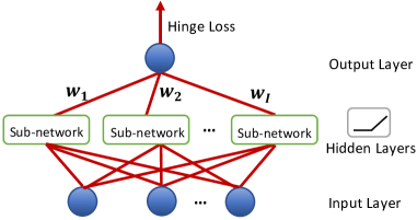
Figure 2: Multi-branch architecture, where the sub-networks are allowed to have arbitrary architectures, depths, and continuous activation functions. In the extreme case when the sub-network is chosen to have a single neuron, the multi-branch architecture reduces to a single-hidden-layer neural network.

We further empirically observe that using smaller values of the parameter $\tau$ and other loss functions support our theoretical result as well (see experiments in Section 5). It is an interesting open question to extend our theory to more general losses in the future.

To study how close these generic neural network architectures approach the family of convex functions, we analyze the duality gap of minimizing the risk w.r.t. the loss (1) with an extra regularization constraint. The normalized duality gap is a measure of intrinsic non-convexity of a given function [13]: the gap is zero when the given function itself is convex, and is large when the loss surface is far from the convexity intrinsically. Typically, the closer the network approaches to the family of convex functions, the easier we can optimize the network.

Multi-Branch Architecture. Our analysis of multi-branch neural networks is built upon tools from non-convex geometric analysis — Shapley–Folkman lemma. Basically, the Shapley–Folkman lemma states that the sum of constrained non-convex functions is close to being convex. A neural network is an ideal target to apply this lemma to: the width of network is associated with the number of summand functions. So intuitively, the wider the neural network is, the smaller the duality gap will be. In particular, we study the following non-convex problem concerning the population risk:

$$\min_{\mathbf{w}\in\mathcal{W}_{1}\times...\times\mathcal{W}_{I}}\mathbb{E}_{(\mathbf{x},y)\sim\mathcal{P}}[\ell_{\tau}(\mathbf{w};\mathbf{x},y)],\ \ \mbox{s.t.}\ \ \frac{1}{I}\sum_{i=1}^{I}h_{i}(\mathbf{w}_{(i)})\leq K,$$ (2)

where $h_{i}(\cdot),i\in[I]$ are convex regularization functions, e.g., the weight decay, and $K$ can be arbitrary such that the problem is feasible. Correspondingly, the dual problem of problem (2) is a one-dimensional convex optimization problem:

$$\begin{split}\max_{\lambda\geq 0}\mathcal{Q}(\lambda)-\lambda K,\quad\textup{where }\mathcal{Q}(\lambda):=\inf_{\mathbf{w}\in\mathcal{W}_{1}\times...\times\mathcal{W}_{I}}\mathbb{E}_{(\mathbf{x},y)\sim\mathcal{P}}[\ell_{\tau}(\mathbf{w};\mathbf{x},y)]+\frac{\lambda}{I}\sum_{i=1}^{I}h_{i}(\mathbf{w}_{(i)}).\end{split}$$ (3)

For $\widetilde{\mathbf{w}}\in\mathcal{W}_{i}$, denote by

$$\widetilde{f}_{i}(\widetilde{\mathbf{w}}):=\inf_{a^{j},\mathbf{w}_{(i)}^{j}\in\mathcal{W}_{i}}\left\{\sum_{j=1}^{p_{i}+1}a^{j}\mathbb{E}_{(\mathbf{x},y)\sim\mathcal{P}}\left(1-\frac{y\cdot f_{i}(\mathbf{w}_{(i)}^{j};\mathbf{x})}{\tau}\right):\widetilde{\mathbf{w}}=\sum_{j=1}^{p_{i}+1}a^{j}\mathbf{w}_{(i)}^{j},\sum_{j=1}^{p_{i}+1}a^{j}=1,a^{j}\geq 0\right\}$$

the convex relaxation of function $\mathbb{E}_{(\mathbf{x},y)\sim\mathcal{P}}[1-y\cdot f_{i}(\cdot;\mathbf{x})/\tau]$ on $\mathcal{W}_{j}$. For $\widetilde{\mathbf{w}}\in\mathcal{W}_{i}$, we also define

$$\widehat{f}_{i}(\widetilde{\mathbf{w}}):=\inf_{\mathbf{w}_{(i)}\in\mathcal{W}_{i}}\left\{\mathbb{E}_{(\mathbf{x},y)\sim\mathcal{P}}\left(1-\frac{y\cdot f_{i}(\mathbf{w}_{(i)};\mathbf{x})}{\tau}\right):h_{i}(\mathbf{w}_{(i)})\leq h_{i}(\widetilde{\mathbf{w}})\right\}.$$

Our main results for multi-branch neural networks are as follows:

Theorem 1.

Denote by $\inf(\mathbf{P})$ the minimum of primal problem (2) and $\sup(\mathbf{D})$ the maximum of dual problem (3). Let $\Delta_{i}:=\sup_{\mathbf{w}\in\mathcal{W}_{i}}\left\{\widehat{f}_{i}(\mathbf{w})-\widetilde{f}_{i}(\mathbf{w})\right\}\geq 0$ and $\Delta_{worst}:=\max_{i\in[I]}\Delta_{i}$. Suppose $\mathcal{W}_{i}$’s are compact and both $f_{i}(\mathbf{w}_{(i)};\mathbf{x})$ and $h_{i}(\mathbf{w}_{(i)})$ are continuous w.r.t. $\mathbf{w}_{(i)}$. If there exists at least one feasible solution of problem (P), then under Assumption 1 the duality gap w.r.t. problems (2) and (3) can be bounded by

$$0\leq\frac{\inf(\mathbf{P})-\sup(\mathbf{D})}{\Delta_{worst}}\leq\frac{2}{I}.$$

Note that $\Delta_{i}$ measures the divergence between the function value of $\widehat{f}_{i}$ and its convex relaxation $\widetilde{f}_{i}$. The constant $\Delta_{worst}$ is the maximal divergence among all sub-networks, which grows slowly with the increase of $I$. This is because $\Delta_{worst}$ only measures the divergence of one branch. The normalized duality gap $(\inf(\mathbf{P})-\sup(\mathbf{D}))/\Delta_{worst}$ has been widely used before to measure the degree of non-convexity of optimization problems [13, 58, 14, 24, 22]. Such a normalization avoids trivialities in characterizing the degree of non-convexity: scaling the objective function by any constant does not change the value of normalized duality gap. Even though Theorem 1 is in the form of population risk, the conclusion still holds for the empirical loss as well. This can be achieved by setting the marginal distribution $\mathcal{P}_{\mathbf{x}}$ as the uniform distribution on a finite set and $\mathcal{P}_{y}$ as the corresponding labels uniformly distributed on the same finite set.

Inspiration for Architecture Designs. Theorem 1 shows that the loss surface of deep network is less non-convex when the width $I$ is large; when $I\rightarrow+\infty$, surprisingly, deep network is as easy as a convex optimization. An intuitive explanation is that the large number of randomly initialized hidden units represent all possible features. Thus the optimization problem involves just training the top layer of the network, which is convex. Our result encourages a class of network architectures with multiple branches and supports some of the most successful architectures in practice, such as Inception [57], Xception [18], ResNeXt [63], SqueezeNet [33], Wide ResNet [64], Shake-Shake regularization [25] — all of which benefit from the split-transform-merge behaviour as shown in Figure 2. The theory sheds light on an explanation of strong performance of these architectures.

Related Works. While many efforts have been devoted to studying the local minima or saddle points of deep neural networks [42, 68, 55, 36, 62, 61], little is known about the duality gap of deep networks. In particular, Choromanska et al. [20, 19] showed that the number of poor local minima cannot be too large. Kawaguchi [35] improved over the results of [20, 19] by assuming that the activation functions are independent Bernoulli variables and the input data are drawn from Gaussian distribution. Xie et al. [62] and Haeffele et al. [30] studied the local minima of regularized network, but they require either the network is shallow, or the network weights are rank-deficient. Ge et al. [27] showed that every local minimum is globally optimal by modifying the activation function. Zhang et al. [67] and Aslan et al. [3] reduced the non-linear activation to the linear case by kernelization and relaxed the non-convex problem to a convex one. However, no formal guarantee was provided for the tightness of the relaxation. Theorem 1, on the other hand, bounds the duality gap of deep neural networks with mild assumptions.

Another line of research studies the convexity behaviour of neural networks when the number of hidden neurons goes to the infinity. In particular, Bach [5] proved that a single-hidden-layer network is as easy as a convex optimization by using classical non-Euclidean regularization tools. Bengio et al. [12] showed a similar phenomenon for multi-layer networks with an incremental algorithm. In comparison, Theorem 1 not only captures the convexification phenomenon when $I\rightarrow+\infty$, but also goes beyond the result as it characterizes the convergence rate of convexity of neural networks in terms of duality gap. Furthermore, the conclusion in Theorem 1 holds for the population risk, which was unknown before.

3 Strong Duality of Linear Neural Networks

In this section, we show that the duality gap is zero if the activation function is linear. Deep linear neural network has received significant attention in recent years [51, 35, 67, 44, 8, 28, 31, 9] because of its simple formulation and its connection to non-linear neural networks.

Network Setup. We discuss the strong duality of regularized deep linear neural networks of the form

$$(\mathbf{W}_{1}^{*},...,\mathbf{W}_{H}^{*})=\operatorname*{argmin}_{\mathbf{W}_{1},...,\mathbf{W}_{H}}\frac{1}{2}\|\mathbf{Y}-\mathbf{W}_{H}\cdots\mathbf{W}_{1}\mathbf{X}\|_{F}^{2}+\frac{\gamma}{H}\left[\|\mathbf{W}_{1}\mathbf{X}\|_{\mathcal{S}_{H}}^{H}+\sum_{i=2}^{H}\|\mathbf{W}_{i}\|_{\mathcal{S}_{H}}^{H}\right],$$ (4)

where $\mathbf{X}=[\mathbf{x}_{1},...,\mathbf{x}_{n}]\in\mathbb{R}^{d_{0}\times n}$ is the given instance matrix, $\mathbf{Y}=[\mathbf{y}_{1},...,\mathbf{y}_{n}]\in\mathbb{R}^{d_{H}\times n}$ is the given label matrix, and $\mathbf{W}_{i}\in\mathbb{R}^{d_{i}\times d_{i-1}},i\in[I]$ represents the weight matrix in each linear layer. We mention that (a) while the linear operation is simple matrix multiplications in problem (4), it can be easily extended to other linear operators, e.g., the convolutional operator or the linear operator with the bias term, by properly involving a group of kernels in the variable $\mathbf{W}_{i}$ [30]. (b) The regularization terms in problem (4) are of common interest, e.g., see [30]. When $H=2$, our regularization terms reduce to $\frac{1}{2}\|\mathbf{W}_{i}\|_{F}^{2}$, which is well known as the weight-decay or Tikhonov regularization. (c) The regularization parameter $\gamma$ is the same for each layer since we have no further information on the preference of layers.

Our analysis leads to the following guarantees for the deep linear neural networks.

Theorem 2.

Denote by $\widetilde{\mathbf{Y}}:=\mathbf{Y}\mathbf{X}^{\dagger}\mathbf{X}\in\mathbb{R}^{d_{H}\times n}$ and $d_{\min}:=\min\{d_{1},...,d_{H-1}\}\leq\min\{d_{0},d_{H},n\}$. Let $0\leq\gamma<\sigma_{\min}(\widetilde{\mathbf{Y}})$ and $H\geq 2$, where $\sigma_{\min}(\widetilde{\mathbf{Y}})$ stands for the minimal non-zero singular value of $\widetilde{\mathbf{Y}}$. Then the strong duality holds for deep linear neural network (4). In other words, the optimum of problem (4) is the same as its convex dual problem

$$\mathbf{\Lambda}^{*}=\operatorname*{argmax}_{\mathsf{Row}(\mathbf{\Lambda})\subseteq\mathsf{Row}(\mathbf{X})}-\frac{1}{2}\|\widetilde{\mathbf{Y}}-\mathbf{\Lambda}\|_{d_{\min}}^{2}+\frac{1}{2}\|\mathbf{Y}\|_{F}^{2},\quad\textup{s.t.}\quad\|\mathbf{\Lambda}\|\leq\gamma,$$ (5)

where $\|\cdot\|_{d_{\min}}^{2}=\sum_{i=1}^{d_{\min}}\sigma_{i}^{2}(\cdot)$ is a convex function. Moreover, the optimal solutions of primal problem (4) can be obtained from the dual problem (5) in the following way: let $\mathbf{U}\bm{\Sigma}\mathbf{V}^{T}=\textup{{svd}}_{d_{\min}}(\widetilde{\mathbf{Y}}-\mathbf{\Lambda}^{*})$ be the skinny SVD of matrix $\textup{{svd}}_{d_{\min}}(\widetilde{\mathbf{Y}}-\mathbf{\Lambda}^{*})$, then $\mathbf{W}_{i}^{*}=[\bm{\Sigma}^{1/H},\mathbf{0};\mathbf{0},\mathbf{0}]\in\mathbb{R}^{d_{i}\times d_{i-1}}$ for $i=2,3,...,H-1$, $\mathbf{W}_{H}^{*}=[\mathbf{U}\bm{\Sigma}^{1/H},\mathbf{0}]\in\mathbb{R}^{d_{H}\times d_{H-2}}$ and $\mathbf{W}_{1}^{*}=[\bm{\Sigma}^{1/H}\mathbf{V}^{T};\mathbf{0}]\mathbf{X}^{\dagger}\in\mathbb{R}^{d_{1}\times d_{0}}$ is a globally optimal solution to problem (4).

The regularization parameter $\gamma$ cannot be too large in order to avoid underfitting. Our result provides a suggested upper bound $\sigma_{\min}(\widetilde{\mathbf{Y}})$ for the regularization parameter, where oftentimes $\sigma_{\min}(\widetilde{\mathbf{Y}})$ characterizes the level of random noise. When $\gamma=0$, our analysis reduces to the un-regularized deep linear neural network, a model which has been widely studied in [35, 44, 8, 28].

Theorem 2 implies the followig result on the landscape of deep linear neural networks: the regularized deep learning can be converted into an equivalent convex problem by dual. We note that the strong duality rarely happens in the non-convex optimization: matrix completion [6], Fantope [48], and quadratic optimization with two quadratic constraints [11] are among the few paradigms that enjoy the strong duality. For deep networks, the effectiveness of convex relaxation has been observed empirically in [3, 67], but much remains unknown for the theoretical guarantees of the relaxation. Our work shows strong duality of regularized deep linear neural networks and provides an alternative approach to overcome the computational obstacles due to the non-convexity: one can apply convex solvers, e.g., the Douglas–Rachford algorithm, for problem (5) and then conduct singular value decomposition to compute the weights $\{\mathbf{W}_{i}^{*}\}_{i=1}^{H}$ from $\textup{{svd}}_{d_{\min}}(\widetilde{\mathbf{Y}}-\mathbf{\Lambda}^{*})$. In addition, our result inherits the benefits of convex analysis. The vast majority results on deep learning study the generalization error or expressive power by analyzing its complicated non-convex form [47, 66, 65]. In contrast, with strong duality one can investigate various properties of deep linear networks with much simpler convex form.

Related Works. The goal of convexified linear neural networks is to relax the non-convex form of deep learning to the computable convex formulations [67, 3]. While several efforts have been devoted to investigating the effectiveness of such convex surrogates, e.g., by analyzing the generalization error after the relaxation [67], little is known whether the relaxation is tight to its original problem. Our result, on the other hand, provides theoretical guarantees for the tightness of convex relaxation of deep linear networks, a phenomenon observed empirically in [3, 67].

We mention another related line of research — no bad local minima. On one hand, although recent works have shown the absence of spurious local minimum for deep linear neural networks [50, 35, 44], many of them typically lack theoretical analysis of regularization term. Specifically, Kawaguchi [35] showed that un-regularized deep linear neural networks have no spurious local minimum. Lu and Kawaguchi [44] proved that depth creates no bad local minimum for un-regularized deep linear neural networks. In contrast, our optimization problem is more general by taking the regularization term into account. On the other hand, even the “local=global” argument holds for the deep linear neural networks, it is still hard to escape bad saddle points [1]. In particular, Kawaguchi [35] proved that for linear networks deeper than three layers, there exist bad saddle points at which the Hessian does not have any negative eigenvalue. Therefore, the state-of-the-art algorithms designed to escape the saddle points might not be applicable [34, 26]. Our result provides an alternative approach to solve deep linear network by convex programming, which bypasses the computational issues incurred by the bad saddle points.

4 Our Techniques and Proof Sketches

In this section, we present our techniques and proof sketches of Theorems 1 and 2.

(a) Shapley-Folkman Lemma. The proof of Theorem 1 is built upon the Shapley-Folkman lemma [22, 56, 24, 13], which characterizes a convexification phenomenon concerning the average of multiple sets and is analogous to the central limit theorem in the probability theory. Consider the averaged Minkowski sum of $I$ sets $\mathcal{A}_{1},\mathcal{A}_{2},...,\mathcal{A}_{I}$ given by $\{I^{-1}\sum_{j\in[I]}a_{j}:a_{j}\in\mathcal{A}_{j}\}$. Intuitively, the lemma states that $\rho(I^{-1}\sum_{j\in[I]}\mathcal{A}_{j})\rightarrow 0$ as $I\rightarrow+\infty$, where $\rho(\cdot)$ is a metric of the non-convexity of a set (see Figure 3 for visualization). We apply this lemma to the optimization formulation of deep neural networks. Denote by augmented epigraph the set $\{(h(\mathbf{w}),\ell(\mathbf{w})):\text{all possible choices of }\mathbf{w}\}$, where $h$ is the constraint and $\ell$ is the objective function in the optimization problem. The key observation is that the augmented epigraph of neural network loss with multi-branch architecture can be expressed as the Minkowski average of augmented epigraphs of all branches. Thus we obtain a natural connection between an optimization problem and its corresponding augmented epigraph. Applying Shapley-Folkman lemma to the augmented epigraph leads to a characteristic of non-convexity of the deep neural network.

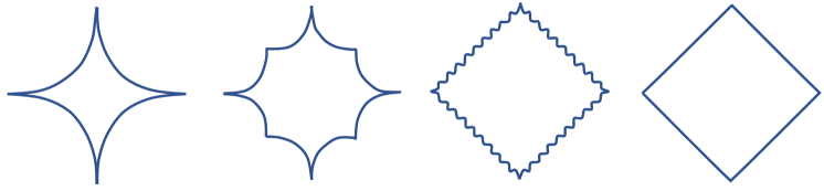
Figure 3: Visualization of Shapley-Folkman lemma. The first figure: an $\ell_{1/2}$ ball. The second and third figures: the averaged Minkowski sum of two and ten $\ell_{1/2}$ balls. The fourth figure: the convex hull of $\ell_{1/2}$ ball (the Minkowski average of infinitely many $\ell_{1/2}$ balls). It show that with the number of $\ell_{1/2}$ balls to be averaged increasing, the Minkowski average tends to be more convex.

(b) Variational Form. The proof of Theorem 2 is built upon techniques (b), (c), and (d). In particular, problem (4) is highly non-convex due to its multi-linear form over the optimized variables $\{\mathbf{W}_{i}\}_{i=1}^{H}$. Fortunately, we are able to analyze the problem by grouping $\mathbf{W}_{H}\mathbf{W}_{H-1}...\mathbf{W}_{1}\mathbf{X}$ together and converting the original non-convex problem in terms of the separate variables $\{\mathbf{W}_{i}\}_{i=1}^{H}$ to a convex optimization with respect to the new grouping variable $\mathbf{W}_{H}\mathbf{W}_{H-1}...\mathbf{W}_{1}\mathbf{X}$. This typically requires us to represent the objective function of (4) as a convex function of $\mathbf{W}_{H}\mathbf{W}_{H-1}...\mathbf{W}_{1}$. To this end, we prove that $\|\mathbf{W}_{H}\mathbf{W}_{H-1}...\mathbf{W}_{1}\mathbf{X}\|_{*}=\min_{\mathbf{W}_{1},...,\mathbf{W}_{H}}\displaystyle\frac{1}{H}\left[\|\mathbf{W}_{1}\mathbf{X}\|_{\mathcal{S}_{H}}^{H}+\sum_{i=2}^{H}\|\mathbf{W}_{i}\|_{\mathcal{S}_{H}}^{H}\right]$ (see Lemma 4 in Appendix C). So the objective function in problem (4) has an equivalent form

$$\min_{\mathbf{W}_{1},...,\mathbf{W}_{H}}\frac{1}{2}\|\mathbf{Y}-\mathbf{W}_{H}\mathbf{W}_{H-1}\cdots\mathbf{W}_{1}\mathbf{X}\|_{F}^{2}+\gamma\|\mathbf{W}_{H}\mathbf{W}_{H-1}\cdots\mathbf{W}_{1}\mathbf{X}\|_{*}.$$ (6)

This observation enables us to represent the optimization problem as a convex function of the output of a neural network. Therefore, we can analyze the non-convex problem by applying powerful tools from convex analysis.

(c) Reduction to Low-Rank Approximation. Our results of strong duality concerning problem (6) are inspired by the problem of low-rank matrix approximation:

$$\min_{\mathbf{W}_{1},...,\mathbf{W}_{H}}\frac{1}{2}\|\mathbf{Y}-\mathbf{\Lambda}^{*}-\mathbf{W}_{H}\mathbf{W}_{H-1}\cdots\mathbf{W}_{1}\mathbf{X}\|_{F}^{2}.$$ (7)

We know that all local solutions of (7) are globally optimal [35, 44, 6]. To analyze the more general regularized problem (4), our main idea is to reduce problem (6) to the form of (7) by Lagrangian function. In other words, the Lagrangian function of problem (6) should be of the form (7) for a fixed Lagrangian variable $\mathbf{\Lambda}^{*}$, which we will construct later in subsection (d). While some prior works attempted to apply a similar reduction, their conclusions either depended on unrealistic conditions on local solutions, e.g., all local solutions are rank-deficient [30, 29], or their conclusions relied on strong assumptions on the objective functions, e.g., that the objective functions are twice-differentiable [30], which do not apply to the non-smooth problem (6). Instead, our results bypass these obstacles by formulating the strong duality of problem (6) as the existence of a dual certificate $\mathbf{\Lambda}^{*}$ satisfying certain dual conditions (see Lemma 6 in Appendix C). Roughly, the dual conditions state that the optimal solution $(\mathbf{W}_{1}^{*},\mathbf{W}_{2}^{*},...,\mathbf{W}_{H}^{*})$ of problem (6) is locally optimal to problem (7). On one hand, by the above-mentioned properties of problem (7), $(\mathbf{W}_{1}^{*},...,\mathbf{W}_{H}^{*})$ globally minimizes the Lagrangian function when $\mathbf{\Lambda}$ is fixed to $\mathbf{\Lambda}^{*}$. On the other hand, by the convexity of nuclear norm, for the fixed $(\mathbf{W}_{1}^{*},...,\mathbf{W}_{H}^{*})$ the Lagrangian variable $\mathbf{\Lambda}^{*}$ globally optimize the Lagrangian function. Thus $(\mathbf{W}_{1}^{*},...,\mathbf{W}_{H}^{*},\mathbf{\Lambda}^{*})$ is a primal-dual saddle point of the Lagrangian function of problem (6). The desired strong duality is a straightforward result from this argument.

(d) Dual Certificate. The remaining proof is to construct a dual certificate $\mathbf{\Lambda}^{*}$ such that the dual conditions hold true. The challenge is that the dual conditions impose several constraints simultaneously on the dual certificate (see condition (19) in Appendix C), making it hard to find a desired certificate. This is why progress on the dual certificate has focused on convex programming. To resolve the issue, we carefully choose the certificate as an appropriate scaling of subgradient of nuclear norm around a low-rank solution, where the nuclear norm follows from our regularization term in technique (b). Although the nuclear norm has infinitely many subgradients, we prove that our construction of dual certificate obeys all desired dual conditions. Putting techniques (b), (c), and (d) together, our proof of strong duality is completed.

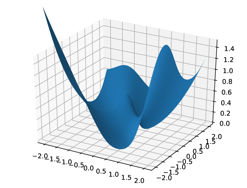
(a) $I=1$.

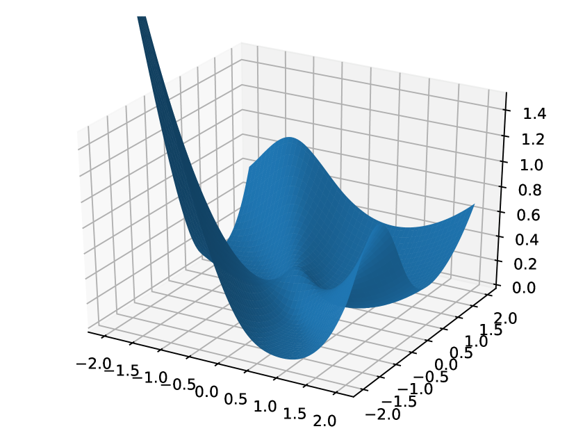
(b) $I=3$.

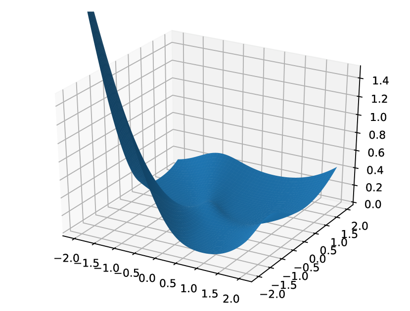
(c) $I=5$.

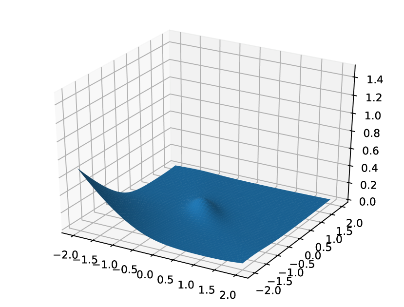
(d) $I=100$.

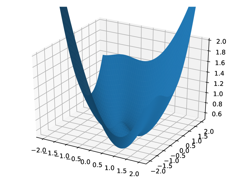
(e) $I=1$.

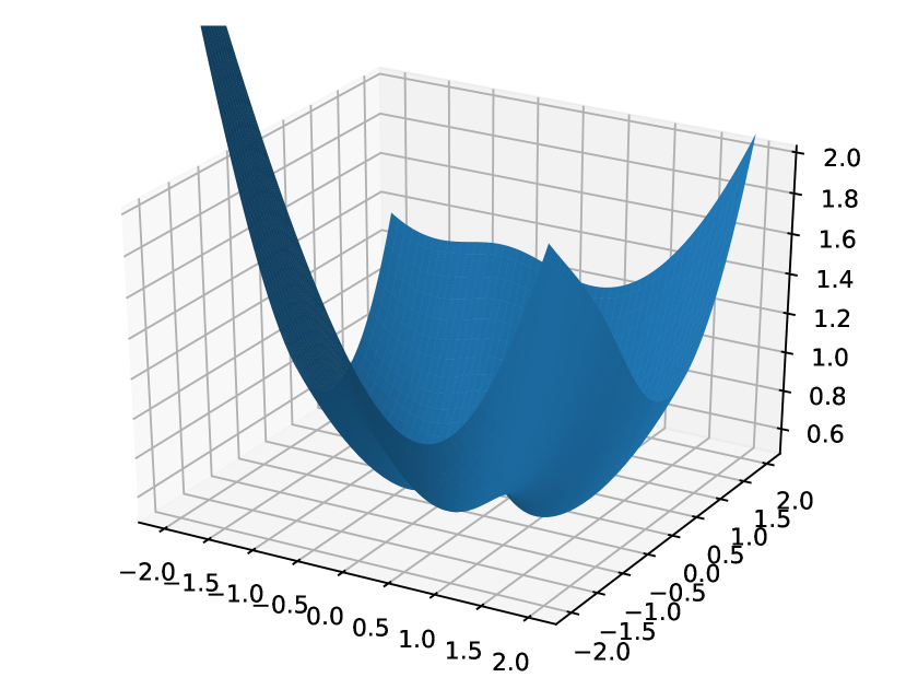
(f) $I=3$.

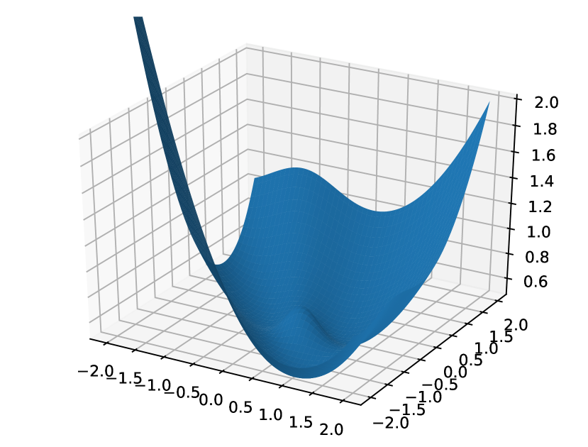
(g) $I=5$.

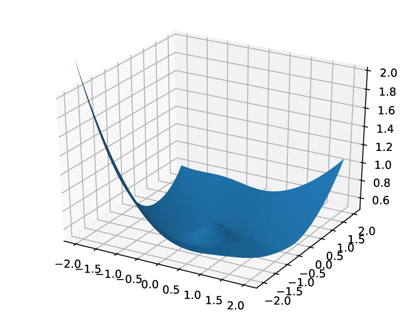
(h) $I=100$.

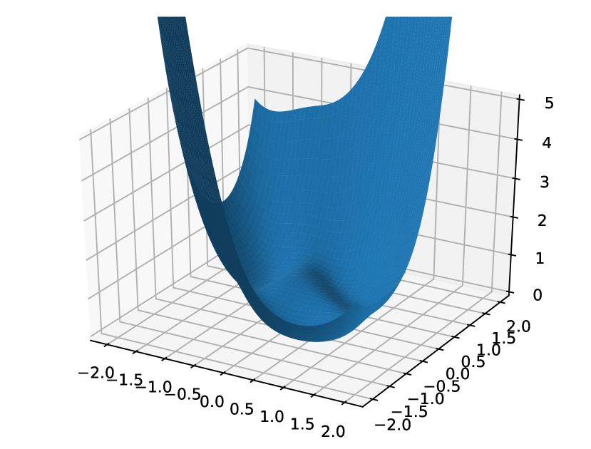
(i) $I=1$.

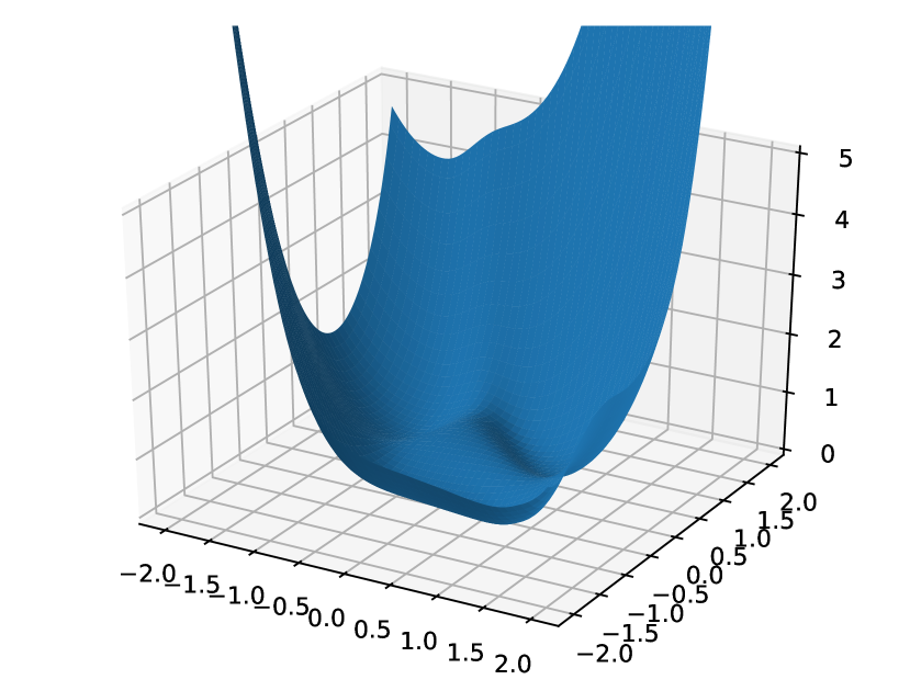
(j) $I=3$.

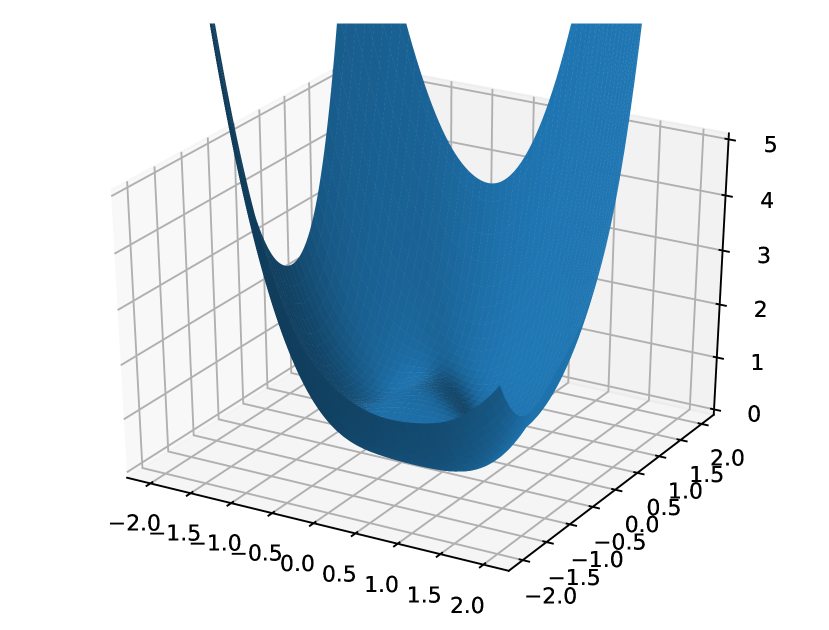
(k) $I=5$.

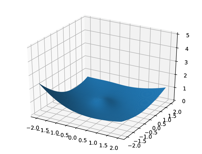
(l) $I=50,000$.

Figure 4: Top Row: Landscape of one-hidden-layer network on MNIST. Middle Row: Landscape of one-hidden-layer network on CIFAR-10. Bottom Row: Landscape of three-hidden-layer, multi-branch network on CIFAR-10 dataset. From left to right, the landscape looks less non-convex.

5 Experiments

In this section, we verify our theoretical contributions by the experimental validation. We release our PyTorch code at https://github.com/hongyanz/multibranch.

5.1 Visualization of Loss Landscape

Experiments on Synthetic Datasets. We first show that over-parametrization results in a less non-convex loss surface for a synthetic dataset. The dataset consists of $1,000$ examples in $\mathbb{R}^{10}$ whose labels are generated by an underlying one-hidden-layer ReLU network $f(\mathbf{x})=\sum_{i=1}^{I}\mathbf{w}_{i,2}^{*}[\mathbf{W}_{i,1}^{*}\mathbf{x}]_{+}$ with 11 hidden neurons [49]. We make use of the visualization technique employed by [40] to plot the landscape, where we project the high-dimensional hinge loss ($\tau=1$) landscape onto a 2-d plane spanned by three points. These points are found by running the SGD algorithm with three different initializations until the algorithm converges. As shown in Figure 1, the landscape exhibits strong non-convexity with lots of local minima in the under-parameterized case $I=10$. But as $I$ increases, the landscape becomes more convex. In the extreme case, when there are $1,000$ hidden neurons in the network, no non-convexity can be observed on the landscape.

Experiments on MNIST and CIFAR-10. We next verify the phenomenon of over-parametrization on MNIST [39] and CIFAR-10 [37] datasets. For both datasets, we follow the standard preprocessing step that each pixel is normalized by subtracting its mean and dividing by its standard deviation. We do not apply data augmentation. For MNIST, we consider a single-hidden-layer network defined as: $f(\mathbf{x})=\sum_{i=1}^{I}\mathbf{W}_{i,2}[\mathbf{W}_{i,1}\mathbf{x}]_{+}$, where $\mathbf{W}_{i,1}\in\mathbb{R}^{h\times d}$, $\mathbf{W}_{i,2}\in\mathbb{R}^{10\times h}$, $d$ is the input dimension, $h$ is the number of hidden neurons, and $I$ is the number of branches, with $d=784$ and $h=8$. For CIFAR-10, in addition to considering the exact same one-hidden-layer architecture, we also test a deeper network containing $3$ hidden layers of size $8$-$8$-$8$, with ReLU activations and $d=3,072$. We apply 10-class hinge loss on the top of the output of considered networks.

Figure 4 shows the changes of landscapes when $I$ increases from $1$ to $100$ for MNIST, and from $1$ to $50,000$ for CIFAR-10, respectively. When there is only one branch, the landscapes have strong non-convexity with many local minima. As the number of branches $I$ increases, the landscape becomes more convex. When $I=100$ for $1$-hidden-layer networks on MNIST and CIFAR-10, and $I=50,000$ for $3$-hidden-layer network on CIFAR-10, the landscape is almost convex.

5.2 Frequency of Hitting Global Minimum

To further analyze the non-convexity of loss surfaces, we consider various one-hidden-layer networks, where each network was trained 100 times using different initialization seeds under the setting discussed in our synthetic experiments of Section 5.1. Since we have the ground-truth global minimum, we record the frequency that SGD hits the global minimum up to a small error $1\times 10^{-5}$ after $100,000$ iterations. Table 1 shows that increasing the number of hidden neurons results in higher hitting rate of global optimality. This further verifies that the loss surface of one-hidden-layer neural network becomes less non-convex as the width increases.

Table 1: Frequency of hitting global minimum by SGD with 100 different initialization seeds.

# Hidden Neurons	Hitting Rate	# Hidden Neurons	Hitting Rate
10	2 / 100	16	30 / 100
11	9 / 100	17	32 / 100
12	21 / 100	18	35 / 100
13	24 / 100	19	52 / 100
14	24 / 100	20	64 / 100
15	29 / 100	21	75 / 100

6 Conclusions

In this work, we study the duality gap for two classes of network architectures. For the neural network with arbitrary activation functions, multi-branch architecture and $\tau$-hinge loss, we show that the duality gap of both population and empirical risks shrinks to zero as the number of branches increases. Our result sheds light on better understanding the power of over-parametrization and the state-of-the-art architectures, where increasing the number of branches tends to make the loss surface less non-convex. For the neural network with linear activation function and $\ell_{2}$ loss, we show that the duality gap is zero. Our two results work for arbitrary depths and adversarial data, while the analytical techniques might be of independent interest to non-convex optimization more broadly.

Acknowledgements. We would like to thank Jason D. Lee for informing us the Shapley-Folkman lemma, and Maria-Florina Balcan, David P. Woodruff, Xiaofei Shi, and Xingyu Xie for their thoughtful comments on the paper.

Appendix A Supplementary Experiments

A.1 Performance of Multi-Branch Architecture

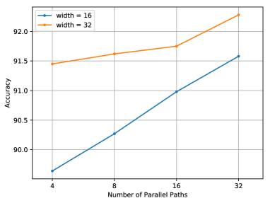
Figure 5: Test accuracy of using VGG-9 as the sub-networks in the multi-branch architecture.

In this section, we test the classification accuracy of the multi-branch architecture on the CIFAR-10 dataset. We use a 9-layer VGG network [53] as our sub-network in each branch, which is memory-efficient for practitioners to fit many branches into GPU memory simultaneously. The detailed network setup of VGG-9 is in Table 2, where the width of VGG-9 is either 16 or 32. We test the performance of varying numbers of branches in the overall architecture from 4 to 32, with cross-entropy loss. Figure 5 presents the test accuracy on CIFAR-10 as the number of branches increases. It shows that the test accuracy improves monotonously with the increasing number of parallel branches/paths.

Table 2: Network architecture of VGG-9. Here $w$ is the width of the network, which controls the number of filters in each convolution layer. All convolution layers have a kernel of size 3, and zero padding of size 1. All layers followed by the batch normalization have no bias term. All max pooling layers have a stride of 2.

Layer	Weight	Activation	Input size	Output size
Input	N / A	N / A	N / A	$3\times 32\times 32$
Conv1	$3\times 3\times 3\times w$	BN + ReLU	$3\times 32\times 32$	$w\times 32\times 32$
Conv2	$3\times 3\times w\times w$	BN + ReLU	$w\times 32\times 32$	$w\times 32\times 32$
MaxPool	N / A	N / A	$w\times 32\times 32$	$w\times 16\times 16$
Conv3	$3\times 3\times w\times 2w$	BN + ReLU	$w\times 16\times 16$	$2w\times 16\times 16$
Conv4	$3\times 3\times 2w\times 2w$	BN + ReLU	$2w\times 16\times 16$	$2w\times 16\times 16$
MaxPool	N / A	N / A	$2w\times 16\times 16$	$2w\times 8\times 8$
Conv5	$3\times 3\times 2w\times 4w$	BN + ReLU	$2w\times 8\times 8$	$4w\times 8\times 8$
Conv6	$3\times 3\times 4w\times 4w$	BN + ReLU	$4w\times 8\times 8$	$4w\times 8\times 8$
Conv7	$3\times 3\times 4w\times 4w$	BN + ReLU	$4w\times 8\times 8$	$4w\times 8\times 8$
MaxPool	N / A	N / A	$4w\times 8\times 8$	$4w\times 4\times 4$
Flatten	N / A	N / A	$4w\times 4\times 4$	$64w$
FC1	$64w\times 4w$	BN + ReLU	$64w$	$4w$
FC2	$4w\times 10$	Softmax	$4w$	$10$

A.2 Strong Duality of Deep Linear Neural Networks

We compare the optima of primal problem (4) and dual problem (5) by numerical experiments for three-layer linear neural networks ($H=3$). The data are generated as follows. We construct the output matrix $\mathbf{Y}\in\mathbb{R}^{100\times 100}$ by drawing the entries of $\mathbf{Y}$ from i.i.d. standard Gaussian distribution and the input matrix $\mathbf{X}\in\mathbb{R}^{100\times 100}$ by the identity matrix. The $d_{\min}$ varies from $5$ to $50$. Both primal and dual problems are solved by numerical algorithms. Given the non-convex nature of primal problem, we rerun the algorithm by multiple initializations and choose the best solution that we obtain. The results are shown in Figure 6. We can easily see that the optima of primal and dual problems almost match. The small gap is due to the numerical inaccuracy.

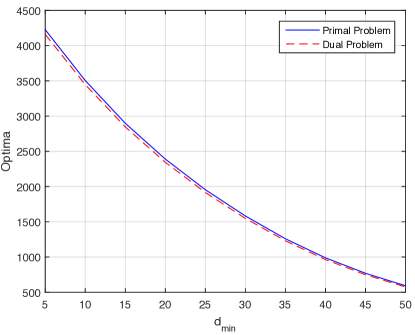
Figure 6: Comparison of optima between primal and dual problems.

We also compare the $\ell_{2}$ distance between the solution $\mathbf{W}_{H}^{*}\mathbf{W}_{H-1}^{*}\ldots\mathbf{W}_{1}^{*}$ of primal problem and the solution $\textup{{svd}}_{d_{\min}}(\widetilde{\mathbf{Y}}-\mathbf{\Lambda}^{*})$ of dual problem in Table 3. We see that the solutions are close to each other.

Table 3: Comparison of the $\ell_{2}$ distance between the solutions of primal and dual problems.

$d_{\min}$	5	10	15	20	25	30	35	40	45	50
$\ell_{2}$ distance ($\times 10^{-10}$)	$1.95$	$1.26$	$7.89$	$3.80$	3.14	1.92	1.04	3.92	6.53	8.00

Appendix B Proofs of Theorem 1: Duality Gap of Multi-Branch Neural Networks

The lower bound $0\leq\frac{\inf(\mathbf{P})-\sup(\mathbf{D})}{\Delta_{worst}}$ is obvious by the weak duality. So we only need to prove the upper bound $\frac{\inf(\mathbf{P})-\sup(\mathbf{D})}{\Delta_{worst}}\leq\frac{2}{I}$.

Consider the subset of $\mathbb{R}^{2}$:

$$\mathcal{Y}_{i}:=\left\{\mathbf{y}_{i}\in\mathbb{R}^{2}:\mathbf{y}_{i}=\frac{1}{I}\left[h_{i}(\mathbf{w}_{(i)}),\mathbb{E}_{(\mathbf{x},y)\sim\mathcal{P}}\left(1-\frac{y\cdot f_{i}(\mathbf{w}_{(i)};\mathbf{x})}{\tau}\right)\right],\mathbf{w}_{(i)}\in\mathcal{W}_{i}\right\},\quad i\in[I].$$

Define the vector summation

$$\mathcal{Y}:=\mathcal{Y}_{1}+\mathcal{Y}_{2}+...+\mathcal{Y}_{I}.$$

Since $f_{i}(\mathbf{w}_{(i)};\mathbf{x})$ and $h_{i}(\mathbf{w}_{(i)})$ are continuous w.r.t. $\mathbf{w}_{(i)}$ and $\mathcal{W}_{i}$’s are compact, the set

$$\{(\mathbf{w}_{(i)},h_{i}(\mathbf{w}_{(i)}),f_{i}(\mathbf{w}_{(i)};\mathbf{x})):\mathbf{w}_{(i)}\in\mathcal{W}_{i}\}$$

is compact as well. So $\mathcal{Y}$, $\mathsf{conv}(\mathcal{Y})$, $\mathcal{Y}_{i}$, and $\mathsf{conv}(\mathcal{Y}_{i})$, $i\in[I]$ are all compact sets. According to the definition of $\mathcal{Y}$ and the standard duality argument [45], we have

$$\inf(\mathbf{P})=\min\left\{w:\mbox{there exists }(r,w)\in\mathcal{Y}\mbox{ such that }r\leq K\right\},$$

and

$$\sup(\mathbf{D})=\min\left\{w:\mbox{there exists }(r,w)\in\mathsf{conv}\left(\mathcal{Y}\right)\mbox{ such that }r\leq K\right\}.$$

Technique (a): Shapley-Folkman Lemma. We are going to apply the following Shapley-Folkman lemma.

Lemma 3 (Shapley-Folkman, [56]).

Let $\mathcal{Y}_{i},i\in[I]$ be a collection of subsets of $\mathbb{R}^{m}$. Then for every $\mathbf{y}\in\mathsf{conv}(\sum_{i=1}^{I}\mathcal{Y}_{i})$, there is a subset $\mathcal{I}(\mathbf{y})\subseteq[I]$ of size at most $m$ such that

$$\mathbf{y}\in\left[\sum_{i\not\in\mathcal{I}(\mathbf{y})}\mathcal{Y}_{i}+\sum_{i\in\mathcal{I}(\mathbf{y})}\mathsf{conv}(\mathcal{Y}_{i})\right].$$

We apply Lemma 3 to prove Theorem 1 with $m=2$. Let $(\overline{r},\overline{w})\in\mathsf{conv}(\mathcal{Y})$ be such that

$$\quad\overline{r}\leq K,\quad\mbox{and}\quad\overline{w}=\sup(\mathbf{D}).$$

Applying the above Shapley-Folkman lemma to the set $\mathcal{Y}=\sum_{i=1}^{I}\mathcal{Y}_{i}$, we have that there are a subset $\overline{\mathcal{I}}\subseteq[I]$ of size $2$ and vectors

$$(\overline{r}_{i},\overline{w}_{i})\in\mathsf{conv}(\mathcal{Y}_{i}),\ \ i\in\overline{\mathcal{I}}\qquad\mbox{and}\qquad\overline{\mathbf{w}}_{(i)}\in\mathcal{W}_{i},\ \ i\not\in\overline{\mathcal{I}},$$

such that

$$\frac{1}{I}\sum_{i\not\in\overline{\mathcal{I}}}h_{i}(\overline{\mathbf{w}}_{(i)})+\sum_{i\in\overline{\mathcal{I}}}\overline{r}_{i}=\overline{r}\leq K,$$ (8)

$$\frac{1}{I}\sum_{i\not\in\overline{\mathcal{I}}}\mathbb{E}_{(\mathbf{x},y)\sim\mathcal{P}}\left(1-\frac{y\cdot f_{i}(\overline{\mathbf{w}}_{(i)};\mathbf{x})}{\tau}\right)+\sum_{i\in\overline{\mathcal{I}}}\overline{w}_{i}=\sup(\mathbf{D}).$$ (9)

Representing elements of the convex hull of $\mathcal{Y}_{i}\subseteq\mathbb{R}^{2}$ by Carathéodory theorem, we have that for each $i\in\overline{\mathcal{I}}$, there are vectors $\mathbf{w}_{(i)}^{1},\mathbf{w}_{(i)}^{2},\mathbf{w}_{(i)}^{3}\in\mathcal{W}_{i}$ and scalars $a_{i}^{1},a_{i}^{2},a_{i}^{3}\in\mathbb{R}$ such that

$$\sum_{j=1}^{3}a_{i}^{j}=1,\quad a_{i}^{j}\geq 0,\ j=1,2,3,$$

$$\overline{r}_{i}=\frac{1}{I}\sum_{j=1}^{3}a_{i}^{j}h_{i}(\mathbf{w}_{(i)}^{j}),\qquad\overline{w}_{i}=\frac{1}{I}\sum_{j=1}^{3}a_{i}^{j}\mathbb{E}_{(\mathbf{x},y)\sim\mathcal{P}}\left(1-\frac{y\cdot f_{i}(\mathbf{w}_{(i)}^{j};\mathbf{x})}{\tau}\right).$$

Recall that we define

$$\widehat{f}_{i}(\widetilde{\mathbf{w}}):=\inf_{\mathbf{w}_{(i)}\in\mathcal{W}_{i}}\left\{\mathbb{E}_{(\mathbf{x},y)\sim\mathcal{P}}\left(1-\frac{y\cdot f_{i}(\mathbf{w}_{(i)};\mathbf{x})}{\tau}\right):h_{i}(\mathbf{w}_{(i)})\leq h_{i}(\widetilde{\mathbf{w}})\right\},$$ (10)

$$\widetilde{f}_{i}(\widetilde{\mathbf{w}}):=\inf_{a^{j},\mathbf{w}_{(i)}^{j}\in\mathcal{W}_{i}}\left\{\sum_{j=1}^{p_{i}+1}a^{j}\mathbb{E}_{(\mathbf{x},y)\sim\mathcal{P}}\left(1-\frac{y\cdot f_{i}(\mathbf{w}_{(i)}^{j};\mathbf{x})}{\tau}\right):\widetilde{\mathbf{w}}=\sum_{j=1}^{p_{i}+1}a^{j}\mathbf{w}_{(i)}^{j},\sum_{j=1}^{p_{i}+1}a^{j}=1,a^{j}\geq 0\right\},$$

and $\Delta_{i}:=\sup_{\mathbf{w}\in\mathcal{W}_{i}}\left\{\widehat{f}_{i}(\mathbf{w})-\widetilde{f}_{i}(\mathbf{w})\right\}\geq 0$. We have for $i\in\overline{\mathcal{I}}$,

$$\overline{r}_{i}\geq\frac{1}{I}h_{i}\left(\sum_{j=1}^{3}a_{i}^{j}\mathbf{w}_{(i)}^{j}\right),\quad(\text{because $h_{i}(\cdot)$ is convex})$$ (11)

and

$$\begin{split}\overline{w}_{i}&\geq\frac{1}{I}\widetilde{f}_{i}\left(\sum_{j=1}^{3}a_{i}^{j}\mathbf{w}_{(i)}^{j}\right)\quad\text{(by the definition of $\widetilde{f}_{i}(\cdot)$)}\\ &\geq\frac{1}{I}\widehat{f}_{i}\left(\sum_{j=1}^{3}a_{i}^{j}\mathbf{w}_{(i)}^{j}\right)-\frac{1}{I}\Delta_{i}.\quad\text{(by the definition of $\Delta_{i}$)}\end{split}$$ (12)

Thus, by Eqns. (8) and (11), we have

$$\frac{1}{I}\sum_{i\not\in\overline{\mathcal{I}}}h_{i}(\overline{\mathbf{w}}_{(i)})+\frac{1}{I}\sum_{i\in\overline{\mathcal{I}}}h_{i}\left(\sum_{j=1}^{3}a_{i}^{j}\mathbf{w}_{(i)}^{j}\right)\leq K,$$ (13)

and by Eqns. (9) and (12), we have

$$\mathbb{E}_{(\mathbf{x},y)\sim\mathcal{P}}\left[\frac{1}{I}\sum_{i\not\in\overline{\mathcal{I}}}\left(1-\frac{y\cdot f_{i}(\overline{\mathbf{w}}_{(i)};\mathbf{x})}{\tau}\right)\right]+\frac{1}{I}\sum_{i\in\overline{\mathcal{I}}}\widehat{f}_{i}\left(\sum_{j=1}^{3}a_{i}^{j}\mathbf{w}_{(i)}^{j}\right)\leq\sup(\mathbf{D})+\frac{1}{I}\sum_{i\in\overline{\mathcal{I}}}\Delta_{i}.$$ (14)

Given any $\epsilon>0$ and $i\in\overline{\mathcal{I}}$, we can find a vector $\overline{\mathbf{w}}_{(i)}\in\mathcal{W}_{i}$ such that

$$h_{i}(\overline{\mathbf{w}}_{(i)})\leq h_{i}\left(\sum_{j=1}^{3}a_{i}^{j}\mathbf{w}_{(i)}^{j}\right)\ \text{and}\ \mathbb{E}_{(\mathbf{x},y)\sim\mathcal{P}}\left(1-\frac{y\cdot f_{i}(\overline{\mathbf{w}}_{(i)};\mathbf{x})}{\tau}\right)\leq\widehat{f}_{i}\left(\sum_{j=1}^{3}a_{i}^{j}\mathbf{w}_{(i)}^{j}\right)+\epsilon,$$ (15)

where the first inequality holds because $\mathcal{W}_{i}$ is convex and the second inequality holds by the definition (10) of $\widehat{f}_{i}(\cdot)$. Therefore, Eqns. (13) and (15) impliy that

$$\frac{1}{I}\sum_{i=1}^{I}h_{i}(\overline{\mathbf{w}}_{(i)})\leq K.$$

Namely, $(\overline{\mathbf{w}}_{(1)},...,\overline{\mathbf{w}}_{(I)})$ is a feasible solution of problem (2). Also, Eqns. (14) and (15) yield

$$\begin{split}\inf(\mathbf{P})&\leq\mathbb{E}_{(\mathbf{x},y)\sim\mathcal{P}}\left[\frac{1}{I}\sum_{i=1}^{I}\left(1-\frac{y\cdot f_{i}(\overline{\mathbf{w}}_{(i)};\mathbf{x})}{\tau}\right)\right]\\ &\leq\sup(\mathbf{D})+\frac{1}{I}\sum_{i\in\overline{\mathcal{I}}}(\Delta_{i}+\epsilon)\\ &\leq\sup(\mathbf{D})+\frac{2}{I}\Delta_{worst}+2\epsilon,\end{split}$$

where the last inequality holds because $|\overline{\mathcal{I}}|=2$. Finally, letting $\epsilon\rightarrow 0$ leads to the desired result.

Appendix C Proofs of Theorem 2: Strong Duality of Deep Linear Neural Networks

Let $\widetilde{\mathbf{Y}}=\mathbf{Y}\mathbf{X}^{\dagger}\mathbf{X}$. We note that by Pythagorean theorem, for every $\mathbf{Y}$,

$$\begin{split}\frac{1}{2}\|\mathbf{Y}-\mathbf{W}_{H}\cdots\mathbf{W}_{1}\mathbf{X}\|_{F}^{2}=\frac{1}{2}\|\widetilde{\mathbf{Y}}-\mathbf{W}_{H}\cdots\mathbf{W}_{1}\mathbf{X}\|_{F}^{2}+\underbrace{\frac{1}{2}\|\mathbf{Y}-\widetilde{\mathbf{Y}}\|_{F}^{2}}_{\text{independent of }\mathbf{W}_{1},\ldots,\mathbf{W}_{H}}.\end{split}$$

So we can focus on the following optimization problem instead of problem (4):

$$\min_{\mathbf{W}_{1},...,\mathbf{W}_{H}}\frac{1}{2}\|\widetilde{\mathbf{Y}}-\mathbf{W}_{H}...\mathbf{W}_{1}\mathbf{X}\|_{F}^{2}+\frac{\gamma}{H}\left[\|\mathbf{W}_{1}\mathbf{X}\|_{\mathcal{S}_{H}}^{H}+\sum_{i=2}^{H}\|\mathbf{W}_{i}\|_{\mathcal{S}_{H}}^{H}\right].$$ (16)

Technique (b): Variational Form. Our work is inspired by a variational form of problem (16) given by the following lemma.

Lemma 4.

If $(\mathbf{W}_{1}^{*},\ldots,\mathbf{W}_{H}^{*})$ is optimal to problem

$$\min_{\mathbf{W}_{1},\ldots,\mathbf{W}_{H}}F(\mathbf{W}_{1},\ldots,\mathbf{W}_{H}):=\frac{1}{2}\|\widetilde{\mathbf{Y}}-\mathbf{W}_{H}\cdots\mathbf{W}_{1}\mathbf{X}\|_{F}^{2}+\gamma\|\mathbf{W}_{H}\cdots\mathbf{W}_{1}\mathbf{X}\|_{*},$$ (17)

then $(\mathbf{W}_{1}^{**},\ldots,\mathbf{W}_{H}^{**})$ is optimal to problem (16), where $\mathbf{U}\bm{\Sigma}\mathbf{V}^{T}$ is the skinny SVD of $\mathbf{W}_{H}^{*}\mathbf{W}_{H-1}^{*}\cdots\mathbf{W}_{1}^{*}\mathbf{X}$, $\mathbf{W}_{i}^{**}=[\bm{\Sigma}^{1/H},\mathbf{0};\mathbf{0},\mathbf{0}]\in\mathbb{R}^{d_{i}\times d_{i-1}}$ for $i=2,3,...,H-1$, $\mathbf{W}_{H}^{**}=[\mathbf{U}\bm{\Sigma}^{1/H},\mathbf{0}]\in\mathbb{R}^{d_{H}\times d_{H-2}}$ and $\mathbf{W}_{1}^{**}=[\bm{\Sigma}^{1/H}\mathbf{V}^{T};\mathbf{0}]\mathbf{X}^{\dagger}\in\mathbb{R}^{d_{1}\times d_{0}}$. Furthermore, problems (16) and (17) have the same optimal objective function value.

Proof of Lemma 4.

Let $\mathbf{U}\bm{\Sigma}\mathbf{V}^{T}$ be the skinny SVD of matrix $\mathbf{W}_{H}\mathbf{W}_{H-1}\cdots\mathbf{W}_{1}\mathbf{X}=:\mathbf{Z}$. We notice that

$$\begin{split}\|\mathbf{Z}\|_{*}&=\|\mathbf{W}_{H}\mathbf{W}_{H-1}\cdots\mathbf{W}_{1}\mathbf{X}\|_{*}\\ &\leq\|\mathbf{W}_{1}\mathbf{X}\|_{\mathcal{S}_{H}}\prod_{i=2}^{H}\|\mathbf{W}_{i}\|_{\mathcal{S}_{H}}\quad\text{(by the generalized H$\ddot{\textup{o}}$lder's inequality)}\\ &\leq\frac{1}{H}\left[\|\mathbf{W}_{1}\mathbf{X}\|_{\mathcal{S}_{H}}^{H}+\sum_{i=2}^{H}\|\mathbf{W}_{i}\|_{\mathcal{S}_{H}}^{H}\right].\quad(\text{by the inequality of mean})\end{split}$$

Hence, on one hand, for every $(\mathbf{W}_{1},\ldots,\mathbf{W}_{H})$,

$$\begin{split}\min_{\mathbf{W}_{1},\ldots,\mathbf{W}_{H}}F(\mathbf{W}_{1},\ldots,\mathbf{W}_{H})&\leq\frac{1}{2}\|\widetilde{\mathbf{Y}}-\mathbf{W}_{H}\cdots\mathbf{W}_{1}\mathbf{X}\|_{F}^{2}+\gamma\|\mathbf{W}_{H}\mathbf{W}_{H-1}\cdots\mathbf{W}_{1}\mathbf{X}\|_{*}\\ &\leq\frac{1}{2}\|\widetilde{\mathbf{Y}}-\mathbf{W}_{H}\cdots\mathbf{W}_{1}\mathbf{X}\|_{F}^{2}+\frac{\gamma}{H}\left[\|\mathbf{W}_{1}\mathbf{X}\|_{\mathcal{S}_{H}}^{H}+\sum_{i=2}^{H}\|\mathbf{W}_{i}\|_{\mathcal{S}_{H}}^{H}\right],\end{split}$$

which yields

$$\min_{\mathbf{W}_{1},\ldots,\mathbf{W}_{H}}F(\mathbf{W}_{1},\ldots,\mathbf{W}_{H})\leq\min_{\mathbf{W}_{1},\ldots,\mathbf{W}_{H}}\frac{1}{2}\|\widetilde{\mathbf{Y}}-\mathbf{W}_{H}\cdots\mathbf{W}_{1}\mathbf{X}\|_{F}^{2}+\frac{\gamma}{H}\left[\|\mathbf{W}_{1}\mathbf{X}\|_{\mathcal{S}_{H}}^{H}+\sum_{i=2}^{H}\|\mathbf{W}_{i}\|_{\mathcal{S}_{H}}^{H}\right].$$

On the other hand, suppose $(\mathbf{W}_{1}^{*},\ldots,\mathbf{W}_{H}^{*})$ is optimal to problem (17), and let $\mathbf{U}\bm{\Sigma}\mathbf{V}^{T}$ be the skinny SVD of matrix $\mathbf{W}^{*}_{H}\mathbf{W}^{*}_{H-1}\cdots\mathbf{W}^{*}_{1}\mathbf{X}$. We choose $(\mathbf{W}_{1}^{**},\ldots,\mathbf{W}_{H}^{**})$ such that

$$\mathbf{W}^{**}_{H}=[\mathbf{U}\bm{\Sigma}^{\frac{1}{H}},\mathbf{0}],\;\mathbf{W}^{**}_{1}\mathbf{X}=[\bm{\Sigma}^{\frac{1}{H}}\mathbf{V}^{T};\mathbf{0}],\;\mathbf{W}^{**}_{i}=[\bm{\Sigma}^{\frac{1}{H}},\mathbf{0};\mathbf{0},\mathbf{0}],\;i=2,\ldots,H-1.$$

We pad $\mathbf{0}$ around $\mathbf{W}_{i}^{**}$ so as to adapt to the dimensionality of each $\mathbf{W}_{i}^{**}$. Notice that

$$\begin{split}\|\mathbf{W}^{*}_{H}\mathbf{W}^{*}_{H-1}\cdots\mathbf{W}^{*}_{1}\mathbf{X}\|_{*}&=\|\mathbf{W}^{**}_{H}\mathbf{W}^{**}_{H-1}\cdots\mathbf{W}^{**}_{1}\mathbf{X}\|_{*}\\ &=\frac{1}{H}\left[\|\mathbf{W}^{**}_{1}\mathbf{X}\|_{\mathcal{S}_{H}}^{H}+\sum_{i=2}^{H}\|\mathbf{W}^{**}_{i}\|_{\mathcal{S}_{H}}^{H}\right].\end{split}$$

Since $\mathbf{W}^{*}_{H}\mathbf{W}^{*}_{H-1}\cdots\mathbf{W}^{*}_{1}\mathbf{X}=\mathbf{W}^{**}_{H}\mathbf{W}^{**}_{H-1}\cdots\mathbf{W}^{**}_{1}\mathbf{X}$, for every $\widetilde{\mathbf{Y}}$,

$$\|\widetilde{\mathbf{Y}}-\mathbf{W}^{*}_{H}\mathbf{W}^{*}_{H-1}\cdots\mathbf{W}^{*}_{1}\mathbf{X}\|_{F}=\|\widetilde{\mathbf{Y}}-\mathbf{W}^{**}_{H}\mathbf{W}^{**}_{H-1}\cdots\mathbf{W}^{**}_{1}\mathbf{X}\|_{F}.$$

Hence

$$\begin{split}&\min_{\mathbf{W}_{1},\ldots,\mathbf{W}_{H}}F(\mathbf{W}_{1},\ldots,\mathbf{W}_{H})=F(\mathbf{W}^{*}_{1},\ldots,\mathbf{W}^{*}_{H})=F(\mathbf{W}^{**}_{1},\ldots,\mathbf{W}^{**}_{H})\\ &=\frac{1}{2}\|\widetilde{\mathbf{Y}}-\mathbf{W}^{**}_{H}\cdots\mathbf{W}^{**}_{1}\mathbf{X}\|_{F}^{2}+\frac{\gamma}{H}\left[\|\mathbf{W}^{**}_{1}\mathbf{X}\|_{\mathcal{S}_{H}}^{H}+\sum_{i=2}^{H}\|\mathbf{W}^{**}_{i}\|_{\mathcal{S}_{H}}^{H}\right]\\ &\geq\min_{\mathbf{W}_{1},\ldots,\mathbf{W}_{H}}\frac{1}{2}\|\widetilde{\mathbf{Y}}-\mathbf{W}_{H}\cdots\mathbf{W}_{1}\mathbf{X}\|_{F}^{2}+\frac{\gamma}{H}\left[\|\mathbf{W}_{1}\mathbf{X}\|_{\mathcal{S}_{H}}^{H}+\sum_{i=2}^{H}\|\mathbf{W}_{i}\|_{\mathcal{S}_{H}}^{H}\right],\end{split}$$

which yields the other direction of the inequality and hence completes the proof. ∎

Technique (c): Reduction to Low-Rank Approximation. We now reduce problem (17) to the classic problem of low-rank approximation of the form $\min_{\mathbf{W}_{1},\ldots,\mathbf{W}_{H}}\frac{1}{2}\|\widehat{\mathbf{Y}}-\mathbf{W}_{H}\cdots\mathbf{W}_{1}\mathbf{X}\|_{F}^{2}$, which has the following nice properties.

Lemma 5.

For any $\widehat{\mathbf{Y}}\in\mathsf{Row}(\mathbf{X})$, every global minimum $(\mathbf{W}_{1}^{*},\ldots,\mathbf{W}_{H}^{*})$ of function

$$f(\mathbf{W}_{1},\ldots,\mathbf{W}_{H})=\frac{1}{2}\|\widehat{\mathbf{Y}}-\mathbf{W}_{H}\cdots\mathbf{W}_{1}\mathbf{X}\|_{F}^{2}$$

obeys $\mathbf{W}_{H}^{*}\cdots\mathbf{W}_{1}^{*}\mathbf{X}=\textup{{svd}}_{d_{\min}}({\widehat{\mathbf{Y}}})$. Here $\widehat{\mathbf{Y}}\in\mathsf{Row}(\mathbf{X})$ means the row vectors of $\widehat{\mathbf{Y}}$ belongs to the row space of $\mathbf{X}$.

Proof of Lemma 5.

Note that the optimal solution to $\min_{\mathbf{W}_{H},\ldots,\mathbf{W}_{1}}\frac{1}{2}\|\widehat{\mathbf{Y}}-\mathbf{W}_{H}\cdots\mathbf{W}_{1}\mathbf{X}\|_{F}^{2}$ is equal to the optimal solution to the low-rank approximation problem $\min_{\textup{{rank}}(\mathbf{Z})\leq d_{\min}}\frac{1}{2}\|\widehat{\mathbf{Y}}-\mathbf{Z}\|_{F}^{2}$ when $\widehat{\mathbf{Y}}\in\mathsf{Row}(\mathbf{X})$, which has a closed-form solution $\textup{{svd}}_{d_{\min}}({\widehat{\mathbf{Y}}})$. ∎

We now reduce $F(\mathbf{W}_{1},\ldots,\mathbf{W}_{H})$ to the form of $\frac{1}{2}\|\widehat{\mathbf{Y}}-\mathbf{W}_{H}\cdots\mathbf{W}_{1}\mathbf{X}\|_{F}^{2}$ for some $\widehat{\mathbf{Y}}$ plus an extra additive term that is independent of $(\mathbf{W}_{1},\ldots,\mathbf{W}_{H})$. To see this, denote by $K(\cdot)=\gamma\|\cdot\|_{*}$. We have

$$\begin{split}\quad F(\mathbf{W}_{1},\ldots,\mathbf{W}_{H})&=\frac{1}{2}\|\widetilde{\mathbf{Y}}-\mathbf{W}_{H}\cdots\mathbf{W}_{1}\mathbf{X}\|_{F}^{2}+K^{**}(\mathbf{W}_{H}\cdots\mathbf{W}_{1}\mathbf{X})\\ &=\max_{\mathbf{\Lambda}}\frac{1}{2}\|\widetilde{\mathbf{Y}}-\mathbf{W}_{H}\cdots\mathbf{W}_{1}\mathbf{X}\|_{F}^{2}+\langle\mathbf{\Lambda},\mathbf{W}_{H}\cdots\mathbf{W}_{1}\mathbf{X}\rangle-K^{*}(\mathbf{\Lambda})\\ &=\max_{\mathbf{\Lambda}}\frac{1}{2}\|\widetilde{\mathbf{Y}}-\mathbf{\Lambda}-\mathbf{W}_{H}\cdots\mathbf{W}_{1}\mathbf{X}\|_{F}^{2}-\frac{1}{2}\|\mathbf{\Lambda}\|_{F}^{2}-K^{*}(\mathbf{\Lambda})+\langle\widetilde{\mathbf{Y}},\mathbf{\Lambda}\rangle\\ &=:\max_{\mathbf{\Lambda}}L(\mathbf{W}_{1},\ldots,\mathbf{W}_{H},\mathbf{\Lambda}),\end{split}$$

where we define $L(\mathbf{W}_{1},\ldots,\mathbf{W}_{H},\mathbf{\Lambda}):=\frac{1}{2}\|\widetilde{\mathbf{Y}}-\mathbf{\Lambda}-\mathbf{W}_{H}\cdots\mathbf{W}_{1}\mathbf{X}\|_{F}^{2}-\frac{1}{2}\|\mathbf{\Lambda}\|_{F}^{2}-K^{*}(\mathbf{\Lambda})+\langle\widetilde{\mathbf{Y}},\mathbf{\Lambda}\rangle$ as the Lagrangian of problem (17). The first equality holds because $K(\cdot)$ is closed and convex w.r.t. the argument $\mathbf{W}_{H}\cdots\mathbf{W}_{1}\mathbf{X}$ so $K(\cdot)=K^{**}(\cdot)$, and the second equality is by the definition of conjugate function. One can check that $L(\mathbf{W}_{1},\ldots,\mathbf{W}_{H},\mathbf{\Lambda})=\min_{\mathbf{M}}L^{\prime}(\mathbf{W}_{1},\ldots,\mathbf{W}_{H},\mathbf{M},\mathbf{\Lambda})$, where $L^{\prime}(\mathbf{W}_{1},\ldots,\mathbf{W}_{H},\mathbf{M},\mathbf{\Lambda})$ is the Lagrangian of the constraint optimization problem $\min_{\mathbf{W}_{1},\ldots,\mathbf{W}_{H},\mathbf{M}}\frac{1}{2}\|\widetilde{\mathbf{Y}}-\mathbf{W}_{H}\cdots\mathbf{W}_{1}\mathbf{X}\|_{F}^{2}+K(\mathbf{M}),\ \mbox{s.t.}\ \mathbf{M}=\mathbf{W}_{H}\cdots\mathbf{W}_{1}\mathbf{X}$. With a little abuse of notation, we call $L(\mathbf{A},\mathbf{B},\mathbf{\Lambda})$ the Lagrangian of the unconstrained problem (17) as well.

The remaining analysis is to choose a proper $\mathbf{\Lambda}^{*}\in\mathsf{Row}(\mathbf{X})$ such that $(\mathbf{W}_{1}^{*},\ldots,\mathbf{W}_{H}^{*},\mathbf{\Lambda}^{*})$ is a primal-dual saddle point of $L(\mathbf{W}_{1},\ldots,\mathbf{W}_{H},\mathbf{\Lambda})$, so that the problem $\min_{\mathbf{W}_{1},\ldots,\mathbf{W}_{H}}L(\mathbf{W}_{1},\ldots,\mathbf{W}_{H},\mathbf{\Lambda}^{*})$ and problem (17) have the same optimal solution $(\mathbf{W}_{1}^{*},\ldots,\mathbf{W}_{H}^{*})$. For this, we introduce the following condition, and later we will show that the condition holds.

Condition 1.

For a solution $(\mathbf{W}_{1}^{*},\ldots,\mathbf{W}_{H}^{*})$ to optimization problem (17), there exists an

$$\mathbf{\Lambda}^{*}\in\partial_{\mathbf{Z}}K(\mathbf{Z})|_{\mathbf{Z}=\mathbf{W}_{H}^{*}\cdots\mathbf{W}_{1}^{*}\mathbf{X}}\cap\mathsf{Row}(\mathbf{X})$$

such that

$$\begin{split}\mathbf{W}_{i+1}^{*T}\cdots\mathbf{W}_{H}^{*T}(\mathbf{W}_{H}^{*}\cdots\mathbf{W}_{1}^{*}\mathbf{X}+\mathbf{\Lambda}^{*}-\widetilde{\mathbf{Y}})\mathbf{X}^{T}\mathbf{W}_{1}^{*T}\cdots\mathbf{W}_{i-1}^{*T}&=\mathbf{0},\quad i=2,\ldots,H-1,\\ \mathbf{W}_{2}^{*T}\cdots\mathbf{W}_{H}^{*T}(\mathbf{W}_{H}^{*}\mathbf{W}_{H-1}^{*}\cdots\mathbf{W}_{1}^{*}\mathbf{X}+\mathbf{\Lambda}^{*}-\widetilde{\mathbf{Y}})\mathbf{X}^{T}&=\mathbf{0},\\ (\mathbf{W}_{H}^{*}\mathbf{W}_{H-1}^{*}\cdots\mathbf{W}_{1}^{*}\mathbf{X}+\mathbf{\Lambda}^{*}-\widetilde{\mathbf{Y}})\mathbf{X}^{T}\mathbf{W}_{1}^{*T}\cdots\mathbf{W}_{H-1}^{*T}&=\mathbf{0}.\\ \end{split}$$ (18)

We note that if we set $\mathbf{\Lambda}$ to be the $\mathbf{\Lambda}^{*}$ in (18), then $\nabla_{\mathbf{W}_{i}}L(\mathbf{W}_{1}^{*},\ldots,\mathbf{W}_{H}^{*},\mathbf{\Lambda}^{*})=\mathbf{0}$ for every $i$. So $(\mathbf{W}_{1}^{*},\ldots,\mathbf{W}_{H}^{*})$ is either a saddle point, a local minimizer, or a global minimizer of $L(\mathbf{W}_{1},\ldots,\mathbf{W}_{H},\mathbf{\Lambda}^{*})$ as a function of $(\mathbf{W}_{1},\ldots,\mathbf{W}_{H})$ for the fixed $\mathbf{\Lambda}^{*}$. The following lemma states that if it is a global minimizer, then strong duality holds.

Lemma 6.

Let $(\mathbf{W}_{1}^{*},\ldots,\mathbf{W}_{H}^{*})$ be a global minimizer of $F(\mathbf{W}_{1},\ldots,\mathbf{W}_{H})$. If there exists a dual certificate $\mathbf{\Lambda}^{*}$ satisfying Condition 1 and the pair $(\mathbf{W}_{1}^{*},\ldots,\mathbf{W}_{H}^{*})$ is a global minimizer of $L(\mathbf{W}_{1},\ldots,\mathbf{W}_{H},\mathbf{\Lambda}^{*})$ for the fixed $\mathbf{\Lambda}^{*}$, then strong duality holds. Moreover, we have the relation $\mathbf{W}_{H}^{*}\cdots\mathbf{W}_{1}^{*}\mathbf{X}=\textup{{svd}}_{d_{\min}}(\widetilde{\mathbf{Y}}-\mathbf{\Lambda}^{*})$.

Proof of Lemma 6.

By the assumption of the lemma, $(\mathbf{W}_{1}^{*},\ldots,\mathbf{W}_{H}^{*})$ is a global minimizer of

$$L(\mathbf{W}_{1},\ldots,\mathbf{W}_{H},\mathbf{\Lambda}^{*})=\frac{1}{2}\|\widetilde{\mathbf{Y}}-\mathbf{\Lambda}^{*}-\mathbf{W}_{H}\mathbf{W}_{H-1}\cdots\mathbf{W}_{1}\mathbf{X}\|_{F}^{2}+c(\mathbf{\Lambda}^{*}),$$

where $c(\mathbf{\Lambda}^{*})$ is a function of $\mathbf{\Lambda}^{*}$ that is independent of $\mathbf{W}_{i}$ for all $i$’s. Namely, $(\mathbf{W}_{1}^{*},\ldots,\mathbf{W}_{H}^{*})$ globally minimizes $L(\mathbf{W}_{1},\ldots,\mathbf{W}_{H},\mathbf{\Lambda})$ when $\mathbf{\Lambda}$ is fixed to $\mathbf{\Lambda}^{*}$. Furthermore, $\mathbf{\Lambda}^{*}\in\partial_{\mathbf{Z}}K(\mathbf{Z})|_{\mathbf{Z}=\mathbf{W}_{H}^{*}\ldots\mathbf{W}_{1}^{*}\mathbf{X}}$ implies that $\mathbf{W}_{H}^{*}\mathbf{W}_{H-1}^{*}\cdots\mathbf{W}_{1}^{*}\mathbf{X}\in\partial_{\mathbf{\Lambda}}K^{*}(\mathbf{\Lambda})|_{\mathbf{\Lambda}=\mathbf{\Lambda}^{*}}$ by the convexity of function $K(\cdot)$, meaning that $\mathbf{0}\in\partial_{\mathbf{\Lambda}}L(\mathbf{W}_{1}^{*},\ldots,\mathbf{W}_{H}^{*},\mathbf{\Lambda})$. So $\mathbf{\Lambda}^{*}=\operatorname*{argmax}_{\mathbf{\Lambda}}L(\mathbf{W}_{1}^{*},\ldots,\mathbf{W}_{H}^{*},\mathbf{\Lambda})$ due to the concavity of function $L(\mathbf{W}_{1}^{*},\ldots,\mathbf{W}_{H}^{*},\mathbf{\Lambda})$ w.r.t. variable $\mathbf{\Lambda}$. Thus $(\mathbf{W}_{1}^{*},\ldots,\mathbf{W}_{H}^{*},\mathbf{\Lambda}^{*})$ is a primal-dual saddle point of $L(\mathbf{W}_{1},\ldots,\mathbf{W}_{H},\mathbf{\Lambda})$.

We now prove the strong duality. By the fact that $F(\mathbf{W}_{1}^{*},\ldots,\mathbf{W}_{H}^{*})=\max_{\mathbf{\Lambda}}L(\mathbf{W}_{1}^{*},\ldots,\mathbf{W}_{H}^{*},\mathbf{\Lambda})$ and that $\mathbf{\Lambda}^{*}=\operatorname*{argmax}_{\mathbf{\Lambda}}L(\mathbf{W}_{1}^{*},\ldots,\mathbf{W}_{H}^{*},\mathbf{\Lambda})$, for every $\mathbf{W}_{1},\ldots,\mathbf{W}_{H}$, we have

$$F(\mathbf{W}_{1}^{*},\ldots,\mathbf{W}_{H}^{*})=L(\mathbf{W}_{1}^{*},\ldots,\mathbf{W}_{H}^{*},\mathbf{\Lambda}^{*})\leq L(\mathbf{W}_{1},\ldots,\mathbf{W}_{H},\mathbf{\Lambda}^{*}),$$

where the inequality holds because $(\mathbf{W}_{1}^{*},\ldots,\mathbf{W}_{H}^{*},\mathbf{\Lambda}^{*})$ is a primal-dual saddle point of $L$. Notice that we also have

$$\begin{split}\min_{\mathbf{W}_{1},\ldots,\mathbf{W}_{H}}\max_{\mathbf{\Lambda}}L(\mathbf{W}_{1},\ldots,\mathbf{W}_{H},\mathbf{\Lambda})&=F(\mathbf{W}_{1}^{*},\ldots\mathbf{W}_{H}^{*})\\ &\leq\min_{\mathbf{W}_{1},\ldots,\mathbf{W}_{H}}L(\mathbf{W}_{1},\ldots,\mathbf{W}_{H},\mathbf{\Lambda}^{*})\\ &\leq\max_{\mathbf{\Lambda}}\min_{\mathbf{W}_{1},\ldots,\mathbf{W}_{H}}L(\mathbf{W}_{1},\ldots,\mathbf{W}_{H},\mathbf{\Lambda}).\end{split}$$

On the other hand, by weak duality,

$$\min_{\mathbf{W}_{1},\ldots,\mathbf{W}_{H}}\max_{\mathbf{\Lambda}}L(\mathbf{W}_{1},\ldots,\mathbf{W}_{H},\mathbf{\Lambda})\geq\max_{\mathbf{\Lambda}}\min_{\mathbf{W}_{1},\ldots,\mathbf{W}_{H}}L(\mathbf{W}_{1},\ldots,\mathbf{W}_{H},\mathbf{\Lambda}).$$

Therefore,

$$\min_{\mathbf{W}_{1},\ldots,\mathbf{W}_{H}}\max_{\mathbf{\Lambda}}L(\mathbf{W}_{1},\ldots,\mathbf{W}_{H},\mathbf{\Lambda})=\max_{\mathbf{\Lambda}}\min_{\mathbf{W}_{1},\ldots,\mathbf{W}_{H}}L(\mathbf{W}_{1},\ldots,\mathbf{W}_{H},\mathbf{\Lambda}),$$

i.e., strong duality holds. Hence,

$$\begin{split}\mathbf{W}_{H}^{*}&\mathbf{W}_{H-1}^{*}\cdots\mathbf{W}_{1}^{*}=\operatorname*{argmin}_{\mathbf{W}_{H}\mathbf{W}_{H-1}\ldots\mathbf{W}_{1}}L(\mathbf{W}_{1},\ldots,\mathbf{W}_{H},\mathbf{\Lambda}^{*})\\ &=\operatorname*{argmin}_{\mathbf{W}_{H}\mathbf{W}_{H-1}\cdots\mathbf{W}_{1}}\frac{1}{2}\|\widetilde{\mathbf{Y}}-\mathbf{\Lambda}^{*}-\mathbf{W}_{H}\mathbf{W}_{H-1}\cdots\mathbf{W}_{1}\mathbf{X}\|_{F}^{2}-\frac{1}{2}\|\mathbf{\Lambda}^{*}\|_{F}^{2}-K^{*}(\mathbf{\Lambda}^{*})+\langle\widetilde{\mathbf{Y}},\mathbf{\Lambda}^{*}\rangle\\ &=\operatorname*{argmin}_{\mathbf{W}_{H}\mathbf{W}_{H-1}\cdots\mathbf{W}_{1}}\frac{1}{2}\|\widetilde{\mathbf{Y}}-\mathbf{\Lambda}^{*}-\mathbf{W}_{H}\mathbf{W}_{H-1}\cdots\mathbf{W}_{1}\mathbf{X}\|_{F}^{2}\\ &=\textsf{svd}_{d_{\min}}(\widetilde{\mathbf{Y}}-\mathbf{\Lambda}^{*}).\end{split}$$

The proof of Lemma 6 is completed. ∎

Technique (d): Dual Certificate. We now construct dual certificate $\mathbf{\Lambda}^{*}$ such that all of conditions in Lemma 6 hold. We note that $\mathbf{\Lambda}^{*}$ should satisfy the followings by Lemma 6:

$$\begin{split}&\mbox{(a)}\quad\mathbf{\Lambda}^{*}\in\partial K(\mathbf{W}_{H}^{*}\mathbf{W}_{H-1}^{*}\cdots\mathbf{W}_{1}^{*}\mathbf{X})\cap\mathsf{Row}(\mathbf{X});\qquad\mbox{(by Condition \ref{lemma: Lagrangian multiplier})}\\ &\mbox{(b)}\quad\text{Equations }\eqref{equ: Lambda condition};\qquad\mbox{(by Condition \ref{lemma: Lagrangian multiplier})}\\ &\mbox{(c)}\quad\mathbf{W}_{H}^{*}\mathbf{W}_{H-1}^{*}\cdots\mathbf{W}_{1}^{*}\mathbf{X}=\textsf{svd}_{d_{\min}}(\widetilde{\mathbf{Y}}-\mathbf{\Lambda}^{*}).\quad\mbox{(by the global optimality and Lemma \ref{lemma: local global})}\end{split}$$ (19)

Before proceeding, we denote by $\widetilde{\mathbf{A}}:=\mathbf{W}_{H}^{*}\cdots\mathbf{W}_{\min+1}^{*}$, $\widetilde{\mathbf{B}}:=\mathbf{W}_{\min}^{*}\cdots\mathbf{W}_{1}^{*}\mathbf{X}$, where $\mathbf{W}_{\min}^{*}$ is a matrix among $\{\mathbf{W}_{i}^{*}\}_{i=1}^{H-1}$ which has $d_{\min}$ rows, and let

$$\mathcal{T}:=\{\widetilde{\mathbf{A}}\mathbf{C}_{1}^{T}+\mathbf{C}_{2}\widetilde{\mathbf{B}}:\ \mathbf{C}_{1}\in\mathbb{R}^{n\times d_{\min}},\ \mathbf{C}_{2}\in\mathbb{R}^{d_{H}\times d_{\min}}\}$$

be a matrix space. Denote by $\mathcal{U}$ the left singular space of $\widetilde{\mathbf{A}}\widetilde{\mathbf{B}}$ and $\mathcal{V}$ the right singular space. Then the linear space $\mathcal{T}$ can be equivalently represented as $\mathcal{T}=\mathcal{U}+\mathcal{V}$. Therefore, $\mathcal{T}^{\perp}=(\mathcal{U}+\mathcal{V})^{\perp}=\mathcal{U}^{\perp}\cap\mathcal{V}^{\perp}$. With this, we note that: (b) $\mathbf{W}_{H}^{*}\mathbf{W}_{H-1}^{*}\cdots\mathbf{W}_{1}^{*}\mathbf{X}+\mathbf{\Lambda}^{*}-\widetilde{\mathbf{Y}}\in\mathsf{Null}(\widetilde{\mathbf{A}}^{T})=\mathsf{Col}(\widetilde{\mathbf{A}})^{\perp}$ and $\mathbf{W}_{H}^{*}\mathbf{W}_{H-1}^{*}\cdots\mathbf{W}_{1}^{*}\mathbf{X}+\mathbf{\Lambda}^{*}-\widetilde{\mathbf{Y}}\in\mathsf{Row}(\widetilde{\mathbf{B}})^{\perp}$ (so $\mathbf{W}_{H}^{*}\mathbf{W}_{H-1}^{*}\cdots\mathbf{W}_{1}^{*}\mathbf{X}+\mathbf{\Lambda}^{*}-\widetilde{\mathbf{Y}}\in\mathcal{T}^{\perp}$) imply Equations (18) since either $\mathbf{W}_{i+1}^{*T}\cdots\mathbf{W}_{H}^{*T}(\mathbf{W}_{H}^{*}\mathbf{W}_{H-1}^{*}\cdots\mathbf{W}_{1}^{*}\mathbf{X}+\mathbf{\Lambda}^{*}-\widetilde{\mathbf{Y}})=\mathbf{0}$ or $(\mathbf{W}_{H}^{*}\mathbf{W}_{H-1}^{*}\cdots\mathbf{W}_{1}^{*}\mathbf{X}+\mathbf{\Lambda}^{*}-\widetilde{\mathbf{Y}})\mathbf{X}^{T}\mathbf{W}_{1}^{*T}\cdots\mathbf{W}_{i-1}^{*T}=\mathbf{0}$ for all $i$’s. And (c) for an orthogonal decomposition $\widetilde{\mathbf{Y}}-\mathbf{\Lambda}^{*}=\mathbf{W}_{H}^{*}\mathbf{W}_{H-1}^{*}\cdots\mathbf{W}_{1}^{*}\mathbf{X}+\mathbf{E}\mbox{ where }\mathbf{W}_{H}^{*}\mathbf{W}_{H-1}^{*}\cdots\mathbf{W}_{1}^{*}\mathbf{X}\in\mathcal{T}\mbox{ and }\mathbf{E}\in\mathcal{T}^{\perp}$, we have that

$$\|\mathbf{E}\|\leq\sigma_{d_{\min}}(\mathbf{W}_{H}^{*}\mathbf{W}_{H-1}^{*}\cdots\mathbf{W}_{1}^{*}\mathbf{X})$$

and condition (b) together imply $\mathbf{W}_{H}^{*}\mathbf{W}_{H-1}^{*}\cdots\mathbf{W}_{1}^{*}\mathbf{X}=\textsf{svd}_{d_{\min}}(\widetilde{\mathbf{Y}}-\mathbf{\Lambda}^{*})$ by Lemma 5. Therefore, the dual conditions in (19) are implied by

$$\begin{split}&\mbox{(1)}\quad\mathbf{\Lambda}^{*}\in\partial K(\mathbf{W}_{H}^{*}\mathbf{W}_{H-1}^{*}\cdots\mathbf{W}_{1}^{*}\mathbf{X})\cap\mathsf{Row}(\mathbf{X});\\ &\mbox{(2)}\quad\mathcal{P}_{\mathcal{T}}(\widetilde{\mathbf{Y}}-\mathbf{\Lambda}^{*})=\mathbf{W}_{H}^{*}\mathbf{W}_{H-1}^{*}\cdots\mathbf{W}_{1}^{*}\mathbf{X};\\ &\mbox{(3)}\quad\|\mathcal{P}_{\mathcal{T}^{\perp}}(\widetilde{\mathbf{Y}}-\mathbf{\Lambda}^{*})\|\leq\sigma_{d_{\min}}(\mathbf{W}_{H}^{*}\mathbf{W}_{H-1}^{*}\cdots\mathbf{W}_{1}^{*}\mathbf{X}).\end{split}$$

It thus suffices to construct a dual certificate $\mathbf{\Lambda}^{*}$ such that conditions (1), (2) and (3) hold, because conditions (1), (2) and (3) are stronger than conditions (a), (b) and (c). Let $r=\textup{{rank}}(\widetilde{\mathbf{Y}})$ and $\bar{r}=\min\{r,d_{\min}\}$. To proceed, we need the following lemma.

Lemma 7 ([59]).

Suppose $\widetilde{\mathbf{Y}}\in\mathsf{Row}(\mathbf{X})$. Let $(\mathbf{W}_{1}^{*},\ldots,\mathbf{W}_{H}^{*})$ be the solution to problem (17) and let $\mathbf{U}\textup{{diag}}(\sigma_{1}(\widetilde{\mathbf{Y}}),\ldots,\sigma_{r}(\widetilde{\mathbf{Y}}))\mathbf{V}^{T}$ denote the skinny SVD of $\widetilde{\mathbf{Y}}\in\mathsf{Row}(\mathbf{X})$. We have $\mathbf{W}_{H}^{*}\mathbf{W}_{H-1}^{*}\cdots\mathbf{W}_{1}^{*}\mathbf{X}=\mathbf{U}\textup{{diag}}((\sigma_{1}(\widetilde{\mathbf{Y}})-\gamma)_{+},\ldots,(\sigma_{\bar{r}}(\widetilde{\mathbf{Y}})-\gamma)_{+},0,\ldots,0)\mathbf{V}^{T}$.

Recall that the sub-differential of the nuclear norm of a matrix $\mathbf{Z}$ is

$$\partial_{\mathbf{Z}}\|\mathbf{Z}\|_{*}=\{\mathbf{U}_{\mathbf{Z}}\mathbf{V}_{\mathbf{Z}}^{T}+\mathbf{T}_{\mathbf{Z}}:\mathbf{T}_{\mathbf{Z}}\in\mathcal{T}^{\perp},\|\mathbf{T}_{\mathbf{Z}}\|\leq 1\},$$

where $\mathbf{U}_{\mathbf{Z}}\bm{\Sigma}_{\mathbf{Z}}\mathbf{V}_{\mathbf{Z}}^{T}$ is the skinny SVD of the matrix $\mathbf{Z}$. So with Lemma 7, the sub-differential of (scaled) nuclear norm at optimizer $\mathbf{W}_{H}^{*}\mathbf{W}_{H-1}^{*}\cdots\mathbf{W}_{1}^{*}\mathbf{X}$ is given by

$$\partial(\gamma\|\mathbf{W}_{H}^{*}\mathbf{W}_{H-1}^{*}\cdots\mathbf{W}_{1}^{*}\mathbf{X}\|_{*})=\{\gamma\mathbf{U}_{:,1:{\bar{r}}}\mathbf{V}_{:,1:{\bar{r}}}^{T}+\mathbf{T}:\mathbf{T}\in\mathcal{T}^{\perp},\|\mathbf{T}\|\leq\gamma\}.$$ (20)

To construct the dual certificate, we set

$$\mathbf{\Lambda}^{*}=\underbrace{\gamma\mathbf{U}_{:,1:{\bar{r}}}\mathbf{V}_{:,1:{\bar{r}}}^{T}}_{\text{Component in space }\mathcal{T}}+\underbrace{\mathbf{U}_{:,({\bar{r}}+1):r}\textup{{diag}}(\gamma,\ldots,\gamma)\mathbf{V}_{:,({\bar{r}}+1):r}^{T}}_{\text{Component $\mathbf{T}$ in space }\mathcal{T}^{\perp}\text{ with }\|\mathbf{T}\|\leq\gamma}\in\mathsf{Row}(\mathbf{X}),$$

where $\mathbf{\Lambda}^{*}\in\mathsf{Row}(\mathbf{X})$ because $\mathbf{V}^{T}\in\mathsf{Row}(\mathbf{X})$ (This is because $\mathbf{V}^{T}$ is the right singular matrix of $\widetilde{\mathbf{Y}}$ and $\widetilde{\mathbf{Y}}\in\mathsf{Row}(\mathbf{X})$). So condition (1) is satisfied according to (20). To see condition (2), $\mathcal{P}_{\mathcal{T}}(\widetilde{\mathbf{Y}}-\mathbf{\Lambda}^{*})=\mathcal{P}_{\mathcal{T}}\widetilde{\mathbf{Y}}-\gamma\mathbf{U}_{:,1:{\bar{r}}}\mathbf{V}_{:,1:{\bar{r}}}^{T}=\mathbf{U}\textup{{diag}}((\sigma_{1}(\widetilde{\mathbf{Y}})-\gamma)_{+},\ldots,(\sigma_{{\bar{r}}}(\widetilde{\mathbf{Y}})-\gamma)_{+},0,0,\ldots,0)\mathbf{V}^{T}=\mathbf{W}_{H}^{*}\mathbf{W}_{H-1}^{*}\ldots\mathbf{W}_{1}^{*}\mathbf{X}$, where the last equality is by Lemma 7 and the assumption $\sigma_{\min}(\widetilde{\mathbf{Y}})>\gamma$. As for condition (3), note that

$$\begin{split}\left\|\mathcal{P}_{\mathcal{T}^{\perp}}(\widetilde{\mathbf{Y}}-\mathbf{\Lambda}^{*})\right\|&=\left\|\mathbf{U}_{:,({\bar{r}}+1):r}\textup{{diag}}(\sigma_{{\bar{r}}+1}(\widetilde{\mathbf{Y}})-\gamma,\ldots,\sigma_{r}(\widetilde{\mathbf{Y}})-\gamma)\mathbf{V}_{:,({\bar{r}}+1):r}^{T}\right\|\\ &=\begin{cases}0,&\text{if $\bar{r}=r$},\\ \sigma_{d_{\min}+1}(\widetilde{\mathbf{Y}})-\gamma,&\text{otherwise}.\end{cases}\end{split}$$

By Lemma 7, $\sigma_{d_{\min}}(\mathbf{W}_{H}^{*}\mathbf{W}_{H-1}^{*}\cdots\mathbf{W}_{1}^{*}\mathbf{X})\geq\|\mathcal{P}_{\mathcal{T}^{\perp}}(\widetilde{\mathbf{Y}}-\mathbf{\Lambda}^{*})\|$. So the proof of strong duality is completed, where the dual problem is given in Section D.

To see the relation between the solutions of primal and dual problems, it is a direct result of Lemmas 4 and 6.

Appendix D Dual Problem of Deep Linear Neural Network

In this section, we derive the dual problem of non-convex program (4). Denote by $G(\mathbf{W}_{1},\ldots,\mathbf{W}_{H})$ the objective function of problem (4). Let $K(\cdot)=\gamma\|\cdot\|_{*}$, and let $\widetilde{\mathbf{Y}}=\mathbf{Y}\mathbf{X}^{\dagger}\mathbf{X}$ be the projection of $\mathbf{Y}$ on the row span of $\mathbf{X}$. We note that

$$\begin{split}&\quad\min_{\mathbf{W}_{1},\ldots,\mathbf{W}_{H}}G(\mathbf{W}_{1},\ldots,\mathbf{W}_{H})-\frac{1}{2}\|\mathbf{Y}-\widetilde{\mathbf{Y}}\|_{F}^{2}\\ &=\min_{\mathbf{W}_{1},\ldots,\mathbf{W}_{H}}\frac{1}{2}\|\mathbf{Y}-\mathbf{W}_{H}\cdots\mathbf{W}_{1}\mathbf{X}\|_{F}^{2}-\frac{1}{2}\|\mathbf{Y}-\widetilde{\mathbf{Y}}\|_{F}^{2}+K(\mathbf{W}_{H}\cdots\mathbf{W}_{1}\mathbf{X})\\ &=\min_{\mathbf{W}_{1},\ldots,\mathbf{W}_{H}}\frac{1}{2}\|\widetilde{\mathbf{Y}}-\mathbf{W}_{H}\cdots\mathbf{W}_{1}\mathbf{X}\|_{F}^{2}+K^{**}(\mathbf{W}_{H}\cdots\mathbf{W}_{1}\mathbf{X})\\ &=\min_{\mathbf{W}_{1},\ldots,\mathbf{W}_{H}}\max_{\mathsf{Row}(\mathbf{\Lambda})\subseteq\mathsf{Row}(\mathbf{X})}\frac{1}{2}\|\widetilde{\mathbf{Y}}-\mathbf{W}_{H}\cdots\mathbf{W}_{1}\mathbf{X}\|_{F}^{2}+\langle\mathbf{\Lambda},\mathbf{W}_{H}\cdots\mathbf{W}_{1}\mathbf{X}\rangle-K^{*}(\mathbf{\Lambda})\\ &=\min_{\mathbf{W}_{1},\cdots,\mathbf{W}_{H}}\max_{\mathsf{Row}(\mathbf{\Lambda})\subseteq\mathsf{Row}(\mathbf{X})}\frac{1}{2}\|\widetilde{\mathbf{Y}}-\mathbf{\Lambda}-\mathbf{W}_{H}\cdots\mathbf{W}_{1}\mathbf{X}\|_{F}^{2}-\frac{1}{2}\|\mathbf{\Lambda}\|_{F}^{2}-K^{*}(\mathbf{\Lambda})+\langle\widetilde{\mathbf{Y}},\mathbf{\Lambda}\rangle,\end{split}$$

where the second equality holds since $K(\cdot)$ is closed and convex w.r.t. the argument $\mathbf{W}_{H}\mathbf{W}_{H-1}\cdots\mathbf{W}_{1}\mathbf{X}$ and the third equality is by the definition of conjugate function of nuclear norm. Therefore, the dual problem is given by

$$\begin{split}&\max_{\mathsf{Row}(\mathbf{\Lambda})\subseteq\mathsf{Row}(\mathbf{X})}\min_{\mathbf{W}_{1},\ldots,\mathbf{W}_{H}}\frac{1}{2}\|\widetilde{\mathbf{Y}}-\mathbf{\Lambda}-\mathbf{W}_{H}...\mathbf{W}_{1}\mathbf{X}\|_{F}^{2}-\frac{1}{2}\|\mathbf{\Lambda}\|_{F}^{2}-K^{*}(\mathbf{\Lambda})+\langle\widetilde{\mathbf{Y}},\mathbf{\Lambda}\rangle+\frac{1}{2}\|\mathbf{Y}-\widetilde{\mathbf{Y}}\|_{F}^{2}\\ &=\max_{\mathsf{Row}(\mathbf{\Lambda})\subseteq\mathsf{Row}(\mathbf{X})}\frac{1}{2}\sum_{i=d_{\min}+1}^{\min\{d_{H},n\}}\sigma_{i}^{2}(\widetilde{\mathbf{Y}}-\mathbf{\Lambda})-\frac{1}{2}\|\widetilde{\mathbf{Y}}-\mathbf{\Lambda}\|_{F}^{2}-K^{*}(\mathbf{\Lambda})+\frac{1}{2}\|\mathbf{Y}\|_{F}^{2}\\ &=\max_{\mathsf{Row}(\mathbf{\Lambda})\subseteq\mathsf{Row}(\mathbf{X})}-\frac{1}{2}\|\widetilde{\mathbf{Y}}-\mathbf{\Lambda}\|_{d_{\min}}^{2}-K^{*}(\mathbf{\Lambda})+\frac{1}{2}\|\mathbf{Y}\|_{F}^{2},\end{split}$$

where $\|\cdot\|_{d_{\min}}^{2}=\sum_{i=1}^{d_{\min}}\sigma_{i}^{2}(\cdot)$. We note that

$$K^{*}(\mathbf{\Lambda})=\begin{cases}0,&\|\mathbf{\Lambda}\|\leq\gamma;\\ +\infty,&\|\mathbf{\Lambda}\|>\gamma.\end{cases}$$

So the dual problem is given by

$$\max_{\mathsf{Row}(\mathbf{\Lambda})\subseteq\mathsf{Row}(\mathbf{X})}-\frac{1}{2}\|\widetilde{\mathbf{Y}}-\mathbf{\Lambda}\|_{d_{\min}}^{2}+\frac{1}{2}\|\mathbf{Y}\|_{F}^{2},\quad\textup{s.t.}\quad\|\mathbf{\Lambda}\|\leq\gamma.$$ (21)

Problem (21) can be solved efficiently due to their convexity. In particular, Grussler et al. [29] provided a computationally efficient algorithm to compute the proximal operators of functions $\displaystyle\frac{1}{2}\|\cdot\|_{r}^{2}$. Hence, the Douglas-Rachford algorithm can find the global minimum up to an $\epsilon$ error in function value in time $\textsf{poly}(1/\epsilon)$ [32].

References

- [1] A. Anandkumar and R. Ge. Efficient approaches for escaping higher order saddle points in non-convex optimization. In Annual Conference on Learning Theory, pages 81–102, 2016.
- [2] S. Arora, N. Cohen, and E. Hazan. On the optimization of deep networks: Implicit acceleration by overparameterization. In International Conference on Machine Learning, 2018.
- [3] Ö. Aslan, X. Zhang, and D. Schuurmans. Convex deep learning via normalized kernels. In Advances in Neural Information Processing Systems, pages 3275–3283, 2014.
- [4] P. Awasthi, M.-F. Balcan, N. Haghtalab, and H. Zhang. Learning and 1-bit compressed sensing under asymmetric noise. In Annual Conference on Learning Theory, pages 152–192, 2016.
- [5] F. Bach. Breaking the curse of dimensionality with convex neural networks. Journal of Machine Learning Research, 18(19):1–53, 2017.
- [6] M.-F. Balcan, Y. Liang, D. P. Woodruff, and H. Zhang. Matrix completion and related problems via strong duality. In Innovations in Theoretical Computer Science, 2018.
- [7] M.-F. F. Balcan and H. Zhang. Sample and computationally efficient learning algorithms under s-concave distributions. In Advances in Neural Information Processing Systems, pages 4799–4808, 2017.
- [8] P. Baldi and K. Hornik. Neural networks and principal component analysis: Learning from examples without local minima. Neural Networks, 2(1):53–58, 1989.
- [9] P. Baldi and Z. Lu. Complex-valued autoencoders. Neural Networks, 33:136–147, 2012.
- [10] P. Bartlett and S. Ben-David. Hardness results for neural network approximation problems. In European Conference on Computational Learning Theory, pages 50–62, 1999.
- [11] A. Beck and Y. C. Eldar. Strong duality in nonconvex quadratic optimization with two quadratic constraints. SIAM Journal on Optimization, 17(3):844–860, 2006.
- [12] Y. Bengio, N. L. Roux, P. Vincent, O. Delalleau, and P. Marcotte. Convex neural networks. In Advances in neural information processing systems, pages 123–130, 2006.
- [13] D. P. Bertsekas and N. R. Sandell. Estimates of the duality gap for large-scale separable nonconvex optimization problems. In IEEE Conference on Decision and Control, volume 21, pages 782–785, 1982.
- [14] Y. Bi and A. Tang. Refined Shapely-Folkman lemma and its application in duality gap estimation. arXiv preprint arXiv:1610.05416, 2016.
- [15] A. Blum and R. L. Rivest. Training a 3-node neural network is NP-complete. In Advances in neural information processing systems, pages 494–501, 1989.
- [16] A. Brutzkus and A. Globerson. Globally optimal gradient descent for a ConvNet with Gaussian inputs. In International Conference on Machine Learning, 2017.
- [17] A. Brutzkus, A. Globerson, E. Malach, and S. Shalev-Shwartz. SGD learns over-parameterized networks that provably generalize on linearly separable data. In International Conference on Learning Representations, 2018.
- [18] F. Chollet. Xception: Deep learning with depthwise separable convolutions. In IEEE Conference on Computer Vision and Pattern Recognition, pages 1251–1258, 2017.
- [19] A. Choromanska, M. Henaff, M. Mathieu, G. B. Arous, and Y. LeCun. The loss surfaces of multilayer networks. In Artificial Intelligence and Statistics, pages 192–200, 2015.
- [20] A. Choromanska, Y. LeCun, and G. B. Arous. Open problem: The landscape of the loss surfaces of multilayer networks. In Annual Conference on Learning Theory, pages 1756–1760, 2015.
- [21] B. DasGupta, H. T. Siegelmann, and E. Sontag. On the complexity of training neural networks with continuous activation functions. IEEE Transactions on Neural Networks, 6(6):1490–1504, 1995.
- [22] A. d’Aspremont and I. Colin. An approximate Shapley-Folkman theorem. arXiv preprint arXiv:1712.08559, 2017.
- [23] S. S. Du and J. D. Lee. On the power of over-parametrization in neural networks with quadratic activation. In International Conference on Machine Learning, 2018.
- [24] E. X. Fang, H. Liu, and M. Wang. Blessing of massive scale: Spatial graphical model estimation with a total cardinality constraint. 2015.
- [25] X. Gastaldi. Shake-Shake regularization. arXiv preprint arXiv:1705.07485, 2017.
- [26] R. Ge, F. Huang, C. Jin, and Y. Yuan. Escaping from saddle points-online stochastic gradient for tensor decomposition. In Annual Conference on Learning Theory, pages 797–842, 2015.
- [27] R. Ge, J. D. Lee, and T. Ma. Learning one-hidden-layer neural networks with landscape design. In International Conference on Learning Representations, 2017.
- [28] I. Goodfellow, Y. Bengio, and A. Courville. Deep Learning. MIT Press, 2016.
- [29] C. Grussler, A. Rantzer, and P. Giselsson. Low-rank optimization with convex constraints. arXiv:1606.01793, 2016.
- [30] B. D. Haeffele and R. Vidal. Global optimality in neural network training. In IEEE Conference on Computer Vision and Pattern Recognition, pages 7331–7339, 2017.
- [31] M. Hardt and T. Ma. Identity matters in deep learning. In International Conference on Learning Representations, 2017.
- [32] B. He and X. Yuan. On the convergence rate of the Douglas–Rachford alternating direction method. SIAM Journal on Numerical Analysis, 50(2):700–709, 2012.
- [33] F. N. Iandola, S. Han, M. W. Moskewicz, K. Ashraf, W. J. Dally, and K. Keutzer. Squeezenet: Alexnet-level accuracy with 50x fewer parameters and< 0.5 MB model size. arXiv preprint arXiv:1602.07360, 2016.
- [34] C. Jin, R. Ge, P. Netrapalli, S. M. Kakade, and M. I. Jordan. How to escape saddle points efficiently. arXiv:1703.00887, 2017.
- [35] K. Kawaguchi. Deep learning without poor local minima. In Advances in Neural Information Processing Systems, pages 586–594, 2016.
- [36] K. Kawaguchi, B. Xie, and L. Song. Deep semi-random features for nonlinear function approximation. In AAAI Conference on Artificial Intelligence, 2018.
- [37] A. Krizhevsky and G. Hinton. Learning multiple layers of features from tiny images. 2009.
- [38] T. Laurent and J. von Brecht. The multilinear structure of ReLU networks. arXiv preprint arXiv:1712.10132, 2017.
- [39] Y. LeCun, L. Bottou, Y. Bengio, and P. Haffner. Gradient-based learning applied to document recognition. Proceedings of the IEEE, 86(11):2278–2324, 1998.
- [40] H. Li, Z. Xu, G. Taylor, and T. Goldstein. Visualizing the loss landscape of neural nets. arXiv preprint arXiv:1712.09913, 2017.
- [41] Y. Li, T. Ma, and H. Zhang. Algorithmic regularization in over-parameterized matrix sensing and neural networks with quadratic activations. In Annual Conference on Learning Theory, 2017.
- [42] S. Liang, R. Sun, J. D. Lee, and R. Srikant. Adding one neuron can eliminate all bad local minima. arXiv preprint arXiv:1805.08671, 2018.
- [43] S. Liang, R. Sun, Y. Li, and R. Srikant. Understanding the loss surface of neural networks for binary classification. In International Conference on Machine Learning, 2018.
- [44] H. Lu and K. Kawaguchi. Depth creates no bad local minima. arXiv:1702.08580, 2017.
- [45] T. L. Magnanti, J. F. Shapiro, and M. H. Wagner. Generalized linear programming solves the dual. Management Science, 22(11):1195–1203, 1976.
- [46] B. Neyshabur, Z. Li, S. Bhojanapalli, Y. LeCun, and N. Srebro. Towards understanding the role of over-parametrization in generalization of neural networks. arXiv preprint arXiv:1805.12076, 2018.
- [47] B. Neyshabur, R. Salakhutdinov, and N. Srebro. Path-SGD: Path-normalized optimization in deep neural networks. In Advances in Neural Information Processing Systems, pages 2422–2430, 2015.
- [48] M. L. Overton and R. S. Womersley. On the sum of the largest eigenvalues of a symmetric matrix. SIAM Journal on Matrix Analysis and Applications, 13(1):41–45, 1992.
- [49] I. Safran and O. Shamir. Spurious local minima are common in two-layer ReLU neural networks. In International Conference on Machine Learning, 2017.
- [50] A. M. Saxe. Deep linear neural networks: A theory of learning in the brain and mind. PhD thesis, Stanford University, 2015.
- [51] A. M. Saxe, J. L. McClelland, and S. Ganguli. Exact solutions to the nonlinear dynamics of learning in deep linear neural networks. arXiv:1312.6120, 2013.
- [52] S. Shalev-Shwartz, O. Shamir, and S. Shammah. Failures of gradient-based deep learning. In International Conference on Machine Learning, 2017.
- [53] K. Simonyan and A. Zisserman. Very deep convolutional networks for large-scale image recognition. arXiv preprint arXiv:1409.1556, 2014.
- [54] M. Soltanolkotabi, A. Javanmard, and J. D. Lee. Theoretical insights into the optimization landscape of over-parameterized shallow neural networks. arXiv preprint arXiv:1707.04926, 2017.
- [55] D. Soudry and Y. Carmon. No bad local minima: Data independent training error guarantees for multilayer neural networks. arXiv:1605.08361, 2016.
- [56] R. M. Starr. Quasi-equilibria in markets with non-convex preferences. Econometrica: Journal of the Econometric Society, pages 25–38, 1969.
- [57] C. Szegedy, S. Ioffe, V. Vanhoucke, and A. A. Alemi. Inception-v4, Inception-ResNet and the impact of residual connections on learning. In AAAI Conference on Artificial Intelligence, pages 4278–4284, 2017.
- [58] M. Udell and S. Boyd. Bounding duality gap for separable problems with linear constraints. Computational Optimization and Applications, 64(2):355–378, 2016.
- [59] M. Udell, C. Horn, R. Zadeh, and S. Boyd. Generalized low rank models. Foundations and Trends in Machine Learning, 9(1):1–118, 2016.
- [60] A. Veit, M. J. Wilber, and S. Belongie. Residual networks behave like ensembles of relatively shallow networks. In Advances in Neural Information Processing Systems, pages 550–558, 2016.
- [61] R. Vidal, J. Bruna, R. Giryes, and S. Soatto. Mathematics of deep learning. arXiv preprint arXiv:1712.04741, 2017.
- [62] B. Xie, Y. Liang, and L. Song. Diverse neural network learns true target functions. In Artificial Intelligence and Statistics, pages 1216–1224, 2017.
- [63] S. Xie, R. Girshick, P. Dollár, Z. Tu, and K. He. Aggregated residual transformations for deep neural networks. In IEEE Conference on Computer Vision and Pattern Recognition, pages 5987–5995, 2017.
- [64] S. Zagoruyko and N. Komodakis. Wide residual networks. In British Machine Vision Conference, pages 87.1–87.12, 2016.
- [65] C. Zhang, S. Bengio, M. Hardt, B. Recht, and O. Vinyals. Understanding deep learning requires rethinking generalization. In International Conference on Learning Representations, 2016.
- [66] Y. Zhang, J. Lee, M. Wainwright, and M. Jordan. On the learnability of fully-connected neural networks. In Artificial Intelligence and Statistics, pages 83–91, 2017.
- [67] Y. Zhang, P. Liang, and M. J. Wainwright. Convexified convolutional neural networks. In International Conference on Machine Learning, 2017.
- [68] P. Zhou and J. Feng. Empirical risk landscape analysis for understanding deep neural networks. In International Conference on Learning Representations, 2018.