SBAF: A New Activation Function for Artificial Neural Net based Habitability Classification

Abstract

We explore the efficacy of using a novel activation function in Artificial Neural Networks (ANN) in characterizing exoplanets into different classes. We call this Saha-Bora Activation Function (SBAF) as the motivation is derived from long standing understanding of using advanced calculus in modeling habitability score of Exoplanets. The function is demonstrated to possess nice analytical properties and doesn’t seem to suffer from local oscillation problems. The manuscript presents the analytical properties of the activation function and the architecture implemented on the function.

1 Introduction

For hundreds of years, astronomers and philosophers have considered the possibility that the Earth is a very rare case of a planet as it harbors life. This was partly due to the fact that after the initial missions exploring our neighbors Mars and Venus, no traces of life were found. However, over the past two decades, discoveries of exoplanets have poured in by the hundreds and the rate at which exoplanets are being discovered is increasing. The inference from this is that planets around stars are a rule rather than an exception with the actual number of planets exceeding the number of stars in our galaxy by orders of magnitude. In order to find interesting samples from the massive ongoing growth in the data, a sophisticated pipeline may be developed which can quickly and efficiently classify exoplanets based on habitability classes.

The process of discovery of exoplanets is rather complex, [Bains and Schulze-Makuch, 2016], as the size of exoplanets is small compared to other types of stellar objects such as stars, galaxies, quasars, etc. which can be discovered with greater ease. A very careful analysis of stellar signals is required to detect planetary samples. Some of the methods of detecting exoplanets include radial velocity based detections, gravitational lensing, etc. Imaging-based methods of discovery of exoplanets are not well developed yet and are at a rather controversial stage but could be more effective in exoplanet discovery with improvements. The data collected is imperfect and sometimes difficult to analyze with certainty. Given the rapid technological improvements and the accumulation of a large amount of data, it is pertinent to explore advanced methods of data analysis to rapidly classify planets into appropriate categories based on the physical characteristics.

There exist different approaches to solving the habitability problem. Explicit score computation, [Bora et al., 2016] giving rise to metrics is one way of addressing the issue. However, habitability is too complex a problem to be equated with Earth-similarity alone [Agrawal et al., 2018]. Therefore, model based evaluations [Saha et al., 2018c] need to be synthesized with feature based classification [Basak et al., 2018].

Existing work on characterizing exoplanets are based on assigning habitability scores to each planet which allows for a quantitative comparison to Earth. The Earth Similarity Index, Biological Complexity Index and Planetary Habitability Index are distance-based metrics which gauge the similarity of a planet to that of Earth; the Cobb-Douglas Habitability Score (CDHS), Bora et al. [2016] makes use of econometric modeling to find the similarity of a planet to Earth. Recently, a collaborative effort between Google and NASA resulted in the discovery of two exoplanets. In Saha et.al. Saha et al. [2017], an advanced tree-based classifier, Gradient Boosted Decision Tree was used to classify Proxima b and planets in the TRAPPIST-1 system. The accuracies were nearly perfect, giving us the basis of exploring other machine classifiers for the task.

Remainder of the paper is organized as follows. A novel activation function to train an artificial neural network (ANN) is introduced. We discuss the theoretical nuances of such a function. In the next section, the back propagation mechanism with the relevant architecture is described paving the foundation for ANN based classification of exoplanets. We conclude by discussing the efficacy of the proposed method.

2 Saha-Bora Activation Function (SBAF) for a Neural Network

Neural networks [Lippmann, 1994], commonly known as Artificial Neural network(ANN), is a system of interconnected units organized in layers, which processes information signals by responding dynamically to inputs. Layers of the network are oriented in such a way that inputs are fed at input layer and output layer receives output after being processed at neurons of one or more hidden layers. Hidden layers consist of computing neurons that are connected to input and output layers through a system of weighted connections. The network has ability to learn from input patterns, whereby with every input fed to the network, weights are updated in such a way that the error between the desired and observed output is minimum. Hidden layers are equipped with a special function called activation function [Elfwing et al., 2018], [Saha et al., 2018a] to trigger neurons to process and propagate outputs across the network.
A special class of ANN called Back propagation [Younger et al., ] deals with computing the error between observed and desired output and later feeds this error back to the network with each cycle or ’epoch’. The weights are updated correspondingly and learning or training of the network is performed till the error is minimized.
Activation function acts as a functional mapping between inputs and outputs. It allows the network to learn and model complex dataset like audio, video and text. Most popular activation functions are Sigmoid, hyperbolic tangent and Relu.

The activation function is as follows:

$$\begin{split}y&=\frac{1}{1+kx^{\alpha}(1-x)^{1-\alpha}};\\ \Rightarrow\textrm{ln}y&=\textrm{ln}1-\textrm{ln}(1+kx^{\alpha}(1-x)^{1-\alpha})\\ &=-\textrm{ln}(1+kx^{\alpha}(1-x)^{1-\alpha})\\ \Rightarrow\frac{1}{y}\frac{dy}{dx}&=-\frac{1}{(1+kx^{\alpha}(1-x)^{1-\alpha})}\cdot\Big{[}k\alpha x^{\alpha-1}(1-x)^{1-\alpha}-kx^{\alpha}(1-\alpha)(1-x)^{1-\alpha-1}\Big{]}\\ &=-\frac{k}{(1+kx^{\alpha}(1-x)^{1-\alpha})}\cdot\Big{[}\alpha x^{\alpha-1}(1-x)^{1-\alpha}-(1-\alpha)x^{\alpha}(1-x)^{-\alpha}\Big{]}\\ \Rightarrow\frac{dy}{dx}&=y\Bigg{[}\frac{\alpha}{x}-(1-\alpha)\frac{1}{1-x}\Bigg{]}kx^{\alpha}(1-x)^{1-\alpha}\\ &=y\Bigg{[}\frac{\alpha(1-x)-(1-\alpha)x}{x(1-x)}\Bigg{]}kx^{\alpha}(1-x)^{1-\alpha}\\ &=y^{2}\Bigg{[}\frac{\alpha-x}{x(1-x)}\Bigg{]}kx^{\alpha}(1-x)^{1-\alpha}\\ \end{split}$$ (1)

From the definition of the function, we have:

$$\begin{split}y&=\frac{1}{1+kx^{\alpha}(1-x)^{1-\alpha}}\\ \Rightarrow kx^{\alpha}(1-x)^{1-\alpha}&=\frac{1-y}{y}\end{split}$$ (2)

Substituting Equation 2 in 1,

$$\begin{split}\frac{dy}{dx}&=y^{2}\cdot\frac{\alpha-x}{x(1-x)}\cdot\frac{1-y}{y}\\ &=\frac{y(1-y)}{x(1-x)}\cdot(\alpha-x)\end{split}$$ (3)

Remark: $x$ is the lineaar combination of surface temperature, called as input to the NN, and weights (normalized between $0$ and $1$) and $1-x$ is the complement of that, together explaining the perfect discrimination between habitability classes as explained in TSI [Basak et al., 2018]. The motivation of SBAF is derived from this fact of TSI. Using $kx^{\alpha}(1-x)^{1-\alpha}$ shall maximize the width of the two separating hyperplanes in the SVM used in TSI (See the proof below) as the kernel has a global maxima when $0\leq\alpha\leq 1$. This is equivalent to the CDHS formulation when CD-HPF is written as $y=kx^{\alpha}(1-x)^{\beta}$ where $\alpha+\beta=1,0\leq\alpha\leq 1,0\leq\beta\leq 1$, $k$ is suitably assumed to be $1$ (CRS condition), and the representation ensures global maxima (maximum width of the separating hyperplanes) under such constraints, Bora et al. [2016], Saha et al. [2017]. The new activation function to be used for training a neural network for habitability classification boasts of an optima. Evidently, from the graphical simulations below, we observe less flattening of the function and therefore the formulation should be able to tackle local oscillations more easily as compared to the more generally used sigmoid function. Moreover, since $0\leq\alpha\leq 1,0\leq x\leq 1,0\leq 1-x\leq 1$, the variable term in the denominator of SBAF, $kx^{\alpha}(1-x)^{1-\alpha}$ may be approximated to a first order polynomial. This may help us in circumventing expensive floating point operations without compromising the precision.

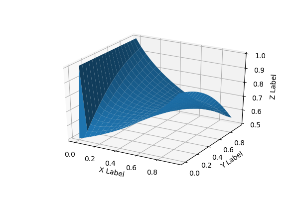
Figure 1: Surface Plot of SBAF

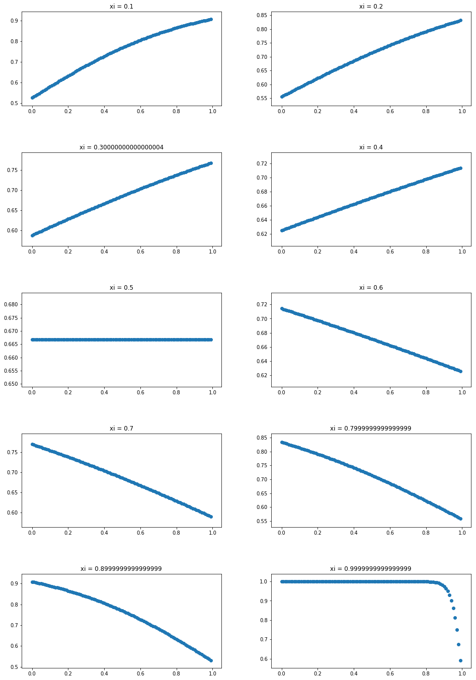
Figure 2:

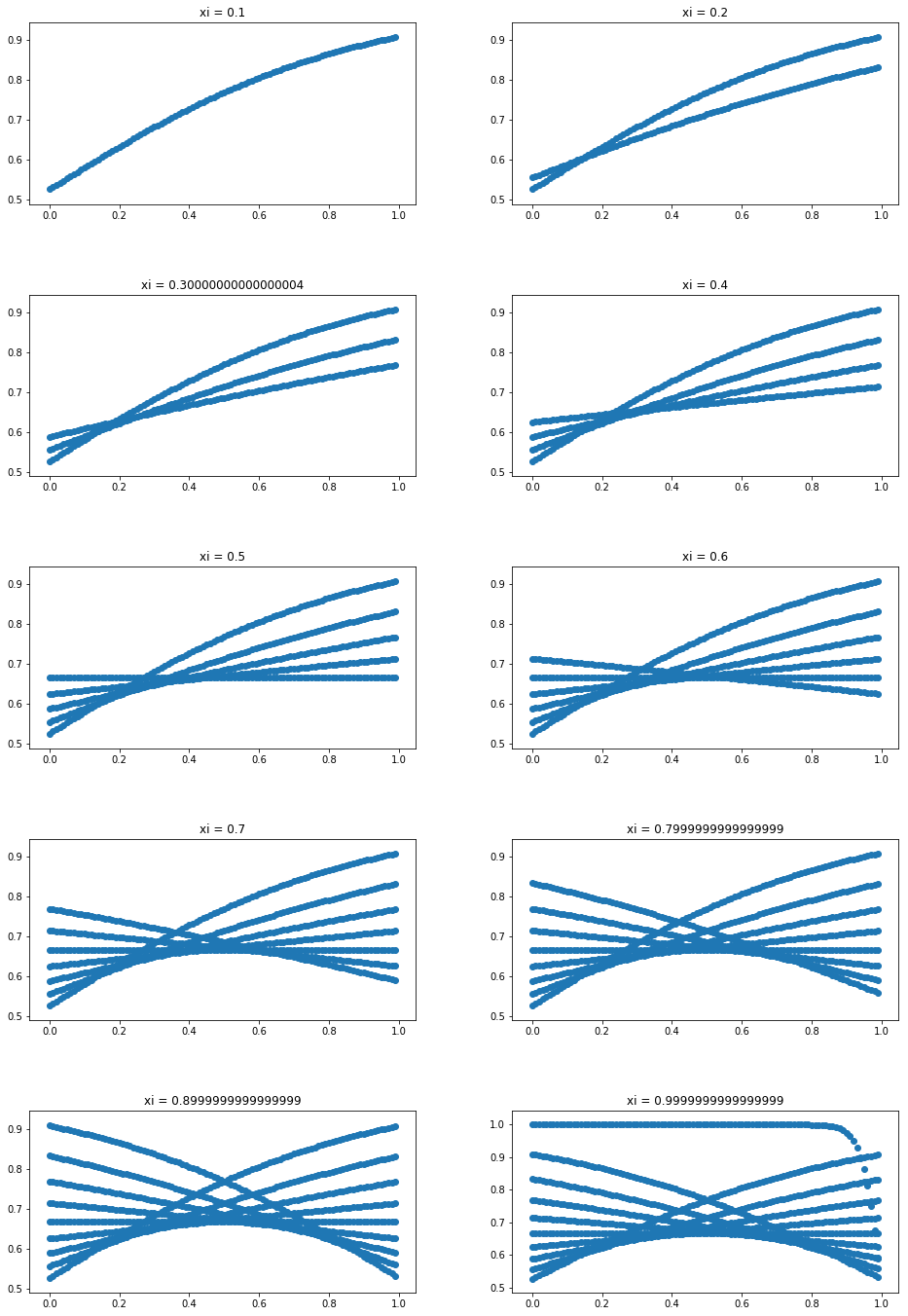
Figure 3:

2.1 Existence of Optima: Second order Differentiation of SBAF for Neural Network

From Equation 3 ,

$$\begin{split}\frac{dy}{dx}&=\frac{y(1-y)}{x(1-x)}\cdot(\alpha-x)\end{split}$$

Therefore,

$$\begin{split}\frac{d^{2}y}{dx^{2}}&=\frac{x(1-x)\frac{d[y(1-y)\cdot(\alpha-x)]}{dx}-[y(1-y)\cdot(\alpha-x)]\frac{d(x(1-x))}{dx}}{(x(1-x))^{2}}\\ &=\frac{x(1-x)\frac{d[(y-y^{2})\cdot(\alpha-x)]}{dx}-[(y-y^{2})\cdot(\alpha-x)]\frac{d(x-x^{2})}{dx}}{(x(1-x))^{2}}\\ &=\frac{x(1-x)[(\alpha-x)\frac{d(y-y^{2})}{dx}+(y-y^{2})\cdot\frac{d(\alpha-x)}{dx}]-[(y-y^{2})\cdot(\alpha-x)]\cdot(1-2x)}{(x(1-x))^{2}}\\ &=\frac{x(1-x)[(\alpha-x)\cdot(\frac{dy}{dx}-2y\frac{dy}{dx})+(y-y^{2})(-1)]-[(y-y^{2})\cdot(\alpha-x)]\cdot(1-2x)}{(x(1-x))^{2}}\\ \end{split}$$

$$\begin{split}\Rightarrow\frac{d^{2}y}{dx^{2}}&=\frac{x(1-x)[(\alpha-x)\cdot(1-2y)\cdot\frac{dy}{dx}+y(y-1)]+y(y-1)\cdot(\alpha-x)\cdot(1-2x)}{(x(1-x))^{2}}\\ \end{split}$$ (4)

Now, substituting 1 in 4 we get,

$$\begin{split}\Rightarrow\frac{d^{2}y}{dx^{2}}&=\frac{x(1-x)(\alpha-x)\cdot(1-2y)\cdot\Big{[}\frac{y(1-y)}{x(1-x)}\cdot(\alpha-x)\Big{]}+x(1-x)\cdot y(y-1)+y(y-1)\cdot(\alpha-x)\cdot(1-2x)}{(x(1-x))^{2}}\\ &=\frac{y(y-1)[x(1-x)+(\alpha-x)\cdot(1-2x)+(\alpha-x)^{2}\cdot(1-2y)]}{(x(1-x))^{2}}\\ \end{split}$$

when $\alpha=x$,

$$\begin{split}\Rightarrow\frac{d^{2}y}{dx^{2}}&=\frac{x(1-x)\cdot y(y-1)}{(x(1-x))^{2}}\\ &=\frac{y(y-1)}{x(1-x)}\\ \end{split}$$

Clearly, the first derivative vanishes when $\alpha=x$, the derivative is positive when $\alpha>x$ and is negative when $\alpha<x$ (implying range of values for $\alpha$ so that the function becomes increasing or decreasing, please see Eq. (3)). We need to determine the sign of the second derivative when $\alpha=x$ to ascertain the condition of maxima (corresponding to maximum width of the separating hyperplane ensuring optimal discrimination between habitability classes). Assuming $0<x<1$, the condition of optimality, $0\leq\alpha\leq 1$, $y$ by construction lies between $(0,1)$. Hence, $\frac{d^{2}y}{dx^{2}}<0$ ensuring maxima of $y$.

3 Backpropagation with SBAF

The basic structure of the neural network consists of input layer, hidden layer and output layer. Let us assume the nodes at input layer are $i_{1}$, $i_{2}$ , at hidden layer $h_{1}$, $h_{2}$ and at output layer $o_{1}$, $o_{2}$.

3.1 Basic Structure

Goal: to optimize the weights so that the network can learn how to map from inputs to outputs.

3.2 The Forward Pass

Calculate the total input for $h_{1}$.

$$h1_{net}=w_{1}\cdot i_{1}+w_{2}\cdot i_{2}+b_{1}$$

$$h2_{net}=w_{3}\cdot i_{1}+w_{4}\cdot i_{2}+b_{1}$$

Use SBAF to calculate the output for $h_{1}$, $y=\frac{1}{1+kx^{\alpha}(1-x)^{1-\alpha}}$.

$$h1_{out}=\frac{1}{1+k(h1_{net})^{\alpha}(1-h1_{net})^{1-\alpha}}$$

$$h2_{out}=\frac{1}{1+k(h2_{net})^{\alpha}(1-h2_{net})^{1-\alpha}}$$

Repeat the process for output layer neuron.

$$o1_{net}=w_{5}\cdot h1_{out}+w_{6}\cdot h2_{out}+b_{2}$$

$$o2_{net}=w_{7}\cdot h1_{out}+w_{8}\cdot h2_{out}+b_{2}$$

The outputs are

$$o1_{out}=\frac{1}{1+k(o1_{net})^{\alpha}(1-o1_{net})^{1-\alpha}}$$

$$o2_{out}=\frac{1}{1+k(o2_{net})^{\alpha}(1-o2_{net})^{1-\alpha}}$$

Calculating the errors,

$$\mathrm{Error}=\mathrm{Error}_{o1}+\mathrm{Error}_{o2}$$

$$\mathrm{Error}_{o1}=\frac{1}{2}\left(o1_{target}-o1_{out}\right)^{2}$$

$$\mathrm{Error}_{o2}=\frac{1}{2}\left(o2_{target}-o2_{out}\right)^{2}$$

3.3 The Backward Pass

Update the weights so that the actual output is closer to target output, thereby minimizing the error.

3.3.1 Output Layer

Consider $w_{5}$: let’s find the gradient wrt $w_{5}$, i.e., $\frac{\partial E_{total}}{\partial w_{5}}$.

$$\boxed{\frac{\partial E_{T}}{\partial w_{5}}=\frac{\partial E_{T}}{\partial o1_{out}}\cdot\frac{\partial o1_{out}}{\partial o1_{net}}\cdot\frac{\partial o1_{net}}{\partial w_{5}}}$$

Calculate each component on the RHS one by one:

$$\boxed{\begin{aligned} \partial E_{T}&=E_{o1}+E_{o2}\\ E_{T}&=\frac{1}{2}\left(o1_{target}-o1_{out}\right)^{2}+\frac{1}{2}\left(o2_{target}-o2_{out}\right)^{2}\\ \frac{\partial E}{\partial o1_{out}}&=2\cdot\frac{1}{2}\left(o1_{target}-o1_{out}\right)\cdot(-1)+0\\ \frac{\partial E}{\partial o1_{out}}&=-\left(o1_{target}-o1_{out}\right)\end{aligned}}\qquad$$ (5)

Using the SBAF

$$\boxed{\begin{aligned} o1_{out}&=\frac{1}{1+k(o1_{net})^{\alpha}(1-o1_{net})^{1-\alpha}}\\ \frac{\partial o1_{out}}{\partial o1_{net}}&=\frac{o1_{out}(1-o1_{out})}{o1_{net}(1-o1_{net})}\cdot(\alpha-o1_{net})\end{aligned}}\qquad$$ (6)

Finally,

$$\boxed{\begin{aligned} o1_{net}&=w_{5}\cdot h1_{out}+w_{6}\cdot h2_{out}+b_{2}\\ \frac{\partial o1_{net}}{\partial w_{5}}&=h1_{out}\end{aligned}}\qquad$$ (7)

Putting $(1)$ and $(2)$ and $(3)$ together in $\frac{\partial E_{T}}{\partial w_{5}}$,

$$\frac{\partial E_{T}}{\partial w_{5}}=-\left(o1_{target}-o1_{out}\right)\cdot\frac{o1_{out}(1-o1_{out})}{o1_{net}(1-o1_{net})}\cdot(\alpha-o1_{net})\cdot h1_{out}$$

$$w_{5}^{new}=w_{5}-\eta\cdot\frac{\partial E_{T}}{\partial w_{5}}$$ (8)

where $\eta$ is the learning rate.
Likewise,

$$\frac{\partial E_{T}}{\partial w_{6}}=-\left(o1_{target}-o1_{out}\right)\cdot\frac{o1_{out}(1-o1_{out})}{o1_{net}(1-o1_{net})}\cdot(\alpha-o1_{net})\cdot h2_{out}\\$$

$$\frac{\partial E_{T}}{\partial w_{7}}=-\left(o2_{target}-o2_{out}\right)\cdot\frac{o2_{out}(1-o2_{out})}{o2_{net}(1-o2_{net})}\cdot(\alpha-o2_{net})\cdot h1_{out}$$

$$\frac{\partial E_{T}}{\partial w_{8}}=-\left(o2_{target}-o2_{out}\right)\cdot\frac{o2_{out}(1-o2_{out})}{o2_{net}(1-o2_{net})}\cdot(\alpha-o2_{net})\cdot h2_{out}$$

3.3.2 Hidden Layer

Consider $w_{1}$

We need to find $\frac{\partial E_{T}}{\partial w_{1}}$.
Apparently,

$$\frac{\partial E_{T}}{\partial w_{1}}=\frac{\partial E_{o1}}{\partial w_{1}}+\frac{\partial E_{o2}}{\partial w_{1}}$$

The chain rule says,

$$\frac{\partial E_{o1}}{\partial w_{1}}=\frac{\partial E_{o1}}{\partial o1_{out}}\cdot\frac{\partial o1_{out}}{\partial o1_{net}}\cdot\frac{\partial o1_{net}}{\partial h1_{out}}\cdot\frac{\partial h1_{out}}{\partial h1_{net}}\cdot\frac{\partial h1_{net}}{\partial w_{1}}$$ (1)

$$\frac{\partial E_{o2}}{\partial w_{1}}=\frac{\partial E_{o2}}{\partial o2_{out}}\cdot\frac{\partial o2_{out}}{\partial o2_{net}}\cdot\frac{\partial o2_{net}}{\partial h1_{out}}\cdot\frac{\partial h1_{out}}{\partial h1_{net}}\cdot\frac{\partial h1_{net}}{\partial w_{1}}$$ (2)

Computing all the components of equation $(1)$,

$$\frac{\partial E_{o1}}{\partial o1_{out}} =-(o1_{target}-o1_{out})$$

$$\frac{\partial o1_{out}}{\partial o1_{net}} =\frac{o1_{out}(1-o1_{out})}{o1_{net}(1-o1_{net})}\cdot(\alpha-o1_{net})$$

$$\frac{\partial o1_{net}}{\partial h1_{out}} =w_{5}\left(\because o1_{net}=w_{5}\cdot h1_{out}+w_{6}\cdot h2_{out}+b_{2}\text{ and }\frac{\partial o1_{net}}{\partial h1_{out}}=w_{5}\right)$$

$$\frac{\partial h1_{out}}{\partial h1_{net}} =\frac{h1_{out}(1-h1_{out})}{h1_{net}(1-h1_{net})}\cdot(\alpha-h1_{net})$$

$$\frac{\partial h1_{net}}{\partial w_{1}} =i_{1}\left(\because h1_{net}=w_{1}i_{1}+w_{2}i_{2}+b_{1}\text{ and }\frac{\partial h1_{net}}{\partial w_{1}}=i_{1}+0\right)$$

Similarly, computing all the components of $(2)$,

$$\frac{\partial E_{o2}}{\partial o2_{out}} =-(o2_{target}-o2_{out})$$

$$\frac{\partial o2_{out}}{\partial o2_{net}} =\frac{o2_{out}(1-o2_{out})}{o2_{net}(1-o2_{net})}\cdot(\alpha-o2_{net})$$

$$\frac{\partial o2_{net}}{\partial h1_{out}} =w_{7}\left(\because o2_{net}=w_{7}h1_{out}+w_{8}h2_{out}+b2\right)$$

We know $\frac{\partial h1_{out}}{\partial h1_{net}}$ and $\frac{\partial h1_{net}}{\partial w_{1}}$.

Adding up everything,

$$\frac{\partial E_{T}}{\partial w_{1}}=\frac{\partial E_{o1}}{\partial w_{1}}+\frac{\partial E_{o2}}{\partial w_{2}}$$

$$\boxed{w_{1}=w_{1}-\eta\cdot\frac{\partial E_{T}}{\partial w_{1}}}\qquad$$

Likewise, $\frac{\partial E_{T}}{\partial w_{2}}$, $\frac{\partial E_{T}}{\partial w_{2}}$, $\frac{\partial E_{T}}{\partial w_{3}}$, and $\frac{\partial E_{T}}{\partial w_{4}}$ can be computed.

4 Discussion

• $x$ is surface temperature (normalized between $0$ and $1$) and $1-x$ is the complement of that, together explaining the perfect discrimination between habitability classes as explained in our TSS above. The motivation of SBAF is derived from this fact of TSS. Using $kx^{\alpha}(1-x)^{1-\alpha}$ shall maximize the width of the two separating hyperplanes in the SVM used in TSS (See the proof below) as the kernel has a global maxima when $0\leq\alpha\leq 1$. This is equivalent to the CDHS formulation when CD-HPF is written as $y=kx^{\alpha}(1-x)^{\beta}$ where $\alpha+\beta=1,0\leq\alpha\leq 1,0\leq\beta\leq 1$, $k$ is suitably assumed to be $1$ (CRS condition), and the representation ensures global maxima (maximum width of the separating hyperplanes) under such constraints [Bora et al., 2016, Saha et al., 2017].

• The new activation function to be used for training a neural network for habitability classification boasts of an optima. Evidently, from the graphical simulations below, we observe less flattening of the function and therefore the formulation should be able to tackle local oscillations more easily as compared to the more generally used sigmoid function. Moreover, since $0\leq\alpha\leq 1,0\leq x\leq 1,0\leq 1-x\leq 1$, the variable term in the denominator of SBAF, $kx^{\alpha}(1-x)^{1-\alpha}$ may be approximated to a first order polynomial. This may help us in circumventing expensive floating point operations without compromising the precision.

• Need to show that the maxima is unique in the defined interval. This will circumvent the local maxima problem.

Habitability classification is a complex task. Even though the literature is replete with rich and sophisticated methods using both supervised [Zighed et al., 2010] and unsupervised learning methods, the soft margin between classes, namely psychroplanet and mesoplanet makes the task of discrimination incredibly difficult. A sequence of recent explorations by Saha et. al. expanding previous work by Bora et. al. on using Machine Learning algorithm to construct and test planetary habitability functions with exoplanet data raises important questions. The 2018 paper ([Saha et al., 2017]) analyzed the elasticity of the Cobb-Douglas Habitability Score (CDHS) and compared its performance with other machine learning algorithms. They demonstrated the robustness of their methods to identify potentially habitable planets [Saha et al., 2018b] from exoplanet dataset. Given our little knowledge on exoplanets and habitability, these results and methods provide one important step toward automatically identifying objects of interest from large datasets by future ground and space observatories. The variable term in SBAF, $kx^{\alpha}(1-x)^{1-\alpha}$ is inspired from a history of modeling such terms as production functions and exploiting optimization principles in production economics, [Saha et al., 2016], [Ginde et al., 2016], [Ginde et al., 2015]. Complexities/bias in data may often necessitate devising classification methods to mitigate class imbalance, [Mohanchandra et al., 2015] to improve upon the original method, [Vapnik and Chervonenkis, 1964], [Cortes and Vapnik, 1995] or manipulate confidence intervals [Khaidem et al., 2016]. However, these improvisations led the authors to believe that, a general framework to train in forward and backward pass may turn out to be efficient. This is the primary reason to design a neural network with a novel activation function. We shall use the architecture to discriminate exoplanetary habitability [Schulze-Makuch and Bains, 2018], [Schulze-Makuch et al., 2011], [Irwin et al., 2014], [Shallue and Vanderburg, 2018], [Méndez, 2011], [Méndez, 2018].

References

References

- Agrawal et al. [2018] Agrawal, S., Basak, S., Saha, S., Bora, K., Murthy, J., 2018. A comparative analysis of the cobb-douglas habitability score (cdhs) with the earth similarity index (esi). arXiv:arXiv:1804.11176.
- Bains and Schulze-Makuch [2016] Bains, W., Schulze-Makuch, D., 2016. The cosmic zoo: The (near) inevitability of the evolution of complex, macroscopic life. Life 6, 25. URL: https://doi.org/10.3390/life6030025, doi:10.3390/life6030025.
- Basak et al. [2018] Basak, S., Agrawal, S., Saha, S., Theophilus, A.J., Bora, K., Deshpande, G., Murthy, J., 2018. Saha-bora activation function: Habitability classification. arXiv:10.13140/RG.2.2.21081.62565.
- Bora et al. [2016] Bora, K., Saha, S., Agrawal, S., Safonova, M., Routh, S., Narasimhamurthy, A., 2016. Cd-hpf: New habitability score via data analytic modeling. Astronomy and Computing 17, 129 -- 143. URL: http://www.sciencedirect.com/science/article/pii/S2213133716300865, doi:https://doi.org/10.1016/j.ascom.2016.08.001.
- Cortes and Vapnik [1995] Cortes, C., Vapnik, V., 1995. Support-vector networks. Machine Learning 20, 273--297. URL: https://doi.org/10.1023/A:1022627411411, doi:10.1023/A:1022627411411.
- Elfwing et al. [2018] Elfwing, S., Uchibe, E., Doya, K., 2018. Sigmoid-weighted linear units for neural network function approximation in reinforcement learning. Neural Networks URL: http://www.sciencedirect.com/science/article/pii/S0893608017302976, doi:https://doi.org/10.1016/j.neunet.2017.12.012.
- Ginde et al. [2015] Ginde, G., Saha, S., Balasubramaniam, C., Harsha, R., Mathur, A., Dayasagar, B., Anand, M., 2015. Mining massive databases for computation of scholastic indices: Model and quantify internationality and influence diffusion of peer-reviewed journals, in: Proceedings of the fourth national conference of Institute of Scientometrics, SIoT.
- Ginde et al. [2016] Ginde, G., Saha, S., Mathur, A., Venkatagiri, S., Vadakkepat, S., Narasimhamurthy, A., Daya Sagar, B.S., 2016. Scientobase: a framework and model for computing scholastic indicators of non-local influence of journals via native data acquisition algorithms. Scientometrics 108, 1479--1529. URL: https://doi.org/10.1007/s11192-016-2006-2, doi:10.1007/s11192-016-2006-2.
- Irwin et al. [2014] Irwin, L., Méndez, A., Fairén, A., Schulze-Makuch, D., 2014. Assessing the possibility of biological complexity on other worlds, with an estimate of the occurrence of complex life in the milky way galaxy. Challenges 5, 159--174. URL: https://doi.org/10.3390/challe5010159, doi:10.3390/challe5010159.
- Khaidem et al. [2016] Khaidem, L., Saha, S., Basak, S., Dey, S.R., 2016. Predicting the direction of stock market prices using random forest. URL: "https://www.researchgate.net/publication/301818771_Predicting_the_direction_of_stock_market_prices_using_random_forest".
- Lippmann [1994] Lippmann, R., 1994. Book review: "neural networks, a comprehensive foundation", by simon haykin. International Journal of Neural Systems 05, 363--364. URL: https://doi.org/10.1142/s0129065794000372, doi:10.1142/s0129065794000372.
- Méndez [2011] Méndez, A., 2011. The night sky of exoplanets URL: http://phl.upr.edu/library/notes/syntheticstars.
- Méndez [2018] Méndez, A., 2018. The habitable exoplanets catalog URL: http://phl.upr.edu/hec.
- Mohanchandra et al. [2015] Mohanchandra, K., Saha, S., Murthy, K.S., Lingaraju, G., 2015. Distinct adoption of k-nearest neighbour and support vector machine in classifying EEG signals of mental tasks. International Journal of Intelligent Engineering Informatics 3, 313. URL: https://doi.org/10.1504/ijiei.2015.073064, doi:10.1504/ijiei.2015.073064.
- Saha et al. [2017] Saha, S., Basak, S., Bora, K., Safonova, M., Agrawal, S., Sarkar, P., Murthy, J., 2017. Theoretical Validation of Potential Habitability via Analytical and Boosted Tree Methods: An Optimistic Study on Recently Discovered Exoplanets. ArXiv e-prints arXiv:1712.01040.
- Saha et al. [2018a] Saha, S., Bora, K., Basak, S., Mathur, A., Agrawal, S., 2018a. Habitability classification of exoplanets: A machine learning insight. arXiv:arXiv:1805.08810.
- Saha et al. [2018b] Saha, S., Bora, K., Basak, S., Srinivasa, G., Safonova, M., Murthy, J., Agrawal, S., 2018b. Ebook-astroinformatics series machine learning in astronomy: A workman’s manual. URL: "https://www.researchgate.net/publication/322926268_EBOOK-ASTROINFORMATICS_SERIES_MACHINE_LEARNING_IN_ASTRONOMY_A_WORKMAN’S_MANUAL".
- Saha et al. [2016] Saha, S., Sarkar, J., Dwivedi, A., Dwivedi, N., Narasimhamurthy, A.M., Roy, R., 2016. A novel revenue optimization model to address the operation and maintenance cost of a data center. Journal of Cloud Computing 5, 1. URL: https://doi.org/10.1186/s13677-015-0050-8, doi:10.1186/s13677-015-0050-8.
- Saha et al. [2018c] Saha, S., Sarkar, P., Mathur, A., Basak, S., 2018c. Model visualization in understanding rapid growth of a journal in an emerging area. arXiv:arXiv:1803.04644.
- Schulze-Makuch and Bains [2018] Schulze-Makuch, D., Bains, W., 2018. Time to consider search strategies for complex life on exoplanets. Nature Astronomy , 1--2URL: http:https://doi.org/10.1038/s41550-018-0476-2, doi:10.1038/s41550-018-0476-2.
- Schulze-Makuch et al. [2011] Schulze-Makuch, D., Méndez, A., Fairén, A.G., von Paris, P., Turse, C., Boyer, G., Davila, A.F., de Sousa António, M.R., Catling, D., Irwin, L.N., 2011. A two-tiered approach to assessing the habitability of exoplanets. Astrobiology 11, 1041--1052. URL: https://doi.org/10.1089/ast.2010.0592, doi:10.1089/ast.2010.0592.
- Shallue and Vanderburg [2018] Shallue, C.J., Vanderburg, A., 2018. Identifying exoplanets with deep learning: A five-planet resonant chain around kepler-80 and an eighth planet around kepler-90. The Astronomical Journal 155, 94. URL: http://stacks.iop.org/1538-3881/155/i=2/a=94.
- Vapnik and Chervonenkis [1964] Vapnik, V.N., Chervonenkis, A.Y., 1964. On a class of perceptrons. Automation and Remote Control 1, 103--109.
- [24] Younger, A., Hochreiter, S., Conwell, P., . Meta-learning with backpropagation, in: IJCNN 01. International Joint Conference on Neural Networks. Proceedings (Cat. No.01CH37222), IEEE. URL: https://doi.org/10.1109/ijcnn.2001.938471, doi:10.1109/ijcnn.2001.938471.
- Zighed et al. [2010] Zighed, D.A., Ritschard, G., Marcellin, S., 2010. Asymmetric and Sample Size Sensitive Entropy Measures for Supervised Learning. Springer Berlin Heidelberg, Berlin, Heidelberg. pp. 27--42. URL: https://doi.org/10.1007/978-3-642-05183-8_2, doi:10.1007/978-3-642-05183-8_2.