The Effect of Planning Shape on Dyna-style Planning
in High-dimensional State Spaces

Abstract

Dyna is a fundamental approach to model-based reinforcement learning (MBRL) that interleaves planning, acting, and learning in an online setting. In the most typical application of Dyna, the dynamics model is used to generate one-step transitions from selected start states from the agent’s history, which are used to update the agent’s value function or policy as if they were real experiences. In this work, one-step Dyna was applied to several games from the Arcade Learning Environment (ALE). We found that the model-based updates offered surprisingly little benefit over simply performing more updates with the agent’s existing experience, even when using a perfect model. We hypothesize that to get the most from planning, the model must be used to generate unfamiliar experience. To test this, we experimented with the “shape” of planning in multiple different concrete instantiations of Dyna, performing fewer, longer rollouts, rather than many short rollouts. We found that planning shape has a profound impact on the efficacy of Dyna for both perfect and learned models. In addition to these findings regarding Dyna in general, our results represent, to our knowledge, the first time that a learned dynamics model has been successfully used for planning in the ALE, suggesting that Dyna may be a viable approach to MBRL in the ALE and other high-dimensional problems.

1 Introduction

Dyna Sutton (1990) is a general architecture for reinforcement learning (RL) agents that flexibly combines aspects of both model-free and model-based RL. In Dyna, the agent learns a predictive model of its environment, which is used to generate simulated experience alongside the agent’s real experience. Both types of experience are used in the same way: to update the agent’s value function and/or policy. Planning in this way is referred to as Dyna-style planning.

Dyna-style planning has many appealing properties that make it a potentially powerful approach in large-scale problems. Because the model indirectly influences the agent’s behavior via the value function or policy, the computationally expensive process of planning can be asynchronous with the agent’s decision-making loop, retaining a model-free agent’s ability to operate on a fine-grained timescale. Furthermore, Dyna permits flexible control over how much computational effort is devoted to planning and how that planning effort is distributed, potentially focusing on updates that will have the most impact, as in Prioritized Sweeping Moore and Atkeson (1993). That said, there have been relatively few examples of the application of Dyna-style planning in large-scale problems with high-dimensional observations, such as images.

In this work we study the behavior of Dyna in the Arcade Learning Environment (ALE) Bellemare et al. (2013a), where agents learn to play games from the Atari 2600 system with raw images as input. Though many successful methods exist for playing games from the ALE and other image based domains (e.g. Mnih et al. (2015, 2016); Hessel et al. (2018)), the majority of these approaches can be considered model-free, in that they learn and improve a policy without using a predictive model of the environment. Model-based methods have the potential to offer dramatic sample complexity benefits and are thus of significant interest. However, despite the introduction of increasingly effective approaches for learning predictive models in Atari games Bellemare et al. (2013b, 2014); Oh et al. (2015a), the application of model-based methods to the ALE is still an open problem, with many challenges to overcome Machado et al. (2017).

Though some recent approaches to image-based problems incorporate model-like components (e.g. Tamar et al. (2016); Oh et al. (2017); Weber et al. (2017)), these methods arguably discard many of the anticipated benefits of model-learning by making the model essentially a part of the parameterization of the value function or policy. Part of the allure of model-based RL is that a dynamics model could be learned even when the agent has little guidance on how to behave and that the model can be used as a substitute for gathering expensive experience in the real world. In this work we focus on learning and directly planning with a dynamics model.

In the original Dyna-Q algorithm Sutton (1990), planning was performed by selecting several states from the agent’s recent experience and using the model to roll forward one step from each of those states and thus generate value function updates. This remains the most common form of Dyna-style planning. In our experiments in the ALE we found that using the model in this way provided surprisingly little benefit, even with a perfect model — similar sample efficiency gains could be obtained simply by performing more model-free updates on the data the agent had already gathered. We note, however, that Dyna-style planning can take on a variety of shapes. For a fixed budget of model interactions, one might generate many one-step rollouts or fewer multi-step rollouts. Empirically we find that planning with longer rollouts yields dramatic improvement when using a perfect model. We also find that planning shape impacts performance when the model is learned (and is therefore imperfect), though model flaws can make rollouts unreliable.

The primary contribution of this paper is an empirical exploration of the impact of planning shape on Dyna-style planning. The results offer guidance to future practitioners wishing to apply Dyna. In particular, we find that:

1. For Dyna to take full advantage of a model, it must use the model to generate unfamiliar experience (in essence to replace exploration in the real environment).

2. Performing longer rollouts in the model seems to be a simple, effective way to generate unfamiliar experience.

3. Planning shape seems to be an important consideration even when the model is imperfect.

4. Even if there were dramatic improvements in model-learning, where highly accurate models could be learned very quickly, there would still be little benefit from planning with one-step rollouts. Longer rollouts are necessary to allow planning to exploit more accurate models.

Furthermore, though this paper is primarily focused on the above scientific observations and not on generating new state of the art results in the ALE, the experimental results demonstrate for the first time (as far as we are aware) a sample-complexity benefit from learning a dynamics model in some games. This benefit is at its greatest with proper choice of planning shape. Model-based reinforcement learning in the ALE has proven to be such a challenge that even a modest benefit from a learned model is a significant and unprecedented development Machado et al. (2017). This finding may point the way toward yet more effective model-based approaches in this domain and establishes Dyna as a viable planning method in large-scale, high-dimensional domains.

2 The Ineffectiveness of One-step Rollouts

Planning in the Dyna architecture is accomplished by using a model to make predictions of future states based on a start state and action. When the state is high dimensional, like an image, it is not clear how to generate reasonable start states. One solution is to sample the start state from the previously observed states, as in Dyna-Q Sutton (1990). The advantage of selecting states in this way is that the distribution or structure of the state space does not need to be known, but planning may not be guaranteed to cover the state space entirely. To explore this strategy we experiment with Dyna in several Atari games.

Dyna is a meta-algorithm. To instantiate it, one must make specific choices for the model and the value function/policy learner. In the experiments in this section, the agent uses a perfect model. This allows us to investigate best case planning performance and focus on the question of how best to use the model. In Sections 4 and 5 we incorporate imperfect, learned models.

We experimented with agents based on two different value function learners. One was based on the Sarsa algorithm Rummery and Niranjan (1994); Sutton (1996), using linear value function approximation with Blob-PROST features Liang et al. (2016), which have been shown to perform well in the ALE. The other was based on Deep Q-Networks (DQN) Mnih et al. (2015), which approximates the value function using a deep convolutional neural network. Qualitatively, the results were very similar for both agents, suggesting that our conclusions are robust to different concrete instantiations of the Dyna architecture. Here we focus on the results from the DQN-based agent; the results from the Sarsa-based agent can be found in the appendix.

2.1 Deep Q-networks and Dyna-DQN

Deep Q-networks (DQN) Mnih et al. (2015) is a model-free RL method, based on Q-learning, that uses a deep convolutional neural network to approximate the value function. Unlike Q-learning, DQN does not update the value function after every step using a single transition; instead, DQN uses experience replay Lin (1992), and places each observed transition into an experience replay buffer. Then, for a single training step, the algorithm selects a batch of transitions from the buffer uniformly at random to update the parameters. Training steps are performed after every $f$ observed transitions, which is referred to as the training frequency.

It is straightforward to extend DQN to incorporate it into the Dyna architecture. Our approach, which we call Dyna-DQN, is similar to other recent attempts to combine DQN with planning (e.g. Gu et al. (2016); Kalweit and Boedecker (2017); Peng et al. (2018)). After every step taken in the environment, a number of start states for planning are sampled from a planning buffer containing the agent’s recent real experience. Keeping a separate buffer ensures that start states are always from the agent’s actual experience. For each start state, an action is selected using the agent’s current policy and the model is used to simulate a single transition, which is placed into the experience replay buffer alongside the transitions observed from the real environment. Training continues to happen after every $f$ observed transitions — real or simulated. As a result, batches sampled at training time will contain a mix of real and simulated experience.

2.2 Experiments

We ran experiments on six games from the ALE and used sticky actions to inject stocasticity into the emulator (repeat_action_probability = 0.25), as suggested by Machado et al. Machado et al. (2017). Each game usually has 18 possible actions, but some actions are redundant in certain games. Therefore, we used the minimal action set like Mnih et al. Mnih et al. (2015).

We chose to study the games from the original training set outlined by Bellemare et al. Bellemare et al. (2013a), supplemented with two additional games, Q-Bert and Ms. Pac-Man, that Oh et al. Oh et al. (2015a) used to evaluate their model learning approach, which we employ later. We have omitted results in Freeway since our implementations of DQN and Dyna-DQN almost always score zero points at the number of training frames we used.

Our implementation of DQN used the same hyper-parameters as Mnih et al. Mnih et al. (2015) with a few small changes used by Machado et al. Machado et al. (2017). At each step, DQN has an $\epsilon$ probability of selecting a random action instead of the best action. We annealed $\epsilon$ from 1.0 to 0.01 over the first 10% of frames (real and simulated) during learning. The frame skip is the number of times a selected action is repeated before a new action is selected. We used a frame skip of 5. Additionally, to reduce memory use, we used an experience replay buffer size of 500k transitions instead of the original 1M.

As described above, in these experiments, the agent used a perfect copy of the emulator for its model. Start states for planning were selected from the planning buffer containing the 10,000 most recent real states observed by the agent, which for all games was multiple episodes of experience. For each real step, Dyna-DQN drew 100 start states from the buffer and simulated a single transition from each. Dyna-DQN was trained for 100k real frames, or equivalently 10M combined model and real frames. The training frequency was every 4 steps of real and model experience. After training, the mean score in 100 evaluation episodes using a fixed $\epsilon=0.01$ was recorded. This training and evaluation procedure was repeated for thirty independent runs. The mean scores and standard errors for the six games are shown in Figure 1. The bright green bars labeled $100\times 1$ represent Dyna-DQN; the dark green bars will be described in Section 3.

To better evaluate the benefit of model-based updates, we also compared to the following model-free DQN baselines (pictured as horizontal lines in Figure 1).

DQN 100k: DQN trained only for 100k real frames (yellow lines). This allows us to compare DQN and Dyna-DQN with an equivalent amount of real experience. This benchmark serves as a sanity check to show that using the perfect model to gather additional data does improve sample complexity. As expected, Dyna-DQN outperformed DQN 100k; it uses the model to generate more experience and does many more updates. However, this benchmark does not indicate whether the performance increase is due to the additional data generated by Dyna-DQN, or the extra updates to the value function completed during planning.

DQN Extra Updates: DQN trained for 100k real frames, but with the same number of updates to the value function as Dyna-DQN (red lines). For each time DQN would normally perform a single training step, DQN Extra Updates performs 100 training steps. This way DQN Extra Updates is like Dyna-DQN, but it uses only experience gathered from the environment, while Dyna-DQN also generates experience from the model. DQN Extra Updates allows us to isolate the advantage of using the model to generate new experience compared to simply doing more updates with the real experience. Surprisingly, in every game excluding Seaquest, Dyna-DQN provided little benefit over DQN Extra Updates, even with a perfect model. This indicates that most of the benefit of planning was from simply updating the value function more often, which does not require a model.

DQN 10M: DQN trained for 10M frames (cyan lines). This allows us to compare DQN and Dyna-DQN with an equivalent amount of total experience. We might hope the experience generated by a perfect model would allow Dyna-DQN to perform comparably to this baseline, but in most games the performance of Dyna-DQN did not approach that of DQN 10M. This shows that there is significant room to improve the performance. Dyna-DQN and DQN 10M both gather additional data from the true system and perform the same number of updates; the only difference is the distribution over the start states of the additional transitions.

Overall, we find that the extra computation required by Dyna to utilize the model does not appear to be worth the effort. Here we re-emphasize that this finding is robust to different choices for value function learners within the Dyna architecture; we obtained similar results using an agent based on Sarsa with linear value function approximation rather than DQN (see the online appendix). It seems that planning in this way — taking a single step from a previously visited state — does not provide data that is much different than what is already contained in the experience replay buffer. If true, a strategy is needed to make the data generated by the model different from what was already experienced.

(a)

(b)

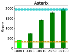
(c)

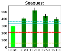
(d)

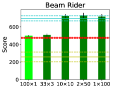
(e)

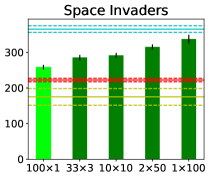
(f)

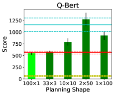
(g)

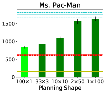
(h)

Figure 1: The results of running Rollout-Dyna-DQN on six games from the ALE compared to DQN baselines. The bright green bars represent Dyna-DQN (Section 2.2). The dark green bars represent Rollout-Dyna-DQN with various planning shapes (Section 3.1). The horizontal lines show the baseline scores (see Section 2.2).

3 Planning with Longer Rollouts

We hypothesize that it may be possible to generate more diverse experience by rolling out more than a single step from the start state during planning. Since the current policy will be used for the rollout, the model may generate a different trajectory than what was originally observed. Longer rollouts would also allow the agent to see the longer-term consequences of exploratory actions or alternative stochastic outcomes. In existing work longer rollouts have been employed in Dyna-style planning (e.g. Gu et al. (2016); Kalweit and Boedecker (2017)), but the impact of this choice has not been extensively or systematically studied.

It is straightforward to modify Dyna-DQN so that instead of rolling out a single step, the model is used to roll out $k$ steps from each start state, producing a sequence of $k$ states and rewards, which are all placed in the experience replay buffer. Let this algorithm be called Rollout-Dyna-DQN. When $k=1$ we recover exactly Dyna-DQN.

Given a budget of planning time in terms of a fixed number of model prediction steps, planning could take on a variety of shapes. Let the planning shape be described by the notation $n$$\times$$k$, where $n$ is the number of start states. For example: 100 rollouts of 1 step (100$\times$1); 10 rollouts of 10 steps (10$\times$10); or 1 rollout of 100 steps (1$\times$100), each require the same amount of computation from the model. The experience generated during a multi-step rollout is still recorded as single transitions in the replay buffer, to be sampled independently during a DQN training step. Furthermore we hold the total number of transitions drawn from the model constant. Thus the only difference between two planning shapes is the distribution of transitions in the replay buffer. In the next section we investigate the effects of planning shape on the performance of Dyna-style planning.

3.1 Experiments

Our experimental setup is the same as in the Section 2.2, but now the planning shape for Dyna-DQN is varied. We trained and evaluated 100$\times$1, 33$\times$3, 10$\times$10, 2$\times$50, and 1$\times$100 planning shapes. The results for the six games are shown in dark green in Figure 1. The 100$\times$1 planning shape (bright green) is equivalent to Dyna-DQN. Note that the ratio of real to simulated transitions remains the same in each case.

In every game 100$\times$1 planning achieved the worst performance whereas longer rollout lengths allowed Rollout-Dyna-DQN to significantly outperform DQN Extra Updates and approach the performance of DQN 10M. As before, the positive impact of longer rollouts is not specific to DQN; similar results were obtained when repeating the experiment with the Sarsa-based Dyna agent (see the online appendix). This property of Dyna-style planning seems to be robust to differing implementation choices.

Again, recall that the only difference between two planning shapes is the distribution of experience generated by the model. Thus, our results suggest that for Dyna to make the most of the model, it is critical that the model be used to generate sufficiently novel experience, and generating multi-step rollouts appears to be a simple and effective strategy for accomplishing this. Doing longer rollouts during planning makes using the model worth the effort whereas the 100$\times$1 planning is often no better than doing extra updates with only real experience. Also, recall that in these experiments the agent had access to a perfect model. With a learned model, performance will likely be worse due to model errors, so rollouts may be the only way to obtain a benefit over simply performing extra updates using the agent’s real experience.

4 Planning with an Imperfect Model

In the previous sections we have used a perfect model to measure best-case planning performance. In practice, of course, the agent’s model will typically be learned and thus imperfect. In this section we replace the perfect copy of the emulator with a learned model pre-trained on data from expert play. The goal of this section is not to evaluate the sample efficiency of Dyna-DQN overall, since pre-training a model requires data that is not accounted for in the comparisons. Instead, the purpose is to investigate the impact of planning shape on Dyna-style planning when the model is flawed. In Section 5 we investigate the case where the model is learned online, along with the value function.

Previously we have seen that increasing the length of the rollouts during planning tends to make model-based updates more valuable. However, since the model is now imperfect, small errors will compound during long rollouts and make the predictions unreliable (e.g. Talvitie (2014)). Therefore, we hypothesize that there will be competing effects: the algorithm benefits from long rollouts, but the model’s performance degrades as rollout length increases. This may result in the best performance at some intermediate rollout length.

4.1 The Imperfect Model

For the imperfect model, we made use of the deep convolutional neural network architecture introduced by Oh et al. Oh et al. (2015a). This approach has already been shown to learn to make visually accurate action-conditional predictions for hundreds of steps on video input from Atari games, so it is a natural choice for the model-learning component of a Dyna agent in this domain.

The model takes a stack of the four most recent grayscale frames and the agent’s action as input, and outputs a single predicted next frame. The model can be used to make multi-step predictions by concatenating the predicted frame with the most recent three history frames, and running the model forward another step. To train the model, Oh et al. Oh et al. (2015a) created a training data set by excuting the policy of a trained DQN agent and recording the actions and frames. Then, batches of image histories, actions, and image targets are drawn and used to train the model to minimize the average squared error between the predicted and target frames over $k$-steps. To increase stability during training a curriculum approach is used: the model is first trained to make 1-step, 3-step, then 5-step predictions.

In its original formulation the model predicts only the next image, but an environment model for reinforcement learning needs to predict both the next state and the next reward. Therefore, we extend the model to make reward predictions in a manner similar to Leibfried et al. Leibfried et al. (2017). In addition to the input frames, the model is provided the most recent three reward values as input and predicts the next reward value as well as the next frame. Since DQN clips the rewards to the interval $[-1,1]$, the input and target rewards for the model are also clipped to the same interval.

Further implementation details may be found in the online appendix. The goal of these experiments is not to evaluate this model-learning approach per se, but rather to use it to supply an imperfect model with which to study the behavior of Dyna-style planning.

(a)

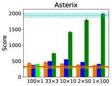
(b)

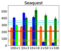
(c)

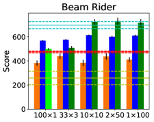
(d)

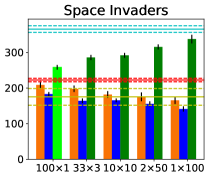
(e)

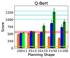
(f)

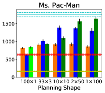
(g)

Figure 2: The results of Rollout-Dyna-DQN with the perfect and imperfect models on six games from the ALE. Like the perfect model, using an imperfect model with a rollout length greater than one provides the most benefit. The horizontal lines show the same baseline scores as Figure 1.

4.2 Experiments

For this section, the experimental setup is the same as in the previous sections, but the perfect model has been replaced with an imperfect model. We pre-trained a model with expert data. Then, holding the model fixed, we repeated the experiment above, measuring Rollout-Dyna-DQN’s performance with various planning shapes. Note that because the model is pre-trained on a single dataset, our results cannot be used to draw reliable conclusions about the effectiveness of this specific model-learning approach. Our aim is only to study the impact of model error on Rollout-Dyna-DQN.

The results of applying Rollout-Dyna-DQN with the imperfect, pre-trained model are shown in Figure 2 (blue bars). The perfect model results and baselines are the same as in Figure 1. The orange bars will be described in Section 5.1.

In every game except Space Invaders, we see evidence that Rollout-Dyna-DQN with a learned model can outperform DQN Extra Updates and furthermore that rollouts longer than one step provided the most benefit. The reason the performance was especially poor in Space Invaders is that the model had trouble predicting bullets, which is fundamental to scoring points. Oh et al. Oh et al. (2015a) attribute this flaw to the low error signal produced by small objects, which can make it difficult to learn about small details in the image. In Seaquest the learned model curiously seems to sometimes outperform the perfect model. Recall that the learned model is trained on expert data – perhaps it is overfitting in a way that happens to be beneficial to planning.

The results also support our hypothesis that there is a trade-off between the benefits of long rollouts for planning and the model’s error increasing with rollout length. For example, in Asterix the performance peaked at 10x10 planning and dropped off as rollouts became shorter or longer. Similarly, in most other games the best-performance was achieved at medium rollout length. In order to ensure that these observations are not specific to this particular learned model, we trained two additional models using the same neural net architecture but different training protocols. Qualitatively we observed similar phenomena: planning shape plays a significant role in performance and trades off with model error in long rollouts. The details and results from those experiments may be found in the online appendix.

The trends are certainly not as clear as with the perfect model; because of the tradeoff with model accuracy, the optimal rollout length will certainly depend on both the problem and the modeling approach. Nevertheless the conclusion remains: planning shape can significantly impact performance and is thus an important consideration for Dyna agents.

5 Planning and Learning Online

In all the experiments so far, a perfect model or a pre-trained learned model has been used; the obvious next step is to study Rollout-Dyna-DQN in the case where the model is learned alongside the value function. Learning the model and value function together adheres to the original conception of Dyna, and also allows us to investigate whether learning a model can improve sample efficiency in this context.

It should be noted that learning the model online raises a host of complex concerns (Ross and Bagnell Ross and Bagnell (2012) offer a theoretical discussion of some of these issues). For instance, exploration becomes especially critical, lest initial model errors cause agent behavior that fails to visit states where the errors occur (ensuring that they will never be corrected). Also, since both the model and the behavior policy are constantly changing, they effect one another in complex and non-stationary ways (this may at times be advantageous or disadvantageous). In this work we do not attempt to substantively address these issues. We primarily seek to evaluate the impact of planning shape on a full-fledged Dyna agent. In so doing, we may also gain insight regarding the viability of this approach with a relatively simple agent architecture.

5.1 Experiments

The experimental setup was the same as in the previous experiments with Rollout-Dyna-DQN, except the model was learned online alongside the value function (training details are available in the online appendix). The results for the six games compared to the pre-trained and perfect models are shown in Figure 2 (orange bars). The main observation is that, as with the perfect and pre-trained models, the best performance was achieved using rollouts longer than one step (except in Space Invaders).

Furthermore, though performance with the online-learned model is generally worse than with the pre-trained model, in three games (Asterix, Seaquest, and Ms. Pac-Man), it was consistently above DQN Extra Updates. Thus, despite the potential pitfalls, we observe that in some cases there is a modest sample efficiency advantage to learning and planning with a dynamics model online over re-using the agent’s prior experience. To our knowledge, this is the first time that this has been demonstrated in the ALE, which has proven to be very challenging for model-based approaches Machado et al. (2017). While this specific instantiation of Dyna is not a plausible competitor to successful model-free agents in this domain, our results suggest that Dyna-style planning is a viable approach that, with further study, may lead to more successful model-based agents. Importantly, the key finding of this paper is that, even if model quality is significantly improved, planning shape must be a consideration in order to get the most out of the learned model.

6 Conclusions and Future Work

Despite the introduction of increasingly effective approaches for learning predictive models in Atari Games Bellemare et al. (2013b, 2014); Oh et al. (2015a), this is the first time that a sample efficiency benefit has been obtained from learning and planning with a dynamics model in this challenging domain. The results show that Dyna is a promising approach for model-based RL in high-dimensional state spaces. However, we also found that the benefit of Dyna-style planning is limited when model-generated experience takes only one step away from the agent’s stored experience, as in the original Dyna-Q. To get the most value from model-based updates, the model must be used to generate novel experience. We found that using the model to generate fewer, longer rollouts was an effective way to achieve this. This finding seems to be robust across different concrete instantiations of Dyna — our results indicate that planning shape has a notable impact on the benefit of planning with different value learners, multiple pre-trained models, and a model learned online along with the value function. The findings in this work also suggest multiple next steps.

We found that the optimal rollout length was unpredictable with imperfect models, as it depends on the model’s reliability in long rollouts. Our results suggest that it would be valuable to develop methods that could adaptively select planning shape, perhaps by monitoring model accuracy in some way.

Some of the model flaws observed by Oh et al. Oh et al. (2015a) were harmful for planning; perhaps improvements in architecture could benefit MBRL performance. Our results show, however, that the benefits of more accurate models will be most apparent when using longer rollouts — even with a perfect model the value of one-step planning is limited.

In the experiments, start states for planning were selected from a buffer containing the agent’s recent real history; it would be interesting to generate promising or interesting start states that may not have been visited by the agent. This would likely involve learning a generative model of the states, which might be accomplished with a solution like a variational autoencoder Kingma and Welling (2013) or a generative adversarial network Goodfellow et al. (2014).

Finally, though longer rollouts were found to be an effective way to use the model to generate experience, there are other promising approaches. For instance one might use inverse dynamics models Pan et al. (2018); Goyal et al. (2018) to effectively propagate value updates backwards in a manner similar to prioritized sweeping Moore and Atkeson (1993); Peng and Williams (1993). It may be possible to combine these insights, exploiting a forward model’s ability to reveal novel states and a backward model’s ability to efficiently improve the value function.

Appendix A Rollout-Dyna-Sarsa Results

In addition to the experiments with DQN and Rollout-Dyna-DQN, we also conducted similar experiments using Sarsa Rummery and Niranjan [1994]; Sutton [1996] with linear function approximation and Blob-PROST features Liang et al. [2016]. We used the same hyper-parameters as Liang et al. Liang et al. [2016], except we set $\lambda=0$, instead of $\lambda=0.9$, to better isolate the effects of planning shape from any interactions with eligibility traces.

We implemented Rollout-Dyna-Sarsa by performing $n$ rollouts, of $k$ steps, after every real step taken by the agent. After every step of the rollout, the value function was updated using the normal Sarsa update rule. The start states for planning were selected uniformly randomly from the 10k most recent states experienced by the agent. For these experiments we assumed the agent had access to a perfect model. The results are shown in Figure A.3. The reported scores are the mean for each algorithm in 100 evaluation episodes after learning for 10M combined real and model frames, and are an average of thirty independent runs.

The model-free baselines that we compared to are similar to the ones used for Rollout-Dyna-DQN. Sarsa 100k (yellow line in Figure A.3) is a Sarsa agent trained for 100k real frames. Sarsa Extra Updates (red line in Figure A.3) is the same as Sarsa 100k, except after every real step it does 100 extra updates using experiences sampled from the agent’s recent history. Sarsa 10M (cyan line in Figure A.3) is a Sarsa agent trained for 10M real frames.

Similar to Rollout-Dyna-DQN, 100$\times$1 planning failed to outperform Sarsa Extra Updates. Also, in every game there was a planning shape with a rollout length greater than one that outperformed both 100$\times$1 planning and Sarsa Extra Updates. These results demonstrate that this phenomenon is not specific to only DQN.

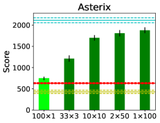
(a)

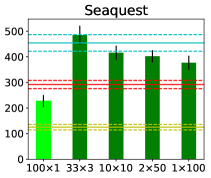
(b)

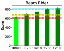
(c)

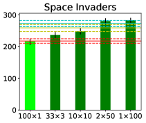
(d)

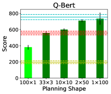
(e)

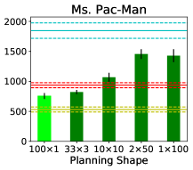
(f)

Figure A.3: The results of running Rollout-Dyna-Sarsa on six games from the ALE compared to the baselines. There is a planning shape with a rollout length greater than one that outperforms both 100$\times$1 and Sarsa Extra Updates (red line) across all the games.

Appendix B Imperfect Model Details

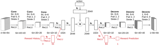
Figure B.4: Oh et al.’s Oh et al. [2015a] action-conditional video prediction model (black) and its extension to predict the next reward (red).

This appendix provides additional details about the deep-neural network that was used for the imperfect model, used in Sections 4 and 5. The architecture is based on the one introduced by Oh et al. Oh et al. [2015a]. This model was shown to make visually accurate predictions for hundreds of steps on video input from Atari games conditioned on actions.

The model encodes a stack of four grayscale frames into a feature vector using a series of convolutional layers. The effect of the action is applied via a multiplicative interaction between the feature vector and the action. After the action transformation, the resulting vector is decoded using a series of deconvolutions before finally outputting the single next frame. The model can be used to make $k$-step predictions by concatenating the predicted frame with the most recent three history frames, and running the model forward another step. A diagram of the model is shown in Figure B.4 (in black).

To train the model, Oh et al. Oh et al. [2015a] created a training data set by running a trained DQN agent and recording the actions and frames. Then, batches of image histories, actions, and image targets are drawn and used to train the model to minimize the average squared error between the predicted and target frames (denoted $\hat{\mathbf{x}}$ and $\mathbf{x}$ respectively) over the $k$-steps. To increase stability during training a curriculum approach is used: the model is first trained to make 1-step, 3-step, then 5-step predictions.

In its original formulation the model predicts only the next state, but an environment model for reinforcement learning needs to predict both the next state and the next reward. Therefore, we extend the model to make reward predictions by adding a separate fully connected layer after the action transformation, followed by an output layer that predicts a single scalar reward (shown in red in Figure B.4). Thus, in addition to the $k$-step image reconstruction loss, the model is trained to minimize the $k$-step squared difference between the predicted, and target rewards ($\hat{r}$ and $r$ respectively):

$$\mathcal{L}_{k}(\boldsymbol{\theta})=\frac{1}{2k}\sum^{k}_{\kappa=1}\left(\left\lVert\mathbf{\hat{x}}_{\kappa}-\mathbf{x}_{\kappa}\right\rVert^{2}+\left\lVert\hat{r}_{\kappa}-r_{\kappa}\right\rVert^{2}\right).$$ (1)

This approach is similar to what was used by Leibfried et al. Leibfried et al. [2017] to jointly predict frames and rewards. As input, we also provide the reward history for the three transitions associated with the input frames. After the reward history input layer, there is a fully connected layer, before joining with the output of the encoder at the action transformation. Since DQN clips the rewards to the interval $[-1,1]$, the input and target rewards for the model are also clipped to the same interval. We used this new architecture to train three different models for each game.

Appendix C Details of Learned Model Training and Additional Results

(a)

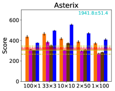
(b)

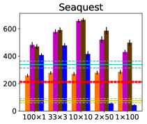
(c)

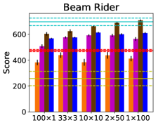
(d)

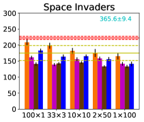
(e)

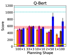
(f)

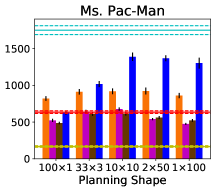
(g)

Figure C.5: Rollout-Dyna-DQN with the learned models, on six games from the ALE.

In addition to the pre-trained learned model used for the experiments presented in Section 4. We pre-trained two additional models and repeated the experiments to ensure that any trends that were observed were not specific to a particular model. Note that because each model is pre-trained on a single dataset, our results cannot be used to draw reliable conclusions about the comparative effectiveness of the different training regimes. Our aim is only to study the impact of model error on Rollout-Dyna-DQN. As such, we refer to the models merely as Models A, B, and C; Model C is the one whose results are presented in Section 4. The results of applying Rollout-Dyna-DQN with the three imperfect models are shown in Figure C.5. The baselines are the same as in Figures 1 and 2. The results demonstrate that the observed trends — rollouts longer than one step provided the most benefit and planning shape plays a significant role in performance — are not unique to a particular instantiation of the model.

To train the models, a procedure similar to what was used by Oh et al. Oh et al. [2015a] was employed. In addition to the extension of the architecture to enable reward prediction, there were also two other changes from the original description. Instead of RMSProp Tieleman and Hinton [2012], the Adam optimizer was used Kingma and Ba [2015], which Oh et al. Oh et al. [2015b] found converged more quickly. And for preprocessing the images, instead of computing and subtracting a pixelwise mean, the mean value per channel was computed and subtracted (grayscale has one channel), following Chiappa et al. Chiappa et al. [2017].

Model A. For each game, a single DQN agent was trained for 10M emulator frames. The trained agent was then run for a series of episodes without learning, and 500k transitions (frames, actions, next frames, and rewards) were recorded to create the training set. The model was then trained, using the training set, for 1M updates with a 1-step prediction loss (batch size 32, learning rate $1\times 10^{-4}$), followed by 1M updates with a 3-step prediction loss (batch size 8, learning rate $1\times 10^{-5}$), for a total of 2M updates.

Model B. The procedure and training data was exactly the same as for Model A, except that it was trained for an additional 1M updates using a 5-step prediction loss (batch size 8, learning rate $1\times 10^{-5}$), for a total of 3M updates.

Model C. For this model, several independent DQN agents at different times during their learning were used to collect the training data. For each game, five independent DQN agents were trained for 10M frames. Then, 25k transitions were recorded from evaluation episodes using a snapshot of each agent at 2.5M, 5M, 7.5M, and 10M frames during their learning. The resulting 500k transitions were then combined to create the training set. The model was then trained for 1M updates with a 1-step prediction loss (batch size 32, learning rate $1\times 10^{-4}$), followed by 500k updates with a 3-step prediction loss (batch size 8, learning rate $1\times 10^{-5}$), then finally 500k updates using a 5-step prediction loss (batch size 8, learning rate $1\times 10^{-5}$), for a total of 2M updates.

Online Learned Model. To train the model online, batches of data are sampled from the agent’s real experience in the experience replay buffer. The model is first trained on 1-step predictions using a learning rate of $1\times 10^{-4}$ for 125k updates (500k agent steps, with training occurring every 4 steps), before switching to 3-step predictions with a learning rate of $1\times 10^{-5}$. The batch size is 32 for both phases of training.

References

- Bellemare et al. [2013a] Marc G. Bellemare, Y. Naddaf, J. Veness, and M. Bowling. The arcade learning environment: An evaluation platform for general agents. Journal of Artificial Intelligence Research, 47:253–279, 2013.
- Bellemare et al. [2013b] Marc G. Bellemare, Joel Veness, and Michael Bowling. Bayesian learning of recursively factored environments. In Proceedings of the 30th International Conference on Machine Learning, pages 1211–1219. PMLR, 2013.
- Bellemare et al. [2014] Marc G. Bellemare, Joel Veness, and Erik Talvitie. Skip context tree switching. In Proceedings of the 31st International Conference on Machine Learning, pages 1458–1466. PMLR, 2014.
- Chiappa et al. [2017] Silvia Chiappa, Sébastien Racaniere, Daan Wierstra, and Shakir Mohamed. Recurrent environment simulators. Conference paper at the International Conference on Learning Representations 2017, 2017.
- Goodfellow et al. [2014] Ian Goodfellow, Jean Pouget-Abadie, Mehdi Mirza, Bing Xu, David Warde-Farley, Sherjil Ozair, Aaron Courville, and Yoshua Bengio. Generative adversarial nets. In Advances in Neural Information Processing Systems 27, pages 2672–2680. Curran Associates, Inc., 2014.
- Goyal et al. [2018] Anirudh Goyal, Philemon Brakel, William Fedus, Timothy P. Lillicrap, Sergey Levine, Hugo Larochelle, and Yoshua Bengio. Recall traces: Backtracking models for efficient reinforcement learning. CoRR, abs/1804.00379, 2018.
- Gu et al. [2016] Shixiang Gu, Timothy Lillicrap, Ilya Sutskever, and Sergey Levine. Continuous deep Q-learning with model-based acceleration. In Proceedings of The 33rd International Conference on Machine Learning, pages 2829–2838. PMLR, 2016.
- Hessel et al. [2018] Matteo Hessel, Joseph Modayil, Hado van Hasselt, Tom Schaul, Georg Ostrovski, Will Dabney, Dan Horgan, Bilal Piot, Mohammad Azar, and David Silver. Rainbow: Combining improvements in deep reinforcement learning. In AAAI Conference on Artificial Intelligence, 2018.
- Kalweit and Boedecker [2017] Gabriel Kalweit and Joschka Boedecker. Uncertainty-driven imagination for continuous deep reinforcement learning. In Proceedings of the 1st Annual Conference on Robot Learning, pages 195–206. PMLR, 2017.
- Kingma and Ba [2015] Diederik P. Kingma and Jimmy Ba. Adam: A method for stochastic optimization. Conference paper at the International Conference on Learning Representations 2015, 2015.
- Kingma and Welling [2013] Diederik P Kingma and Max Welling. Auto-encoding variational bayes. arXiv preprint arXiv:1312.6114, 2013.
- Leibfried et al. [2017] Felix Leibfried, Nate Kushman, and Katja Hofmann. A deep learning approach for joint video frame and reward prediction in atari games. Presented at the ICML 2017 Workshop on Principled Approaches to Deep Learning, 2017.
- Liang et al. [2016] Yitao Liang, Marlos C. Machado, Erik Talvitie, and Michael Bowling. State of the art control of Atari games using shallow reinforcement learning. In Proceedings of the 15th International Conference on Autonomous Agents and Multiagent Systems, pages 485–493, 2016.
- Lin [1992] Long-Ji Lin. Self-improving reactive agents based on reinforcement learning, planning and teaching. Machine Learning, 8(3-4):293–321, 1992.
- Machado et al. [2017] Marlos C. Machado, Marc G. Bellemare, Erik Talvitie, Joel Veness, Matthew J. Hausknecht, and Michael Bowling. Revisiting the arcade learning environment: Evaluation protocols and open problems for general agents. CoRR, abs/1709.06009, 2017.
- Mnih et al. [2015] Volodymyr Mnih, Koray Kavukcuoglu, David Silver, Andrei A Rusu, Joel Veness, Marc G. Bellemare, Alex Graves, Martin Riedmiller, Andreas K Fidjeland, Georg Ostrovski, et al. Human-level control through deep reinforcement learning. Nature, 518(7540):529–533, 2015.
- Mnih et al. [2016] Volodymyr Mnih, Adria Puigdomenech Badia, Mehdi Mirza, Alex Graves, Timothy Lillicrap, Tim Harley, David Silver, and Koray Kavukcuoglu. Asynchronous methods for deep reinforcement learning. In International Conference on Machine Learning, pages 1928–1937, 2016.
- Moore and Atkeson [1993] Andrew W. Moore and Christopher G. Atkeson. Prioritized sweeping: Reinforcement learning with less data and less time. Machine Learning, 13(1):103–130, 1993.
- Oh et al. [2015a] Junhyuk Oh, Xiaoxiao Guo, Honglak Lee, Richard L Lewis, and Satinder Singh. Action-Conditional Video Prediction using Deep Networks in Atari Games. In Advances in Neural Information Processing Systems 28, pages 2845–2853. Curran Associates, Inc., 2015.
- Oh et al. [2015b] Junhyuk Oh, Xiaoxiao Guo, Honglak Lee, Richard L Lewis, and Satinder Singh. Action-conditional video prediction using deep networks in atari games. https://github.com/junhyukoh/nips2015-action-conditional-video-prediction, 2015.
- Oh et al. [2017] Junhyuk Oh, Satinder Singh, and Honglak Lee. Value prediction network. In Advances in Neural Information Processing Systems 30, pages 6118–6128. Curran Associates, Inc., 2017.
- Pan et al. [2018] Yangchen Pan, Muhammad Zaheer, Adam White, Andrew Patterson, and Martha White. Organizing experience: a deeper look at replay mechanisms for sample-based planning in continuous state domains. In Proceedings of the Twenty-Seventh International Joint Conference on Artificial Intelligence, pages 4794–4800, 7 2018.
- Peng and Williams [1993] Jing Peng and Ronald J. Williams. Efficient learning and planning within the Dyna framework. Adaptive Behavior, 1(4):437–454, 1993.
- Peng et al. [2018] Baolin Peng, Xiujun Li, Jianfeng Gao, Jingjing Liu, and Kam-Fai Wong. Deep Dyna-Q: Integrating planning for task-completion dialogue policy learning. CoRR, abs/1801.06176, 2018.
- Ross and Bagnell [2012] Stephane Ross and Drew Bagnell. Agnostic system identification for model-based reinforcement learning. In Proceedings of the 29th International Conference on Machine Learning (ICML), pages 1703–1710, 2012.
- Rummery and Niranjan [1994] G. A. Rummery and M. Niranjan. On-line Q-learning using connectionist systems. Technical report, CUED/F-INFENG/TR 166, Engineering Department, Cambridge University, 1994.
- Sutton [1990] Richard S. Sutton. Integrated architectures for learning, planning, and reacting based on approximating dynamic programming. In Machine Learning Proceedings 1990, pages 216 – 224. Morgan Kaufmann, 1990.
- Sutton [1996] R. S. Sutton. Generalization in reinforcement learning: Successful examples using sparse coarse coding. In Advances in Neural Information Processing Systems 8, pages 1038–1044. MIT Press, 1996.
- Talvitie [2014] Erik Talvitie. Model regularization for stable sample rollouts. In Proceedings of the 30th Conference on Uncertainty in Artificial Intelligence, pages 780–789, 2014.
- Tamar et al. [2016] Aviv Tamar, Yi Wu, Garrett Thomas, Sergey Levine, and Pieter Abbeel. Value iteration networks. In Advances in Neural Information Processing Systems 29, pages 2154–2162. Curran Associates, Inc., 2016.
- Tieleman and Hinton [2012] T. Tieleman and G. Hinton. Lecture 6.5 – RMSProp: Divde the gradient by a running average of its recent magnitude. In Neural Networks for Machine Learning. Coursera, 2012.
- Weber et al. [2017] Theophane Weber, Sébastien Racanière, David Reichert, Lars Buesing, Arthur Guez, Danilo Jimenez Rezende, Adrià Puigdomènech Badia, Oriol Vinyals, Nicolas Heess, Yujia Li, Razvan Pascanu, Peter Battaglia, Demis Hassabis, David Silver, and Daan Wierstra. Imagination-augmented agents for deep reinforcement learning. In Advances in Neural Information Processing Systems 30, pages 5690–5701. Curran Associates, Inc., 2017.