A Novel Side-Channel in Real-Time Schedulers

Abstract

We demonstrate the presence of a novel scheduler side-channel in preemptive, fixed-priority real-time systems (RTS); examples of such systems can be found in automotive systems, avionic systems, power plants and industrial control systems among others. This side-channel can leak important timing information such as the future arrival times of real-time tasks. This information can then be used to launch devastating attacks, two of which are demonstrated here (on real hardware platforms). Note that it is not easy to capture this timing information due to runtime variations in the schedules, the presence of multiple other tasks in the system and the typical constraints (e.g., deadlines) in the design of RTS. Our ScheduLeak algorithms demonstrate how to effectively exploit this side-channel. A complete implementation is presented on real operating systems (in Real-time Linux and FreeRTOS). Timing information leaked by ScheduLeak can significantly aid other, more advanced, attacks in better accomplishing their goals.

I Introduction

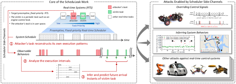
Figure 1: Overview of paper: We demonstrate how an unprivileged, low-priority task (in user space) can use the ScheduLeak algorithms to infer execution behaviors of critical, high-priority periodic task(s). The extracted information is useful for helping other attacks achieve their primary goals (two such attack instances are implemented in this paper as possible use cases).

Consider the scenario where an adversary wants to attack an embedded real-time system (RTS) – parts of autonomous cars, industrial robots, anti-lock braking systems in modern cars, unmanned aerial vehicles (UAVs), power grid components, the NASA rovers, implanted medical devices, etc. These systems typically have limited memory and processing power, have very regimented designs (stringent timing constraints for instance) and any unexpected actions can be quickly thwarted. Therefore, the opportunity to either steal a critical piece of information or the ability to launch that attack which takes control of the system can be very limited. As a consequence, attacks on such systems require significant system specific information. This “information” can take many forms – from an understanding of the design of the system, to knowledge of the critical components (either software or hardware). The exact knowledge depends on the type of attack and the target component. For example, say, (a) to steal important information about when (and where) an on-board camera is used for reconnaissance or (b) to take control away from the ground operator of a remotely-controlled vehicle.

The one common underlying theme that pervades real-time systems (and something that a would-be attacker should definitely address) is the importance of timing. “Timing” includes: (i) when certain events occur, (ii) how often they occur, and, most importantly for this paper, (iii) when (and if) they will occur again in the future. In fact, a number of critical software components in real-time systems are periodic in nature. As we shall see, these periodic tasks present themselves as prime targets for attackers.

So, how does one attack such systems, especially the periodic (and critical) components?

We have discovered the presence of a scheduler-based side-channel that leaks timing information in real-time systems – in particular those with fixed priority tasks.

The scheduler-based side-channel enables an unprivileged, low-priority task to learn the precise timing behavior of the critical, periodic (victim) task(s) by simply observing its own execution intervals using a system timer. This provides an attacker with the ability to infer the initial offset of the victim task and precisely predict its future arrival times at runtime. We name the algorithms that exploit this side-channel attack, “ScheduLeak”.

Figure 1 presents an overview of the side-channel and also how the attacker can benefit from the scheduler side-channel-based information. The left side of the figure shows how a real-time system consisting of fixed-priority tasks (the boxes at the top – the victim is a periodic task while all other tasks can be either periodic or sporadic) that results in a schedule (dotted boxes in the middle, with each task being indistinguishable from the other at runtime) can be analyzed to extract the precise future arrival time points (the green, upward arrows) of the victim task. The right-hand side of the figure shows how this timing information of the critical task can be used to launch other attacks that either leak more important information or destabilize the real-time control system. Note that without this precise timing information, an attacker is either forced to guess when the victim task(s) will execute or launch the attacks at random points in time – both of which dilute the efficacy of the attack or result in early termination of the system.

The extraction of this runtime timing information is non-trivial; main reasons include (a) the runtime schedule depends heavily on the state of the system at startup, initialization variables and environmental conditions and (b) real-time systems typically include multiple non-real-time tasks as well. Even precise knowledge of all statically-known system parameters is insufficient to reconstruct the future arrival times of the victim. While a privileged attacker could target the scheduler of the system and extract the requisite information, such access typically requires significant effort and/or resources. On the other hand, we are able to reconstruct the information with the same level of precision using an unprivileged user space application. This is achieved by letting the attacker’s application keep track of its own scheduling information. Coupled with some easily obtainable information about the system (e.g., the victim task’s period), the attacker can recreate the targeting timing information with high precision.

To be more specific, let’s say that we want to override the (remote) control of a rover. In many such systems, a periodic pulse width modulation (PWM) task drives the steering and throttle. Without knowledge of when the PWM task is likely to update the motor control values, the attacker is forced to employ brute force or random strategies to override the PWM values. These could either end up being ineffective or lead to the entire system being reset before the attack succeeds (see Section VI for more details on this and another scenario). Armed with knowledge from ScheduLeak, our smart adversary can now override the PWM values right after they have been written by the corresponding task – effectively overriding the actuation commands.

Scheduler covert channels, where two processes covertly communicate using the scheduler, have long been known (e.g., [1, 2, 3]). In contrast, our focus is on a side-channel that leaks execution timing behavior (not deliberately, as opposed to the scheduler covert channels) of critical, high-priority real-time tasks to unprivileged, low-priority tasks. We focus on uniprocessor (i.e., single-core) systems with a preemptive, fixed-priority real-time task scheduler [4, 5] since they are the most common class of real-time systems deployed in practice today [6]. It is important for an attacker to stay within the strict execution time budgets allotted to the unprivileged task – especially during the phases when it is trying to observe and reconstruct the victim’s timing behavior. Failing this requirement will likely cause other critical real-time functionality to fail or trigger a watchdog timeout that resets the system, leading to premature ejection of the attacker. This property is crucial during the ‘reconnaissance’ phase of what has come to be known as advanced persistent threat (APT) attacks [7, 8]. E.g., it has been reported that attackers had penetrated and stayed resident undetected in the system for months before they initiated the actual attack in the case of Stuxnet [9]. Once they had enough information about system internals, they were able to craft effective attacks tailored to that particular system.

The ScheduLeak algorithms are implemented on both: (a) real hardware platforms running Real-Time Linux and FreeRTOS (for the two attack case studies) and (b) a simulator. We evaluate the performance and scalability of ScheduLeak in Section VII, along with a design space exploration (on the simulator). The results show that our methods are effective at reconstructing schedule information and provide valuable information for later attacks to better accomplish their attack goals. To summarize, the main contributions are:

1. Novel scheduler side-channel attack algorithms that can accurately reconstruct the initial offsets and predict future arrival times of critical real-time tasks in real-time systems (without requiring privileged access) [Section III]

2. Analyses and metrics to measure the accuracy in predicting the execution and timing properties of the victim tasks [Sections IV and VII].

3. Implementation and case studies on real hardware platforms (i.e., autonomous systems) running Real-time Linux and FreeRTOS [Section VI].

II System and Adversary Model

II-A Time Model

We assume that the attacker has access to a system timer on the target system and therefore time measured by the attacker has the resolution equal to this system timer. The timer can be either a software or a hardware timer (e.g., a 64-bit Global Timer in FreeRTOS or a $\mathtt{CLOCK\_MONOTONIC}$-based timer in Linux). We consider a discrete time model [10]. We assume that a unit of time equals a timer tick (of the timer that the attacker can access) and the tick count is an integer. All system and task parameters are multiples of a time tick. We denote an interval starting from time point $a$ and ending at time point $b$ that has a length of $b-a$ by $[a,b)$ or $[a,b-1]$.

II-B System Model

We consider a uniprocessor (i.e., single-core), fixed-priority, preemptive real-time system consisting of $n$ real-time tasks $\Gamma=\{\tau_{1},...\tau_{n}\}$. A task can be either a periodic or a sporadic task. Each task $\tau_{i}$ is characterized by $(p_{i},d_{i},e_{i},a_{i},pri_{i})$ where $p_{i}$ is the period (or the minimum inter-arrival time), $d_{i}$ is the relative deadline, $e_{i}$ is the worst-case execution time (WCET), $a_{i}$ is the initial task offset (i.e., the arrival time) and $pri_{i}$ is the priority. We assume that every task has a distinct period and that a task’s deadline is equal to its period [5]. We use the same symbol $\tau_{i}$ to represent a task’s job (or instance) for simplicity of notation. We assume that task release jitter is negligible. Thus, any two adjacent arrivals of a periodic task $\tau_{i}$ has a constant distance $p_{i}$. We further assume that each task is assigned a distinct priority and that the taskset is schedulable by a fixed-priority, preemptive real-time scheduler. Let $hp(\tau_{i})$ denote the set of tasks that have higher priorities than that of $\tau_{i}$ and $lp(\tau_{i})$ denote the set of tasks that have lower priorities than $\tau_{i}$. We define an “execution interval” of a task to be an interval of time $[a,b)$ during which the task runs continuously. If $\tau_{i}$ is preempted then the execution will be partitioned into multiple execution intervals, each of which has length less than $e_{i}$.

Table I: A summary of the system and adversary model.

Real-Time System Assumptions
A1	A preemptive, fixed-priority real-time scheduler is used.
A2	The victim task is a periodic task.
Attacker’s Capabilities (Requirements)
R1	The attacker has the control of one user-space task (observer
	task) that has a lower priority than the victim task.
R2	The attacker has knowledge of the victim task’s period.
R3	The attacker has access to a system timer on the system.
Attacker’s Goals
G1	Infer the victim task’s initial offset and predict future arrivals.

II-C Adversary Model

We assume that an attacker is interested in targeting one of the critical tasks in the system that we henceforth refer to as a “victim task”, denoted by $\tau_{v}\in\Gamma$. We also assume that $\tau_{v}$ is a real-time, periodic task. Many critical functions in real-time control systems are periodic in nature, e.g., the code that controlled the frequency of the slave variable-frequency drives in the Stuxnet example [9]. In all such cases, the period of the task is strictly related to the characteristics of the physical system and thereby can be deduced from the physical properties; hence, we can assume that the attacker is able to gain knowledge of the victim task’s period beforehand. It is common that, before attacking complex systems (e.g., CPS), adversaries will study the design and details of such systems. However, the attacker does not know the initial conditions at system start-up (e.g., the task’s initial offset) and may not have information on all the tasks in the system. All other tasks in the system can be either periodic, sporadic or non-real-time, depending on the design of the system. Hence, the methods developed in this paper can target systems that have a mix of periodic, sporadic and non-real-time tasks.

The ultimate goal varies with adversaries and the systems under attack. For example, in advanced persistent threat (APT) attacks [7, 8], one may plan to interfere with the operations of critical tasks, eavesdrop upon certain information via shared resources or even carry out debilitating attacks at a critical juncture when the victim system is most vulnerable. Oftentimes, such attacks require the attacker to precisely gauge the timing properties of victim tasks. In this paper, we introduce attack algorithms that help an attacker obtain this valuable information during the reconnaissance stage. In this context, the main goal of the attacker is to precisely infer when the victim task is scheduled to run in the near future (i.e., the future arrival times).

Note that our focus in this paper is on how to reconstruct the timing behavior of a higher-priority periodic victim task using the scheduler side-channel without violating the real-time constraints. We do this from the vantage point of a compromised, lower-priority (“observer”) task. We do not focus on how attackers get access to the observer task. They could use any number of known methods – from compromised insiders, to supply chain vulnerabilities in a multi-vendor development model (as is usually practiced for the design and development of large, complex systems such as aircraft, automobiles, industrial control systems, etc.) [11], to vulnerabilities in the software and network among others. Recent work has demonstrated that real-time systems like commercial drones contain design flaws and hence are vulnerable to compromise [12, 13]. The details of gaining access to an observer task are out of scope for this paper. Nevertheless, it is important to note that we do not require the observer task to be a privileged task in the system. A summary of assumptions, attacker’s capabilities and goals is given in Table I.

II-D Observer Task

As previously mentioned, we refer to the lower-priority task that the attacker controls as an “observer task” and it is denoted by $\tau_{o}\in\Gamma$. It can be a user-space task. The only constraint we place on $\tau_{o}$ is that it has a lower priority than the victim task, $pri_{v}>pri_{o}$. The observer task can be either a periodic or a sporadic task and its period (or its minimum inter-arrival time) can be shorter or longer than the victim task. In particular, being a periodic task is a more restrictive condition since it reduces the flexibility available to an attacker (this will be clearer as we introduce the algorithms). That is, the case where a periodic observer task with a period $p_{o}$ and priority $pri_{o}$ can succeed, a sporadic observer task (by picking the same $p_{o}$ as the minimum inter-arrival time and the same priority $pri_{o}$) can also succeed. Therefore, when analyzing the attack capabilities in Section IV, we will consider a periodic observer task (or a sporadic observer task running at a constant inter-arrival time).

In this paper, we use the observer task to infer the initial offset $a_{v}$ that can be used to predict future arrivals of the victim task. We let the observer task “monitor” its own execution intervals by using a system timer. Note that reading system time does not require privilege in most operating systems (e.g., invoking $\mathtt{clock\_gettime()}$ in Linux). The key idea here is that the intervals when the observer task is active cannot contain the victim task’s execution or its arrival time point since the victim would have preempted the observer task. However, there are also other higher-priority tasks that can impact the observer task’s execution behaviors. To the attacker, the challenge is to then filter out unnecessary information and extract the correct information about the victim task. This is explained in the following section.

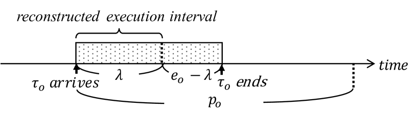
(a) No preemption has occurred.

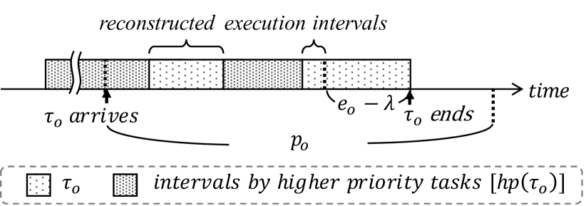
(b) Some tasks $\tau_{i}\in hp(\tau_{o})$ preempt $\tau_{o}$.

Figure 2: Examples of reconstructed execution intervals of the observer task. The total length of the reconstructed execution interval(s) is $\lambda$ that leaves $e_{o}-\lambda$ for $\tau_{o}$ to perform original task functions.

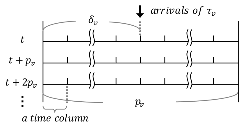
Figure 3: The skeleton of a schedule ladder diagram. The start time $t$ of the diagram (i.e., the beginning of the top timeline) is an arbitrary point in time, assigned by the attacker. The width of each timeline matches the victim task’s period $p_{v}$. The relative offset between the start time $t$ and the true arrival column is defined by $\delta_{v}$.

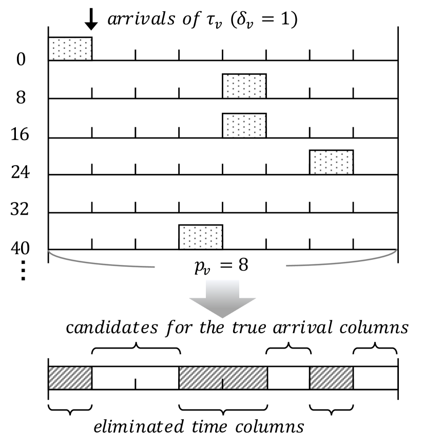
Figure 4: The processed schedule ladder diagram for Example 1.

III ScheduLeak

III-A Overview

We now introduce the core algorithms. The main idea is that the victim task cannot run while the observer task is running since the latter has a lower priority. By reconstructing the observer task’s own execution intervals and analyzing those intervals based on the victim task’s period, we may infer the initial offset and future arrival times for the victim task. A high-level overview of the various analyses stages in our proposed ScheduLeak algorithms includes:

1. Reconstruct execution intervals of the observer task: first, the observer task uses a system timer to measure and reconstruct its own execution intervals (i.e., times when it itself is active). [Section III-B]

2. Analyze the execution intervals: The reconstructed execution intervals are organized in a “schedule ladder diagram” – a timeline that is divided into windows that match the period of the victim task. [Section III-C]

3. Infer the victim task’s initial offset and future arrivals: in the final step, the initial offset for the victim task is inferred. This information is then used to predict the future arrivals of the victim. Since the victim task is periodic in nature, the offset from the start of its own window translates to the offset from startup when the first instance of the victim task executed. [Section III-D]

III-B Reconstruction of Execution Intervals

The first step is to reconstruct the observer task’s execution intervals. We implement a function in the observer task that keeps track of time read from the system timer. By examining the polled time stamps, preemptions (if any) can be identified and the execution intervals of the observer task can be reconstructed. While this function seems straightforward, ensuring that it respects real-time constraints (i.e., all real-time tasks must meet their deadlines) is critical. That is, the observer task should not run more than its WCET, $e_{o}$. Furthermore, even if the attacker does not exceed the allocated execution budget for itself, it may want to save some budget for other purposes such as performing the analyses to reconstruct the timing information of the victim. Hence, we define a parameter, $\lambda$, whose value is set by the attacker, to limit the running time of the aforementioned function for the observer task in each period. This “maximum reconstruction time”, $\lambda$, is an integer in the range $0\leq\lambda\leq e_{o}$. The total length of the reconstructed execution intervals is $\lambda$ in each period and this leaves the timespan $e_{o}-\lambda$ for the observer task to carry out other computations. As a result, the service levels guaranteed by the original (clean) system is still maintained – thus reducing the risk of triggering system errors. On the flip side, the attacker may not be able to capture all possible execution intervals and this could reduce the fidelity/precision of the final results. Section IV-B discusses how to compute good values for $\lambda$. Figure 4 shows examples of reconstructed execution intervals. The function for reconstructing an execution interval of the observer task while taking $\lambda$ into account is detailed in Appendix-A as Algorithm 1.

III-C Analysis of Execution Intervals

Once the observer task’s execution intervals are reconstructed, we analyze the data to extract information about the victim task. We organize the observer’s execution intervals into a timeline split into lengths of the victim task’s period $p_{v}$ (recall that $p_{v}$ is one of the known quantities for the attacker). The purpose of this step is to place the execution intervals of the observer task within periodic windows of the victim task. The timeline split into windows of length that matches the victim task’s period allows the attacker to see how the observer task’s execution intervals are influenced by the victim task as well as other higher-priority tasks.

To better illustrate the idea of the timeline and the proposed algorithms, we will use a “schedule ladder diagram” (defined below) to represent the construction of the timeline in this paper. The rows in the schedule ladder diagram can be merged into a single-line timeline (and is just an analytical “trick”). A schedule ladder diagram is a skeleton consisting of a set of adjacent timelines of equal lengths – that match the victim task’s period $p_{v}$. The start time of the top section can be an arbitrary point in time assigned by the attacker (e.g., the time instant when the algorithms are first invoked). The columns in the schedule ladder diagram are “unit time columns”. So, there are $p_{v}$ time columns. That is, the schedule ladder diagram has the same time resolution as the reconstructed execution intervals. The skeleton of a schedule ladder diagram is illustrated in Figure 4. From the diagram, plotted based on $p_{v}$, we make the following observation:

Observation 1.

Any schedule ladder diagram of $\tau_{v}$ must contain exactly one arrival instance of $\tau_{v}$ in every row. All arrivals of $\tau_{v}$ are located in the same time column.

This observation is true because $\tau_{v}$ is a periodic task that arrives every $p_{v}$ time units and the schedule ladder diagram is plotted with its interval equal to $p_{v}$. We define the column where the arrivals of the victim task are located as the “true arrival column”, denoted by $\delta_{v}$. Thus, the correlation between the initial offset $a_{v}$ and the true arrival column $\delta_{v}$ can be derived by $(t+\delta_{v}-a_{v})\ mod\ p_{v}=0$, where $t$ represents the (arbitrary) start time of the schedule ladder diagram assigned by the attacker. This is also depicted in Figure 4. Based on this observation, we define the following theorem with respect to the observer task’s executions on the schedule ladder diagram:

Theorem 1.

The observer task’s execution intervals do not appear at the time columns $[\delta_{v},\delta_{v}+bcet_{v})$, where $bcet_{v}$ is the best case execution time of $\tau_{v}$.

Proof.

From Observation 1, the victim task $\tau_{v}$ arrives regularly at time column $\delta_{v}$. If there exists lower priority tasks $lp(\tau_{v})$ in execution at $\delta_{v}$ column, the victim task preempts such tasks until it finishes its job with length of $bect_{v}$ at a minimum. In the case that there exists higher priority tasks $hp(\tau_{v})$ that are executing or arriving during $[\delta_{v},\delta_{v}+bcet_{v})$, the victim task $\tau_{v}$ is preempted. Under this circumstance, if the observer task $\tau_{o}$ had arrived during $[\delta_{v},\delta_{v}+bcet_{v})$, as a lower priority task, it is also preempted. Therefore, the time columns $[\delta_{v},\delta_{v}+bcet_{v})$ cannot contain the execution intervals of the observer task. ∎

In other words, the time columns where the observer task $\tau_{o}$ can ever appear are not the true arrival column $\delta_{v}$. To this end, it’s easier to think of the problem as the process of eliminating those such time columns. If we place the obtained execution intervals of $\tau_{o}$ on the schedule ladder diagram and remove the corresponding time columns, then, there must exist at least an interval of continuous time columns, of which the length is equal to or greater than $bcet_{v}$, that is not removed in the end. Those time columns are candidates for the true arrival time of $\tau_{v}$. There may also exist time columns that are not removed due to other higher-priority tasks. Yet, since other tasks have distinct arrival periods (or random arrivals for sporadic tasks), those time columns tend to be scattered (compared to $[\delta_{v},\delta_{v}+bcet_{v})$) and are expected to be eliminated as more execution intervals of the observer task are collected. In practice, our results indicate that this process works effectively and is mostly stabilized after an attack duration of $5\cdot LCM(p_{o},p_{v})$ (see Section VII-B1).

Example 1.

Consider an RTS consisting of four tasks $\Gamma=\{\tau_{1},\tau_{o},\tau_{v},\tau_{4}\}$. For the sake of simplicity, we assume that all tasks are periodic in this example (though our analysis can work with periodic, sporadic and mixed systems as well). The task parameters are presented in the table below (on the left). Note that $pri_{i}>pri_{j}$ means that $\tau_{i}$ has a higher number than $\tau_{j}$. Thus, task $\tau_{1}$ has the lowest priority while task $\tau_{4}$ has the highest priority and $\tau_{v}$ has higher priority than $\tau_{o}$. Let the maximum reconstruction duration $\lambda$ be $1$ and the start time of the attack be $0$ (as a result, $a_{v}$ equals $\delta_{v}$ in this example). Assuming the attacker has executed the first step/algorithm for some duration, the table below lists the reconstructed execution intervals of the observer task.

	$p_{i}$	$e_{i}$	$a_{i}$	$pri_{i}$
$\tau_{1}$	15	1	3	1
$\tau_{o}$	10	2	0	2
$\tau_{v}$	8	2	1	3
$\tau_{4}$	6	1	4	4

Reconstructed

Execution Intervals

[0,1)

[12,13)

[20,21)

[30,31)

[43,44)

Note that since $\tau_{1}$ has priority lower than the observer task $\tau_{o}$, it does not influence the execution of $\tau_{o}$. Then, we place the reconstructed execution intervals in a schedule ladder diagram of width equal to the victim task’s period $p_{v}$. This operation is shown in Figure 4. To better understand the effectiveness of the schedule ladder diagram in profiling the victim task’s behavior, we plot the original, complete, schedule on the ladder diagram in Figure 12 in Appendix so that readers get a better sense of it. This gives us an insight into the relation between the execution intervals of $\tau_{o}$ and that of the victim task.

From the schedule ladder diagram in Figure 4, we remove the time columns that are occupied by the observed execution intervals. The results are shown at the bottom of Figure 4. What’s left are candidate time columns that contain the true arrival times for the victim that we want to extract. These intervals are passed to the final step to infer the initial offset/arrival times of the victim task. $\blacksquare$

III-D Inference of Initial Offset and Future Arrival Instants

We now get to the final step – inferring the future arrival instants of the victim task – our original objective. But, first, we need to calculate the initial offset of the victim task. What we get from the previous step is a set of intervals of candidate time columns that contains the true arrival column of the victim task. The number of intervals depends on the number of collected execution intervals as well as the “noise” introduced by other, higher-priority, tasks (hence, there is no guarantee that all false time columns can be eliminated in the end). However, as observed from our experiments and based on Theorem 1, the false time columns tend to be scattered. Therefore, we take the largest interval as our inference that may contain the true arrival column of the victim task. We then pick the start of this interval as the inferred true arrival column, denoted by $\hat{\delta_{v}}$. While this strategy is not always guaranteed to succeed, our evaluation (both case studies in Section VI and performance evaluation in Section VII) shows that we are able to achieve a high degree of precision for the inference. The required initial offset, denoted by $\hat{a_{v}}$, can then be derived as $\hat{a_{v}}=(t+\hat{\delta_{v}})\ mod\ p_{v}$, where $t$ represents the start time of the schedule ladder diagram.

Example 2.

The intervals obtained from Example 1 correspond to the time columns $[1,3),[5,6)$ and $[7,8)$. According to the algorithm, the largest interval, $[1,3)$, is selected. The starting point of such an interval is then taken as the inference of the victim task’s true arrival column, which becomes $\hat{\delta_{v}}=1$. In this example, the true arrival column is $\delta_{v}=1$. Therefore, the algorithms correctly infer the true arrival column of the victim task and the initial offset can be derived accordingly. $\blacksquare$

Now, the future arrivals of the victim task can easily be computed by $\hat{a_{v}}+p_{v}\cdot T$, $T\in\mathbb{N}$, where $\hat{a_{v}}$ is the inferred initial offset of $\tau_{v}$, $p_{v}$ is the period of $\tau_{v}$ and $T$ is the desired arrival number. The result of this calculation is the exact time of the $T^{th}$ arrival of the victim task.

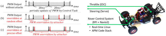
Figure 5: An illustration of PWM channels on a rover system. (a) The PWM outputs are updated periodically by a $50Hz$ task. (b) A naive attack issuing the PWM updates at random instants may not be effective. (c) By carefully issuing the PWM updates right after the original updates, the PWM outputs can be overridden.

IV Analysis of Algorithms

IV-A Analyzing Attack Capability

We now discuss how to determine the attack capability or effectiveness of the observer task with respect to the victim task. That is, in this context, whether the observer task can remove all false time columns, and hence, correctly infer the arrival information of the victim task. Note that the analysis presented in this section focuses on the observer task being a periodic task since, as we mentioned in Section II-D, it is a more restrictive condition to an attacker. Given the same target system, a sporadic observer task may perform better as the sporadic task naturally has more flexible arrivals that are constrained only by its minimum inter-arrival time.

A conservative condition ensuring that all false time columns can be removed from the schedule ladder diagram of $\tau_{v}$ is: when the observer task’s execution intervals appear in all possible time columns. Therefore, we first analyze how the observer task’s execution relates to the victim task’s execution. When considering both $\tau_{v}$ and $\tau_{o}$ as periodic tasks, we have the following observation and theorem:

Observation 2.

In the schedule ladder diagram, the offset between the time column of each observer task’s arrival (i.e., the scheduled execution) and the true arrival column repeats after their least common multiple, $LCM(p_{o},p_{v})$. $\blacksquare$

Theorem 2.

If the given observer task $\tau_{o}$ and the victim task $\tau_{v}$ satisfy the inequality $e_{o}\geq GCD(p_{o},p_{v})$, then the scheduled execution of $\tau_{o}$ is guaranteed to appear in all time columns of the schedule ladder diagram of $\tau_{v}$.

Proof.

From Observation 2, the time column offset of the observer task’s execution repeats every $LCM(p_{o},p_{v})$. Therefore, the aforementioned condition (i.e., the scheduled execution of $\tau_{o}$ appears in all possible time columns) can be described by the inequality $\frac{LCM(p_{o},p_{v})}{p_{o}}\cdot e_{o}\geq p_{v}$. Then, by using $LCM(p_{o},p_{v})=\frac{p_{o}p_{v}}{GCD(p_{o},p_{v})}$, we can derive a condition for $e_{o}$ that guarantees that the observer task can detect the arrivals of the victim task to be $e_{o}\geq GCD(p_{o},p_{v})$. ∎

From Theorem 2, we find that the observer task’s scheduled execution can appear in some of the time columns more than once during $LCM(p_{o},p_{v})$ when $e_{o}>GCD(p_{o},p_{v})$. The redundant coverage means that the false time columns will be visited by $\tau_{o}$ more frequently when compared to the lower ratio of $e_{o}$ to $GCD(p_{o},p_{v})$. In contrast, if $e_{o}<GCD(p_{o},p_{v})$, then not all the false time columns can be covered and examined by the observer task. To better profile the observer task’s coverage, we further define a coverage ratio that depicts the observer task’s capability against the victim task as follows

Definition 1.

(Coverage Ratio) The coverage ratio, denoted by $\mathbb{C}(\tau_{o},\tau_{v})$, is computed by

$$\mathbb{C}(\tau_{o},\tau_{v})=\frac{e_{o}}{GCD(p_{o},p_{v})}$$ (1)

The coverage ratio can be loosely interpreted as the proportion of the time columns where the observer task can potentially appear in the schedule ladder diagram. If all $p_{v}$ time columns can be covered by the observer task, then $\mathbb{C}(\tau_{o},\tau_{v})\geq 1$. Otherwise $0\leq\mathbb{C}(\tau_{o},\tau_{v})<1$.

IV-B Choosing The Maximum Reconstruction Duration $\lambda$

Recall that, the maximum reconstruction duration $\lambda$ is used to limit the amount of execution time (in a period) taken up by the observer task for running the attack algorithms. As the attacker wants to stay stealthy and minimize disruption to the original functionality, it is desirable to use a $\lambda$ value as small as possible. The remaining execution time $e_{o}-\lambda$ can then be used by the attacker to deliver the original functionality of $\tau_{o}$ while making progress on the capturing of execution data. Based on this idea, $\lambda$ can be determined by:

$$\lambda=\begin{cases}GCD(p_{o},p_{v})&\text{if }\mathbb{C}(\tau_{o},\tau_{v})\geq 1\\ e_{o}&\text{otherwise}\end{cases}$$ (2)

In the case of $\mathbb{C}(\tau_{o},\tau_{v})\geq 1$, the observer task has redundant coverage. Since a one-time coverage is sufficient for the observer task to examine all $p_{v}$ time columns, the additional coverage can be traded for other purposes. Otherwise ($\mathbb{C}(\tau_{o},\tau_{v})<1$), the attacker may need to utilize all its computational resource for the attack.

V Evaluation Metrics

To evaluate ScheduLeak, we define the following two metrics:

(i) Inference Success Rate: We define an inference to be successful if attacker is able to exactly infer the victim task’s initial offset (recall from Section III-D that once we know the initial offset, we can easily predict the future arrival instants). Therefore, the result of an inference is either true or false. The inference success rate is an average of the true/false results for a given test condition for a set of task sets.

(ii) Inference Precision Ratio: In the case that the inference is not exact, we define a metric to evaluate the degree of the inference precision (i.e., how close we got to the actual values). In this paper, the inference target is the initial offset of the victim task. We first compute the distance between the inference and the true value by $\epsilon=\left|\hat{a_{v}}-a_{v}\right|$ , where $a_{v}$ is the initial offset of the victim task and $\hat{a_{v}}$ is the inferred initial offset. We then define the inference precision ratio:

Definition 2.

(Inference Precision Ratio) The inference precision ratio, denoted by $\mathbb{I}_{v}^{o}$, is computed by

$$\mathbb{I}_{v}^{o}=\begin{cases}1-\frac{p_{v}-\epsilon}{\frac{p_{v}}{2}}&\text{if }\epsilon>\frac{p_{v}}{2}\\ 1-\frac{\epsilon}{\frac{p_{v}}{2}}&\text{otherwise}\end{cases}$$ (3)

The inference precision ratio is a real number within $0\leq\mathbb{I}_{v}^{o}\leq 1$. It allows us to know how close the inference is to the true initial offset. $\mathbb{I}_{v}^{o}=1$ indicates that the inference of the initial offset $a_{v}$ is absolutely correct.

VI Evaluation Using Case Studies
on Real Platforms

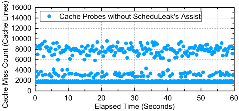
(a) Attack without ScheduLeak’s assist.

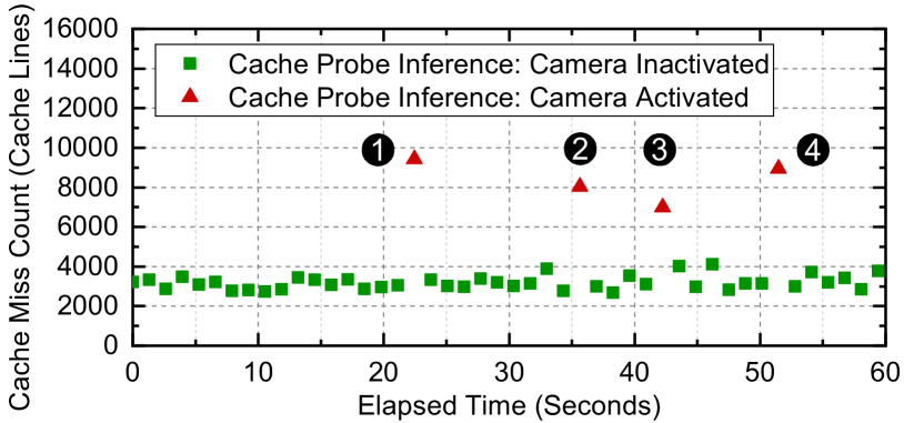
(b) Attack with ScheduLeak’s assist.

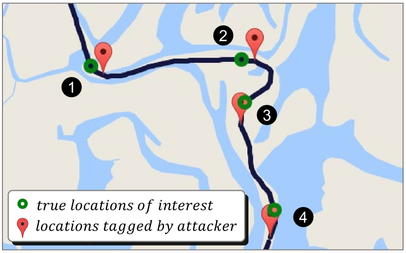
(c) HIL simulator recorded data.

Figure 6: Results of the cache-timing side-channel attacks in Section VI-B. (a) demonstrates that a random mechanism launching the attack at arbitrary instants will lead to many indistinguishable cache usage results. (b) shows a successful attack in which four camera activation events (numbered by $1$ to $4$) are identified from the cache probes using precise time information (inferred by ScheduLeak). (c) visualizes the UAV’s trajectory (bold line), true locations-of-interest (green circles) and the attacker’s inference (red pins) for the attack (b). The result shows that the attacker’s inference matches the ground truth.

Before evaluating performance of the introduced algorithms, we first aim to evaluate the feasibility of such algorithms on realistic platforms in this section. The ScheduLeak algorithms are implemented on two operating systems with a real-time scheduling capability: (i) Real-Time Linux [14] and (ii) FreeRTOS [15]. In what follows, two attack cases are presented. They benefit from the information obtained by the proposed algorithms and utilize such information to accomplish their primary attack goals. The demo videos for these attack cases can be found at https://scheduleak.github.io/.

VI-A Overriding Control Signals

Attack Scenario and Objective: A large number of real-time control systems encapsulate subsystems that control actuators. For instance, in modern automotive systems, the engine control unit (ECU) controls the valve in the electronic throttle body (ETB) to enable electronic throttle control (ETC). In most unmanned drones, the flight controller manages the rotary speed of the motors via the electronic speed controller (ESC). In these systems, the actuation signals such as PWM signals are periodically updated to guarantee a fast and consistent response for the control mission.

Let’s consider an attacker who wants to be able to stealthily override the control in such systems – for the purpose of bad control by causing misbehavior or even taking over the control of the system for a short time span. To do so, the attacker gets into the system as a malicious task and tries to override the control signals. A brute force strategy of excessively overriding the control signals will not work in this scenario because its high attack overhead can cause other real-time tasks to miss their deadlines and lead to a system crash. In this case, knowledge of exact timing when the control signals are updated and overriding them at the right instants allow the attacker to effectively take control with a low overhead.

Implementation: We implement this attack on a custom rover. Its control system is built with a Raspberry Pi 3 Model B board. A Navio2 module board that encapsulates various inertial sensors is attached to the Raspberry Pi board. The system runs Real-Time Linux (i.e., Raspbian, kernel 4.9.45 with PREEMPT_RT patch) with Ardupilot [16] autopilot software suite (one of the most popular open-source code stack in the remote and autonomous control communities). It consists of a set of real-time and non-real-time tasks to perform control-related jobs such as refreshing GPS coordinates, decoding remote control commands, performing PID calculation and updating output signals. One of the tasks periodically updates the PWM values, with a period of $20ms$, for steering and throttle. The updates are sent over Serial Peripheral Interface (SPI) to the Navio2 module that outputs the PWM signals to a servo and a ESC. Figure 5(a) shows an illustration of the PWM output channels working under normal circumstances.

In this attack, we assume that the attacker has access to a low-priority, periodic task (as the observer task, $p_{o}=50ms$) and a non-real-time Linux process (for launching the PWM overriding attack). The attacker’s ultimate objective is to override the control signals updated by the victim task (i.e., the $50Hz$ periodic task). In this implementation, the observer task uses a system call, $\mathtt{clock\_gettime()}$, to obtain clock counts (in nanoseconds) from $\mathtt{CLOCK\_MONOTONIC}$. Time measurement is further rounded up to microseconds when running the ScheduLeak algorithms since all task parameters are multiples of $1us$ in Ardupilot. Once the victim task’s initial offset is determined, the attacker engages the non-real-time process to issue the PWM updates over the same interface that the victim task uses. Note that this is possible due to a lack of authentication between the Raspberry Pi board and the Navio2 module by design. This process keeps track of time by using $\mathtt{clock\_gettime()}$ and issues two PWM updates (one for the steering and one for the throttle) whenever it determines that it has passed a victim task’s arrival instant (i.e., $t-\hat{a_{v}}\ mod\ p_{v}\geq 0$, where $t$ is the present time and $\hat{a_{v}}$ is the inferred victim task’s initial offset). The process remains idle between two PWM updates to reduce the attack footprint.

Attack Results: Figures 5(b) and 5(c) show that the PWM output may be overridden using a different value to the PWM hardware. However, without exact schedule information, the attacker can only periodically send the updates with a randomly selected initial offset (Figure 5(b)). The random initial offset can be any point in the $20ms$ period. From our experiments, only the attack with an initial offset in the range between $a_{v}$ and $a_{v}+8.3ms$ can produce an effective override of the steering and throttle controls. As a result, the attacker has a chance of $41.5\%$ to select a valid initial offset and lead to an effective attack.

On the other hand, the attacker, after launching the ScheduLeak attack and knowing exactly when the victim task arrives, can carefully issue PWM update right after the original update to override the PWM output (Figure 5(c)). In this case, the attacker firstly runs the ScheduLeak algorithms in the observer task, yielding $0.9985$ for the inference precision ratio (for inferring the victim task’s initial offset) in a duration of 1 second. This allows the attacker to launch the PWM overriding attack in the non-real-time process with the precise inference of the victim task’s initial offset. Note that an attacker’s PWM update attempted at a victim task’s arrival instant is executed after the victim task’s job is finished (and hence after the original PWM update) since the non-real-time process has a priority lower than the victim task. Consequently, the attacker can take over control of the steering and throttle. By probing the PWM signals, we observe that the overridden PWM signals are active $85\%$ of the time. As a result, we see that the rover no longer responds to the original control. Instead, the rover is driven by the attacker’s commands. Since the attacker’s task remains idle between two PWM updates, it takes up CPU utilization as small as $2.6\%$.

VI-B Inferring System Behaviors

Attack Scenario and Objective: Let’s consider a UAV system executing a surveillance mission. It captures high resolution images when flying over locations of high-interest. In this case, the attacker’s goal is to extract the locations targeted by the UAV. The strategy is to monitor when the surveillance camera on the UAV is switched to a execution mode in which high-resolution images are being processed. This can be done by exploiting a cache-timing side-channel attack to gauge the coarse-grained memory usage behavior of the task that handles the images. A high cache usage by this task would indicate that a high-resolution image is being processed; otherwise it would use less cache memory. However, a random sampling of the cache will result in noisy (and often useless) data since there exist other tasks in the system that also use the cache. In contrast, knowing when the task is scheduled to run allows the attacker to execute prime and probe attacks [17, 18] very close to the targeted task’s execution.

Implementation: This attack is implemented in a hardware-in-the-loop (HIL) simulation with a Zedboard running FreeRTOS that simulates the control system on a UAV. The system consists of an image processing task (the victim task, $p_{v}=33ms$) handling photos at a rate of $30Hz$ and four other tasks (unknown to the attacker) – all running in a periodic fashion. The victim task processes a large size of data when the UAV reaches a location of interest on a preloaded list. Other tasks consume differing amounts of memory. In this case, we assume that the attacker enters the system as the lowest-priority periodic task, $p_{o}=40ms$. The attacker uses this task for both running the ScheduLeak algorithms and carrying out the cache-timing side-channel attack. The attacker’s final goal is to observe the victim task’s memory usage and learn the system behavior.

Attack Results: First, we consider an attacker who does not employ a ScheduLeak attack. The attacker launches the cache-timing side-channel attack during every period to try and estimate the cache usage of the victim. As shown in Figure 6(a), this produces many cache probes and it is hard to distinguish the cache usage of the victim task from other tasks. This results in an unsuccessful attack since no usage patterns from the victim task can be identified.

Next, let’s consider the case in which the attacker leverages the ScheduLeak attack. In this case, the algorithms yield an inference precision ratio of $0.99$ within a window of $3\cdot LCM(p_{o},p_{v})$ (i.e., 4 seconds). Then, the attacker is able to launch the cache-timing side-channel attack right before and after the victim is executed and skip those instants that are irrelevant. Figure 6(b) shows the result of the precise cache probe against the victim task. We see that the attack greatly reduces the noise caused by other tasks ($96.9\%$ of the cache probes are omitted) and is able to precisely identify the victim task’s memory usage behavior. As a result, four camera activation instants can be identified from the spikes (red triangular points) shown in Figure 6(b). When coupled with the flight route information that the attacker obtains through other measures, it becomes possible to infer the locations of high-interest, as shown in Figure 6(c).

VII Performance Evaluation
and Design Space Exploration

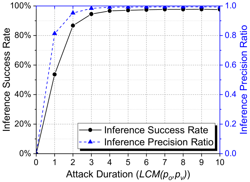
Figure 7: The results of varying attack duration. It indicates that longer attack durations can increase the chance of success and yield better inference precision. The points are connected only as a guide.

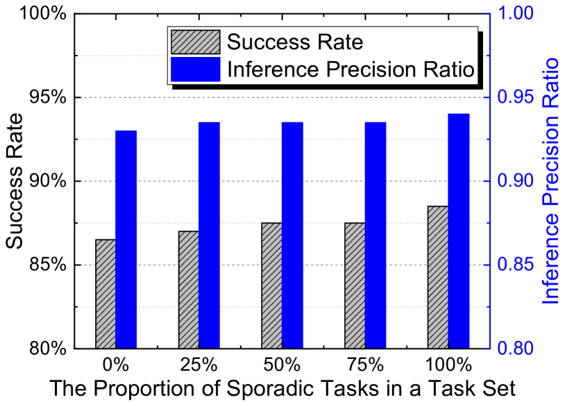
Figure 8: The impact of sporadic tasks. It indicates that the algorithms perform better with sporadic tasks, with a (slightly) ascending trend as the proportion of sporadic tasks increases.

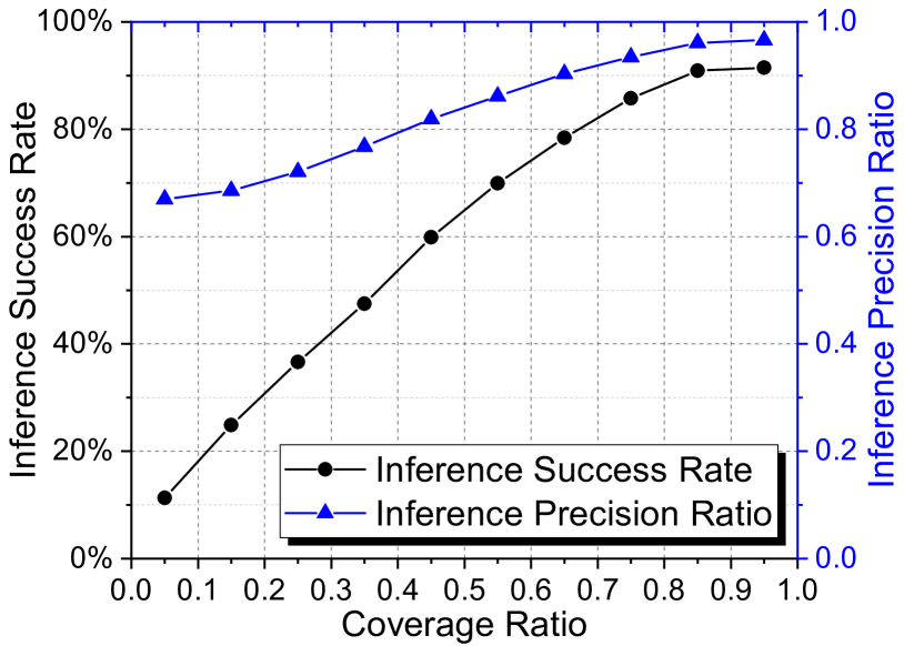
Figure 9: The performance of the algorithms when $\mathbb{C}(\tau_{o},\tau_{v})<1$. Round and triangular points represent the inference success rate and the inference precision ratio, respectively.

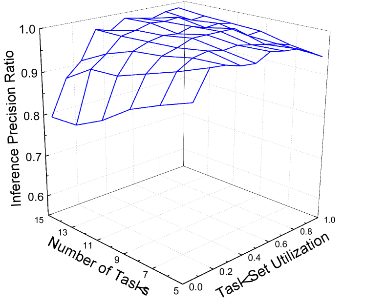
Figure 10: The impact of the number of tasks and the task set utilization. It shows that the algorithms perform better with small number of tasks and high task set utilization.

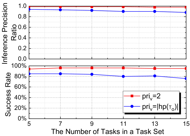
(a) Grouped by the number of tasks.

(b) Grouped by task set utilization.

Figure 11: The impact of the victim task’s position in a task set. It suggests that a victim task with higher priority makes it hard for the algorithms to make a correct inference. This result stands throughout different number of tasks in a task set as well as different task set utilization. Also, a high priority victim task with low task set utilization reduces the inference performance. This explains the huge drop in Figure 11.

VII-A Evaluation Setup

We test our algorithms with randomly generated synthetic task sets. The task sets are grouped by CPU utilization from $[0.001+0.1\cdot x,0.1+0.1\cdot x]$ where $0\leq x\leq 9$. Each utilization group consists of $6$ subgroups that have a fixed number of tasks ($5,7,9,11,13,15$). Each subgroup contains $100$ task sets. In each task set, $50\%$ of the tasks are generated as periodic tasks ($3,4,5,6,7,8$ periodic tasks for each subgroup respectively) while the rest of the tasks are generated as sporadic tasks. The task periods are randomly drawn from $[100,1000]$ and we assume that the attacker has access to the system time with a resolution of $1$. The task initial offset is randomly selected from $[0,p_{i})$. In the case of sporadic tasks, we take the generated task period as the minimum inter-arrival time. The task priorities are assigned using the rate-monotonic algorithm [5]. We only pick those task sets that are schedulable.

The observer task and the victim task are assigned when generating the task sets. In simulations, we consider a periodic observer task because it represents the worst case attack scenario for the adversary, as discussed in Section IV-A. Since only the tasks with higher priorities influence the observations, we skip the generation of lower-priority tasks $lp(\tau_{o})$. Thus, the observer task always has the lowest priority (i.e., $pri_{o}=1$) in these generated task sets. For the victim task, two conditions are considered: (i) $pri_{v}=2$ and (ii) $pri_{v}=\left|hp(\tau_{o})\right|$. This is to test the two boundary conditions. Further, we set the coverage ratio to be $\mathbb{C}(\tau_{o},\tau_{v})\geq 1$ when generating the task sets (except for evaluating the impact of the coverage ratio), to evaluate whether the algorithms can truly produce confident inferences while the attacker has theoretical guarantees of the attack capability (i.e., having full coverage of all $p_{v}$ time columns, as per Theorem 2). The maximum construction duration $\lambda$ is set as per Section IV-B. Thus, $\lambda=GCD(p_{o},p_{v})$.

For varying the execution times of the tasks and adding jitter to the inter-arrival times (for the sporadic tasks), we use the normal and Poisson distributions respectively. Note that Poisson distribution is used for inter-arrival time variation because the probability of each occurrence (i.e., each arrival of the sporadic task) is independent in such a distribution model. First, a schedulable task set is generated (using the aforementioned parameters). Then, for a task $\tau_{i}$, the average execution time is computed by $wcet_{i}\cdot 80\%$. Next, we fit a normal distribution $\mathcal{N}(\mu,\sigma^{2})$ for the task $\tau_{i}$. We let the mean value $\mu$ be $wcet_{i}\cdot 80\%$ and find the standard deviation $\sigma$ with which the cumulative probability $P(X\leq wcet_{i})$ is $99.99\%$. As a result, such a normal distribution produces variation such that $95\%$ of the execution times are within $\pm 10\%\cdot wcet_{i}$. To ensure that the task set remains schedulable, we adjust the maximum modified execution time to be equal to WCET if it exceeds WCET. For sporadic tasks, the average inter-arrival time is computed by $p_{i}\cdot 120\%$. We use a Poisson distribution with $p_{i}\cdot 120\%$ as its mean value to generate the varied inter-arrival times during the simulation. Similarly, so as to not violate the given minimum inter-arrival time for a sporadic task, we regenerate the modified inter-arrival time if it drops below $p_{i}$.

VII-B Results

VII-B1 Attack Duration

Our first goal is to understand the effects of how long attacks last. Recall that the coverage of the schedule ladder diagram repeats every $LCM(p_{o},p_{v})$ (Observation 2). Therefore, we use $LCM(p_{o},p_{v})$ as the unit of time to evaluate the algorithms. Taking the Ardupilot software as an example, the largest $LCM$ of any real-time task (i.e., a AP_HAL thread) pairs is $20ms$. While $LCM(p_{o},p_{v})$ varies system to system, this gives us an insight into the scale of $LCM(p_{o},p_{v})$. In this experiment, we generate task sets as explained in Section VII-A and run the ScheduLeak algorithms with a fixed duration of $10\cdot LCM(p_{o},p_{v})$ for every task set. Figure 9 shows the results of this experiment. In Figure 9, each point of the inference precision ratio is the mean of the individual inference precision ratios of $12000$ task sets for a given attack duration. The results suggest that the longer the attack is sustained, the higher success rate and precision ratio the algorithms can achieve. This is because a longer attack time means more execution intervals are reconstructed by the observer task. On the other hand, both success rate and precision ratio plateau after $5\cdot LCM(p_{o},p_{v})$ with the success rate and the precision ratio higher than $97\%$ and $0.99$ respectively. This shows that the proposed algorithms can produce inference with precision in a very short time and the additional gains obtained from running longer are minuscule. For this reason, we evaluate the algorithms with a duration of $10\cdot LCM(p_{o},p_{v})$ for the rest of the experiments below.

VII-B2 The Number of Tasks and Task Set Utilization

Figure 11 displays a 3D graph that shows the averaged inference precision ratio for each combination of the number of tasks and the task utilization subgroup. The results suggest that (i) the inference precision ratio decreases as the number of tasks in a task set increases and (ii) the inference precision ratio increases as the task set utilization increases. The worst inference precision ratio happens when there are $15$ tasks in a task set with the utilization group $[0.001,0.1]$ – these are boundary conditions for both the number tasks and the utilization in this experiment. The impact of the number of tasks is straightforward as having more tasks in $hp(\tau_{o})$ means that $\tau_{o}$ will be preempted more frequently. This makes it hard for the observer task to eliminate the false time columns. For the impact of the task set utilization, a low utilization value implies that the execution times of the tasks are small and there exists a lot of gaps in the schedule. Hence, the observer may get many small and scattered intervals. Since we let the algorithms pick the largest interval to infer the true arrival column, multiple small intervals are problematic – the algorithm has a hard time picking the right interval that contains the true arrival. Hence errors are compounded.

VII-B3 Priority of the Victim Task

We analyze the impact of the victim task’s priority in a task set. From Section VII-A, we consider two boundary conditions for the victim task’s position: (i) $pri_{v}=2$ and (ii) $pri_{v}=\left|hp(\tau_{o})\right|$. Figures 11(a) and 11(b) present the experiment results for the two conditions. Figure 11(a) shows that the huge drop in Figure 11 (as the number of tasks increases) is mainly caused by the condition $pri_{v}=\left|hp(\tau_{o})\right|$. Figure 11(b) also shows the similar indication that the drop in low utilization groups in Figure 11 is a result of the condition $pri_{v}=\left|hp(\tau_{o})\right|$. It’s worth noting that, since we use the rate-monotonic algorithm to assign the priority, $pri_{v}=2$ means that $\tau_{v}$ has a large period, hence potentially has greater execution time. It benefits the algorithms as we pick the largest interval to make an inference in the final step.

VII-B4 Sporadic and Periodic Tasks

We examine the impact of the mix of sporadic and periodic tasks. We generate task sets with $0\%$, $25\%$, $50\%$, $75\%$ and $100\%$ sporadic tasks in a task set. The rest of the tasks in a task set are periodic tasks. Comparing the result of all periodic tasks and the result of all sporadic tasks shown in Figure 9, we find that the algorithms perform better with more sporadic tasks. It shows an ascending trend as the proportion of sporadic tasks increases. However, the change in the performance is less than $1\%$, which is subtle. Hence, our inference algorithms are fairly agnostic to the actual mix of sporadic/periodic tasks in the system.

VII-B5 Coverage Ratio and The Maximum Reconstruction Duration

The experiments above show that the algorithms can reach certain inference success rates and precision when $\mathbb{C}(\tau_{o},\tau_{v})\geq 1$ and $\lambda=GCD(p_{o},p_{v})$. However, attackers may face a victim system where $\mathbb{C}(\tau_{o},\tau_{v})<1$. That is, the observer task’s execution is not guaranteed to appear in all $p_{v}$ time columns. To evaluate the performance of the algorithms against such a case, we generate task sets with $0<\mathbb{C}(\tau_{o},\tau_{v})<1$ (thus $\lambda=e_{o}$) and run the algorithms for a duration of $10\cdot LCM(p_{o},p_{v})$. In this experiment, task sets are grouped by coverage ratio from $[0.001+0.1\cdot x,0.1+0.1\cdot x]$ where $0\leq x\leq 9$. Figure 9 shows the results. It suggests that the attacker may fail to completely infer the victim task’s initial offset when the coverage ratio is low. Yet, the algorithms can still succeed in some cases due to the fact that Theorem 1 holds even with a low coverage ratio. When the observer has about half coverage of the time columns (the group of $[0.401,0.5]$), it yields $59.9\%$ in success rate and $0.819$ for the averaged inference precision ratio. As more time columns are observed by the observer task, the precision and success rate increase. This is because higher coverage ratios give the algorithms a higher chance to capture the true arrival column and remove others. As a result, the inference success rate is about proportional to the coverage ratio.

VIII Discussion – Potential Defense Strategies

To defend against the proposed attack algorithms, one strategy could be to enforce a low coverage ratio between any low priority task and the critical real-time task by adjusting the task parameters. This reduces the attacker’s observability/capability (based on results from Section VII-B5). Furthermore, carefully designing and employing a harmonic taskset may also reduce ScheduLeak’s inference precision since it creates multiple candidates in the last step of the algorithms. However, any change in the task parameters must fulfill both real-time requirements as well as the required performance. Thus, changing the task parameters may not always be applicable in real-time systems especially the legacy systems that are already deployed.

Since the proposed algorithms rely on the repeating patterns of the victim task, a potential countermeasure is to perturb the periodicity of the system schedule. Yet, the measure will not be trivial due to the real-time constraints of real-time tasks. A careless solution can easily cause some real-time tasks to miss their deadlines and lead to a system failure. A randomization protocol for a rate-monotonic scheduler presented by Yoon et al. [19] is a good attempt on removing the scheduler side-channel for RTS. However, their work is not applicable in our case because they only focus on the systems with all periodic tasks while our work is feasible on the systems with both periodic and sporadic tasks (which is the case in most real-time control systems). Therefore, an effective solution would need to consider covering both task types.

IX Related Work

The problem of information leakage via side-channels has been well studied in the literature. For instance, it has been shown that cache-based side-channels can be invaluable for information leakage [20, 21, 17, 18]. With the advent of multi-tenant public clouds, cache-based side-channels and their defenses have received renewed interest (e.g., [22, 23, 24, 25]). Other types of side-channels such as differential power analysis [26], electromagnetic and frequency analysis [27, 28] have also been studied. Our focus here is on scheduler side-channels in real-time systems.

There has also been some work on information flow via schedulers. The problem where two tasks leak private information by using a covert channel is studied [2, 3]. Völp et al. [1, 29] examined covert channels between different priorities of real-time tasks and proposed solutions to avoid such covert channels. The methodologies for quantifying information leakage in schedulers are also studied [30, 31]. While the previous works focused on covert channels in some schedulers, our focus is on novel side-channels in real-time schedulers where an unprivileged low-priority task can infer the execution timing behaviors of high-priority real-time task(s). Also, in contrast to covert channels that rely on actively preempting real-time tasks, the side-channel in our work does not violate any real-time constraints and the observer task only observes its own behavior.

The integration of security into real-time schedulers is a developing area of research. Mohan et al. [32] offered a consideration of real-time system security requirements as a set of scheduling constraints and introduced a modified fixed-priority scheduling algorithm that integrates security levels into scheduling decisions. Pellizzoni et al. [11] extended the above scheme to a more general task model and also proposed an optimal priority assignment method that determines the task preemptibility. Some researchers also have focused on defense techniques for real-time systems (e.g., [33, 34, 35, 36, 37, 38, 39]). However, these solutions do not protect the systems from the ScheduLeak attack.

The most closely related solution is to adopt a randomization technique to obfuscate the schedule. Yoon et al. [19] introduced a randomization protocol for a preemptive, fixed-priority scheduler that works with only (fully) periodic tasks. Krüger et al.  [40] built upon this by proposing an online job randomization algorithm for time-triggered systems. Nevertheless, these solutions are not applicable to most real-time systems in which a preemptive, fixed-priority scheduler supports both periodic and sporadic real-time tasks. This leaves those systems still vulnerable to our ScheduLeak attack.

X Conclusion

Successful security breaches in control systems (including cyber-physical systems) with real-time properties can have catastrophic effects. In many such systems, knowledge of the precise timing information of critical tasks could be beneficial to adversaries. Our work in this paper demonstrates how to capture this schedule timing information in a stealthy manner – i.e., without being detected or causing any perturbations to the original system. Designers of such systems now need to be cognizant of such attack vectors and design the system to include countermeasures that can thwart potential intruders. The end result is that real-time systems can be more robust to security threats overall.

Appendix

-A Algorithm for Reconstructing An Execution Interval

Algorithm 1 Reconstructing An Execution Interval $\mathbb{E}(e_{o},e_{o}^{\prime},\lambda)$

1:{$GT:global\ timer\ (system\ timer)$}

2:{$e_{o}:the\ worst\ case\ execution\ time\ of\ \tau_{o}$}

3:{$e_{o}^{\prime}:remaining\ execution\ time\ of\ present\ job\ of\ \tau_{o}$}

4:{$\lambda:maximum\ reconstruction\ duration\ in\ a\ period$}

5:{$t_{stop}:stop\ time\ when\ \lambda\ is\ met$}

6:{$t_{0},t_{-1}:present\ and\ last\ time\ stamps$}

7:{$t_{begin},t_{end}:start,\ end\ time\ of\ the\ detected\ interval$}

8:$t_{0}=GT$

9:$t_{begin}=t_{0}$

10:$t_{stop}=t_{begin}+e_{o}^{\prime}-(e_{o}-\lambda)$

11:$duration=0$

12:while $duration\leq loop\ execution\ time\ unit\ \textbf{and}\ t_{0}<t_{stop}$ do

13:     $t_{-1}=t_{0}$

14:     $t_{0}=GT$

15:     $duration=t_{0}-t_{-1}$

16:end while

17:if $duration>loop\ execution\ time\ unit$ then

18:     $t_{end}=t_{-1}$

19:else

20:     $t_{end}=t_{0}$

21:end if

22:$e_{o}^{\prime}=e_{o}^{\prime}-(t_{end}-t_{begin})$

23:return {$t_{begin},\ t_{end},\ e_{o}^{\prime}$}

Algorithm 1 takes the observer task’s worst case execution time $e_{o}$, the remaining execution time of the present instance $e_{o}^{\prime}$ and the maximum reconstruction duration $\lambda$ as inputs. It outputs the start time $t_{begin}$ and end time $t_{end}$ of the detected execution interval as well as the updated remaining execution time of the present instance $e_{o}^{\prime}$. Lines 1 –4 initialize the variables to be used by the algorithm. Specifically, line 3 computes the point in time (the stop condition) when the algorithm reaches the given maximum reconstruction duration $\lambda$ for the present instance. Lines 5 – 9 are used to detect a preemption and check if current time exceeds the computed stop time point. These lines keep track of the time difference between each loop by reading present time from a global timer (i.e., a system timer) and comparing it to the time from the previous loop. If the time difference exceeds what we anticipate (the execution time of the loop), we know that a preemption occurred (i.e., one or more higher-priority tasks executed). The loop exits either when a preemption is detected or the present time exceeds the computed stop time point. Lines 10 – 12 determine the end time of the reconstructing execution interval. If the loop exits because of a preemption, the last time point before the preemption is taken as the end time of that execution interval (line 11). Otherwise, no preemption is detected, all $\lambda$ duration is used up and the latest time point is taken as the end time of the execution interval (line 13). Line 15 updates the remaining execution time of the present job for the next invocation. Line 16 returns the reconstructed execution interval (its start time $t_{start}$ and end time $t_{end}$) and the updated remaining execution time.

-B Schedule on A Schedule Ladder Diagram

To better understand the effectiveness of the schedule ladder diagram in profiling the victim task’s behavior, we plot the original schedule of Example 1 on the ladder diagram in Figure 12 so that readers get a better sense of it. This is not a part of our algorithms, but it gives us an insight into the correlation of the behaviors between the observer task and the victim task.

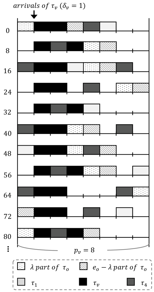
Figure 12: The schedule of the task set in Example 1 plotted on a schedule ladder diagram with a width of $p_{v}$. It shows that time columns $[1,3)$ are always occupied by either the victim task or other higher priority tasks. Therefore, the execution intervals of the observer task will not land on these time columns where the true arrival column is enclosed. This fact is what the proposed algorithms is based on.

References

- [1] M. Völp, C.-J. Hamann, and H. Härtig, “Avoiding timing channels in fixed-priority schedulers,” in Proceedings of the 2008 ACM Symposium on Information, Computer and Communications Security (ASIACCS), 2008, pp. 44–55.
- [2] A. Ghassami, X. Gong, and N. Kiyavash, “Capacity limit of queueing timing channel in shared fcfs schedulers,” in 2015 IEEE International Symposium on Information Theory (ISIT), June 2015, pp. 789–793.
- [3] J. Son and Alves-Foss, “Covert timing channel analysis of rate monotonic real-time scheduling algorithm in mls systems,” in 2006 IEEE Information Assurance Workshop, June 2006, pp. 361–368.
- [4] G. C. Buttazzo, Hard Real-Time Computing Systems: Predictable Scheduling Algorithms and Applications, 3rd ed. Springer Publishing Company, Incorporated, 2011.
- [5] C. L. Liu and J. W. Layland, “Scheduling algorithms for multiprogramming in a hard real-time environment,” Journal of the ACM, 1973.
- [6] J. Liu, Real-Time Systems. Prentice Hall, 2000.
- [7] C. Tankard, “Advanced persistent threats and how to monitor and deter them,” Network Security, vol. 2011, no. 8, pp. 16–19, 2011.
- [8] N. Virvilis and D. Gritzalis, “The big four - what we did wrong in advanced persistent threat detection?” in 2013 International Conference on Availability, Reliability and Security, Sep. 2013, pp. 248–254.
- [9] N. Falliere, L. O. Murchu, and E. Chien, “W32. stuxnet dossier,” White Paper, Symantec Corp., Security Response, vol. 5, no. 6, p. 29, 2011.
- [10] D. Isovic, Handling Sporadic Tasks in Real-time Systems: Combined Offline and Online Approach. Mälardalen University, 2001.
- [11] R. Pellizzoni, N. Paryab, M. Yoon, S. Bak, S. Mohan, and R. B. Bobba, “A generalized model for preventing information leakage in hard real-time systems,” in 21st IEEE Real-Time and Embedded Technology and Applications Symposium (RTAS), April 2015, pp. 271–282.
- [12] J.-S. Pleban, R. Band, and R. Creutzburg, “Hacking and securing the ar. drone 2.0 quadcopter: investigations for improving the security of a toy,” in IS&T/SPIE Electronic Imaging. International Society for Optics and Photonics, 2014, pp. 90 300L–90 300L.
- [13] F. Samland, J. Fruth, M. Hildebrandt, T. Hoppe, and J. Dittmann, “Ar. drone: security threat analysis and exemplary attack to track persons,” in Proceedings of The International Society for Optical Engineering (SPIE), vol. 8301, 2012.
- [14] The Linux Foundation. (2019, Jan.) The Real Time Linux Collaborative Project. [Online]. Available: https://wiki.linuxfoundation.org/realtime/
- [15] FreeRTOS. (2019, Jan.) The FreeRTOS Kernel. [Online]. Available: http://www.freertos.org/
- [16] jDrones. (2019, Jan.) ArduPilot Autopilot Suite. [Online]. Available: http://ardupilot.org/
- [17] D. A. Osvik, A. Shamir, and E. Tromer, “Cache attacks and countermeasures: the case of aes,” in Cryptographers’ Track at the RSA Conference. Springer, 2006, pp. 1–20.
- [18] D. Page, “Theoretical use of cache memory as a cryptanalytic side-channel.” IACR Cryptology ePrint Archive, vol. 2002, p. 169, 2002.
- [19] M. Yoon, S. Mohan, C. Chen, and L. Sha, “Taskshuffler: A schedule randomization protocol for obfuscation against timing inference attacks in real-time systems,” in 2016 IEEE Real-Time and Embedded Technology and Applications Symposium (RTAS), April 2016, pp. 1–12.
- [20] W.-M. Hu, “Lattice scheduling and covert channels,” in Research in Security and Privacy, Proceedings., IEEE, 1992.
- [21] J. Kelsey, B. Schneier, D. Wagner, and C. Hall, “Side channel cryptanalysis of product ciphers,” in European Symposium on Research in Computer Security, 1998.
- [22] Y. Zhang, A. Juels, M. K. Reiter, and T. Ristenpart, “Cross-vm side channels and their use to extract private keys,” in Proceedings of the 2012 ACM Conference on Computer and Communications Security (CCS), 2012, pp. 305–316.
- [23] G. Irazoqui, M. S. Inci, T. Eisenbarth, and B. Sunar, “Fine grain cross-vm attacks on xen and vmware,” in Big Data and Cloud Computing (BdCloud), IEEE, 2014.
- [24] T. Ristenpart, E. Tromer, H. Shacham, and S. Savage, “Hey, you, get off of my cloud: exploring information leakage in third-party compute clouds,” in Proceedings of the 16th ACM Conference on Computer and Communications Security (CCS), 2009, pp. 199–212.
- [25] Z. Wang and R. B. Lee, “New cache designs for thwarting software cache-based side channel attacks,” in Proceedings of the 34th Annual ACM International Symposium on Computer Architecture (ISCA), 2007, pp. 494–505.
- [26] K. Jiang, L. Batina, P. Eles, and Z. Peng, “Robustness analysis of real-time scheduling against differential power analysis attacks,” in 2014 IEEE Computer Society Annual Symposium on VLSI (ISVLSI), July 2014, pp. 450–455.
- [27] C. C. Tiu, “A new frequency-based side channel attack for embedded systems,” Tech. Rep., 2005.
- [28] D. Agrawal, B. Archambeault, J. R. Rao, and P. Rohatgi, “The em side-channel(s),” in the 4th International Workshop on Cryptographic Hardware and Embedded Systems, 2003.
- [29] M. Völp, B. Engel, C. Hamann, and H. Härtig, “On confidentiality-preserving real-time locking protocols,” in 2013 IEEE 19th Real-Time and Embedded Technology and Applications Symposium (RTAS), April 2013, pp. 153–162.
- [30] S. Kadloor, N. Kiyavash, and P. Venkitasubramaniam, “Mitigating timing side channel in shared schedulers,” IEEE/ACM Transactions on Networking, vol. 24, no. 3, pp. 1562–1573, June 2016.
- [31] X. Gong and N. Kiyavash, “Quantifying the information leakage in timing side channels in deterministic work-conserving schedulers,” IEEE/ACM Trans. Netw., vol. 24, no. 3, pp. 1841–1852, Jun. 2016.
- [32] S. Mohan, M. K. Yoon, R. Pellizzoni, and R. Bobba, “Real-time systems security through scheduler constraints,” in 2014 26th Euromicro Conference on Real-Time Systems (ECRTS), July 2014, pp. 129–140.
- [33] S. Mohan, S. Bak, E. Betti, H. Yun, L. Sha, and M. Caccamo, “S3A: Secure system simplex architecture for enhanced security and robustness of cyber-physical systems,” in Proceedings of the 2Nd ACM International Conference on High Confidence Networked Systems (HiCoNS), 2013, pp. 65–74.
- [34] M. Yoon, S. Mohan, J. Choi, J. Kim, and L. Sha, “SecureCore: A multicore-based intrusion detection architecture for real-time embedded systems,” in 2013 IEEE 19th Real-Time and Embedded Technology and Applications Symposium (RTAS), April 2013, pp. 21–32.
- [35] M. M. Z. Zadeh, M. Salem, N. Kumar, G. Cutulenco, and S. Fischmeister, “SiPTA: Signal processing for trace-based anomaly detection,” in Proceedings of the 14th International Conference on Embedded Software (EMSOFT), 2014, pp. 6:1–6:10.
- [36] M. Yoon, S. Mohan, J. Choi, and L. Sha, “Memory heat map: Anomaly detection in real-time embedded systems using memory behavior,” in 2015 52nd ACM/EDAC/IEEE Design Automation Conference (DAC), June 2015, pp. 1–6.
- [37] T. Xie and X. Qin, “Improving security for periodic tasks in embedded systems through scheduling,” ACM Transactions on Embedded Computing Systems (TECS), vol. 6, no. 3, Jul. 2007.
- [38] M. Lin, L. Xu, L. T. Yang, X. Qin, N. Zheng, Z. Wu, and M. Qiu, “Static security optimization for real-time systems,” IEEE Transactions on Industrial Informatics, vol. 5, no. 1, pp. 22–37, Feb 2009.
- [39] D. Trilla, C. Hernandez, J. Abella, and F. J. Cazorla, “Cache side-channel attacks and time-predictability in high-performance critical real-time systems,” in 2018 55th ACM/ESDA/IEEE Design Automation Conference (DAC), June 2018, pp. 1–6.
- [40] K. Krüger, M. Völp, and G. Fohler, “Vulnerability analysis and mitigation of directed timing inference based attacks on time-triggered systems,” in 30th Euromicro Conference on Real-Time Systems (ECRTS), 2018, pp. 22:1–22:17.