$\chi_{b}(3P)$ Multiplet Revisited: Ultrafine Mass Splitting and Radiative Transitions

Abstract

Invoked by the recent CMS observation regarding candidates of the $\chi_{b}(3P)$ multiplet, we analyze the ultrafine and mass splittings among $3P$ multiplet in our unquenched quark model (UQM) studies. The mass difference of $\chi_{b2}$ and $\chi_{b1}$ in $3P$ multiplet measured by CMS collaboration ($10.6\pm 0.64\pm 0.17$ MeV) is very close to our theoretical prediction ($12$ MeV). Our corresponding mass splitting of $\chi_{b1}$ and $\chi_{b0}$ enables us to predict more precisely the mass of $\chi_{b0}(3P)$ to be ($10490\pm 3$) MeV. Moreover, we predict ratios of the radiative decays of $\chi_{bJ}(nP)$ candidates, both in UQM and quark potential model. Our predicted relative branching fraction of $\chi_{b0}(3P)\to\Upsilon(3S)\gamma$ is one order of magnitude smaller than $\chi_{b2}(3P)$, this naturally explains the non-observation of $\chi_{b0}(3P)$ in recent CMS search. We hope these results might provide useful references for forthcoming experimental searches.

I Introduction

The excited $P$-wave bottomonia, $\chi_{bJ}(3P)$, are of special interest, since they provide a laboratory to test (and model) the non-perturbative spin-spin interactions of heavy quarks. Very recently, the CMS collaboration observed two candidates of the bottomonium $3P$ multiplet, $\chi_{b1}(3P)$ and $\chi_{b2}(3P)$, through their decays into $\Upsilon(3S)\gamma$ Sirunyan:2018dff . Their measured masses and mass splitting are

$$\begin{split}M[\chi_{b1}(3P)]=(10513.42\pm 0.41\pm 0.18)~{}\mathrm{MeV}~{},\\ M[\chi_{b2}(3P)]=(10524.02\pm 0.57\pm 0.18)~{}\mathrm{MeV}~{},\\ \Delta m_{21}\equiv m(\chi_{b2})-m(\chi_{b1})=(10.6\pm 0.64\pm 0.17)~{}\mathrm{MeV}~{}.\end{split}$$ (1)

There are some earlier measurements related to $\chi_{bJ}(3P)$ mass by ATLAS Aad:2011ih , LHCb Aaij:2014hla ; Aaij:2014caa , and D0 Collaborations Abazov:2012gh . However, these measurements can not distinguish between the candidates of $\chi_{bJ}(3P)$ multiplet. The recent CMS analysis Sirunyan:2018dff is higher resolution search, and hence, is able to distinguish between $\chi_{b1}(3P)$ and $\chi_{b2}(3P)$ for the first time.

In this paper we intend to compare our unquenched quark model studies with this recent measurement, and make more precise prediction for the mass of the other $3P$ bottomonium ($\chi_{b0}$) by incorporating the measured mass splitting. We also make an analysis of the ultrafine splitting of $P$-wave bottomonia, which enlighten the internal quark structure of the considered bottomonium. In addition, we predict model-independent ratios of radiative decays of $\chi_{bJ}(nP)$ candidates.

Heavy quarkonium states can couple to intermediate heavy mesons through the creation of light quark-antiquark pair which enlarge the Fock space of the initial state, i.e. the initial state contains multiquark components. These multiquark components will change the Hamiltonian of the potential model, causing the mass shift and mixing between states with the same quantum numbers or directly contributing to open channel strong decay if the initial state is above threshold. These can be summarized as coupled-channel effects (CCE). When CCE are combined with the naive quark potential model, one gets the unquenched quark model (UQM). UQM has been considered at least 35 years ago by Törnqvist et al. Heikkila:1983wd ; Ono:1983rd ; Ono:1985jt ; Ono:1985eu .

The physical or experimentally observed bottomonium state $\ket{A}$ is expressed in UQM as

$$\ket{A}=c_{0}\ket{\psi_{0}}+\sum_{BC}\int d^{3}p\,c_{BC}(p)\ket{BC;p},$$ (2)

where $c_{0}$ and $c_{BC}$ stand for the normalization constants of the bare state and the $BC$ components, respectively. In this work, $B$ and $C$ refer to bottom and anti-bottom mesons, and the summation over $BC$ is carried out including all possible pairs of ground-state bottom mesons. The $\ket{\psi_{0}}$ is normalized to 1 and $\ket{A}$ is also normalized to 1 if it lies below $B\bar{B}$ threshold, and $\ket{BC;p}$ is normalized as $\langle{BC;p_{1}}|{B^{\prime}C^{\prime};p_{2}}\rangle=\delta^{3}(p_{1}-p_{2})\delta_{BB^{\prime}}\delta_{CC^{\prime}}$, where $p$ is the momentum of $B$ meson in $\ket{A}$’s rest frame. The full Hamiltonian of the physical state then reads as

$$H=H_{0}+H_{BC}+H_{I},$$ (3)

where $H_{0}$ is the Hamiltonian of the bare state (see Appendix A for details), $H_{BC}\ket{BC;p}=E_{BC}\ket{BC;p}$ with $E_{BC}=\sqrt{m_{B}^{2}+p^{2}}+\sqrt{m_{C}^{2}+p^{2}}$ is the energy of the continuum state (interaction between $B$ and $C$ is neglected and the transition between one continuum to another is restricted), and $H_{I}$ is the interaction Hamiltonian which mix the bare state with the continuum. Since each quark pair creation model generates its own vertex functions that in turn lead to specific real parts of hadronic loops, see Ref. Hammer:2016prh for related remarks.

Here, for the bare-continuum mixing, we adopt the widely used ${}^{3}P_{0}$ model Micu:1968mk . In this model, the generated quark pairs have vacuum quantum numbers $J^{PC}=0^{++}$ which in spectroscopical notation ${}^{2S+1}L_{J}$ equals to ${}^{3}P_{0}$. A sketch of ${}^{3}P_{0}$ model induced mixing is shown in Fig. 1. The interaction Hamiltonian can be expressed as

$$H_{I}=2m_{q}\gamma\int d^{3}x\bar{\psi}_{q}\psi_{q},$$ (4)

where $m_{q}$ is the produced quark mass, and $\gamma$ is the dimensionless coupling constant. The $\psi_{q}$ ($\bar{\psi}_{q}$) is the spinor field to generate anti-quark (quark). Since the probability to generate heavier quarks is suppressed, we use the effective strength $\gamma_{s}=\frac{m_{q}}{m_{s}}\gamma$ in the following calculation, where $m_{q}=m_{u}=m_{d}$ is the constituent quark mass of up (or down) quark and $m_{s}$ is strange quark mass.

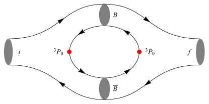
Figure 1: Sketch of coupled-channel effects in ${}^{3}P_{0}$ model. $i$ and $f$ respectively denote the initial and final states with same $J^{PC}$ and $B\bar{B}$ stands for all possible $B$ meson pairs.

The mass shift caused by the $BC$ components and the probabilities of the $b\bar{b}$ core are obtained after solving the Schrödinger equation with the full Hamiltonian $H$. They are expressed as

$$\Delta M :=M-M_{0}=\sum_{BC}\int d^{3}p\,\frac{|\bra{BC;p}H_{I}\ket{\psi_{0}}|^{2}}{M-E_{BC}-i\epsilon},$$ (5)

$$P_{b\bar{b}} :=|c_{0}|^{2}=\left(1+\sum_{BCLS}\int dp\frac{p^{2}\bra{BC;p}H_{I}\ket{\psi_{0}}|^{2}}{(M-E_{BC})^{2}}\right)^{-1},{}$$ (6)

where $M$ and $M_{0}$ are the eigenvalues of the full ($H$) and quenched/bare Hamiltonian ($H_{0}$), respectively. See Appendix B or Refs. Lu:2016mbb ; Ferretti:2013vua for derivation of above relations and UQM calculation details. Numerical values of $\Delta M$ and $P_{b\bar{b}}$ of every coupled channel for the bottomonia below $B\bar{B}$ threshold are given in Table 1, which will be used in the following discussions.

Initial States	$B\bar{B}$		$B\bar{B}^{*}+h.c.$		$B^{*}\bar{B}^{*}$		$B_{s}\bar{B}_{s}$		$B_{s}\bar{B}_{s}^{*}+h.c.$		$B_{s}^{*}\bar{B}^{*}_{s}$		Total
	$-\Delta M$	$P_{b\bar{b}}$	$-\Delta M$	$P_{b\bar{b}}$	$-\Delta M$	$P_{b\bar{b}}$	$-\Delta M$	$P_{b\bar{b}}$	$-\Delta M$	$P_{b\bar{b}}$	$-\Delta M$	$P_{b\bar{b}}$	$-\Delta M$	$P_{b\bar{b}}(\%)$
$\eta_{b}(1S)$	0	0	7.8	0.45	7.6	0.43	0	0	3.3	0.17	3.3	0.16	22.0	98.79
$\eta_{b}(2S)$	0	0	16.5	1.81	15.7	1.62	0	0	5.2	0.43	5.0	0.4	42.4	95.74
$\eta_{b}(3S)$	0	0	24.5	5.01	22.3	3.98	0	0	5.4	0.63	5.1	0.55	57.4	89.83
$\Upsilon(1S)$	1.4	0.09	5.4	0.33	9.2	0.54	0.6	0.03	2.3	0.12	3.9	0.2	22.8	98.69
$\Upsilon(2S)$	3.0	0.37	11.4	1.29	18.9	2.02	0.9	0.08	3.5	0.31	5.9	0.49	43.8	95.44
$\Upsilon(3S)$	4.8	1.25	17.2	3.71	27.1	5.07	1.0	0.13	3.7	0.45	6.1	0.67	60.0	88.71
$h_{b}(1P)$	0	0	13.5	1.22	13.0	1.12	0	0	4.8	0.35	4.6	0.33	35.8	96.99
$h_{b}(2P)$	0	0	21.9	3.51	20.3	2.96	0	0	5.6	0.59	5.3	0.52	53.1	92.43
$h_{b}(3P)$	0	0	38.0	19.75	29.5	9.04	0	0	5.4	0.67	5.0	0.54	77.9	70.0
$\chi_{b0}(1P)$	4.1	0.45	0	0	21.4	1.74	1.3	0.11	0	0	7.8	0.52	34.6	97.18
$\chi_{b0}(2P)$	9.3	1.85	0	0	31.1	4.13	2.1	0.26	0	0	8.4	0.77	50.9	92.98
$\chi_{b0}(3P)$	25.5	34.08	0	0	40.7	8.07	2.3	0.31	0	0	7.6	0.62	76.1	56.92
$\chi_{b1}(1P)$	0	0	10.8	1.03	15.5	1.27	0	0	3.7	0.28	5.6	0.38	35.5	97.03
$\chi_{b1}(2P)$	0	0	19.7	3.38	22.1	3.0	0	0	4.8	0.53	6.0	0.56	52.6	92.53
$\chi_{b1}(3P)$	0	0	37.4	21.9	29.7	7.54	0	0	4.8	0.64	5.4	0.54	77.4	69.38
$\chi_{b2}(1P)$	3.4	0.31	9.8	0.85	13.6	1.24	1.2	0.09	3.5	0.25	4.7	0.35	36.4	96.91
$\chi_{b2}(2P)$	5.3	0.89	14.6	2.23	23.2	3.62	1.3	0.15	3.8	0.39	5.8	0.6	54.1	92.13
$\chi_{b2}(3P)$	12.3	–	23.3	12.50	36.2	16.34	1.3	0.23	3.6	0.53	5.6	0.82	82.2	69.57

Table 1: The mass shift (in MeV) and probability (in %) of every coupled channel for the bottomonia below $B\bar{B}$ threshold. Note that since $h_{b}(3P)$ has no coupling to $B\bar{B}$, even though $h_{b}(3P)$ is above $B\bar{B}$ threshold, the probability is still well-defined. However, since $\chi_{b2}(3P)$ couples to $B\bar{B}$ channel and lies above this threshold, causing difficulty to the renormalization of the wave function. We make the assumption that the renormalization caused by $B\bar{B}$ channel can be discarded, see Sec. IV for related discussions.

II Mass Splitting and $\chi_{b0}(3P)$

After the recent CMS observation Sirunyan:2018dff of $\chi_{b1}(3P)$ and $\chi_{b2}(3P)$, $\chi_{b0}(3P)$ is now the only missing candidate in spin-triplet $3P$ bottomonium. With the reference of observed mass splitting of $1P$, $2P$ and $3P$ multiplets, one can predict the mass of $\chi_{b0}(3P)$. It requires a constraint that the mass splittings for $1P$, $2P$ and $3P$ multiplet should be the same Dib:2012vw .

Triggered by the above mentioned experimental search, we analyze our UQM studies regarding the bottomonium spectrum Lu:2016mbb ; Lu:2017hma . We notice that the measured mass splitting between $\chi_{b2}(3P)$ and $\chi_{b1}(3P)$ is $(10.6\pm 0.64\pm 0.17)$ MeV which differs only by $1$ MeV from our UQM prediction Lu:2016mbb . Our prediction for the mass splitting of $\chi_{b1}(3P)$ and $\chi_{b0}(3P)$ is $23$ MeV, see Table 2. With the reference of the observed masses of the other two candidates of spin-triplet $3P$ bottomonium, this mass splitting helps us to predict precisely the mass of unknown $\chi_{b0}(3P)$ to be

$$M[\chi_{b0}(3P)]=(10490\pm 3)~{}\mathrm{MeV}~{}.$$ (7)

The uncertainty in above prediction is calculated by taking the same percentage error [of $\mathcal{O}(10\%)$] in our mass splittings which we observed from CMS measurement. Our mass predictions respect the conventional pattern of splitting and support the standard mass hierarchy, where we have $M(\chi_{b2})>M(\chi_{b1})>M(\chi_{b0})$, which is in line with CMS measurement. A comparison of our UQM mass splittings with other quenched quark model predictions is given in Table 2.

Mass Splitting	Our UQM Lu:2016mbb	GI Godfrey:2015dia	Modified GI Wang:2018rjg	CQM Segovia:2016xqb	Exp Sirunyan:2018dff
$\chi_{b1}(3P)-\chi_{b0}(3P)$	$23$	$16$	$14$	$13$	$-$
$\chi_{b2}(3P)-\chi_{b1}(3P)$	$12$	$12$	$12$	$9$	$(10.6\pm 0.64\pm 0.17)$

Table 2: Mass splitting (in MeV) of $3P$-wave bottomonia in our UQM Lu:2016mbb , Godfrey-Isgur (GI) model Godfrey:2015dia , Modified GI model Wang:2018rjg , and constituent quark model (CQM) Segovia:2016xqb . The later three models are regarded as quenched quark models.

III Ultrafine Splitting in UQM

It is more informative if we study the mass splitting in a multiplet instead of the total mass shift caused by the intermediate meson loop. For the states quite below the threshold, there is an interesting phenomenon Burns:2011fu : the magnitude of the mass splitting is suppressed by the probability of the bottomonium core, $P_{b\bar{b}}$, if we turn on the meson loop.

There is also a pictorial explanation for this. Since under the potential model, the mass splitting $\delta M_{0}$ originates from the fine splitting Hamiltonian $H_{I}$. Up to the first order perturbation, we have $\delta M_{0}=\bra{\psi}H_{I}\ket{\psi}$, where $\psi$ is the two-body wave function in the quenched potential model. Since one of the coupled-channel effects is the wave function renormalization: $\bra{\psi}{\psi}\rangle=P_{b\bar{b}}<1$, one would simply expect that the $\delta M_{0}$ will be suppressed by this probability.

Moreover, due to the closeness of the spectrum of a multiplet, we expect that the $P_{b\bar{b}}$ of the states in a same multiplet are nearly the same, i.e., $\delta M_{0}$ are all suppressed by a same quantity, leaving the relation

$$\delta M_{P}\equiv\frac{1}{9}\Big{[}M(\chi_{b0})+3\cdot M(\chi_{b1})+5\cdot M(\chi_{b2})\Big{]}-M(h_{b})=0$$ (8)

intact, even if the coupled-channel effects are turned on. Due to the remarkably small $\delta M_{P}$, we refer it as “ultrafine splitting”. In our calculation, however, due to the finite size of the constituent quark, which is reflected by the smeared delta term, $\tilde{\delta}(r)$, instead of the true Dirac term in the spin dependent potential

$$V_{s}(r) =\frac{1}{m^{2}_{b}}\bigg{[}\left(\frac{2\alpha_{s}}{r^{3}}-\frac{\lambda}{2r}\right)\bm{\mathbf{L}}\cdot\bm{\mathbf{S}}+\frac{32\pi\alpha_{s}}{9}~{}\tilde{\delta}(r)~{}\bm{\mathbf{S}}_{b}\cdot\bm{\mathbf{S}}_{\bar{b}}$$

$$+\frac{4\alpha_{s}}{r^{3}}\left(\frac{\bm{\mathbf{S}}_{b}\cdot\bm{\mathbf{S}}_{\bar{b}}}{3}+\frac{(\bm{\mathbf{S}}_{b}\cdot\bm{\mathbf{r}})(\bm{\mathbf{S}}_{\bar{b}}\cdot\bm{\mathbf{r}})}{r^{2}}\right)\bigg{]}~{},$$ (9)

$$\tilde{\delta}(r) \equiv\bigg{(}\frac{\sigma}{\sqrt{\pi}}\bigg{)}^{3}e^{-\sigma^{2}r^{2}}~{},{}$$

where $\alpha_{s}$ and $\lambda$ are strengths of the color Coulomb and linear confinement potentials, respectively, and $\sigma$ is related to the width of Gaussian smeared function, the $\delta M_{P}$ relation of Eq. (8) is already violated a little bit under the potential model which can be seen from Table 3 (second column), where we also include the corresponding experimental values. We can also extract the threshold effects by taking the mass shift $\Delta M$ instead of $M$ in $\delta M_{P}$ calculations. The $\delta M_{P}$ values obtained in this way are also given in Table 3 (third column).

Multiplet	UQM prediction	CCE contribution	Experiment Patrignani:2016xqp
$1P$	$1.17$	$0.06$	$0.57(88)$
$2P$	$1.38$	$0.19$	$0.44(1.31)$
$3P$	$-0.39$	$2.08$	$-$

Table 3: Ultrafine splitting ($\delta M_{P}$ in MeV) for the $P$-wave bottomonia. The second to fourth columns are our unquenched quark model prediction, contribution from the coupled-channel effects and experimental results, respectively. The contribution from coupled-channel effects can be obtained by replacing the mass of $\chi_{bJ}(nP)$ by their mass shift $\Delta M$. Note that our results of $M_{0}$ violate Eq. (8) a bit due to finite size of the constituent quark, as discussed in the text.

We can see from Table 1 that although the mass shift for the $P$-wave multiplets is around 50 MeV, the modification of Eq. (8) is not very large, except $\delta M_{P}(3P)$ which is far larger than $\delta M_{P}(2P)$ and $\delta M_{P}(1P)$. A worth mentioning feature here is the hierarchy of these ultrafine splittings originated from the CCE (third column of Table 3), viz.,

$$\delta M_{P}(3P)>\delta M_{P}(2P)>\delta M_{P}(1P)~{},$$ (10)

which highlights that the coupled-channel effects bring meson masses closer together with respect to their bare values Burns:2011fu .

Channels	$\delta M_{0}$	$\widetilde{P}_{b\bar{b}}$	$(\widetilde{P}_{b\bar{b}}\times\delta M_{0})$	$\delta M$	$\widetilde{P}_{b\bar{b}}$	$(\widetilde{P}_{b\bar{b}}\times\delta M_{0})$	$\delta M$	$\delta M_{\text{Exp}}$
		GEM			SHO
$\Upsilon(1S)-\eta_{b}(1S)$	65.5	98.7	64.7	64.7	98.7	64.7	64.7	62.3
$\Upsilon(2S)-\eta_{b}(2S)$	30.7	95.5	29.3	29.4	95.9	29.4	29.5	24.3
$\Upsilon(3S)-\eta_{b}(3S)$	23.4	89.0	20.8	20.7	91.1	21.3	21.3	–
$\chi_{b0}(1P)-h_{b}(1P)$	-35.6	97.2	-34.6	-34.5	97.1	-34.6	-34.4	-39.9
$\chi_{b1}(1P)-h_{b}(1P)$	-6.3	97.0	-6.1	-6.0	97.0	-6.1	-6.0	-6.5
$\chi_{b2}(1P)-h_{b}(1P)$	13.2	96.9	12.8	12.6	96.8	12.8	12.7	12.9
$\chi_{b0}(2P)-h_{b}(2P)$	-31.2	93.0	-29.0	-28.9	93.4	-29.2	-29.1	-27.3
$\chi_{b1}(2P)-h_{b}(2P)$	-5.4	92.5	-5.0	-4.9	93.0	-5.0	-5.0	-4.3
$\chi_{b2}(2P)-h_{b}(2P)$	12.2	92.1	11.2	11.2	92.7	11.3	11.2	8.8
$\chi_{b0}(3P)-h_{b}(3P)$	-29.2	56.9	-16.6	-27.5	54.3	-15.8	-28.3	–
$\chi_{b1}(3P)-h_{b}(3P)$	-5.0	69.4	-3.5	-4.5	72.5	-3.6	-4.6	–
$\chi_{b2}(3P)-h_{b}(3P)$	11.9	–	–	7.5	–	–	7.7	–

Table 4: The mass splitting (in MeV) in a same $(n,L)$ multiplet, where $\delta M_{0}$, $\delta M$ and $\delta M_{\text{Exp}}$ represent the mass splitting in potential model, coupled-channel model and experiment, respectively. The $\widetilde{P}_{b\bar{b}}$ (in $\%$) is the weighted average of the probability, which for $P$- and $S$-wave is $\widetilde{P}_{b\bar{b}}=P_{b\bar{b}}(\chi_{bJ})$ and $\widetilde{P}_{b\bar{b}}=\frac{1}{4}P_{b\bar{b}}(\Upsilon)+\frac{3}{4}P_{b\bar{b}}(\eta_{b})$, respectively. The details of the mass splitting are given in Appendix C, and the absolute probabilities $P_{b\bar{b}}$ are given in Table 1. GEM and SHO stand for the Gaussian expansion method Hiyama:2003cu and simple harmonic oscillator approximation, respectively, to fit the numerical wave functions.

Since, for the $P$-wave states, no matter whether the threshold effects are considered or not, $h_{b}$ is not affected by the fine interaction, i.e. the $\delta M=0$. Hence, the $\chi_{bJ}$’s mass splitting are purely due to the $P_{b\bar{b}}$ of each $\chi_{bJ}$. Therefore, the weighted probability of the bottomonium core, $\widetilde{P}_{b\bar{b}}$, for $\chi_{bJ}(nP)$ multiplets is simply defined as $\widetilde{P}_{b\bar{b}}=P_{b\bar{b}}(\chi_{bJ})$. The weighted average probability for the $S$-wave bottomonia is discussed in Appendix C. From the Table 4, we can see that although the ($\widetilde{P}_{b\bar{b}}\times\delta M_{0}$) and $\delta M$ originate differently; one from the potential model and the other purely from the coupled-channel effects, but they are approximately equal to each other. The only large deviation comes from $\chi_{bJ}(3P)$.

As explained above, this overall suppression is based on the assumption that the $\widetilde{P}_{b\bar{b}}$ is the same (or approximately the same) for a multiplet. Indeed, from Table 1 we can see that this is quite reasonable assumption for the states which are far below the threshold. But for the $\chi_{b0}(3P)$, the $\widetilde{P}_{b\bar{b}}$ is quite different from that of $\chi_{b1}(3P)$, so this overall suppression does not make sense anymore. As a consequence, one should expect relatively large deviation from the $\delta M_{P}$ relation, as can be seen from $\delta M_{P}(3P)$ in Table 3.

The reason for this peculiar $\widetilde{P}_{b\bar{b}}$ is that even though the mass of $h_{b}(3P)$ and $\chi_{b1}(3P)$ is larger than the $\chi_{b0}(3P)$, they do not couple to the channel $B\bar{B}$, and the next open channel $B\bar{B}^{*}$ is somewhat farther from them. A net effect is that the $\widetilde{P}_{b\bar{b}}$ of $\chi_{b1}(3P)$ is larger than that of $\chi_{b0}(3P)$, breaking the $\widetilde{P}_{b\bar{b}}$ closeness assumption. This strong coupling of $\chi_{b0}(3P)$ to $B\bar{B}$ is also reflected by the large mass shift caused by $B\bar{B}$ which can be seen from Table 1. The observed mismatch between ($\widetilde{P}_{b\bar{b}}\times\delta M_{0}$) and $\delta M$ for $\chi_{bJ}(3P)$ multiplet is a smoking gun of the threshold effects which are beyond the quark potential model.

Recently, Lebed and Swanson also pointed out the remarkable importance of the $P$-wave heavy quarkonia Lebed:2017yme . For $1P$ and $2P$ charmonia, the ultrafine splitting is found to be astonishingly small. They argued that the ultrafine splitting can be used to delve the exoticness of the observed structure in the given multiplet Lebed:2017xih . According to their analysis Lebed:2017yme , the quantity $\delta M_{n,L=1,2,3,...}$ is found to be very small for any radial excitation $n$, both for the $b\bar{b}$ and $c\bar{c}$ sectors. The obtained constraint on the $\delta M_{n,L}$ value is

$$\delta M_{n,L=0,1,2,...}\ll\Lambda_{\textrm{QCD}}~{}.$$ (11)

This conclusion follows from several theoretical formalisms which do not consider coupled-channel effects or long-distance light-quark contributions in terms of intermediate meson-meson coupling to bare quarkonium states. As discussed above, the operators corresponding to ultrafine splitting involve spin-spin interactions which are suppressed by $1/m_{Q}^{2}$, the standard expansion parameter for the heavy quarkonium, where $m_{Q}$ is the mass of heavy quark. According to our point of view the above maxima is much large for the ultrafine splitting of $P$-wave bottomonia, see Table 3 for experimental corroboration. The more tight constraint could be

$$\delta M_{n,L=1,2,3,...}\lesssim\frac{\Lambda_{\textrm{QCD}}^{3}}{m_{Q}^{2}}~{}.$$ (12)

Since, quantitatively the $P$-wave excitation for the bottomonium is equal to $\Lambda_{\textrm{QCD}}$, which describes the emergence of the dynamical QCD scale in above relation. The $\delta M_{n,L}$ for the bottomonia with $L=1$ is expected to be of $\mathcal{O}(1~{}\mathrm{MeV})$, which can be verified from our analysis of Table 3.

The reason why $\delta M_{n,L=1,2,3,...}$ is exactly zero in the quark model is a consequence of the pure delta function nature of the $\bm{\mathbf{S}}_{b}\cdot\bm{\mathbf{S}}_{\bar{b}}$ term of Eq. (III), which is a perturbative one gluon exchange effect. The non-perturbative effects can make an additional contribution to this term, so that it is no longer a pure delta function. This give rise to introduce the smearing of the delta function in the quark models Barnes:2005pb ; Lebed:2017yme . However, one could use different non-perturbative forms for the spin-spin operator that contributes to the ultrafine splitting. For instance, the ultrafine splitting computed at next-to-next-to-next-to leading order (N³LO) Kiyo:2014uca in nonrelativistic QCD (NRQCD) Caswell:1985ui ; Brambilla:1999xf is

$$\delta M_{n,L=1}=\frac{m_{b}C^{4}_{F}\alpha^{5}_{s}}{432\pi(n+1)^{3}}(4n_{l}-N_{c})~{},$$ (13)

where $C_{F}$ is the color factor of bottomonium, $n_{l}$ being the number of light fermion species appearing in loop corrections, and $N_{c}$ is the number of colors in QCD. The computed $\delta M_{n,L=1}$ values using NRQCD for the bottomonium (with $m_{b}=4.5$ GeV and $\alpha_{s}(m_{b})=0.2$) are; $\delta M_{1P}=3.77$ keV, $\delta M_{2P}=1.12$ keV, and $\delta M_{3P}=0.47$ keV Lebed:2017yme . The remarkable smallness of these values strengthen the constraint on the $\delta M_{n,L=1,2,3,...}$ values presented in Eq. (12). However, these NRQCD predictions are much smaller as compared to our UQM predictions and corresponding experimental values, see Table 3. In conclusion, whatever the non-perturbative form for the spin-spin operator is used, the $\delta M_{n,L=1}$ should be very small, hence satisfying the relation of Eq. (12) quantitatively.

IV Radiative Transitions

Radiative transitions of higher bottomonia are of considerable interest, since they can shed light on their internal structure and provide one of the few pathways between different $b\bar{b}$ multiplets. Particularly, for those states which can not directly produce at $e^{+}e^{-}$ colliders (such as $P$-wave bottomonia), the radiative transitions serve as an elegant probe to explore such systems. In the quark model, the electric dipole ($E1$) transitions can be expressed as Kwong:1988ae ; Li:2009nr

$$\Gamma(n^{2S+1}L_{J}\to n^{\prime 2S^{\prime}+1}L^{\prime}_{J^{\prime}}+\gamma)=\frac{4}{3}C_{fi}\delta_{SS^{\prime}}e^{2}_{b}\alpha|\bra{\psi_{f}}r\ket{\psi_{i}}|^{2}E^{3}_{\gamma},$$ (14)

where $e_{b}=-\frac{1}{3}$ is the $b$-quark charge, $\alpha$ is the fine structure constant, and $E_{\gamma}$ denotes the energy of the emitted photon. The spatial matrix elements $\bra{\psi_{f}}r\ket{\psi_{i}}$ involve the initial and final radial wave functions, and $C_{fi}$ are the angular matrix elements. They are represented as

$$\bra{\psi_{f}}r\ket{\psi_{i}} = \int_{0}^{\infty}R_{f}(r)R_{i}(r)r^{3}dr,$$ (15)

$$C_{fi} = \max(L,L^{\prime})(2J^{\prime}+1)\left\{\begin{array}[]{ccc}L^{\prime}&J^{\prime}&S\\ J&L&1\end{array}\right\}^{2}.$$ (18)

The matrix elements $\bra{\psi_{f}}r\ket{\psi_{i}}$ are obtained numerically; for further details, we refer our studies Lu:2016mbb ; Lu:2017yhl . From Eq. (15), we know that the value of the decay width depends on the details of the wave functions, which are highly model dependent. A model independent prediction can be achieved by focusing on the following decay ratios

$$\Gamma\big{(}\chi_{bJ}(mP)\to\Upsilon(nS)+\gamma\big{)}\big{/}\Gamma\big{(}\chi_{b0}(mP)\to\Upsilon(nS)+\gamma\big{)}~{}.$$ (19)

Since, in the quark model, the spatial wave function is the same for the states in the same multiplet.

From the above discussion, we know that the meson loop renormalizes the bottomnium wave function. When the channel is above the corresponding open-bottom threshold (such as $B\bar{B}$ here), the wave function cannot be normalized to $1$, this is still an open problem (see e.g. Ref. Kalashnikova:2005ui ). On the other hand, the $B\bar{B}$ loop is still there, and have some CCE (such as mass renormalization). We make the assumption that for the states above threshold (such as $\chi_{b2}(3P)$ here), these open channels contribute equally to the wave functions of all $\chi_{bJ}(3P)$ states. In fact this is a reasonable assumption, since we can see this from the Table 1, the probability of $B\bar{B}$ is vanishingly small ($0.31\%$ and $0.89\%$, less than $1\%$) for both $\chi_{b0}(3P)$ and $\chi_{b1}(3P)$.

With the latest CMS data Sirunyan:2018dff and the $P_{b\bar{b}}$ in Table 1, our predictions of radiative decay ratios are listed in Table 5. From the Table 1, one can see that the small $P_{b\bar{b}}[\chi_{b0}(3P)]$ make the ratios in the last three rows notably larger than that of the potential model predictions, a peculiar feature of coupled-channel effects which can be tested in the upcoming experiments.

	Potential Model			Unquenched Quark Model
$\chi_{bJ}(1P)\to\Upsilon(1S)+\gamma$	1 :	3.80 :	7.20	1 :	3.79 :	7.18
$\chi_{bJ}(2P)\to\Upsilon(1S)+\gamma$	1 :	3.27 :	5.71	1 :	3.25 :	5.65
$\chi_{bJ}(2P)\to\Upsilon(2S)+\gamma$	1 :	4.09 :	8.02	1 :	4.07 :	7.95
$\chi_{bJ}(3P)\to\Upsilon(1S)+\gamma$	1 :	3.20 :	5.49	1 :	3.90 :	6.71
$\chi_{bJ}(3P)\to\Upsilon(2S)+\gamma$	1 :	3.46 :	6.15	1 :	4.22 :	7.51
$\chi_{bJ}(3P)\to\Upsilon(3S)+\gamma$	1 :	4.83 :	9.77	1 :	5.89 :	11.9

Table 5: Prediction for the ratios $\Gamma\big{(}\chi_{bJ}(mP)\to\Upsilon(nS)+\gamma\big{)}\big{/}\Gamma\big{(}\chi_{b0}(mP)\to\Upsilon(nS)+\gamma\big{)}$. For potential model calculations, the parameters and quenched Hamiltonian are same as Ref. Lu:2016mbb .

Another worth noting result from Table 5 is the relative size of the ratios for $\chi_{b0}(3P)$, which from the coupled-channel calculations is roughly $1:6:12$. This reflects that the $\chi_{b0}(3P)$ has negligible radiative decay branching fraction with comparison to $\chi_{b1}(3P)$ and $\chi_{b2}(3P)$. Compared with the potential model, the suppression of the $\chi_{b0}(3P)$’s radiative width in the UQM is more consistent with the non-observation of the $\chi_{b0}(3P)$ in the recent CMS search of $\chi_{bJ}(3P)\to\Upsilon(3S)\gamma$ Sirunyan:2018dff . This indicates that our UQM predictions are more reliable than the naive quark potential models.

V Conclusions

The recent CMS study successfully distinguishs $\chi_{b1}(3P)$ and $\chi_{b2}(3P)$ for the first time, and measures their mass splitting which differs only $1$ MeV from our unquenched quark model predictions. This measurement gives us confidence to predict mass of the lowest candidate of $3P$ multiplet to be $M[\chi_{b0}(3P)]=(10490\pm 3)~{}\mathrm{MeV}$, based on our unquenched quark model results of the mass splittings of this multiplet. We also analyze the ultrafine splittings of $P$-wave bottomonia up to $n=3$ in the framework of UQM, and put a constraint on them based on recent experimental corroboration. No matter which non-perturbative form for the spin-spin operator is used, the ultrafine splitting for the $P$-wave bottomonia should be very small. This analysis leads us to conclude that the coupled-channel effects play a crucial role to understand the higher bottomonia close to open-flavor thresholds.

At last, we predict here to some extent model-independent ratios of the radiative decays of $\chi_{bJ}(nP)$ candidates. A worth mentioning observation is that the coupled-channel effects can enhance the radiative decay ratios of $\chi_{bJ}(3P)$ as compared to the naive potential model predictions. The relative branching fraction of $\chi_{b0}(3P)\to\Upsilon(3S)\gamma$ is negligible as compared to the other candidates of this multiplet, which naturally explains its non-observation in recent CMS search.

We hope above highlighted features of coupled-channel model provide useful references for the understanding of higher $P$-wave bottomonia and can be explored in ongoing and future experiments.

Appendix A Bare Hamiltonian

Bare states are obtained by solving the Schrödinger equation with the well-known Cornell potential Eichten:1978tg ; Eichten:1979ms , which incorporates a spin-independent color Coulomb plus linear confined (scalar) potential. In the quenched limit, the potential can be written as

$$V(r)=-\frac{4}{3}\frac{\alpha}{r}+\lambda r+c,$$ (20)

where $\alpha,\lambda$ and $c$ stand for the strength of color Coulomb potential, the strength of linear confinement and mass renormalization, respectively. The hyperfine and fine structures are generated by the spin dependent interactions

$$V_{s}(r) =\frac{1}{m^{2}_{b}}\bigg{[}\left(\frac{2\alpha_{s}}{r^{3}}-\frac{\lambda}{2r}\right)\bm{\mathbf{L}}\cdot\bm{\mathbf{S}}+\frac{32\pi\alpha_{s}}{9}~{}\tilde{\delta}(r)~{}\bm{\mathbf{S}}_{b}\cdot\bm{\mathbf{S}}_{\bar{b}}$$ (21)

$$+\frac{4\alpha_{s}}{r^{3}}\left(\frac{\bm{\mathbf{S}}_{b}\cdot\bm{\mathbf{S}}_{\bar{b}}}{3}+\frac{(\bm{\mathbf{S}}_{b}\cdot\bm{\mathbf{r}})(\bm{\mathbf{S}}_{\bar{b}}\cdot\bm{\mathbf{r}})}{r^{2}}\right)\bigg{]}~{},{}$$

where $\bm{\mathbf{L}}$ denotes the relative orbital angular momentum, $\bm{\mathbf{S}}=\bm{\mathbf{S}}_{b}+\bm{\mathbf{S}}_{\bar{b}}$ is the total spin of the charm quark pairs and $m_{b}$ is the bottom quark mass. The smeared $\tilde{\delta}(r)$ function can be read from Eq. (III) or Refs. Barnes:2005pb ; Li:2009ad . These spin dependent terms are treated as perturbations.

The Hamiltonian of the Schrödinger equation in the quenched limit is represented as

$$H_{0}=2m_{b}+\frac{p^{2}}{m_{b}}+V(r)+V_{s}(r).$$ (22)

The spatial wave functions and bare mass $M_{0}$ are obtained by solving the Schrödinger equation numerically using the Numerov method Numerov:1927 . The full bare-mass spectrum is given in Ref. Lu:2016mbb .

Appendix B Details of the Coupled-Channel Effects

As sketched by Fig. 1, the experimentally observed state should be a mixture of pure quarkonium state (bare state) and $B$ meson continuum. The coupled-channel effects can be deduced by following way

$$H_{0}\ket{\psi_{0}} = M_{0}\ket{\psi_{0}}$$ (23)

$$H_{0}\ket{BC;p} = 0$$ (24)

$$H_{BC}\ket{\psi_{0}} = 0$$ (25)

$$H_{BC}\ket{BC;p} = E_{BC}\ket{BC;p}$$ (26)

$$H\ket{A} = M\ket{A},$$ (27)

where $M_{0}$ is the bare mass of the bottomonium and can be solved directly from Schrödinger equation, and $M$ is the physical mass. The interaction between $B$ mesons is neglected. When Eq. (27) is projected onto each component, we immediately get

$$\bra{\psi_{0}}H\ket{\psi}=c_{0}M=c_{0}M_{0}+\int d^{3}p\,c_{BC}(p)\bra{\psi_{0}}H_{I}\ket{BC;p},$$ (28)

$$\bra{BC;p}H\ket{\psi}=c_{BC}(p)M=c_{BC}(p)E_{BC}+c_{0}\bra{BC;p}H_{I}\ket{\psi_{0}}.$$ (29)

Solve $c_{BC}$ from Eq. (29), substitute back to Eq. (28) and eliminate the $c_{0}$ on both sides, we get a integral equation

$$M=M_{0}+\Delta M,$$ (30)

where $\Delta M$ is given in Eq. (5). Once $M$ is solved, the coefficient of different components can be worked out either. For states below threshold, the normalization condition $\ket{A}$ can be rewritten as

$$|c_{0}|^{2}+\int d^{3}p|c_{BC}|^{2}=1$$ (31)

after the substitution of $c_{BC}$, we get the probability of the $b\bar{b}$ component. The sum of $BC$ is restricted to the ground state $B_{(s)}$ mesons, i.e. $B\bar{B},B\bar{B}^{*}+h.c.,B^{*}\bar{B}^{*},B_{s}\bar{B}_{s},B_{s}\bar{B}^{*}_{s}+h.c.,B^{*}_{s}\bar{B}^{*}_{s}$.

The coupled-channel effects calculation cannot proceed if the wave functions of the $\ket{\psi_{0}}$ and $BC$ components are not settled in Eq.(7). Since the major part of the coupled-channel effects calculation is encoded in the wave function overlap integration,

$$\bra{BC;p}H_{I}\ket{\psi_{0}} =\int d^{3}k\phi_{0}(\vec{k}+\vec{p})\phi_{B}^{*}(\vec{k}+x\vec{p})\phi_{C}^{*}(\vec{k}+x\vec{p})$$

$$~{}~{}~{}~{}\times|\vec{k}|Y_{1}^{m}(\theta_{\vec{k}},\phi_{\vec{k}})~{},{}$$ (32)

where $x=m_{q}/(m_{Q}+m_{q})$, and $m_{Q}$ and $m_{q}$ denote the bottom quark and the light quark mass, respectively. The $\phi_{0},\phi_{B}$ and $\phi_{C}$ are the wave functions of $\ket{\psi_{0}}$ and $BC$ components, respectively and the notation $*$ stands for the complex conjugate. These wave functions are in momentum space, and they are obtained by the Fourier transformation of the eigenfunctions of the bare Hamiltonian $H_{0}$. More details can be found in our earlier works Lu:2016mbb ; Lu:2017yhl .

Appendix C Ultrafine Mass Splitting for $S$-Wave Bottomonia

For the $S$-wave ($\eta_{b}$ and $\Upsilon$) bottomonia, we define

$$\delta M_{S}\equiv\frac{32\pi\alpha}{9m_{b}^{2}}|R(0)|^{2}$$ (33)

Due to the $\bm{\mathbf{S}}\cdot\bm{\mathbf{S}}$ interaction term in Eq. (III), we have $\delta M_{0}$:

$$\delta M_{0}(\eta_{b}) =-\frac{3}{4}\delta M_{S}~{},$$

$$\delta M_{0}(\Upsilon) =+\frac{1}{4}\delta M_{S}~{}.{}$$ (34)

After the suppression of $P_{b\bar{b}}({\eta_{b}})$ and $P_{b\bar{b}}({\Upsilon})$, the mass splitting becomes,

$$M(\Upsilon)-M(\eta_{b})\equiv\delta M(\Upsilon)-\delta M(\eta_{b})=\bigg{(}\frac{1}{4}P_{b\bar{b}}(\Upsilon)+\frac{3}{4}P_{b\bar{b}}(\eta_{b})\bigg{)}~{}\delta M_{S}~{}.$$ (35)

So for the $S$-wave bottomonium, we defined the weighted average of the $P_{b\bar{b}}$

$$\widetilde{P}_{b\bar{b}}=\frac{1}{4}P_{b\bar{b}}(\Upsilon)+\frac{3}{4}P_{b\bar{b}}(\eta_{b})~{}.$$ (36)

References

- (1) A. M. Sirunyan et al. [CMS Collaboration], “Observation of the (3P) and (3P) and measurement of their masses,” Phys. Rev. Lett. 121, 092002 (2018).
- (2) G. Aad et al. [ATLAS Collaboration], “Observation of a new state in radiative transitions to and at ATLAS,” Phys. Rev. Lett. 108, 152001 (2012).
- (3) R. Aaij et al. [LHCb Collaboration], “Measurement of the mass and of the relative rate of and production,” JHEP 1410, 088 (2014).
- (4) R. Aaij et al. [LHCb Collaboration], “Study of meson production in collisions at and and observation of the decay ,” Eur. Phys. J. C 74, 3092 (2014).
- (5) V. M. Abazov et al. [D0 Collaboration], “Observation of a narrow mass state decaying into in collisions at TeV,” Phys. Rev. D 86, 031103 (2012).
- (6) K. Heikkila, S. Ono and N. A. Tornqvist, “HEAVY c anti-c AND b anti-b QUARKONIUM STATES AND UNITARITY EFFECTS,” Phys. Rev. D 29, 110 (1984).
- (7) S. Ono and N. A. Tornqvist, “Continuum Mixing and Coupled Channel Effects in and Quarkonium,” Z. Phys. C 23, 59 (1984).
- (8) S. Ono, A. I. Sanda, N. A. Tornqvist and J. Lee-Franzini, “Where Are the Mixing Effects Observable in the Region?,” Phys. Rev. Lett. 55, 2938 (1985).
- (9) S. Ono, A. I. Sanda and N. A. Tornqvist, “ Meson Production Between the (4s) and (6s) and the Possibility of Detecting Mixing,” Phys. Rev. D 34, 186 (1986).
- (10) I. K. Hammer, C. Hanhart and A. V. Nefediev, “Remarks on meson loop effects on quark models,” Eur. Phys. J. A 52, 330 (2016).
- (11) L. Micu, “Decay rates of meson resonances in a quark model,” Nucl. Phys. B 10, 521 (1969).
- (12) Y. Lu, M. N. Anwar and B. S. Zou, “Coupled-Channel Effects for the Bottomonium with Realistic Wave Functions,” Phys. Rev. D 94, 034021 (2016).
- (13) J. Ferretti and E. Santopinto, “Higher mass bottomonia,” Phys. Rev. D 90, 094022 (2014); “Threshold corrections of and states and and transitions of the in a coupled-channel model,” Phys. Lett. B 789, 550 (2019).
- (14) C. O. Dib and N. Neill, “ splitting predictions in potential models,” Phys. Rev. D 86, 094011 (2012).
- (15) Y. Lu, M. N. Anwar and B. S. Zou, “How Large is the Contribution of Excited Mesons in Coupled-Channel Effects?,” Phys. Rev. D 95, 034018 (2017).
- (16) T. J. Burns, “How the small hyperfine splitting of P-wave mesons evades large loop corrections,” Phys. Rev. D 84, 034021 (2011); “P-Wave Spin-Spin Splitting and Meson Loops,” in Proceedings, 14th International Conference on Hadron spectroscopy (Hadron 2011): Munich, Germany, June 13-17, 2011, arXiv:1108.5259 [hep-ph].
- (17) T. Barnes, S. Godfrey and E. S. Swanson, “Higher charmonia,” Phys. Rev. D 72, 054026 (2005).
- (18) S. Godfrey and K. Moats, “Bottomonium Mesons and Strategies for their Observation,” Phys. Rev. D 92, 054034 (2015).
- (19) J. Z. Wang, Z. F. Sun, X. Liu and T. Matsuki, “Higher bottomonium zoo,” Eur. Phys. J. C 78, 915 (2018).
- (20) J. Segovia, P. G. Ortega, D. R. Entem and F. Fernandez, “Bottomonium spectrum revisited,” Phys. Rev. D 93, 074027 (2016).
- (21) C. Patrignani et al. [Particle Data Group], “Review of Particle Physics,” Chin. Phys. C 40, 100001 (2016).
- (22) R. F. Lebed and E. S. Swanson, “Quarkonium States As Arbiters of Exoticity,” Phys. Rev. D 96, 056015 (2017).
- (23) R. F. Lebed and E. S. Swanson, “Heavy-Quark Hybrid Mass Splittings: Hyperfine and ”Ultrafine”,” Few Body Syst. 59, 53 (2018).
- (24) Y. Kiyo and Y. Sumino, “Full Formula for Heavy Quarkonium Energy Levels at Next-to-next-to-next-to-leading Order,” Nucl. Phys. B 889, 156 (2014); “Perturbative heavy quarkonium spectrum at next-to-next-to-next-to-leading order,” Phys. Lett. B 730, 76 (2014).
- (25) W. E. Caswell and G. P. Lepage, “Effective Lagrangians for Bound State Problems in QED, QCD, and Other Field Theories,” Phys. Lett. 167B, 437 (1986).
- (26) N. Brambilla, A. Pineda, J. Soto and A. Vairo, “Potential NRQCD: An Effective theory for heavy quarkonium,” Nucl. Phys. B 566, 275 (2000).
- (27) E. Hiyama, Y. Kino and M. Kamimura, “Gaussian expansion method for few-body systems,” Prog. Part. Nucl. Phys. 51, 223 (2003).
- (28) W. Kwong and J. L. Rosner, “ Wave Quarkonium Levels of the Family,” Phys. Rev. D 38, 279 (1988).
- (29) B. Q. Li and K. T. Chao, “Bottomonium Spectrum with Screened Potential,” Commun. Theor. Phys. 52, 653 (2009)
- (30) Y. Lu, M. N. Anwar and B. S. Zou, “ Revisited: A Coupled Channel Perspective,” Phys. Rev. D 96, 114022 (2017).
- (31) Y. S. Kalashnikova, “Coupled-channel model for charmonium levels and an option for X(3872),” Phys. Rev. D 72, 034010 (2005).
- (32) E. Eichten, K. Gottfried, T. Kinoshita, K. D. Lane and T. M. Yan, “Charmonium: The Model,” Phys. Rev. D 17, 3090 (1978); 21, 313 (E) (1980); “Charmonium: Comparison with Experiment,” Phys. Rev. D 21, 203 (1980).
- (33) E. Eichten, K. Gottfried, T. Kinoshita, K. D. Lane and T. M. Yan, “Charmonium: Comparison with Experiment,” Phys. Rev. D 21, 203 (1980).
- (34) B. Q. Li, C. Meng and K. T. Chao, “Coupled-Channel and Screening Effects in Charmonium Spectrum,” Phys. Rev. D 80, 014012 (2009).
- (35) B. Numerov, “Note on the numerical integration of ,” Astron. Nachr. 230, 359 (1927).