The methane distribution and polar brightening on Uranus based on HST/STIS, Keck/NIRC2, and IRTF/SpeX observations through 2015

Abstract

Space Telescope Imaging Spectrograph (STIS) observations of Uranus in 2015 show that the depletion of upper tropospheric methane has been relatively stable and that the polar region has been brightening over time as a result of increased aerosol scattering. This interpretation is confirmed by near-IR imaging from HST and from the Keck telescope using NIRC2 adaptive optics imaging. Our analysis of the 2015 spectra, as well as prior spectra from 2012, shows that there is a factor of three decrease in the effective upper tropospheric methane mixing ratio between 30^∘ N and 70^∘ N. The absolute value of the deep methane mixing ratio, which probably does not vary with latitude, is lower than our previous estimate, and depends significantly on the style of aerosol model that we assume, ranging from a high of 3.5$\pm$0.5% for conservative non-spherical particles with a simple Henyey-Greenstein phase function to a low of 2.7%$\pm$0.3% for conservative spherical particles. Our previous higher estimate of 4$\pm$0.5% was a result of a forced consistency with occultation results of Lindal et al. (1987, JGR 92, 14987-15001). That requirement was abandoned in our new analysis because new work by Orton et al. (2014, Icarus 243, 494-513) and by Lellouch et al. (2015, Astron. & AstroPhys. 579, A121), called into question the occultation results. For the main cloud layer in our models we found that both large and small particle solutions are possible for spherical particle models. At low latitudes the small-particle solution has a mean particle radius near 0.3 $\mu$m, a real refractive index near 1.65, and a total column mass of 0.03 mg/cm², while the large-particle solution has a particle radius near 1.5 $\mu$m, a real index near 1.24, and a total column mass 30 times larger. The pressure boundaries of the main cloud layer are between about 1.1 and 3 bars, within which H₂S is the most plausible condensable.

1. Introduction

The visible and infrared spectra of Uranus are both dominated by the absorption features of methane, its third most abundant gas. In some spectral regions, however, the effects of collision-induced absorption (CIA) by hydrogen can be seen competing with methane. Those wavelengths provide constraints on the number density of methane with respect to hydrogen, and thus on the volume mixing ratio of methane. From analysis of HST/STIS spatially resolved spectra of Uranus obtained in 2002, 5 years before equinox and limited to latitudes south of 30^∘ N, Karkoschka and Tomasko (2009), henceforth referred to as KT2009, discovered that good fits to the latitudinal variation of these spectra required a latitudinal variation in the effective volume mixing ratio of methane. They inferred that the southern polar region was depleted in methane with respect to low latitudes by about a factor of two. This suggested a possible meridional circulation in which upwelling methane-rich gas at low latitudes was dried out by condensation then moved to high latitudes, where descending motions brought the methane-depleted gas downward, with a return flow at deeper levels.

Because post equinox groundbased observations revealed numerous small “convective” features in the north polar region that had not been seen in the south polar region just prior to equinox, Sromovsky et al. (2012b) suggested that the downwelling movement of methane-depleted gas would suppress convection in the south polar region, providing a plausible explanation for the lack of discrete cloud features there, and further suggested that the presence of discrete cloud features at high northern latitudes might mean that methane is not depleted there. However, using 2012 HST/STIS observations designed to test that hypothesis, Sromovsky et al. (2014) showed that the depletion was indeed symmetric, with both polar regions depleted by similar amounts, and from imaging observations taken near equinox using discrete narrow band filters that sampled methane-dominated and hydrogen-dominated wavelengths, they showed that the symmetry was also present at equinox and thus probably a stable feature of the Uranian atmosphere.

In spite of the apparent general stability of the latitudinal distribution of methane, there were significant post-equinox increases in the brightness of the north polar region, as well as some evidence for brightening at low latitudes. New HST/STIS observations were obtained in 2015 to further investigate possible changes in the methane distribution and the nature of the polar brightening that was taking place.

Other relevant developments occurred since our last analysis of the HST/STIS spectra of Uranus. The first is the inference of new mean temperature and methane profiles for Uranus by Orton et al. (2014a), which are in disagreement with the occultation-based profiles of Lindal et al. (1987) and also with those using a reduced He/H₂ volume mixing ratio derived by Sromovsky et al. (2011). The second development is an independent determination of the methane volume mixing ratio in the lower stratosphere and upper troposphere by Lellouch et al. (2015) using Herschel far infrared and sub-mm observations. Since both of these results question the validity of Uranus occultation results in general, and more specifically the validity of using them at all times and all latitudes, we decided to modify our analysis so that models would be constrained by STIS spectral observations alone, and abandoned the requirement that our low-latitude methane profiles also be consistent with occultation constraints. We also took a fresh look at how to best model the aerosol structure, and found that a much simpler 2-3 layer structure could produce fits as accurate as the more complex five-layer structure we had used in our previous analysis of the 2012 STIS observations.

In the following we first describe the approach to constraining the methane mixing ratio on Uranus, then discuss the new thermal profile for Uranus and its implications. We follow that with a discussion of our STIS, WFC3, and Keck supporting observations, the calibration of the STIS spectra, direct comparisons of STIS spectra, comparisons of imaging observations at key wavelengths, description of our approach to radiative transfer modeling, results of modeling cloud structure and the distribution of methane, interpretation of those results, how models can be extended to longer wavelengths to match spectra obtained at NASA’s Infrared Telescope Facility (IRTF), comparisons with other models, and a final summary and conclusions.

2. How observations constrain the methane mixing ratio on Uranus

Constraining the mixing ratio of CH₄ on Uranus is based on differences in the spectral absorption of CH₄ and H₂, illustrated by the penetration depth plot of Fig. 1. There methane absorption can be seen to dominate at most wavelengths, while hydrogen’s Collision Induced Absorption (CIA) is relatively more important in narrow spectral ranges near 825 nm, which is covered by our STIS observations, and also near 1080 nm, which we were able to sample with imaging observations using the NICMOS F108N filter and Keck He1_A filter. Model calculations that don’t have the correct ratio of methane to hydrogen lead to a relative reflectivity mismatch near these wavelengths. Karkoschka and Tomasko (2009) used the 825-nm spectral constraint to infer a methane mixing ratio of 3.2% at low latitudes, but dropping to 1.4% at high southern latitudes. Sromovsky et al. (2011) analyzed the same data set, but used only temperature and mixing ratio profiles that were consistent with the Lindal et al. (1987) refractivity profiles. They confirmed the depletion but inferred a somewhat higher mixing ratio of 4% at low latitudes and found that better fits were obtained if the high latitude depletion was restricted to the upper troposphere (down to $\sim$2-4 bars). Subsequently, 2009 groundbased spectral observations at the NASA Infrared Telescope Facility (IRTF) using the SpeX instrument, which provided coverage of the key 825-nm spectral region, were used by Tice et al. (2013) to infer that both northern and southern mid latitudes were weakly depleted in methane, relative to the near equatorial region, which was enriched by at least 9%. Their I-band analysis yielded a broad peak centered at 6^∘S, which was 32$\pm$24% above the minimum found at 44^∘N. These low IRTF-based values for the latitudinal variation might be partly a result of lower spatial resolution combined with worse view angles into higher latitudes than obtained by HST observations.

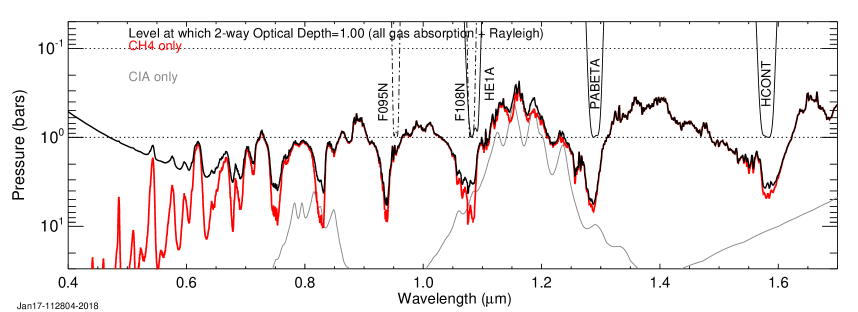
Figure 1.— Penetration depth vs. wavelength as limited by different opacity sources assuming the Orton et al. (2014a) temperature profile and a 3.5% deep methane mixing ratio. Where absorption dominates, penetration is about one optical depth, but when Rayleigh scattering dominates, light can penetrate many optical depths. Transmission profiles of key HST/NICMOS (dot-dash) and Keck NIRC2 (solid) narrow-band filters are also plotted.

3. HST/STIS 2015 Observations

Our 2015 spectral observations of Uranus (Cycle 23 HST program 14113, L. Sromovsky P.I.) used four HST orbits, three of them devoted to STIS spatial mosaics and one devoted to Wide Field Camera 3 (WFC3) support imaging. The STIS observations were taken on 10 October 2015 and the WFC3 observations on 11 October 2015. Observing conditions and exposures are summarized in Table 1.

Table 1Science exposures from 2015 HST program 14113.

Relative	Start	Start	Instrument	Filter or	Exposure	No. of	Phase
Orbit	Date (UT)	Time (UT)		Grating	(sec)	Exp.	Angle (∘)
1	2015-10-10	13:54:06	STIS	MIRVIS	5.0	1	0.09
1	2015-10-10	14:09:48	STIS	G430L	70.0	13	0.09
2	2015-10-10	15:28:02	STIS	G750L	84.0	19	0.09
3	2015-10-10	17:03:25	STIS	G750L	84.0	19	0.09
19	2015-10-11	18:30:59	WFC3	F336W	30.0	1	0.04
19	2015-10-11	18:32:44	WFC3	F467M	16.0	1	0.04
19	2015-10-11	18:34:24	WFC3	F547M	6.0	1	0.04
19	2015-10-11	18:35:48	WFC3	F631N	65.0	1	0.04
19	2015-10-11	18:38:17	WFC3	F665N	52.0	1	0.04
19	2015-10-11	18:40:24	WFC3	F763M	26.0	1	0.04
19	2015-10-11	18:42:11	WFC3	F845M	35.0	1	0.04
19	2015-10-11	18:44:05	WFC3	F953N	250.0	1	0.04
19	2015-10-11	18:50:43	WFC3	FQ889N	450.0	1	0.04
19	2015-10-11	19:02:25	WFC3	FQ937N	150.0	1	0.04
19	2015-10-11	19:09:25	WFC3	FQ727N	210.0	1	0.04

On October 10 the sub-observer planetographic latitude was 31.7^∘ S, the observer range was 18.984 AU (2.8400$\times$10⁹ km), and the equatorial angular diameter of Uranus was 3.7126 arcseconds. The first two STIS orbits used the 52${}^{\prime\prime}\times$0.1^′′ slit and the third inadvertently used the 52${}^{\prime\prime}\times$0.05^′′ slit

3.1. STIS spatial mosaics.

Our STIS observations used the G430L and G750L gratings and the CCD detector, which has $\sim$0.05 arcsecond square pixels covering a nominal 52${}^{\prime\prime}\times$52^′′ square field of view (FOV) and a spectral range from $\sim$200 to 1030 nm (Hernandez et al., 2012). Using the 52${}^{\prime\prime}\times$0.1^′′ slit, the resolving power varies from 500 to 1000 over each wavelength range due to fixed wavelength dispersion of the gratings. Observations had to be carried out within a few days of Uranus opposition (12 October 2015) when the telescope roll angle could be set to orient the STIS slit parallel to the spin axis of Uranus.

One STIS orbit produced a mosaic of half of Uranus using the CCD detector, the G430L grating, and the 52${}^{\prime\prime}\times$0.1^′′ slit. The G430L grating covers 290 to 570 nm with a 0.273 nm/pixel dispersion. The slit was aligned with Uranus’ rotational axis, and stepped from the evening limb to the central meridian in 0.152 arcsecond increments (because the planet has no high spatial resolution center-to-limb features at these wavelengths we used interpolation to fill in missing columns of the mosaic). Two additional STIS orbits were used to mosaic the planet with the G750L grating. We intended to use the 52${}^{\prime\prime}\times$0.1^′′ slit (524-1027 nm coverage with 0.492 nm/pixel dispersion) for both orbits, but an error in the program resulted in half of the half-disk covered with the nominal 0.05^′′ slit. This produced a higher spectral resolution at the cost of a significant reduction in signal to noise ratio. The limb to central meridian stepping was at 0.0562 arcsecond intervals for the G750L grating. Aside from the slit width error, this was the same procedure that was used successfully for HST program 9035 in 2002 (E. Karkoschka, P.I.) and for HST program 12894 in 2012 (L. Sromovsky, P.I.). As Uranus’ equatorial radius was 1.85 arcseconds when observations were performed, stepping from one step off the limb to the central meridian required 13 positions for the G430L grating and 36 for the G750L grating. Two orbits were needed to complete the G750L grating observations, spanning a total time of 2 h 17 m, during which Uranus rotated 47^∘. This rotation was not a problem because of the high degree of zonal symmetry of Uranus and because our analysis rejected any small scale deviations from it.

Exposure times were similar to those used in the 2002 and 2012 programs, with 70-second exposures for G430L and 84-second exposures for G750L gratings, using the 1 electron/DN gain setting. These exposures yielded single-pixel signal-to-noise ratios of around 10:1 at 300 nm, $>$ 40:1 from around 400 to 700 nm, and decreasing to around 20:1 (methane windows) to $<$ 10:1 (methane absorption bands) at 1000 nm. For the G750L grating, the part of the planet covered by the narrow slit setting (from 0.9^′′ from the planet center to the central meridian) the signal to noise at continuum wavelengths was reduced by a factor of $\sim$1.7 at short wavelengths to $\sim$2.1 at the longest wavelengths. In methane bands, where readout noise dominates, the degradation factor was $\sim$4.5.

3.2. Supporting WFC3 imaging.

The complex radiometric calibration of the STIS spectra relies on calibrated WFC3 images to provide the final wavelength dependent correction functions. To ensure that this function was determined as well as possible for the Cycle 23 observations in 2015, and to cross check the extensive spatial and spectral corrections that are required for STIS observations, we used one additional orbit of WFC3 imaging at a pixel scale of 0.04 arcseconds with eleven different filters spread over the 300-1000 nm range of the STIS spectra. These WFC3 images are displayed in Fig. 2, along with synthetic images with the same spectral weighting constructed from STIS spatially resolved spectra, as described in the following section. The filters and exposures are provided in Table 1.

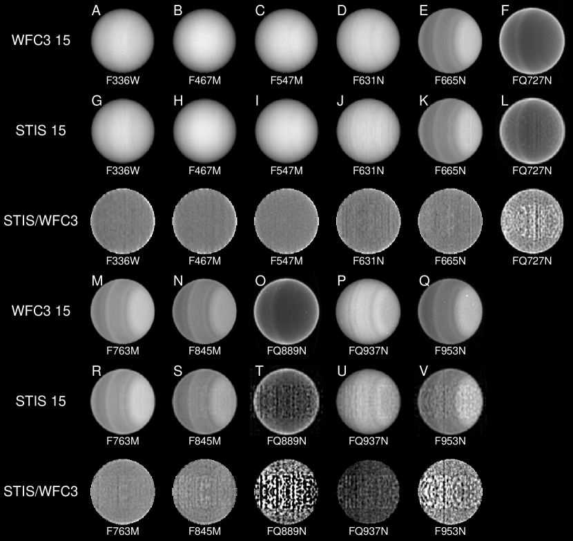
Figure 2.— WFC3 images of Uranus taken on 11 October 2015 (A-F and M-Q) compared to synthetic band-pass filter images (G-L and R-V) created from weighted averages of STIS spectral data cubes using WFC3 throughput and solar spectral weighting. The north pole is at at the right. Portions of the synthetic images east of the central meridian are obtained by reflection of the images west of the central meridian. The ratio images are stretched to make 0.8 black and 1.2 white.

3.3. Supporting near-IR imaging

HST/NICMOS and groundbased Keck and Gemini imaging at near-IR wavelengths help to extend and fill gaps in the temporal record of changes occurring in the atmosphere of Uranus. Fig. 3 shows that the difference between polar and low latitude cloud structures has evolved over time. The relatively rapid decline of the bright “polar cap” in the south and its reformation in the north is faster than seems consistent with the long radiative time constants of the Uranian atmosphere (Conrath et al., 1990). In following sections we will show that the polar brightness in 2015 (and presumably also in 1997) is not due very much to latitudinal variations in aerosol scattering, but is mainly due to a much lower degree of methane absorption at high latitudes. This latitudinal variation of methane absorption appears to be stable over time according to infrared observations (Sromovsky et al., 2014). Thus, at times when the polar region was as dark as low latitudes (compared at the same view angles), it appears not that methane absorption was greater then, but instead that aerosol scattering was reduced, a causal relationship we will here further confirm regarding polar brightness increases between 2012 and 2015.

The aforementioned interpretation of the bright polar region on Uranus can be partly inferred from the characteristics of near-IR images at key wavelengths that have different sensitivities to methane and hydrogen absorption, as illustrated in Fig. 4. Images at hydrogen dominated wavelengths (panels A and E) reveal relatively bright low latitudes, and high latitudes that were either darker, as at equinox (A), or comparably bright, as in 2015 (E). At methane dominated wavelengths, low latitudes are relatively darker, especially in 2015, where the excess methane absorption at low latitudes is obvious from comparing panels E and F.

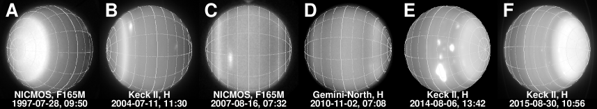
Figure 3.— H-band (1.6-$\mu$m) images of Uranus from 1997 through 2015, from observatories/instruments given in the legends. The bright south polar region seen in 1997 (A), 10 years before equinox, is similar to the bright north polar region seen in 2015 (F), eight years after equinox. Images taken during the 2007 equinox year (C) found that neither polar region was bright. The longitude and planetographic latitude grid lines are at 30^∘ and 15^∘ intervals respectively.

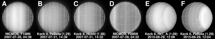
Figure 4.— Near-IR narrow-band images of Uranus obtained near the 2007 equinox (A-D) and in August 2015 (E, F) from observatories/instruments given in the legends. The NICMOS F108N image (A) and the Keck II He1_A image (E) sample wavelengths at which hydrogen absorption dominates. The remaining images sample wavelengths of comparable absorption but due entirely to methane. Note that low latitudes are relatively darker than high latitudes at methane dominated wavelengths (e.g. in B and F), which is not the case for wavelengths dominated by hydrogen absorption (as in A and E). Grid lines are the same as in Fig. 3.

Table 2Near-IR observations from HST, Keck, and Gemini observatories.

Telescope			Obs.		Phase	S.O.
/Instrument	PID	Obs. Date	Time	Filter	Angle	CLat	PI, Notes
HST/NICMOS	7429	1997-07-28	09:50:24	F165M		-40.3	Tomasko, 1
Keck II/NIRC2		2003-10-06	07:14:51	H		-18.1	Hammel, 2
Keck II/NIRC2		2004-07-11	11:30:32	H		-11.1	de Pater, 2
HST/NICMOS	11118	2007-07-28	04:39:xx	F095N	2.0	0.61	Sromosvky, 3
HST/NICMOS	11118	2007-07-28	04:22:30	F095N		0.58	Sromovsky, 3
HST/NICMOS	11118	2007-07-28	04:39:13	F108N		0.58	Sromovsky, 3
Keck II/NIRC2		2007-07-31	14:39:28	PaBeta	1.87	0.51	Sromovsky, 2
Keck II/NIRC2		2007-07-31	14:32:33	Hcont		0.49	Sromovsky, 2
HST/NICMOS	11190	2007-08-16	07:32:32	F165M		-0.0	Trafton, 3
Gemini-N/NIRI	2010B-Q-110	2010-11-02	07:08:57	H_G0203		9.3	Sromovsky, 4
Keck II/NIRC2		2014-08-06	13:42:06	H		28.4	de Pater, 2
Keck II/NIRC2		2015-08-29	12:09:05	He1A		31.96	de Pater, 2
Keck II/NIRC2		2015-08-29	12:04:41	PaBeta		31.96	de Pater, 2
Keck II/NIRC2		2015-08-30	10:56:55	H		31.9	de Pater, 2

NOTES: 1: pscale = 0.0431 as/pixel; 2: pscale = 0.009942 as/pixel ; 3: pscale = 0.0432 as/pixel ; 4: pscale= 0.02138 as/pixel

4. STIS data reduction and calibration.

The STIS pipeline processing used at STScI is just the first step of a rather complex calibration procedure, which is described by KT2009 for the 2002 observations, and by Sromovsky et al. (2014) for the 2012 observations. Essentially the same procedure was followed for the 2015 observations. Additionally, 2002 and 2012 STIS cubes were recalibrated using WFPC2 and WFC3 images newly reduced using the best available detector responsivity functions and filter throughput functions. All three calibrated STIS cubes and related information can be found online in the HST MAST archive as described in the supplemental material section at the end of the paper. In the discussion that follows, we first describe the processing of supporting WFC3 imaging. In the case of 2012 recalibration, WFC3 imaging was also utilized, but for the 2002 recalibration, WFPC2 images were used. We then describe the creation of our calibration correction function, describe our spectral cube construction, and finally our comparison of STIS synthetic images with bandpass filter images.

Each WFC3 image was deconvolved with an appropriate Point-Spread Function (PSF) obtained from the tiny tim code of Krist (1995), optimized to result in data values close to zero in the space view just off the limb of Uranus. To match the spatial resolution of the STIS images, the WFC3 images were then reconvolved with an approximation of the PSF given in the analysis supplemental file of Sromovsky et al. (2014). The images were then converted to I/F using the best available header PHOTFLAM values [given in WFC3 ISR 2016-001] and the Colina et al. (1996) solar flux spectrum, averaged over the WFC3 filter band passes. (PHOTFLAM is a multiplier used to convert instrument counts of electrons/second to flux units of ergs/s/cm²/Å.) To obtain a disk-averaged I/F, the planet’s light was integrated out to 1.15 times the equatorial radius, then averaged over the planet’s cross section in pixels, which was computed using NAIF ephemerides (Acton, 1996) and SPICELIB limb ellipse model (SPICELIB is NAIF toolkit software used in generating navigation and ancillary instrument information files.) The disk-averaged I/F (using the initial calibration) was also computed for each of the STIS monochromatic images, and the filter- and solar flux-weighted I/F was computed for each of the WFC3 filter pass bands that we used.

By comparing the synthetic disk-averaged STIS I/F, using the initial calibration, to the corresponding WFC3 values, we constructed a correction function to improve the radiometric calibration of the STIS cube. Figure 5C shows the ratios of STIS to WFC3 disk-integrated brightness, and the quadratic function that we fit to these ratios as a function of wavelength, for the 2015 data set and recalibrations of the previous two data sets. We heavily weighted the broadband filters, and computed an effective wavelength weighted according to the product of the solar spectrum and the I/F spectrum of Uranus. The RMS deviation of individual filters from the calibration curve given in Fig. 5 is about 1% RMS for 2012 and 2015 correction curves, but about 2 % RMS for the 2002 calibration curve (fit points not shown). For narrow filters such as FQ937N, typical deviations are some three times larger. The difference between the 2002 and the later calibration curves is mostly due to use of different slit locations, which result in different light paths through the monochrometer. The 2012 and 2015 curves use the same slit location and thus should be the same, and indeed they are consistent to about 1%.

If one assumes that the spectrum of Uranus varies only slowly with time, one can add many other filters to plots of Fig. 5 where images are available somewhat close to the time of STIS spectroscopy. The medium and wide filters plot quite consistently near the same curve while many narrow filters show significant offsets, suggesting that an improved calibration weights the narrow filters much less in the fitted curve. This consideration changes the calibration by about 1% and thus does not make a big difference with respect to our previous adopted calibration, but our new calibration is more reliable because it is less dependent on unreliable data from narrow filters.

The final calibrated cubes contain 150 pixels parallel to the spin axis of Uranus and 75 pixels perpendicular to its spin axis, with a spatial sampling interval of of 0.015$\times R_{U}$ km/pixel (384 km/pixel), which is equivalent to 0.028 arc seconds per pixel for 2015 observations. (Here $R_{U}$ is the equatorial radius of Uranus). The center of Uranus is located at coordinates (74, 74), where (0, 0) is the lower left corner pixel. The spatial resolution of the final cube is defined by a point-spread function with a FWHM of 3 pixels. The cube contains an image for each of 1800 wavelengths sampled at a spacing of 0.4 nm, with a uniform spectral resolution of 1 nm. Navigation backplanes are provided, in which the center of each pixel is given a planetographic latitude and longitude, solar and observer zenith angle cosines, and an azimuth angle.

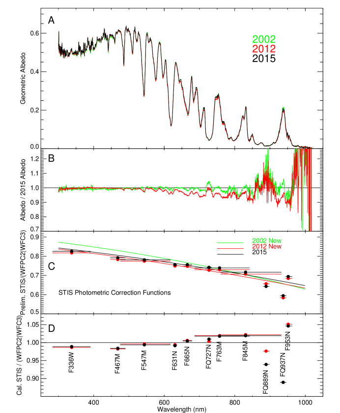
Figure 5.— A: Radiometrically calibrated disk-averaged I/F spectra for three year of STIS observations. STIS observations from 2002 and 2012 have been recalibrated from previous incarnations (Karkoschka and Tomasko, 2009; Sromovsky et al., 2014). B: Ratio of each year’s disk-averaged I/F to 2015. C: STIS photometric calibration functions (raw stis albedo divided by WFC3 albedo). The functions are a fit to ratios constructed using synthetic band-pass filter disk-integrated I/F values (preliminary-calibration) divided by corresponding I/F values obtained from WFC3 measurements (circles and horizontal bars indicate filter effective wavelength and full-width half maximum transmission for 2012 and 2015). D: Ratio of final calibrated STIS synthetic disk-averaged I/F values to WFC3 reflectivities, showing scatter of ratios relative to the fits, for 2012 and 2015.

As a sanity check on the STIS processing we compared WFC3 images to synthetic WFC3 images created from our calibrated STIS data cubes, as shown in Fig. 2. Ratio plots of STIS/WFC3 show the desired flat behavior, except very close to the limbs, where STIS I/F values exceed WFC3 values. The most significant discrepancy is in the overall I/F level computed for the FQ937N filter (note the dark ratio plot in the bottom row), a consequence of our calibration curve being 10% high for that filter.

5. Center-to-limb fitting

The low frequency of prominent discrete cloud features on Uranus and its zonal uniformity make it possible to characterize the smooth center-to-limb profiles of the background cloud structure without much concern about longitudinal variability, even though we observed only half the disk of Uranus. These profiles provide important constraints on the vertical distribution of cloud particles and the vertical variation of methane compared to hydrogen. Because our observations were taken very close to zero phase, these profiles are a function of just one angular parameter, which we take to be $\mu$, the cosine of the zenith angle (the observer and solar zenith angles are essentially equal). They also have a relatively simple structure that we characterized using the same 3-parameter function KT2009 used to analyze the 2002 STIS observations, and which we also used to fit the 2012 observations. For each 1^∘ of latitude from 30^∘ S to 87^∘ N, all image samples within 1^∘ of the selected latitude and with $\mu>$ 0.175 are collected and fit to the empirical function

$$I(\mu)=a+b\mu+c/\mu,$$ (1)

assuming all samples were collected at the desired latitude and using the $\mu$ value for the center of each pixel of the image samples. Fitting this function to center-to-limb (CTL) variations at high latitudinal resolution makes it possible to separate latitudinal variations from those associated with view angle variations.

Before fitting the CTL profile for each wavelength, the spectral data were smoothed to a resolution of 2.88-nm to improve signal to noise ratios without significantly blurring key spectral features. (Our prior analysis was conducted in the wavenumber domain and used smoothing to a resolution of 36 cm^-1.) Sample fits are provided in Fig. 6. Most of the scatter about the fitted profiles is due to noise, which is often amplified by the deconvolution process. Because the range of observed $\mu$ values decreases away from the equator at high southern and northern latitudes, we chose a moderate value of $\mu$ = 0.7 as the maximum view-angle cosine to provide a reasonably large unextrapolated range of 16^∘ S to 77^∘ N. Ranges for other years and for a $\mu$ range of 0.3 to 0.6 are given in Table 3. Unless otherwise noted all our results are derived without extrapolation.

Table 3Latitude ranges for two different view-angle cosine ranges.

Year	0.3 $\leq\mu\leq$ 0.6	0.3 $\leq\mu\leq$ 0.7
2002	74∘S – 33∘N	67∘S – 26∘N
2012	35∘S – 72∘N	28∘S – 65∘N
2015	23∘S – 77∘N	16∘S – 77∘N

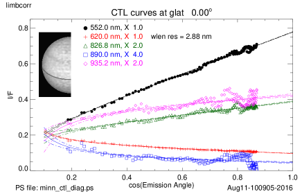
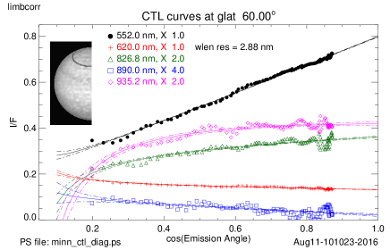
Figure 6.— Sample center-to-limb fits for 0^∘ N (left) and 60^∘N (right), as described in the main text. STIS I/F samples and fit lines with uncertainty bands are shown for five different wavelengths indicated in the legends. The latitude bands sampled for these fits are darkened in the inset images of the half-disk of Uranus.

The CTL fits can also be used to create zonally smoothed images by replacing the observed I/F for each pixel by the fitted value. Results of that procedure are displayed in a later section.

6. Direct comparisons of STIS spectra

A rough assessment of the changes between 2012 and 2015 and the differences between high and low latitudes in these two years can be made with the help of direct comparisons of STIS spectra, as in Fig. 7. Note that at 10^∘ N there is almost no difference between 2012 and 2015 spectra (panels A and B). This is also the case for $\mu$ values of 0.3 and 0.5, which are not shown in the figure. For 2015, (see panel E) the lack of any I/F difference between 10^∘ N and 60^∘ N at 0.83 $\mu$m, which is a wavelength at which hydrogen absorption dominates, suggests that there is not much difference in aerosol scattering between these two latitudes. A similar lack of difference at 0.93 $\mu$m, a wavelength of weak (but dominant) methane absorption, suggests that at very deep levels, there may not be much of a latitudinal difference in methane mixing ratios, or that there is an aerosol layer blocking visibility down to levels that might sense such a difference. Yet the fact that wavelengths of intermediate methane absorption do show a significant increase in I/F with latitude suggests that at upper tropospheric levels the methane mixing ratio does decline with latitude, which is a known result from previous work, and is refined by the analysis presented in following sections. Somewhat different results are seen, for 2012 (in panel G). The 10^∘ N and 60^∘ N I/F values at 0.83 $\mu$m and 0.93 $\mu$m do differ (panels G and H), which we will later show is a result of differences in aerosol scattering. The small size of continuum differences between 2012 and 2015 (panels D and H) is partly a result of the relatively smaller impact of particulates at short wavelengths where Rayleigh scattering is more significant. At absorbing wavelengths for which gas absorption is important, the optical depth and vertical distribution of particulates have a greater fractional effect on I/F and thus small secular changes in these parameters can be more easily noticed.

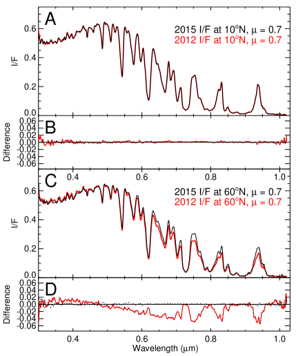
Figure 7.— Comparison of 2012 and 2015 STIS spectra at 10^∘ N (A) and 60^∘ N (C), and comparison of STIS 10^∘ N and 60^∘ N spectra from 2015 (E) and 2012 (G), with difference plots shown in panels B, D, F, and H respectively. The dotted curve in panel H is a copy of the 2015 difference curve from panel F. Latitudes are planetographic. Note the nearly exact equality (in A) of 10^∘ N spectra from 2012 and 2015.

7. Direct comparison of methane and hydrogen absorptions vs. latitude.

If methane and hydrogen absorptions had the same dependence on pressure, then it would be simple to estimate the latitudinal variation in their relative abundances by looking at the relative variation in I/F values with latitude for wavelengths that produce similar absorption at some reference latitude. Although this idea is compromised by different vertical variations in absorption, which means that latitudinal variation in the vertical distribution of aerosols can also play a role, it is nevertheless useful in a semi-quantitative sense. Thus we explore several cases below.

7.1. Image comparisons at key near-IR wavelengths in 2007 and 2015

Our first example compares an HST/NICMOS image made with an F108N filter (centered at 1080 nm), which is dominated by H₂ CIA, to a KeckII/NIRC2 image made with a PaBeta filter (centered at 1290 nm), which is dominated by methane absorption. The images are shown in panels A and B in Fig. 4 and latitude scans at fixed view angles are shown in Fig. 8. The NICMOS observation was taken on 28 July 2007 at 4:39 UT and the Keck observation on 31 July 2007 at 14:39 UT (see Table 2 for more information). That these two observations sense roughly the same level in the atmosphere is demonstrated by the penetration depth plot in Fig. 1, which also displays the filter transmission functions. The absolute (unscaled) I/F profiles for these two images near the 2007 Uranus equinox are displayed for $\mu$ = 0.6 and $\mu$ = 0.8 by thinner lines in Fig. 8. At high latitudes in both hemispheres, profiles at the two wavelengths agree closely, and both increase towards the equator. But as low latitudes are approached the two profiles diverge dramatically, with the I/F for the hydrogen-dominated wavelength ending up 50% greater than for the methane-dominated wavelength, indicating much greater methane absorption at low latitudes than at high latitudes. As noted by Sromovsky et al. (2014) this suggests that upper tropospheric methane depletion (relative to low latitudes) was present at both northern and southern high latitudes in 2007, at least roughly similar to the pattern that was inferred by Tice et al. (2013) from analysis of 2009 IRTF SpeX observations. Latitudinal variations in aerosol scattering could distort these results somewhat, but because they affect both wavelengths to similar degrees, most of the effect is likely due to methane variations.

Figure 8.— Latitudinal profiles at fixed zenith angle cosines of 0.6 (A) and 0.8 (B) for F108N (HST/NICMOS) and PaBeta (Keck/NIRC2) filters (light solid and dashed lines respectively) taken near the Uranus equinox in 2007, and Keck/NIRC2 filter He1_A and PaBeta filters (thick solid and dashed lines respectively) in 2015. In 2007 the southern hemisphere was still generally brighter than the northern hemisphere and the 38^∘ S - 58^∘ S southern bright band was still better defined and considerably brighter than the corresponding northern bright band. The relatively low equatorial I/F values for the methane-dominated PaBeta filter (1290 nm) implies greater CH₄/H₂ absorption at low latitudes. We scaled the Keck 2015 observations to approximately match the 2007 observations at 10^∘N, where we found almost no change between 2012 and 2015 at CCD wavelengths (Fig. 7A). Note that between 2007 and 2015, the north polar region has brightened by comparable amounts at both hydrogen-dominated and methane-dominated wavelengths, indicating that it the brightening is due to increased aerosol scattering, not a temporal change in the methane mixing ratio at high latitudes. More information about the observations is given in Table 2.

A second example is shown by the thicker lines in Fig. 8, which display latitudinal scans of 2015 images shown in panels E and F of Fig. 4. These were made by the KeckII/NIRC2 camera with He_1A and PaBeta filters on 29 August 2015 (see Table 2). The He_1A filter is similar to the NICMOS F108N filter, as shown in Fig. 1. The 2015 observations present a picture that is somewhat different from the 2007 observations, with high northern latitudes much brighter (at the same view angles) than in 2007. This change appears to be entirely due to increased aerosol scattering. This conclusion is supported by the characteristics of images obtained with H₂-dominated filters (NICMOS F108N filter and Keck He1_A filter). In 2015 the I/F in the He1_A filter is relatively independent of latitude as shown by the image in panel E of Fig. 4, indicating that aerosol scattering must have a relatively weak latitudinal dependence. Note that latitude scans at fixed view angles for these filters (shown in Fig. 8) exhibit a low-latitude divergence of the hydrogen-dominated and methane-dominated wavelengths which has about the same magnitude in 2015 as seen for the 2007 observations, indicating a similar increase of methane absorption at low latitudes.

7.2. Direct comparison of key STIS wavelength scans

A comparison of the STIS latitude scans at methane dominated wavelengths with scans at H₂ CIA dominated wavelengths is also informative. By selecting wavelengths that at one latitude provide similar I/F values but very different contributions by H₂ CIA and methane, one can then make comparisons at other latitudes to see how I/F values at the two wavelengths vary with latitude. If aerosols did not vary at all with latitude, then any observed I/F variation would be a clear indicator of variation in the ratio of CH₄ to H₂. Fig. 9 displays a detailed view of I/F in the spectral region where hydrogen CIA exceeds methane absorption (see Fig. 1 for penetration depths). Near 827 nm (A) and 930 nm (C) the I/F values are similar but the former is dominated by hydrogen absorption (dot-dash curve) and the latter by methane absorption (dashed curve). Near 835 nm (B) there is a relative minimum in hydrogen absorption, while methane absorption is still strong. For the latitude and view angle of this figure (50^∘ N and $\mu$ = 0.6), I/F values are nearly the same at all three wavelengths, suggesting that they all produce roughly the same attenuation of the vertically distributed aerosol scattering.

Figure 9.— I/F and absorption spectra comparing the equilibrium H₂ CIA coefficient spectrum (divided by 1.2$\times 10^{-7}$, shown as dot-dash curve) and methane absorption coefficient spectrum (dashed). Note that the I/F spectrum has nearly equal I/F values at 826.8 nm (A), 834.6 nm (B), and 930 nm (C), but H₂ absorption is much greater at A than at B, while the opposite is true of methane absorption, and at C only methane absorption is present. In a reflecting layer model, changes in cloud reflectivity should affect wavelengths A-C by the same factor, but changes in methane mixing ratio would affect C most and A least. From Sromovsky et al. (2014).

Figure 10 displays the latitudinal scans for the three wavelengths highlighted in Fig. 9 for the STIS observations in 2002 (shown by thin lines), 2012 (thick gray lines), and 2015 (thick black lines). This is for a view angle cosine of $\mu=0.6$, chosen as a compromise between amplitude of variation and coverage in latitude. The 2012 I/F for the hydrogen-dominated wavelength increases towards low latitudes, while the I/F for the methane-dominated wavelength decreases substantially, indicating an increase in the amount of methane relative to hydrogen at low latitudes. Similar effects are seen in 2002 (providing the best view of southern latitudes) and 2015 (providing the best view of the northern latitudes). The hydrogen-dominated wavelengths have relatively flat latitudinal profiles of I/F in the southern hemisphere in 2002 and in the northern hemisphere in 2015, while the methane-dominated wavelengths show strong decreases towards the equator, beginning at about 45^∘ S and 50^∘ N. For $\mu$=0.8 (not shown), which probes more deeply, the latitudinal variation for the methane dominated wavelengths is somewhat greater (a 30% decrease in I/F at low latitudes vs. a 20% decrease for $\mu$ = 0.6).

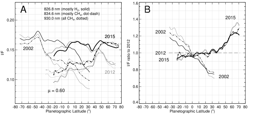
Figure 10.— I/F vs. latitude at $\mu=0.6$ (A) and ratio of I/F scans to the 2012 scans (B) for three wavelengths with different amounts of methane and hydrogen absorption. Thin curves are from 2002, thick gray curves from 2012, and thick black curves from 2015. These are plots of center-to-limb fitted values instead of raw image data. In all cases the methane-dominated wavelengths have much reduced I/F at low latitudes, compared to hydrogen-dominated wavelengths, indicating higher CH₄ /H₂ ratios at low latitudes. Also note the increased north polar brightness at all displayed wavelengths between 2012 and 2015, indicating that the temporal change is due to increased aerosol scattering.

The spectral comparisons in Fig. 10 also reveal substantial secular changes between 2002 and 2012 and between 2012 and 2015. At wavelengths for which methane and/or hydrogen absorption are important, the northern low-latitudes have brightened substantially, while the southern low latitudes have darkened. The bright band between 38^∘ and 58^∘ N continued to brighten. Its brightening and the darkening of the corresponding southern band was already apparent from a comparison of 2004 and 2007 imaging (Sromovsky et al., 2009). The most dramatic change between 2012 and 2015 is the increased brightness of the polar region. The nearly identical brightening at all wavelengths, shown by the ratio plot in panel B of Fig. 10, argues that the brightening is due to aerosol scattering rather than a decrease in the amount of methane. We will confirm this with radiation transfer modeling in Section 9.

A color composite of the highlighted wavelengths (using R = 930 nm, G = 834.6 nm, and B = 826.8 nm) is shown in Fig. 11, where the three components are balanced to produce comparable dynamic ranges for each wavelength. This results in nearly blue low latitudes where absorption at the two methane dominated wavelengths is relatively high and green/orange polar regions as a result of the decreased absorption by methane there. The spatial structure in high-resolution near-IR H-band Keck II images is also shown in each panel, revealing that small discrete cloud features remain visible in the north polar regions even in the 2015 images, taken after the polar region brightened significantly between 2012 and 2015. Also noteworthy, is the lack of such features in the south polar region (panel A). This asymmetry is somewhat surprising. As noted by Sromovsky et al. (2014), because both polar regions are depleted in methane, the suggested downwelling motions that could produce such depletion would be expected to inhibit convection in both polar regions.

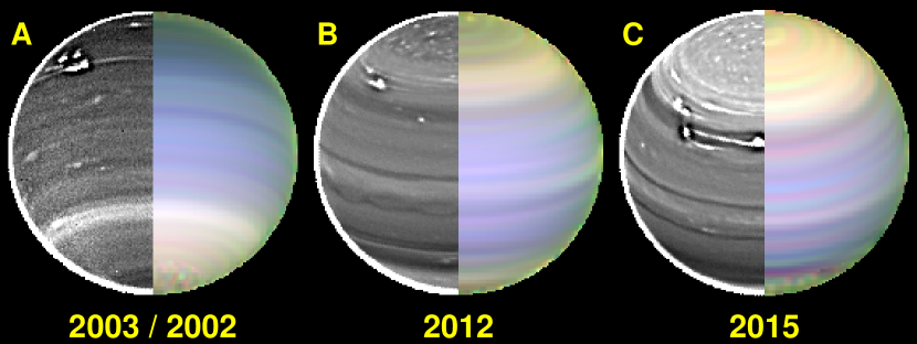
Figure 11.— Color composites of fitted center-to-limb smoothed images for 2002 (A, right), 2012 (B, right), and 2015 (C, right), using color assignments R=930 nm (all methane) G=834.6 nm (methane and hydrogen), and B=826.8 nm (mostly hydrogen). The blue tint at low latitudes in all years is due to locally increased methane absorption. We also show near-IR NIRC2 H-band images for 2003 (A, left), 2012 (B, left), and 2015 (C, left). The NIRC2 images are rotation removed averages following Fry et al. (2012) and processed to enhance the contrast of small spatial scales, by adding k times the difference between the original image and a 0.13-arcsecond smoothed version, where k was taken to be 30 for 2003 and 2012 images, but only 22.5 for the 2015 image because of better seeing conditions during its acquisition.

8. Radiative transfer modeling of methane and aerosol distributions

8.1. Radiation transfer calculations

In contrast to our prior analysis (Sromovsky et al., 2014), which was carried out in the wavenumber domain to accommodate our Raman scattering code, here we worked in the wavelength domain, which is better suited to the uniform wavelength resolution of our calibrated STIS data cubes. We also used an approximation for the effects of Raman scattering rather than carrying out the full Raman scattering calculations. We again used the accurate polarization correction described by Sromovsky (2005b) instead of carrying out the time consuming rigorous polarization calculations. To assess the adequacy of our approximations, we did sample calculations that included Raman scattering and polarization effects on outgoing intensity using the radiation transfer code described by Sromovsky (2005a). Examples in Fig. 12 show that at most wavelengths the errors from these approximations do not exceed a few percent.

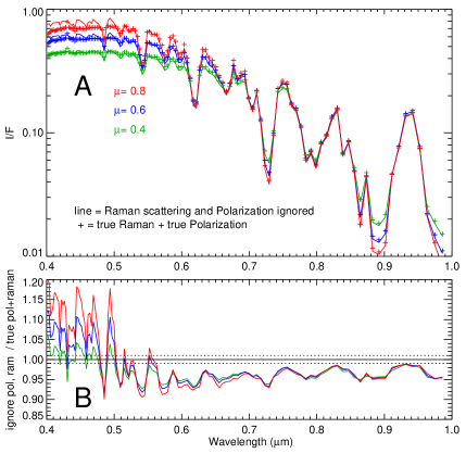
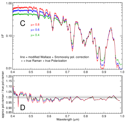
Figure 12.— Trial calculations showing errors produced by ignoring Raman scattering and polarization (A and B) and greatly reduced errors achieved by employing the modified Wallace approximation of Raman scattering (Sromovsky, 2005a) and the approximation of polarization effects following Sromovsky (2005b).

We improved our characterization of methane absorption at CCD wavelengths by using correlated-k model fits by Irwin et al. (2010), which are available at http://users.ox.ac.uk/$\sim$atmp0035/ktables/ in files ch4_karkoschka_IR.par.gz and ch4_karkoschka_vis.par.gz. These fits are based on band model results of Karkoschka and Tomasko (2010). To model collision-induced opacity of H₂-H₂ and He-H₂ interactions, we interpolated tables of absorption coefficients as a function of pressure and temperature that were computed with a program provided by Alexandra Borysow (Borysow et al., 2000), and available at the Atmospheres Node of NASA’S Planetary Data System. We assumed equilibrium hydrogen, following KT2009 and Sromovsky et al. (2011).

After trial calculations to determine the effect of different quadrature schemes on the computed spectra, we selected 12 zenith angle quadrature points per hemisphere and 12 azimuth angles. Test calculations with 10 and 14 quadrature points in each variable changed fit parameters by only about 1%, which is much less than their uncertainties.

8.2. Thermal profiles for Uranus

Assuming the helium volume mixing ratio (VMR) of 0.152 inferred by Conrath et al. (1987), Lindal et al. (1987) used radio occultation measurements of refractivity versus altitude to infer a family of thermal and methane profiles, with each profile distinguished by the assumed methane relative humidity above the cloud level, and the resultant deep volume mixing ratio (VMR) of methane below the cloud level. The cloud was positioned at the point where the refractivity profile had a sharp change in slope. None of these profiles achieved methane saturation inside the cloud layer, even the profile with the highest physically realistic humidity level (limited by the requirement that lapse rates could not be superadiabatic). This high-humidity profile also had the highest deep temperatures and the largest deep methane VMR of 4%. By allowing the He/H₂ ratio to take on values near the low end of the uncertainty range given by Conrath et al. (1987), Sromovsky et al. (2011) were able to find solutions that achieved methane saturation inside the cloud layer, as well as deep methane mixing ratios somewhat greater than 4%.

The above results are based on the Voyager ingress profile, which sampled latitudes from 2^∘S to 6^∘S. As to whether this local sample can be taken to roughly represent a global mean profile, some guidance is provided by the results that Hanel et al. (1986) derived from the Voyager 2 Infrared Interferometer Spectrometer (IRIS) observations. Inversion of spectral samples near both poles and near the equator yielded temperature profiles that differed by less than 1 K from about 150 mbar to 600 mbar, and the equator and south pole profiles remained within 2 K from 60 mbar to 150 mbar, with the north polar profile deviating up to 4 K above the tropopause. More significant variations can be seen at middle latitudes, however, especially in the 60 – 200 mbar range where average temperatures are 3.5 K higher than the latitudinal average near the equator and 4.5 K lower near 30^∘S (Conrath et al., 1991). In the 200 – 1000 mbar range latitudinal excursions are within 1–1.5 K. Thus it appears that in the most important region of the atmosphere for our applications, the thermal structure was not strongly variable with latitude, at least in 1986. Models of seasonal temperature variations on Uranus by Friedson and Ingersoll (1987) suggest that the effective temperature variation at low latitudes will be extremely small, only 0.2 K peak-to-peak at the equator, increasing to a still relatively small 2.5 K at the poles. Thus, it is plausible to analyze observations during the 2012 – 2015 period with thermal profiles obtained as far back as 1986, even though they are local, but probably more appropriate to use thermal structures derived from observations in 2007, averaging over a wide range of latitudes, such as those inferred by Orton et al. (2014a) from nearly disk-integrated spectral observations.

Sample thermal and methane profiles are displayed in Fig. 13. The profile of Orton et al. (2014a), hereafter referred to as O14, is based on nearly disk-integrated spectral observations obtained with the Spitzer Space Telescope near the Uranus equinox in 2007. Among the occultation profile sets, it is only those with high methane VMR values that provide decent agreement with the O14 deep temperature structure, but none of the occultation profiles are compatible with the O14 profile in the 0.30 – 1.0 bar range. One might argue that if radio occultation results agree with O14 at 100 mb and at pressures beyond 1 bar, then the disagreement in temperatures at intermediate pressure levels is more likely due to an error in the Orton et al. profile because that profile is inferred from different spectrometers in different spectral regions that sample different altitudes, which might suffer from differences in calibrations, while the radio occultation uses the same measurement (the frequency of a radio signal) throughout the pressure range. It seems more likely that the errors in the radio profile would be in the altitude scale or in offsets due to uncertain He/H₂ ratios, rather than varying in the way the differences between the radio and Orton et al. profile do. A similar argument might be made in favor of the Conrath et al. (1987) profile over the O14 profile because the former is based on interferometric measurements using the same instrument over the entire spectral range. And the former profile is in good agreement with the occultation-based profiles in the 300–600 mbar range, where the latter is not. On the other hand, the Orton et al. profile allows higher CH₄ mixing ratios without saturation in the 0.3 – 1 bar region (Fig. 13) and are thus more compatible with the recent Lellouch et al. (2015) CH₄ VMR profile derived from Herschel far-IR and sub mm observations.

The methane VMR in the stratosphere was estimated to be no greater than $10^{-5}$ by Orton et al. (1987). A best fit estimate for the tropopause value of the methane VMR, based on more recent Spitzer observations, is $(1.6^{+0.2}_{-0.1})\times 10^{-5}$ according to Fig. 4 of Orton et al. (2014b), which is the value we assumed here in deriving the new F0 profile. However, the even more recent Lellouch et al. (2015) result is three times larger. In terms of relative humidity (ratio of vapor pressure to saturation vapor pressure) these stratospheric mixing ratios correspond to humidities of 25% and 75% at the Orton et al. tropopause temperature of 52.4 K. The F profile of Lindal et al. (1987) was derived assuming a constant methane relative humidity of 53% above the cloud tops and a constant stratospheric mixing ratio equal to the tropopause value. In deriving the F0 profile we used linear-in-altitude interpolation of the methane humidity values between the cloud top and tropopause. The F1 profile of Sromovsky et al. (2011) followed the same procedure except that the value of the tropopause mixing ratio was taken to be the earlier upper bound of $10^{-5}$ and the He VMR was taken to be 0.1155 instead of 0.152. The lower He VMR was chosen to produce a saturated methane mixing ratio inside the cloud layer.

Our analysis for this paper is primarily based on the O14 thermal profile, although we did consider the effects of using these alternative profiles. From trial retrievals we found no significant difference in the absolute mixing ratios inferred for different thermal profiles. The main differences occurred when these mixing ratios were converted to relative humidities. We often found supersaturation above the condensation level for the cooler occultation profiles, whereas the same mixing ratios did not lead to supersaturation for the warmer O14 profile, or for the F0 profile. The F0 profile would also have been a decent baseline choice, as long as we did not also use the F0 methane profile, and instead let the STIS spectra constrain the methane mixing ratios without regard to occultation consistency.

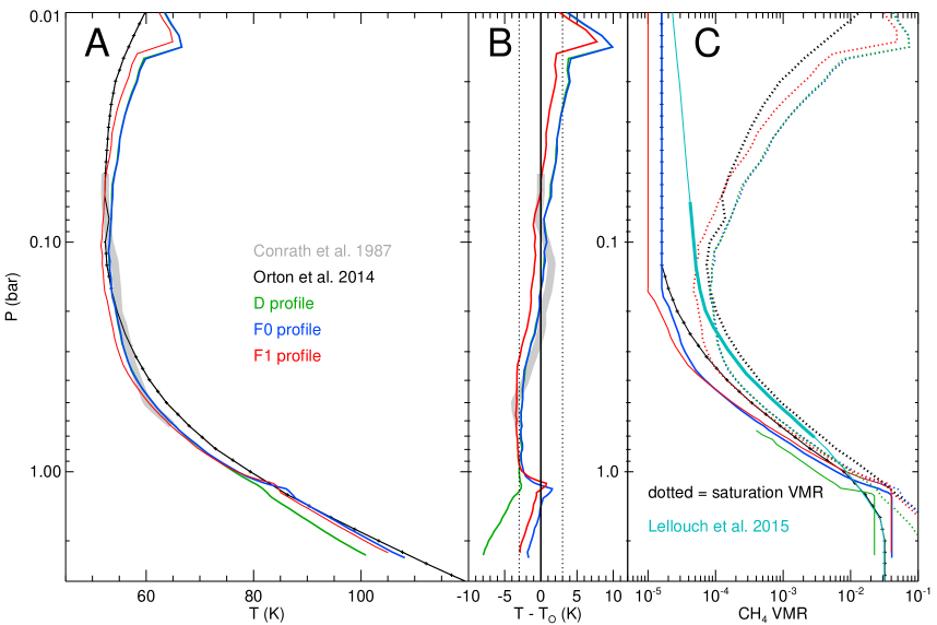
Figure 13.— A: Alternate Uranus T(P) profiles. F0 and D profiles were derived from radio occultation measurements (Lindal et al., 1987) assuming a helium VMR of 0.152. The F1 profile was also derived from radio occultation measurements, but using a lower helium VMR 0.1155, following Sromovsky et al. (2011). The Voyager IRIS profile of Conrath et al. (1987) (thick gray curve) is in best agreement with the F0, D, and F1 profiles. The Orton et al. (2014a) profile (solid black curve), is based on Spitzer Space Telescope spectral observations. B: Temperatures relative to the Orton et al. (2014a) profile, which strongly disagrees with the radio occultation profiles in 500 mbar – 1 bar region, where it is 3 K warmer. C: Methane VMR profiles corresponding to temperature profiles shown in A, using the same line styles, with an additional estimated profile by Lellouch et al. (2015), based on Herschel far-IR and sub-mm observations.

8.3. Vertical Profiles of Methane

In our prior analysis the vertical profile of methane was generally coupled to the vertical temperature profile so that the vertical variation of atmospheric refractivity was consistent with occultation measurement of refractivity. In our current analysis we uncoupled temperature and methane profiles because of questions raised about the reliability of the occultation results, especially by the new temperature structure results of Orton et al. (2014a), and by the new methane measurements of Lellouch et al. (2015), which imply supersaturation for the cooler temperature profiles obtained from occultation analysis. Another difference in our current analysis is that we included the parameters describing the methane vertical distribution as adjustable parameters in the fitting process. We first carry out fits of spectra at different latitudes assuming a vertically invariant (but adjustable) methane VMR ($\alpha_{0}$) below the condensation level. Slightly above the condensation level we fit a relative humidity $rh_{c}$, and assume a minimum relative humidity of $rh_{m}$ at the tropopause between 20% and 60%, which yields mixing ratios within a factor of two of Orton et al. (2014a)). The high end of this range is in better agreement with Lellouch et al. (2015). The STIS spectra themselves are not very sensitive to the exact value at the tropopause, as evident from Fig. 1. Between the tropopause and the condensation level we interpolate relative humidity between $rh_{c}$ and $rh_{m}$ using the function

$$rh(P)=rh_{m}+(rh_{c}-rh_{m})\times$$ (2)

$$\big{[}1-\log(P_{c}/P)/\log(P_{c}/P_{m})\big{]},$$

where $P_{c}$ is the pressure at which CH₄ condensation would occur for the given thermal profile and a given uniform deep methane VMR, and $P_{m}$ is the pressure at which the relative humidity attains its minimum value near the tropopause. Given a deep methane VMR ($\alpha_{0}$) and a temperature profile from which a condensation pressure can be defined, Eq. 8.3 then defines a methane VMR as a function of pressure for $P<P_{c}$, denoted by $\alpha(P)$. That profile is generated prior to application of the Sromovsky et al. (2011) “descended profile” function in which the initial mixing ratio profile $\alpha(P)$ is dropped down to increased pressure levels $P^{\prime}(\alpha)$ using the equation

$$P^{\prime}=P\times[1+(\alpha(P)/\alpha_{0})^{vx}(P_{d}/P_{c}-1)]$$ (3)

$$\mathrm{for}\quad P_{tr}<P<P_{d},$$

where $P_{d}$ is the pressure depth at which the revised mixing ratio $\alpha^{\prime}(P)=\alpha(P^{\prime})$ equals the uniform deep mixing ratio $\alpha_{0}$, $P_{c}$ is the methane condensation pressure before methane depletion, $P_{tr}$ is the tropopause pressure (100 mb), and the exponent $vx$ controls the shape of the profile between 100 mb and $P_{d}$. Sample plots of descended profiles are displayed in Fig. 14. The profiles with $vx=1$ are similar in form to those adopted by Karkoschka and Tomasko (2011). Our prior analysis obtained the best fits with $vx$=3, while our current analysis obtains a latitude dependent value ranging from $\geq$ 9 at low latitudes to 2.4$\pm$0.7 at 70^∘ N.

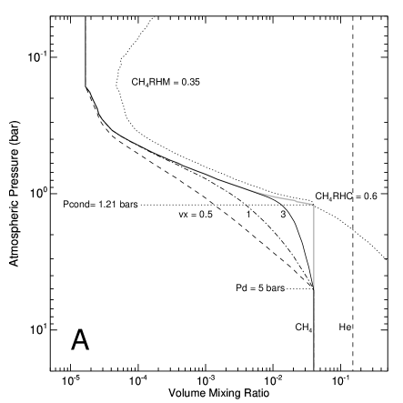
Figure 14.— A: Sample “descended gas” methane profiles with $pd$ = 5 bars and $vx=$ 0.5 (dashed), 1 (dot-dash), and 3 (solid). The starting profile before descent is shown in solid gray and is based on the F1 T(P) profile with methane constrained by its deep mixing ratio and the humidities above the condensation level (CH₄RHC) and at the tropopause (CH₄RHM), with linear in log P interpolation between these levels. B: Sample step-function vertical methane profile using the T(P) profile of Orton et al. (2014a) to define the saturation vapor pressure profile (dotted curve). This particular example fits the 2015 spectra at 40^∘N. See text for further explanation.

Fig. 14B displays an alternative step-function depletion model in which the methane mixing ratio decreases from the deep value to a lower vertically uniform value beginning at pressure $P_{d}$ and continuing upward until the condensation level is reached for that mixing ratio. This is parameterized by four variables: the deep mixing ratio $\alpha_{0}$, the pressure break-point $P_{d}$ , the upper mixing ratio $\alpha_{1}$, and the relative humidity immediately above the condensation level $rh_{c}$. The parameters of all three of these vertical profile models are summarized in Table 4.

Table 4Methane vertical profile model parameters.

Model Type	Parameter (description)	Value
	$\alpha_{0}$ (deep mixing ratio)	adjustable
	$P_{c}$ (condensation pressure)	derived from $\alpha_{0}$, $P(T)$ profile
uniform deep	$P_{t}$ (tropopause pressure)	derived from $P(T)$ profile
	$rh_{c}$ (relative humidity at $0.95\times P_{c}$)	adjustable
	$rh_{m}$ (relative humidity at $P_{t}$)	adjustable, or from Orton et al. (2014a)
	$\alpha_{0}$ (mixing ratio for $P>P_{d}$)	adjustable
	$\alpha_{1}$ (mixing ratio for $P_{c}<P<P_{d}$)	adjustable
	$P_{d}$ (transition pressure)	adjustable
2-step uniform	$P_{c}$ (condensation pressure)	derived from $\alpha_{1}$, $P(T)$ profile
	$rh_{c}$ (relative humidity at $0.95\times P_{c}$)	adjustable
	$rh_{m}$ (relative humidity at $P_{t}$)	fixed at various values
	$\alpha_{0}$ (mixing ratio for $P>P_{d}$)	adjustable
	$P_{d}$ (transition pressure)	adjustable
descended	$vx$ (exponent of shape function)	adjustable
	$\alpha^{\prime}(P)$ (descended VMR profile)	derived by inverting Eq. 8.3
	$rh_{c}$ (relative humidity at $0.95\times P_{c}$)	adjustable
	$rh_{m}$ (relative humidity at $P_{t}$)	fixed at various values

NOTE: we assumed the same mixing ratio for $P<P_{t}$ as for $P=P_{t}$. For the 1 and 2-step uniform models $rh(P)$ for $P_{t}<P<0.95\times P_{c}$ is obtained from Eq. 8.3.

8.4. Cloud models

8.4.1 Prior cloud models

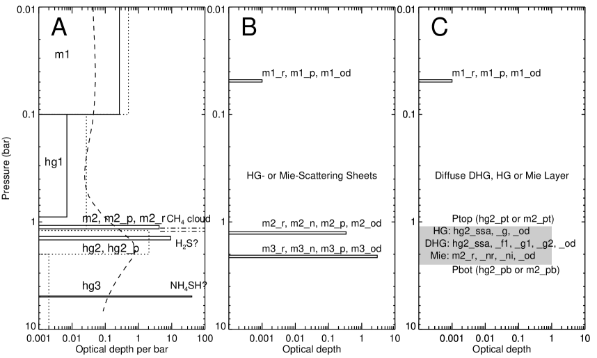
Figure 15.— A: Comparison of the KT2009 model (dotted) with the similar but more complex 5-layer model used by Sromovsky et al. (2014), which replaced two diffuse layers with 3 compact layers. B: A preliminary simplified model with three compact layers, mostly defined by the two lower layers. This model was constructed with the possibility in mind that $m2$ might be formed from methane and $m3$ from H₂S. C: Our baseline simplest model in which the tropospheric cloud is uniformly mixed between top and bottom pressures and has the same particle properties throughout layer 2.

Our prior analysis used an overly complex five-layer model that was based on the KT2009 four-layer model, with the main difference being replacement of their main Henyey-Greenstein (HG) layer with two layers, the higher of which was a Mie-scattering layer that was a putative methane condensation cloud, as illustrated in Fig. 15A. In this model the scattering properties of the three remaining Henyey-Greenstein layers were taken from KT2009, with no adjustment to improve fit quality. This model was partly based on parameters tuned to fit the 2002 STIS observations, taken 13 years before our most recent ones, and thus it was appropriate to reconsider the aerosol structure. In addition, the five-layer model actually has too many parameters to meaningfully constrain independently with STIS observations. Our starting point consisted of three Mie-scattering sheet clouds, as illustrated in Fig. 15B. But we obtained fits of comparable quality using for the tropospheric aerosols a simpler single cloud of uniform scattering properties and uniformly mixed with the gas between top and bottom boundaries, as in in Fig. 15C. As a result, that simpler model became our baseline model. Tice et al. (2013), Irwin et al. (2015), and de Kleer et al. (2015) were successful in using a similar model structure to fit near-IR spectra.

8.4.2 Simplified Mie-scattering aerosol models

We have two options for our 2-cloud baseline model displayed in Fig. 15C. Both options use a sheet cloud of spherical Mie-scattering particles to approximate the stratospheric haze contribution. The parameters defining a sheet cloud of spherical particles are the size distribution of particles, their refractive index, effective pressure, and optical depth. We chose the Hansen (1971) gamma distribution, characterized by an effective radius and effective dimensionless variance. As spectra are not very sensitive to the variance, we chose an arbitrary value of 0.1. Based on preliminary fits we chose a particle size of 0.06 $\mu$m. Other researchers have selected a slightly larger size of 0.1 $\mu$m. We also found generally low sensitivity to the effective pressure as long as it was sufficiently low. We thus chose a somewhat arbitrary value of 50 mbar, putting the haze above the tropopause. We made an arbitrary choice of 1.4 for the layer’s refractive index. At wavelengths shorter than our lower limit, the haze undoubtedly provides some absorption, as noted by KT2009, but we did not need to include stratospheric haze absorption to model its effects in our spectral range. Usually the only adjustable parameter for this layer we took to be the optical depth. Test calculations showed that an extended haze spanning pressures from 1 mbar to 200 mbar worked almost as well as our sheet cloud model. It did produce a slightly larger $\chi^{2}$ but using a diffuse stratospheric haze model had little effect on derived parameter values. The optical depth of the haze only increased by 2%, and the fractional changes in all the other fitted parameters were less than 0.4%, putting these changes well below their estimated uncertainties. In any case, our aim with the haze model was to account for its spectral effects, not to accurately describe the physical characteristics of the haze itself.

For a tropospheric sheet cloud of conservative particles the fitted parameters would be particle size, real refractive index, effective pressure, and optical depth (4 parameters). For a pair of tropospheric sheet clouds, as in Fig. 15B, there would be 8 parameters to constrain. Assuming both layers had the same scattering properties, that would drop the number of fitted parameters to 6. Replacing the pair of sheet clouds with a single diffuse layer with uniform scattering properties, as in Fig. 15C, reduces the number of optical depths to one, but keeps the number of pressure parameters to two, this time used for top and bottom boundaries, yielding a new total of 5 parameters for the tropospheric aerosols. Instead of fitting top and bottom pressures to control the vertical distribution, Tice et al. (2013) chose to fit the base pressure and the particle to gas scale height ratio. Which approach is more realistic remains to be determined. At this point we have a nominal total of 6 adjustable parameters to describe our aerosol particles, one for the stratospheric sheet, and five for the vertically extended tropospheric layer. These are named $m1\_r$, $m2\_r$, $m2\_pb$, $m2\_pt$, $m2\_od$, and $m2\_nr$, where the characters preceding the number indicate the type of particle ($m$ denotes Mie scattering spherical particle), the number is the layer number, and the type of parameter is indicated after the underscore ($r$ for radius, $pb$ for bottom pressure, $pt$ for top pressure, $od$ for optical depth, and $nr$ for real refractive index).

For these spherical (Mie-scattering) particles, wavelength dependent properties are controlled by particle size and refractive index. Even if both of these are wavelength-independent, scattering cross section (or optical depth) and phase function do have a wavelength dependence because of the physical interaction of light with spherical particles. Where our chosen parameters fail to provide sufficient wavelength dependence, we will also add another parameter, namely the imaginary refractive index $m2\_ni$, which will in general be wavelength dependent, and have its main influence over the single-scattering albedo $\varpi$. We also have between two and four parameters chosen to constrain the vertical methane profile, yielding generally between eight and ten total parameters to constrain by the non-linear regression routine.

8.4.3 Non-spherical aerosol models.

Because the particles in the atmosphere of Uranus are thought to be mostly solid particles, they are unlikely to be perfect spheres, and thus we also considered a more generalized description of their scattering properties. To investigate non-spherical scattering, we employed the commonly used double Henyey-Greenstein phase function, in which three generally wavelength-dependent parameters need to be defined: the scattering asymmetry parameter ($g_{1}>0$) of a mainly forward scattering term, the asymmetry parameter ($g_{2}<0$) of the mainly backscattering term, and their respective fractional weights ($f_{1}$ and $1-f_{1}$ respectively). An additional fourth parameter is the single-scattering albedo ($\varpi$), which might also be wavelength dependent. The double Henyey-Greenstein (DHG) phase function is given by

$$P(\theta)=\!f_{1}\!\times\!(1-g_{1}^{2})/(1+g_{1}^{2}-2g_{1}\cos(\theta))^{3/2}\quad$$ (4)

$$+(1-f_{1})\times(1-g_{2}^{2})/(1+g_{2}^{2}-2g_{2}\cos(\theta))^{3/2},$$

where $\theta$ is the scattering angle. KT2009 modeled their results assuming $g_{1}=0.7$ and $g_{2}=-0.3$ and used a wavelength-dependent $f_{1}$ to adjust the phase function of their tropospheric cloud layers so that they would appear relatively bright enough at short wavelengths. For haze layers composed of fractal aggregate particles, as inferred to exist in Titan’s atmosphere, one would expect both phase function and optical depth to be wavelength dependent, and modeling the fractal aggregate phase function variation with double Henyey-Greenstein functions would require wavelength dependence in $g_{1}$ and $g_{2}$ as well as $f_{1}$, judging from the aggregate models of Rannou et al. (1999). An alternate approach to matching observed spectra with spherical particles is to make the particles absorbing at longer wavelengths and conservative at shorter wavelengths.

The simplest DHG particle is just an HG particle characterized by an asymmetry parameter g, and a single scattering albedo $\varpi$, and for a limited spectral range, a wavelength dependence parameter, which can be taken as a linear slope in optical depth, which amounts to three parameters ($g$, $\varpi$, d$\tau$/d$\lambda$). This is the same number needed to characterize scattering by a Mie particle ($r$, $nr$, $ni$). However, if we use a full DHG formulation, then there are five particle parameters to constrain ($f_{1}$, $g_{1}$, $g_{2}$, $\varpi$, and d$\tau$/d$\lambda$).

An alternative way to produce the wavelength dependence of a spherical particle without its potentially complex phase function, containing features like glories and rainbows, which would not be seen in randomly oriented solid particles, is to follow the procedure of Irwin et al. (2015). They computed scattering properties of spherical particles to determine the wavelength dependence of the scattering cross section, but fit the phase function to a double HG function to smooth out the spherical particle features. The refractive index they assumed was the typical value of 1.40 at short wavelengths, but was modified by the Kramers-Kronig relation to be consistent with the fitted variation of the imaginary index. Whether there are any cases of randomly oriented solid particles actually displaying these modified Mie scattering characteristics remains to be determined.

8.4.4 Fractal aggregate particles

For those layers that are produced by photochemistry, it is also plausible that the hazes might consist of fractal aggregates, which have phase functions that are strongly peaked in the forward direction, but are shaped at other angles by the scattering properties of the monomers from which the aggregates are assembled. It is a convenience to assume identical monomers, and to parameterize the aggregate scattering in terms of the number of monomers, the fractal dimension of the aggregate, and the potentially wavelength dependent real and imaginary refractive index of the monomers (Rannou et al., 1999). If the refractive index were wavelength independent, this would require fitting of potentially five parameters (rm, Nm, dim, nr, ni), the same number as for the most general DHG particle. Assuming ni = 0, rm = fixed size, this would require fitting just three parameters (Nm, dim, nr), a tractable task, but one which we have not so far implemented in our fitting code.

To better understand the wavelength dependent properties of aggregates we made some sample calculations. We first considered an aggregate of 100 monomers 0.05 $\mu$m in radius with a real refractive index of 1.4, and a fractal dimension of 2.01. These particles have the mass of a particle of 0.23 $\mu$m in radius. This provides a physical connection between monomer parameters and the wavelength dependent aggregate phase function and scattering and absorption cross sections. We found that it is possible to at least roughly characterize the fractal aggregate phase functions with double Henyey-Greenstein functions, although this provides no physical connection to a wavelength dependent cross-section and single-scattering albedo unless DHG fits to the fractal aggregates are done for each wavelength. We found for this example that the backscatter phase function amplitude declines as wavelength decreases, opposite to the model of KT2009, while the scattering efficiency (and thus optical depth) has a strong wavelength dependence, also contradicting the KT2009 model, which assumed wavelength independence for optical depth. By increasing the number of monomers from 100 to 500 (mass equivalent to a particle 0.4 $\mu$m in radius), the asymmetry parameter can be made relatively flat over the 0.5 $\mu$m to 1 $\mu$m range, but the strong wavelength dependence of the extinction efficiency remains, suggesting that it is optical depth dependence on wavelength that offers the best lever for adjusting model I/F spectra, rather than the phase function. It is also clear that no spherical particle can simultaneously reproduce both the fractal phase function and scattering efficiency and their wavelength dependencies.

8.4.5 Photochemical vs. condensation cloud models

According to Tomasko et al. (2005), the dominant aerosol in Titan’s atmosphere is a deep photochemical haze extending from at least 150 km all the way to the surface, with a smoothly increasing optical depth reaching a total vertical optical depth of 4-5 at 531 nm, with no evident layers of significant concentration that might suggest condensation clouds (only a thin layer of 0.001 optical depths was seen at 21 km). KT2009 argued for a similar origin for the dominant aerosols on Uranus. The fact that the main aerosol opacity on Uranus is found somewhat deeper than would be expected for a methane condensation cloud certainly suggests that the aerosols in the 1.2-2 bar region are either H₂S, which might condense as deep as the 5-bar level or higher, or some photochemical product, or both. And residual haze particles might serve as condensation nuclei for H₂S. This putative deeper photochemical haze is apparently not the haze modeled by Rages et al. (1991), which is produced at very high levels of the atmosphere and has UV absorbing properties that do not seem to be characteristic of the deeper haze. In fact, it is not clear that there is enough penetration of UV light to the 1.2-bar level to produce significant photochemical production of any haze material. Ignoring the issue of production rate, the main arguments for a photochemical haze are based on the following expected characteristics of such a haze: (1) a strong north-south asymmetry before the 2007 equinox, with more haze in the south compared to the north; (2) a declining haze near the south pole as solar insolation decreased towards the 2007 equinox (this assumes that the lag between production and insolation is only a few years); (3) an increasing haze near the north pole as it starts to receive sunlight after the 2007 equinox; (4) slow changes because the sub-solar latitude changes by only 4^∘/year; (5) a time lag with respect to solar insolation because haze particles accumulate after production but do not exist at the beginning of production (equilibrium would be reached when the fall rate of particles equals the production rate). All five characteristics are indeed observed for Uranus, at least qualitatively, while these changes are not obvious expectations for condensation clouds.

Given our preferred explanation for the polar methane depletion, namely that there is a downwelling flow from above the methane condensation level, the mixing ratio of methane would be too low to allow any methane condensation in the polar region at pressures greater than about 1 bar. Thus it is challenging to explain the increase in haze in the polar region after equinox as an increase in the mass of condensed particles in that region. One possibility is that the clouds are formed below the region of downwelling methane, and instead in a region of upwelling H₂S. But microwave observations suggest that the polar subsidence extends deeper than the deepest aerosol layers that we detect, which would seem to inhibit all cloud formation by condensation. Another possibility is that meridional transport of condensed H₂S particles at the observed pressures, if it occurred at a sufficiently high rate, could resupply the falling particles.

One odd feature of the putative tropospheric photochemical haze in the KT2009 model, is the concentration of optical depth within the 1.2-2 bar region, which has about 2 optical depths per bar, which far exceeds the density of any of the other four layers in the KT2009 model. A possible explanation of this effect is that the photochemical aerosols absorb significant quantities of methane, as appears to have occurred in Titan’s atmosphere (Tomasko et al., 2008), growing larger and also diluting the UV absorption of the particles originating from the stratosphere. The bottom boundary of this region of enhanced opacity may be where the methane that was adsorbed into the photochemical aerosols is released and evaporated. A problem with this concept is that it is also hard to explain the growth of the haze following equinox in a region of greatly reduced methane abundance.

Another mystery is why the methane mixing ratio is so stable over time, if methane is involved in fattening the photochemical particles that have a time varying production. This might just be due to the fact that it takes very small amounts of condensed material to produce a significant optical depth of particulates. The rate limiting factor might be the arrival rate of UV photons, rather than the amount of methane either as the parent molecule of the photochemical chain of events in the stratosphere, or as the adsorbed material needed to enhance the optical depth of the haze particles in the troposphere. We can hope that some clues can be gleaned from the characteristics of the time dependence and latitude dependence observed in the model parameters.

Table 5Summary of 2 layer cloud model parameters

Layer	Description	Parameter (function)	Value
	Stratospheric haze	$m1\_p$ (bottom pressure)	fixed at 60 mb
	of Mie particles	$m1\_r$ (particle radius)	fixed at 0.06 $\mu$m
1	with gamma size	$m1\_b$ (variance)	fixed at 0.1
	distribution (m1)	$n1$ (refractive index)	nr=1.4, ni=0
		$m1\_od$ (optical depth)	adjustable
		$m2\_pt$ (top pressure)	adjustable
	Upper tropospheric	$m2\_pb$ (bottom pressure)	adjustable
	haze layer of Mie	$m2\_r$ (particle radius)	adjustable
	particles (m2)	$m2\_b$ (variance)	fixed at 0.1
		$m2\_nr$ (real refractive index)	adjustable
		$m2\_ni$ (imag. refractive index)	adjustable
2		$m2\_od$ (optical depth)	adjustable
		$hg2\_pt$ (top pressure)	adjustable
	Alternate upper trop.	$hg2\_pb$ (bottom pressure)	adjustable
	haze of HG particles	$\varpi_{2}(\lambda)$ (single-scatt. albedo)	adjustable or fixed
	(hg2)	g (defines HG phase func.)	adjustable
		$hg2\_od$ (optical depth)	adjustable
		$hg2\_kod$ (optical depth slope)	adjustable
	Second alternate	$hg2\_pt$ (top pressure)	adjustable
	upper tropospheric	$hg2\_pb$ (bottom pressure)	adjustable
	haze of double-HG particles	$\varpi_{2}(\lambda)$ (single-scatt. albedo)	adjustable or fixed
	(hg2)	$P_{2}(\theta,\lambda)$ (phase function)	DHG function of KT2009
		$hg2\_od$ (optical depth)	adjustable

8.5. Fitting procedures

To avoid errors in our approximations of Raman scattering and the effects of polarization on reflected intensity, we did not fit wavelengths less than 0.54 $\mu$m. An upper limit of 0.95 $\mu$m was selected because of significant uncertainty in characterization of noise at longer wavelengths. To increase S/N without obscuring key spectral features, we smoothed the STIS spectra to a FWHM value of 2.88 nm. We chose three spectral samples of the CTL variation, at view and solar zenith angle cosines of 0.3, 0.5, and 0.7, which are fit simultaneously. In its simplest form our multi-layer Mie model has three adjustable parameters per layer (pressure, particle radius, and optical depth). Each layer is assumed to be a sheet cloud of insignificant vertical thickness.

We also fit adjustable gas parameters, illustrated in Fig. 14 and described in Table 4. For the vertically uniform mixing ratio model (up to the CH₄ condensation level) we have two adjustable parameters: the deep methane volume mixing ratio and the relative methane humidity above the condensation level (methane relative humidity is the ratio of its partial pressure to its saturation pressure). For the 2-layer Mie-scattering aerosol model, this yields a total of 8-9 adjustable parameters (the top Mie layer has a fixed pressure and often a fixed particle size as well, with optical depth remaining as the only adjustable parameter because the others are so poorly constrained). For the step-function 2-mixing ratio gas model, we use three adjustable gas parameters: the break point pressure, and the upper CH₄ mixing ratio, and the relative methane humidity above the condensation level, for a total of nine adjustable parameters. The third parameterization of the methane distribution, the descended gas model, also uses three adjustable parameters: the pressure limit of the descent, the methane relative humidity above the condensation level (prior to descent), and the shape exponent $vx$.

We used a modified Levenberg-Marquardt non-linear fitting algorithm (Sromovsky and Fry, 2010) to adjust the fitted parameters to minimize $\chi^{2}$ and to estimate uncertainties in the fitted parameters. Evaluation of $\chi^{2}$ requires an estimate of the expected difference between a model and the observations due to the uncertainties in both. We used a relatively complex noise model following Sromovsky et al. (2011), which combined measurement noise (estimated from comparison of individual measurements with smoothed values), modeling errors of 1%, relative calibration errors of 1% (larger absolute calibration errors were treated as scale factors), and effects of methane absorption coefficient errors, taken to be random with RMS value of 2% plus an offset uncertainty of 5$\times 10^{-4}$ (km-amagat)^-1. This is referred to in the following as the COMPLX2 error model.

9. Fit results for 2012 and 2015 STIS observations

Here we first consider conservative fits over a wide 540-980 nm spectral range, which identifies a problem in matching the needed particle properties to fit such a wide range. That problem is then deferred by fitting the critical 730-900 nm wavelength range that provides the strongest constraints on the methane/hydrogen ratio, first using Mie scattering particles for all cloud layers, then using an alternative model in which the main two tropospheric layers are characterized by adjustable DHG phase functions. If we assume that the methane mixing ratio is uniform up to the condensation level, we find that it must decrease with latitude by factors of 2-3 from equator to pole with different absolute levels, depending on whether particles are modeled as spheres or with DHG phase functions. We then consider two models that restrict methane depletions to an upper tropospheric layer, and find that improved fits are obtained with models that restrict depletions to the region above the 5-bar level.

9.1. Initial conservative fits to the 540-980 nm spectrum.

Assuming a real refractive index of $m2\_nr$ = 1.4, and an imaginary index of zero, we fit our simplified 2-layer model to spectra covering the 540-980 nm range by adjusting the seven remaining parameters. We obtained a best fit model spectrum with significant flaws that are illustrated in Fig. 16. The parameter values and uncertainties are listed in Table 6. The best-fit value for the methane mixing ratio was a remarkably low 1.27$\pm$0.05%, but is not credible because the region near 830 nm, which is most sensitive to the CH₄/H₂ ratio is very poorly fit. Additional flaws are seen near 750 nm, as well as at other continuum features at shorter wavelengths. Almost exactly the same fit quality and the same specific flaws were obtained when we replaced the single tropospheric cloud with two sheet clouds with two more adjustable parameters.

Better results were obtained by letting the real refractive index be a fitted parameter as well. This is in contrast to the common procedure of fixing the refractive index, most often at a value of 1.4, as we also did in our initial fit. Irwin et al. (2015), for example, justified their choice of 1.4 by noting that most plausible condensables have real indexes between 1.3 (methane) and 1.4 (ammonia). Other simple hydrocarbons are also in this range. However, at the levels where we see significant aerosol optical depth, ammonia is not very plausible, and methane is in doubt because most particles are found at pressures exceeding the condensation level. On the other hand, the plausible condensable H₂S has a significantly larger real index of 1.55 (Havriliak et al., 1955) at the 80 K – 100 K temperatures characteristic of the main cloud layer on Uranus. Another possible cloud particle is a complex photochemical product, one example of which is the tholin material described by Khare et al. (1993), which has a real index near 1.5. Thus, it seems premature to settle on a fixed value at this point.

When the initial fit is redone with starting values of $m2\_r$ = 1 $\mu$m and $m2\_nr$ = 1.4, as documented in Table 6, we obtain a final large particle solution of $m2\_r$ = 1.918$\pm$0.33 $\mu$m and $m2\_nr$ = 1.184$\pm$0.02. Although this is an improved fit, there are still the same significant, though slightly smaller, local flaws and the inferred methane mixing ratio is again at a quite low value, this time 1.20$\pm$0.15%. A considerably better fit is obtained with the small particle solution, which produced a decrease in $\chi^{2}$ /N to 0.91. This solution was obtained by using an initial guess of $m2\_r$ = 0.5 $\mu$m and $m2\_nr$ = 1.4. As also shown in Table 6, these parameters adjusted to best-fit values of $m2\_r$ = 0.235$\pm$0.03 $\mu$m and $m2\_nr$ = 1.83$\pm$0.09. The real index in this case is even larger than the expected value for H₂S, and the methane VMR has increased to a more credible 1.90$\pm$0.13%. However, even this fit has a few significant local flaws, near 550 nm, 590 nm, and 750 nm. Our interpretation of this situation is that there are wavelength dependent properties to the particle scattering that are not captured by conservative spherical particle models. This suggests that problems in fitting the wavelength dependent I/F over a wide range interfere with attempts to constrain the methane mixing ratio. Thus we decided to separate these problems. Leaving wavelength-dependence for the moment, we next focus on a narrower spectral region that provides the best constraint on the methane mixing ratio.

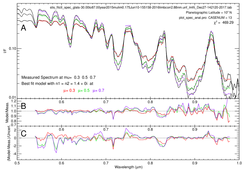
Figure 16.— Top: Model spectra at three view angle cosines (colored as noted in the legend) compared to the 10^∘ N 2015 STIS spectra (black curves). Middle: Ratio of model to measured spectra. Bottom: Difference between model and measured spectra divided by expected uncertainty. The aerosol model used the baseline 2-cloud model, except that $m2\_nr$ was fixed at a value of 1.4. Best fit parameter values are given in Table 6. Note the significant discrepancies at short wavelength continuum peaks, near 740 nm, and within the critical region near 830 nm which is most sensitive to the methane to hydrogen ratio. Better fits were obtained with $m2\_nr$ allowed to adjust as part of the fitting process.

Table 6Preliminary fits to the 540-900 nm part of 2015 STIS 10^∘ N spectra.

Parameter	Value	Value for LP soln.	Value for SP soln.
Name	$m2\_nr$ fixed at 1.4	with $m2\_nr$ fitted	with $m2\_nr$ fitted
$m1\_od$ at $\lambda$ = 0.5 $\mu$m	0.046$\pm$ 0.01	0.050$\pm$ 0.01	0.048$\pm$ 0.01
$m2\_od$ at $\lambda$ = 0.5 $\mu$m	5.155$\pm$ 0.46	7.536$\pm$ 1.42	2.437$\pm$ 0.24
$m2\_pt$ (bar)	1.149$\pm$ 0.04	1.054$\pm$ 0.04	0.962$\pm$ 0.04
$m2\_pb$ (bar)	4.137$\pm$ 0.25	4.102$\pm$ 0.25	3.696$\pm$ 0.22
$m2\_r$ ($\mu$m)	0.382$\pm$ 0.03	1.918$\pm$ 0.33	0.235$\pm$ 0.03
$m2\_nr$	1.400	1.184$\pm$ 0.02	1.828$\pm$ 0.09
$\alpha_{0}$ (%)	1.270$\pm$ 0.05	1.380$\pm$ 0.07	1.900$\pm$ 0.13
$ch4rhc$	0.986$\pm$ 0.13	1.200$\pm$ 0.15	1.200$\pm$ 0.15
$\chi^{2}$	469.29	434.53	371.03
$\chi^{2}$ /NF	1.16	1.07	0.91

NOTES: In the last two columns LP soln. denotes large particle solution and SP soln. denotes small particle solution. The $\chi^{2}$ values given here are based on fitting points spaced 3.2 nm apart.

9.2. Fitting the 730–900 nm region

Our next step was to concentrate on the spectral region where the ratio of methane to hydrogen is best constrained, i.e. the 730–900 nm region. As shown if Fig. 1, the short-wavelength side is free of CIA and sensitive to the deep methane mixing ratio, while the middle region from about 810 to 835 nm is strongly affected by hydrogen CIA, and the long-wavelength side of the region is sensitive to the methane mixing ratio at pressure less than 1 bar. By using this entire region we expect to obtain good constraints on both the ratio of methane to hydrogen as well as on the vertical cloud structure. Results from fitting this region should not be strongly affected by wavelength-dependent particle properties, given the relative modest spectral range we are considering here. If the assumption of Mie scattering over this limited range is seriously flawed, that should show up in an inability to get high quality fits. This relatively narrow spectral range also weakens constraints on particle size, as might be expected.

9.2.1 Effects of different aerosol models

We were somewhat surprised to find that the kind of aerosol model chosen to fit the observations has a significant effect on the derived vertical and latitudinal distribution of methane. To investigate these effects we did model fits at two key latitudes: 10^∘N and 60^∘N. From more detailed latitudinal profiles discussed later, we know that the apparent methane mixing ratio peaks near 10^∘ N and is approaching its polar minimum near 60^∘ N. These are also two latitudes for which 2012 and 2015 observations provide good samples at the three view angle cosines we selected.

9.2.2 Fitting the spherical particle 2-cloud model assuming a uniform CH₄ distribution.

We first consider a methane vertical distribution that has a constant mixing ratio from the deep atmosphere to the condensation level. Above that level (at lower pressures) we assume a drop in relative humidity to an adjustable fraction of the saturation vapor pressure, and from there to the tropopause we interpolate from the above cloud value to the tropopause minimum as described in Section 8.2. The key parameters describing the methane distribution are then the above cloud relative humidity and the deep mixing ratio.

We first consider a simple aerosol model in which the tropospheric contribution is characterized by an adjustable optical depth and a single layer of spherical particles bounded by top and bottom pressures and uniformly mixed with the gas. We assume initially that these particles scatter light conservatively, but allow the real refractive index to be constrained by the spectral observations.

The results of this series of fits for both 2015 and 2012 observations are given in Table 7 where small particle solutions are given in the first four rows and large-particle solutions in the remaining four rows. The model spectra are compared to the observations in Fig. 17. These fits do achieve their intended result of providing more precise constraints on the above-cloud methane humidity, which is high at 10^∘N and about 50% of those levels at 60^∘ N. The temporal change between 2012 and 2015 in the effective methane mixing ratios is very small and well within uncertainty limits. The low latitude values of 3.14$\pm$0.45% and 3.16$\pm$0.50% are consistent with no change, as are the 60^∘N values, which are 0.99$\pm$0.08% and 0.93$\pm$0.08%, for 2015 and 2012 respectively. The factors by which the effective methane mixing ratio declines with latitude are 3.17 and 3.40 for 2015 and 2012 respectively.

Table 7Single tropospheric Mie layer fits to 10^∘N and 60^∘N STIS 730 - 900 nm spectra.

Lat.	$m1\_od$		$m2\_pt$	$m2\_pb$	$m2\_r$		$\alpha_{0}$
(∘)	$\times$100	$m2\_od$	(bar)	(bar)	($\mu$m)	$m2\_nr$	(%)	$ch4rhc$	$\chi^{2}$	YR
10	2.8$\pm$0.8	3.07$\pm$0.9	1.13$\pm$0.04	2.46$\pm$0.22	0.34$\pm$0.10	1.55$\pm$0.16	3.14$\pm$0.45	0.68$\pm$0.13	148.39	2015
60	0.1$\pm$70.7	1.45$\pm$0.3	1.02$\pm$0.02	2.53$\pm$0.13	0.25$\pm$0.09	1.86$\pm$0.30	0.99$\pm$0.08	0.31$\pm$0.18	248.62	2015
10	3.0$\pm$0.7	2.52$\pm$0.6	1.07$\pm$0.04	2.37$\pm$0.20	0.25$\pm$0.09	1.74$\pm$0.26	3.16$\pm$0.50	0.95$\pm$0.16	192.65	2012
60	2.2$\pm$1.6	1.10$\pm$0.2	1.02$\pm$0.04	2.22$\pm$0.13	0.24$\pm$0.07	1.81$\pm$0.25	0.93$\pm$0.08	0.42$\pm$0.20	196.02	2012
10	2.8$\pm$0.8	4.95$\pm$1.4	1.11$\pm$0.04	2.69$\pm$0.19	1.09$\pm$0.48	1.28$\pm$0.07	2.69$\pm$0.28	0.67$\pm$0.14	140.80	2015
60	0.8$\pm$4.5	4.28$\pm$1.1	1.07$\pm$0.03	2.96$\pm$0.16	1.75$\pm$0.52	1.23$\pm$0.05	0.81$\pm$0.05	0.39$\pm$0.24	256.71	2015
10	2.8$\pm$0.7	6.09$\pm$1.9	1.09$\pm$0.04	2.67$\pm$0.19	1.54$\pm$0.58	1.23$\pm$0.06	2.56$\pm$0.26	0.88$\pm$0.16	196.26	2012
60	3.3$\pm$1.5	3.21$\pm$0.8	1.08$\pm$0.04	2.51$\pm$0.14	1.44$\pm$0.53	1.22$\pm$0.05	0.74$\pm$0.05	0.56$\pm$0.26	192.54	2012

NOTE: The optical depths are given for a wavelength of 0.5 $\mu$m. These fits used 318 points of comparison and fit 8 parameters, for a nominal value of NF=310, for which the normalized $\chi^{2}$ /NF ranged from 0.48 to 0.802.

For these fits, the refractive index results for the small-particle solution have a weighted average for both latitudes and both years of 1.68$\pm$0.11, which is much closer to the 1.55 value expected for H₂S, although the 60^∘N values exceed that value by slightly more than their uncertainties. Perhaps this is an indication of a cloud composition difference between the two latitudes. A quite different result is obtained for the large-particle fit. In this case the average index is 1.23$\pm$0.03, which is lower than that of any of the candidate substances, and the individual values don’t vary much from low to high latitudes, or between 2012 and 2015.

The various determinations of the pressure boundaries of the main tropospheric cloud layer are very similar for both years, both latitudes, and both particle-size solutions, extending from a base near 2.5 bars to a top near 1.1 bar. The optical depths do differ substantially between large and small particle solutions because the larger particles are more forward scattering and have a lower refractive index, both differences reducing the back-scattering efficiency of the particles, requiring increased optical depth to make up for the losses.

These results explain the brightening of the polar region at pseudo-continuum wavelengths between 2012 and 2015. To understand how influential these various parameters are on the observed spectrum, we computed logarithmic spectral derivatives (Fig. 18). These have the useful property of showing the fractional changes in the spectrum produced by fractional changes in the various parameters used to model it. For the small particle solution we see that between 2012 and 2015 m2_od increased by 32% at 60^∘ N, providing the main driver for the increase. According to Fig. 7, near 750 nm the I/F increased by about 20%, and according to the derivative spectra in Fig. 18, the optical depth increase would account for about 11%, while the increase in refractive index by just 2.8% would increase the I/F by an additional 10%, accounting for the 20% total. However, these derivatives were computed for a latitude of 10^∘N; somewhat different derivatives might be found at 60^∘N. A similar increase of 33% is seen in the optical depth derived for the large particle solution, although in this case there is also an increase in particle size by 22%, which would also contribute significantly. Weighting these by respective factors of 0.42 and 0.45 (from Fig. 18) we obtain from just these parameters an I/F increase of about 24%, which is again close to the entire change observed. The small changes in inferred methane mixing ratios are increases of 6% for the small particle solution and about 10% for the large particle solution, which would yield I/F decreases of 1.2% and 1.5% for the small and large particle solutions respectively, both of which are well below uncertainties. The fitting errors at high latitudes, which are most evident in the 0.75-$\mu$m region are highlighted by blue dotted ovals in Fig. 17.

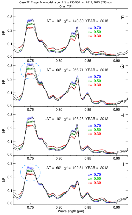
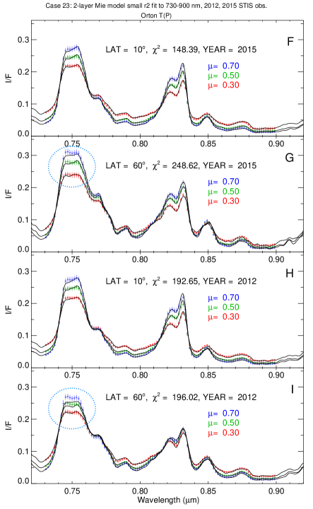
Figure 17.— Comparison of observed spectra (curves) with model fits (points) for the large particle solutions (left) and the small particle solutions (right), both using the model parameterization defined in Table 7. Fits to 2015 STIS observations are shown in the top pair of panels and fits to 2012 observations in the bottom pair of panels. Blue dotted ovals identify regions of high-latitude fitting errors, which can be greatly reduced by using a non-uniform vertical distribution of methane.

Figure 18.— Derivative spectra for uniform mixing ratio models evaluated for the large-particle solution (Left group) and small particle solution (Right group). In each group we show I/F model spectrum (A) and derivatives of fractional changes in I/F with respect to fractional changes in parameters $m1\_od$ (B), $m2\_pb$ (C), $m2\_pt$ (D), $m2\_od$ (E), $m2\_r$ (F), $m2\_nr$ (G), $ch4v0\equiv\alpha_{0}$ (H) and $ch4rhc$ (I). All the derivative panels are scaled the same, except for panel B, which has been expanded by a factor of 4, and panel G, which has been compressed by a factor of 5 because of their unusually small and large effects, respectively, on the I/F spectrum. In panels F and G, the dotted curve represents a version of the $m2\_od$ derivative spectrum scaled to match the lower features of the $m2\_r$ and $m2\_nr$ derivative spectra respectively, to illustrate their strong correlations but resolvable differences.

9.2.3 Fitting the 2-cloud non-spherical model assuming a uniform CH₄ distribution.

We next consider fits in which the main tropospheric layer consists of a single particle type characterized by the simplest possible Henyey-Greenstein function, which is a one-term version of Eq. 8.4.3 characterized by a single asymmetry parameter. The vertical structure parameterization and stratospheric haze layer parameterization are both unchanged from the spherical particle example used in the previous section. Because some wavelength dependence is required, we introduce a wavelength dependent optical depth using a simple linear slope, which is a parameter that is adjusted to optimize the fit. Our model is given by

$$\tau(\lambda)=\tau_{o}\times(1+\mathrm{k_{OD}}\times(\lambda-\lambda_{0}))$$ (5)

where $\lambda_{0}$ is taken to be 800 nm. This also makes $\tau_{o}$ the optical depth at 800 nm. We could also have made the asymmetry parameter wavelength dependent instead of, or in addition to, the optical depth, but found excellent fits without adding any further complexity. We will not be making any claims regarding the true source of wavelength dependence in any case. Our main objective is to find out how this different kind of model affects the methane distribution, and to determine the average asymmetry parameter of these particles. We will also try to infer a single-scattering albedo.

Best-fit parameter values and uncertainties for fits at 10^∘N and 60^∘N for 2012 and 2015 are presented in Table 8. Best-fit model spectral are compared to observations in the left panel of Fig. 19, while fractional derivative spectra are displayed in the right panel. These fits are comparable in quality to the spherical particle fits presented in the previous section, and have the same problem fitting the high-latitude spectra, most notably in the 750-nm region. This region senses more deeply than other parts of this limited spectral range (see Fig. 1), and thus is most likely to be affected by vertical variations in the methane mixing ratio. According to the derivative spectra, an increase in the methane mixing ratio with depth would reduce the I/F in this region, which we would expect to produce a better fit, and we will later show that this does in fact improve the spectral fit in this region.

The methane mixing ratio values for this model average somewhat higher than found for the model using spherical particles, although all are within uncertainty limits for a given latitude, and all results indicate an effective mixing ratio decrease by slightly more than a factor of three from 10^∘N to 60^∘N.

The best-fit asymmetry parameter for this model is generally near 0.4, well below the commonly assumed value of 0.6 for near-IR analysis, which is in part based on an analysis of limb-darkening measurements by Sromovsky and Fry (2008). That analysis predates the significant improvement in methane absorption coefficients seen in the last decade (Sromovsky et al., 2012a) and may no longer be valid. It seems unlikely that this difference is merely a wavelength dependence. For the sizes inferred for spherical particle solutions, the asymmetries either decrease with wavelength (small particle solution), or remain relatively flat (large particle solution). While the asymmetry parameter is highly negatively correlated with the optical depth parameter, these two parameters do have sufficiently different ratios between peaks and valleys to allow them to be independently determined (shown in Fig. 19F). The asymmetry was determined to within about 10% and the optical depth to within slightly better accuracy. The optical depths for this model appears to be considerably lower than for the spherical particle models, which were at a shorter wavelength of 500 nm. If we convert those Mie scattering optical depths to a wavelength of 800 nm, we find that the 0.3-$\mu$m particle optical depth drops from 3.1 to 2.6 and the 1.54 $\mu$m particle optical depth increases from 6.1 to 7.5. Thus, the wavelength difference does not explain the low optical depths of the non-spherical model. It is more likely due to the latter’s more symmetric scattering. The Mie particle models have asymmetries of about 0.68 and 0.87 for the small and large particle solutions respectively, both adjusted to a reference wavelength of 800 nm. The particles of KT2009, which use a DHG phase function, with their adopted values of $g_{1}$ = 0.7 and $g_{2}$= -0.3, yield an asymmetry of 0.6, which is much closer to that of our small particle solution for spherical particles, and much larger than our HG particle solutions. We tried to find an HG solution with larger asymmetry by using a first guess with $g$ = 0.63, but the regression again converged on $g$ = 0.43. It is apparently the case that very different scattering properties can lead to very nearly the same fit quality, but very different optical depths and asymmetry parameters. At phase angles near zero, there is a considerable ambiguity between more forward scattering particles with larger optical depths and more backward scattering particles with smaller optical depths.

Table 8Single tropospheric HG layer fits to 10^∘N and 60^∘N STIS spectra.

Lat.	$m1\_od$		$hg2\_pt$	$hg2\_pb$		$hg2\_kod$	$\alpha_{0}$
(∘)	$\times$100	$hg2\_od$	(bar)	(bar)	$hg2\_g$	(/$\mu$m )	(%)	$ch4rhc$	$\chi^{2}$	YR
10	2.6$\pm$0.5	1.58$\pm$0.13	1.13$\pm$0.03	2.33$\pm$0.15	0.43$\pm$0.04	-2.23$\pm$0.4	3.48$\pm$0.45	0.65$\pm$0.08	151.51	2015
60	0.0$\pm$0.0	0.97$\pm$0.05	1.01$\pm$0.02	2.53$\pm$0.12	0.26$\pm$0.02	-3.18$\pm$0.3	0.97$\pm$0.06	0.31$\pm$0.03	252.65	2015
10	2.7$\pm$0.5	1.57$\pm$0.14	1.07$\pm$0.03	2.47$\pm$0.17	0.42$\pm$0.04	-1.91$\pm$0.4	2.85$\pm$0.32	0.87$\pm$0.12	192.22	2012
60	2.0$\pm$1.2	0.71$\pm$0.06	1.01$\pm$0.02	2.04$\pm$0.08	0.39$\pm$0.04	-3.95$\pm$0.3	1.04$\pm$0.07	0.39$\pm$0.15	193.30	2012

NOTE: The optical depth is for a wavelength of 0.8 microns for $hg2\_od$, and for 0.5 $\mu$m for the stratospheric haze ($m1\_od$). These fits used 318 points of comparison and fit 8 parameters, for a nominal value of NF=310, for which the normalized $\chi^{2}$ /NF ranged from 0.48 to 0.802.

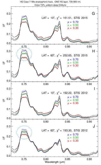
Figure 19.— Left: HG Model spectra compared to observations at 10^∘N and 60^∘N for 2012 (bottom pair) and 2015 observations (top pair), with models plotted as points with error bars. Right: Derivative spectra showing the ratio of a fractional change in I/F to the fractional change in the parameter producing the change (here $ch4v0\equiv\alpha_{0}$). The dotted curve in panel F of the derivative group is an inverted plot of the curve in panel E, with minima scaled to match the solid curves. Note that the maxima do not match, making them distinguishable.

The best-fit optical depth slope parameter $hg2\_kod$ is negative, as generally expected, and is around -2/$\mu$m at 10^∘N but -3.2 /$\mu$m to -4/$\mu$m at 60^∘N. A spherical particle of radius 0.3 $\mu$m and real index 1.4 would have a slope of about -2.4/$\mu$m. For spherical particles, some of the wavelength dependence in scattering is provided by wavelength dependence in the phase function. This suggests a possible decrease in particle size at high latitudes.

There is better agreement between the HG solution and the small particle Mie solutions regarding other parameters, including pressure boundaries, methane mixing ratios and above cloud humidities. Thus, the preponderance of evidence suggests that the cloud particles can be roughly approximated by the small particle Mie solutions, which is the solution type we will use to investigate the latitude dependent characteristics in more detail.

9.2.4 Latitude-dependent fits

To illustrate the latitude dependence of the effective methane mixing ratio and the inferred aerosol distribution we selected the simple 2-layer model using a compact stratospheric haze and an extended diffuse layer of spherical tropospheric particles, characterized by Mie scattering parameters of radius and refractive index. We also chose the small-radius solution set because of their high quality fits and relative consistency between 2012 and 2015, as well as their better agreement with HG fits as noted in the previous section. Other models show similar characteristics, except that they contain more variation between years, as can be surmised from the table of fit parameters from fits at 10^∘N and 60^∘N, shown in Table 7 for large Mie particle fits and in Table 8 for HG model fits. We assumed a methane profile that has a vertically uniform fitted deep mixing ratio, a fitted relative humidity immediately above the condensation level, a minimum relative humidity of 30%, with linear interpolation filling in values between the condensation level and the tropopause. Above the tropopause we assumed a mixing ratio equal to the tropopause value. From fitting spectra every 10^∘ of latitude for both 2012 and 2015 observations we obtained the best-fit parameters and their formal uncertainties given in Table 9. The parameters are also plotted in Fig. 20, where panels A-E display the fit parameter values and their estimate errors, and panels F-I display samples of model and observed spectra for 10^∘ N and 60^∘ N for 2015 (F and G) and 2012 (H and I).

[!t] Lat. $m1\_od$ $m2\_pt$ $m2\_pb$ $m2\_r$ $\alpha_{0}$ (^∘) $\times$100 $m2\_od$ (bar) (bar) ($\mu$m ) $m2\_nr$ (%) $ch4rhc$ $\chi^{2}$ YR -10 2.4$\pm$0.8 3.60$\pm$1.37 1.09$\pm$0.04 2.66$\pm$0.22 0.22$\pm$0.09 1.65$\pm$0.31 2.93$\pm$0.37 0.75$\pm$0.14 180.61 2015 0 4.5$\pm$0.8 2.52$\pm$0.67 1.07$\pm$0.04 2.55$\pm$0.20 0.25$\pm$0.08 1.72$\pm$0.24 2.69$\pm$0.38 0.61$\pm$0.14 137.93 2015 10 2.8$\pm$0.8 3.07$\pm$0.88 1.13$\pm$0.04 2.46$\pm$0.22 0.34$\pm$0.10 1.55$\pm$0.16 3.14$\pm$0.45 0.68$\pm$0.13 148.39 2015 20 2.8$\pm$0.7 1.99$\pm$0.58 1.08$\pm$0.05 2.55$\pm$0.22 0.28$\pm$0.11 1.75$\pm$0.29 2.85$\pm$0.39 0.97$\pm$0.18 170.32 2015 30 3.8$\pm$0.8 1.48$\pm$0.49 1.06$\pm$0.05 2.60$\pm$0.20 0.27$\pm$0.13 1.81$\pm$0.36 2.10$\pm$0.24 0.88$\pm$0.19 170.86 2015 40 2.8$\pm$0.9 1.41$\pm$0.36 1.01$\pm$0.04 2.65$\pm$0.17 0.27$\pm$0.10 1.79$\pm$0.28 1.41$\pm$0.12 0.75$\pm$0.20 205.54 2015 50 2.4$\pm$1.1 1.25$\pm$0.42 1.01$\pm$0.04 2.51$\pm$0.14 0.26$\pm$0.16 1.88$\pm$0.46 1.13$\pm$0.09 0.76$\pm$0.22 266.49 2015 60 0.1$\pm$70.7 1.45$\pm$0.29 1.02$\pm$0.02 2.53$\pm$0.13 0.25$\pm$0.09 1.86$\pm$0.30 0.99$\pm$0.08 0.31$\pm$0.18 248.62 2015 70 0.4$\pm$13.4 1.49$\pm$0.26 1.01$\pm$0.03 2.71$\pm$0.14 0.23$\pm$0.09 1.90$\pm$0.33 0.88$\pm$0.07 0.36$\pm$0.21 278.56 2015 -20 1.4$\pm$0.7 3.14$\pm$1.19 1.11$\pm$0.04 2.71$\pm$0.22 0.24$\pm$0.09 1.66$\pm$0.29 2.87$\pm$0.36 0.77$\pm$0.13 137.66 2012 -10 4.4$\pm$0.7 3.28$\pm$1.22 1.04$\pm$0.05 2.77$\pm$0.23 0.25$\pm$0.09 1.64$\pm$0.27 2.63$\pm$0.32 1.17$\pm$0.21 147.88 2012 0 4.7$\pm$0.8 2.51$\pm$0.64 1.08$\pm$0.04 2.56$\pm$0.21 0.25$\pm$0.08 1.73$\pm$0.24 2.69$\pm$0.37 0.58$\pm$0.12 150.60 2012 10 3.0$\pm$0.7 2.52$\pm$0.64 1.07$\pm$0.04 2.37$\pm$0.20 0.25$\pm$0.09 1.74$\pm$0.26 3.16$\pm$0.50 0.95$\pm$0.16 192.65 2012 20 2.6$\pm$0.7 3.42$\pm$1.14 1.06$\pm$0.05 2.63$\pm$0.21 0.27$\pm$0.08 1.62$\pm$0.22 2.65$\pm$0.33 0.95$\pm$0.17 197.68 2012 30 2.7$\pm$0.7 1.98$\pm$0.51 1.02$\pm$0.05 2.69$\pm$0.19 0.26$\pm$0.08 1.74$\pm$0.24 1.99$\pm$0.21 0.89$\pm$0.18 149.64 2012 40 2.8$\pm$1.0 2.07$\pm$0.51 1.06$\pm$0.04 2.42$\pm$0.15 0.32$\pm$0.08 1.57$\pm$0.14 1.29$\pm$0.12 0.62$\pm$0.18 255.27 2012 50 0.4$\pm$1.55 1.94$\pm$0.39 1.07$\pm$0.03 2.47$\pm$0.13 0.32$\pm$0.06 1.59$\pm$0.12 1.03$\pm$0.08 0.30$\pm$0.17 191.32 2012 60 2.2$\pm$1.6 1.10$\pm$0.23 1.02$\pm$0.04 2.22$\pm$0.13 0.24$\pm$0.07 1.81$\pm$0.25 0.93$\pm$0.08 0.42$\pm$0.20 196.02 2012 70 1.8$\pm$2.1 1.00$\pm$0.12 1.01$\pm$0.03 2.23$\pm$0.12 0.19$\pm$0.09 1.97$\pm$0.36 0.97$\pm$0.08 0.29$\pm$0.19 235.18 2012 NOTE: The optical depths are for a wavelength of 0.5 $\mu$m. These fits used 318 points of comparison and fit 8 parameters, for a nominal value of NF=310, for which the normalized $\chi^{2}$ /NF ranged from 0.44 to 0.90.

Table 9Single tropospheric Mie layer fits to the 730-900 nm spectra as a function of latitude assuming vertically uniform CH₄ below the condensation level.

Most of the model parameters are found to have only weak variations with latitude. The top pressure of the sole tropospheric cloud layer is surprisingly invariant from low to high latitudes as well as from 2012 to 2013, even though there are substantial variations in optical depth between years as well as with latitude. This boundary pressure is also very well constrained by the observations. The bottom pressure of this cloud is more variable, but its variation is not much more than its uncertainty which is much larger than that of the cloud top pressure. The larger uncertainty is consistent with the derivative spectra given in Fig. 18, which shows that, compared to the top pressure, the bottom pressure has a smaller fractional effect on the I/F spectrum for a given fractional change in pressure.

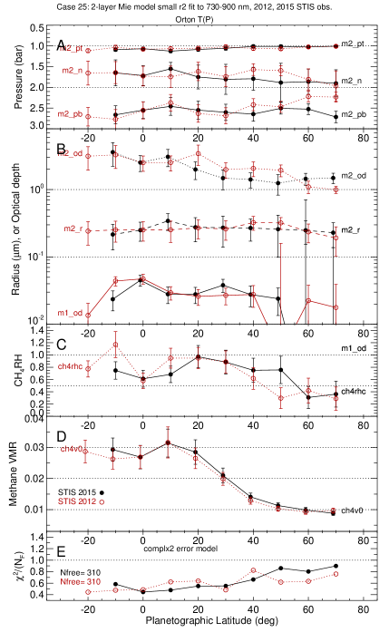
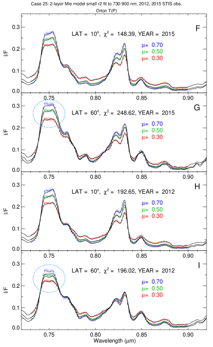
Figure 20.— Left: Single tropospheric Mie model fits as a function of latitude under the assumption that the methane VMR is constant for pressures exceeding the condensation level. Parameter values are also given in Table 9. Right: sample spectra, with blue dotted ovals identifying regions of larger I/F errors.

The most prominent latitudinally varying parameter is the effective deep methane mixing ratio, which attains a low-latitude maximum of about 3.15%, dropping to about 2% by 30^∘ N, reaching a high-latitude value of about 1% at between 50^∘N and 60^∘N. Close behind, is the variation in methane humidity above the condensation level, which was found to be 60-100% at low latitudes, declining to about 30-40% for regions poleward of 50^∘ N. This decline towards the north pole is also seen in other model types as well.

There is also close agreement, for this model, between between 2012 and 2015 results for both the extremes in the methane mixing ratio and in its latitudinal variation. The slight dip at the equator is also present in results for both years, as is the peak at 10^∘N. The agreement of the 2012 and 2015 methane profiles (on both the deep mixing ratio and the above cloud humidity) is close enough that we must look elsewhere to explain the brightening of the polar region between 2012 and 2015. The most likely aerosol change responsible for the polar brightening is the increase in the bottom cloud layer optical depth ($m2\_od$) by about 60% at latitudes north of 50^∘, a factor already discussed in Section 9.2.2. However, because multiple aerosol parameters differ between 2012 and 2015, it is useful to show that the combined effect of layer m2 parameter changes does indeed result in the increased scattering that produced the observed brightness increase. This was done by starting with the model spectrum for 2012 and computed a new model spectrum in which only the layer-m2 parameters were changed to match those of 2015, leaving other parameters unchanged. We also computed the spectrum change when only the optical depth of the m2 layer was changed to the 2015 value. We did this at latitudes of 50^∘N, 60^∘N, and 70^∘N. The results are summarized in the following figures. The left-hand figure provides a sample spectral view at 60^∘ N. It shows the measured spectral difference between 2012 and 2015 as a shaded curve, with shading range indicating uncertainties. Also shown are the difference in model fits (+), the difference due only to layer m2 differences ($\times$), and the difference due only to the change in optical depth (o). The right hand plot displays the latitude dependence for two pseudo-continuum wavelengths. Again are shown the measured differences (shaded curves), the model difference ($\times$), and the brightness change due only to layer m2 (+). This figure shows that layer m2 is clearly responsible for the vast majority of the brightness increase between 2012 and 2015, but changes in the m2 layer optical depth are only responsible for about half of the total scattering increases of that layer (as in the left hand plot), except at 50^∘N, where even though the optical depth decreased, the layer still brightened because of changes in particle size and refractive index).

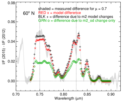
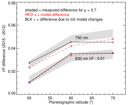
Figure 21.— Left: spectral difference at 60^∘N between 2012 and 2015 observations at a zenith angle cosine of 0.7 (shaded curve) compared to all model differences ($\times$), to those contributed only by layer m2 (+), and to those due only to the m2 optical depth change (o). Right: latitudinal variation of observed temporal differences at 750 nm (upper shaded curve) and 830 nm (lower shaded curve offset by 0.01), compared to total model differences ($\times$) and differences due to all changes in layer m2 only (+). This shows that increased scattering by layer m2 is primarily responsible for the observed brightening of the polar region between 2012 and 2015.

At low latitudes, the fit quality for both years is better than expected from our uncertainty estimates, but fit quality decreases significantly at high northern latitudes, especially for the 2015 fits, which have increased aerosol scattering. The high latitude fitting problem is most obvious just short of 750 nm, as shown in panels G and I of Fig. 20, where the model values exceed the measured values (note the encircled regions). This problem can be greatly reduced by using an altered vertical profile of methane, as discussed in Section 9.3.

9.2.5 Summary of uniform methane results

Both spherical particle and HG models for the upper tropospheric layer lead to declining effective methane volume mixing ratios with latitude by similar factors, but are in some disagreement with respect to magnitudes, as shown in greater detail in Fig. 22. The more detailed latitudinal fit results in Fig. 20 for the small-particle solution, show that the effective methane mixing ratio peaks near 10^∘ N in both years, has a local minimum at the equator and declines with latitude by more than a factor of two by 50-60^∘ N. For each year, the two aerosol models lead to similar shapes, and in the 50-70^∘ range the two models agree that there is a crossover in which the 2015 vmr declines from 50^∘ to 70^∘, while the 2012 vmr rises slightly over the same interval.

The fitted values of the methane relative humidity just above the condensation level, shown in Fig. 22B, have considerable uncertainty. But both results indicate a peak near 20^∘ N, a clear local minimum near the equator, and a strong decline towards the north pole. This is suggestive of rising motions near 20^∘ and descending motions near the equator and poles, with the latter being more significant.

Figure 22.— Effective deep methane VMR for different aerosol model parameterizations at 10^∘ N (A) and 60^∘ N (B). Vertical lines show unweighted mean values for 2015 (dashed) and 2012 (dotted).

9.2.6 The effects of particle absorption on derived methane amounts

The modeling results presented so far are for conservative particles ($\varpi$ = 1.0). Particles that absorb some fraction of the incident light will act to darken the atmosphere and reduce the amount of methane needed to fit the spectrum. This is true even if the particles are not distributed vertically in the same fashion as methane, and even though they lack the band structure of methane. The aerosol optical depths and derived pressure locations of the layers are also altered. To investigate the magnitude of these effects we did fits of the 2 Mie layer model to the 2015 STIS observations, under the assumption of vertically uniform methane, but with the imaginary index of the tropospheric layer increased from zero to 0.0049, which, for a 0.3-$\mu$m radius particle with a real refractive index of 1.8 corresponds to a decrease in single scattering albedo at 0.8 $\mu$m from $\varpi$ = 1.0 to $\varpi\approx$ 0.979. This amount of absorption in the 730 to 900 nm part of the spectrum, makes it possible to fit the entire spectrum (down to 540 nm) if the particles are assumed to be conservative at the shorter wavelengths (see Sec. 9.4 for more information). Table 10 shows that adding this amount of absorption changes the layer-2 top pressures by just fractions of a percent, while increasing the bottom pressures by 18-22%. The optical depth of the layer changes in less consistent directions. If the particle’s refractive index and size did not change much, then an increase in optical depth would be required to make up for the lower single-scattering albedo produced by absorption. However, the optical depth is seen to decrease at 10^∘N, where $m2\_nr$ has increased by almost 10% (and $m2\_nr$ - 1 by 28%), increasing the scattering efficiency substantially. For 60^∘N, the changes in $m2\_r$, $m2\_nr$, and $m2\_od$ are all substantially smaller. Most importantly, the effective deep methane mixing ratio is decreased by 3% at 10^∘N and 7% at 60^∘N, which suggests that a fair approximation of the latitudinal profile for absorbing cloud particles can be obtained by scaling the profile we derived from conservative scattering. Whether the cloud particles are actually absorbing in the 730-900 nm region remains to be determined.

For the large-particle solution, we made a similar comparison, but just for 10^∘ N and for 2012. In this case the increase of imaginary index needed to adjust the wavelength dependence (as described above for the small-particle solution) is only from 0 to 6.2$\times 10^{-4}$, which decreases the single-scattering albedo for a 1.535 $\mu$m particle with real index 1.225 to $\varpi=$ 0.990 at 0.8 $\mu$m. Although this seems like a small change, it produces a 50% increase in optical depth, a 56% increase in the cloud bottom pressure, and a 10.6% decrease in the best-fit methane mixing ratio, as shown in Table 11. For non-spherical particles in which wavelength-dependent optical depths or wavelength dependent phase functions might be used to adjust the wavelength dependent I/F spectrum, there may be no need for absorbing particles, in which case the somewhat higher methane mixing ratios may apply.

Table 10Changes in small-particle best-fit parameter values derived from the STIS 2015 observations, as a result of adding absorption to aerosol layer 2 by increasing $m2\_ni$ from 0.0 to 0.005.

	10∘N Latitude			60∘N Latitude
Parameter	Value	Value		Value	Value
Name	$m2\_ni$ = 0	$m2\_ni$ = 0.005	Difference	$m2\_ni$ = 0	$m2\_ni$ = 0.005	Difference
$m2\_od$	3.084	2.864	-7.15%	1.445	1.482	2.54%
$m2\_pt$ (bar)	1.126	1.127	0.14%	1.023	1.032	0.87%
$m2\_pb$ (bar)	2.450	2.993	22.12%	2.519	2.968	17.79%
$m2\_r$ ($\mu$m)	0.342	0.307	-10.16%	0.248	0.256	2.89%
$m2\_nr$	1.554	1.706	9.77%	1.862	1.900	2.05%
$\alpha_{0}$ $\times$100	3.160	3.060	-3.16%	0.989	0.916	-7.38%
$ch4rhc$	0.687	0.701	2.04%	0.318	0.355	11.64%
$\chi^{2}$	148.03	148.85	0.55%	248.29	246.28	-0.81%

Table 11Changes in large-particle best-fit parameter values derived from the STIS 2015 observations, as a result of adding absorption to aerosol layer 2 by increasing $m2\_ni$ from zero to 6.2$\times 10^{-4}$.

	10∘N Latitude
Parameter	Value	Value
Name	$m2\_ni$ = 0	$m2\_ni$ = 6.2$\times 10^{-4}$	Difference
$m2\_od$	6.088	9.124	49.87%
$m2\_pt$ (bar)	1.094	1.112	1.64%
$m2\_pb$ (bar)	2.675	4.183	56.39%
$m2\_r$ ($\mu$m)	1.535	1.597	4.01%
$m2\_nr$	1.225	1.243	1.42%
$\alpha_{0}$ $\times$100	2.560	2.290	-10.55%
$ch4rhc$	0.879	0.877	-0.23%
$\chi^{2}$	196.26	193.13	-1.59%

9.3. Fitting latitude-dependent vertically non-uniform methane depletion models

9.3.1 Alternative models of vertically varying methane

The fits discussed in previous sections have assumed that the methane profile is vertically uniform from the bottom of our model atmosphere all the way up to the methane condensation level. We have already noted problems with those fits in the 750 nm region of the spectrum, which suggest that the methane mixing ratio likely increases with depth at high latitudes. There are also independent physical arguments suggesting the same characteristic. Sromovsky et al. (2011) pointed out that extending the very low high latitude mixing ratios to great depths would result in horizontal density gradients over great depths. As a consequence of geostrophic and hydrostatic balance, these gradients would lead to vertical wind shears (Sun et al., 1991). This would result in an enormous wind difference with latitude at the visible cloud level, which would be inconsistent with the observed winds of Uranus. Thus, we would expect that the polar depletion would be a relatively shallow effect, as we have inferred from our previous work (Karkoschka and Tomasko, 2009; Sromovsky et al., 2011, 2014). As indicated by KT2009, the 2002 spectral observations did not require that methane depletions extend to great depths, and Sromovsky et al. (2011) showed that shallow depletions were preferred by the 2002 spectra. This was further supported by de Kleer et al. (2015), who used our descended profile parameterization, fixed the shape parameter at $vx=2$, and constrained the depth parameter vs latitude using H band spectra. They found a clear latitude trend, with a low-latitude value of 1.7$\pm$0.2 bars, increasing to 3.2$\pm$1 bars in the 40–50^∘N band, and as deep as 26${}^{+11}_{-18}$ bars in the 60–70^∘N band, although at that extreme value the depth parameter is constrained more by the shape of the profile at much lower pressures than by any direct sensing of sunlight reflected from the 26-bar level.

From the previous discussion, we expect a reasonable physical model has some pressure value $P_{d}$ for which the methane mixing ratio is independent of latitude for $P>P_{d}$, but allows a decline in mixing ratio with latitude for $P<P_{d}$. We assume that the highest mixing ratio we observe at low latitudes (which turns out to be at 10^∘N) is representative of the deep mixing ratio and assume all of the variation with latitude is a depletion relative to that level. Here we describe the results of fitting two alternative vertically varying depletion models: the descended profile model described in Fig. 14A and Eq. 8.3, and the step function depletion described in Fig. 14B. Both options result in improved fit quality at high latitudes, with depletions confined to the upper troposphere.

We first consider the stepped depletion model shown in Fig. 14B because it is easier to constrain its bottom boundary at all latitudes. A more detailed look at the 60^∘N spectrum from 2012 in comparison with a model fit using a vertically uniform methane mixing ratio is shown in Fig. 23A-C, while our best fit model for the stepped methane profile is displayed in Fig. 23D-F. Here we assume that the deep mixing ratio is equal to the 10^∘N best fit uniform VMR value of 3.14%, and optimize the depleted mixing ratio $\alpha_{1}$ and the depth of the depletion $P_{d}$ to minimize $\chi^{2}$. The result is seen to be a substantial improvement of the fit in the 750-nm region, with minor improvements in other areas, with an overall significant reduction in $\chi^{2}$ for the entire fit from 196.02 to 160.72. The fact that the difference plots show strong features in the vicinity of large slopes in the spectrum, particularly at 0.88 $\mu$m, suggests that there may be a slight error in the STIS wavelength scale. If we move the observed spectrum just 0.24 nm towards shorter wavelengths, these $\chi^{2}$ values can be reduced to 170.02 and 137.93 respectively. (Although the STIS wavelengths are very accurate up to 653 nm because of the availability of numerous Fraunhofer calibration lines, longer wavelengths require extrapolation that allows errors of this size.) The best fit values for the methane profile parameters are $ch4vx$ = 0.73$\pm$0.08% and $P_{d}$ = 3.0${}^{+3.5}_{-1.5}$ bars. The methane value is a little below the 0.93$\pm$0.08% for the uniform mixing ratio model, as expected. The methane relative humidity above the condensation level was found to be 95$\pm$16% for the uniform case and 67$\pm$32% for the upper tropospheric depletion case. The uncertainty in the depth of depletion ($P_{d}$) is much larger on the high side because the sensitivity to that parameter decreases with depth.

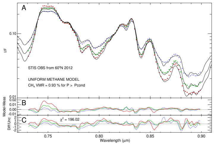
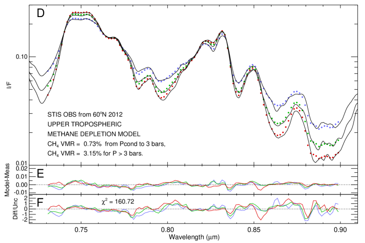
Figure 23.— Detailed comparison of 60^∘N 2012 STIS observations with best-fit model spectra assuming vertically uniform methane VMR (A-C) and with model calculations assuming a step-function change in methane VMR (D-F), where observations are plotted as continuous curves and models as colored points, using red, green, and blue for $\mu$ values of 0.3, 0.5, and 0.7 respectively. Below each spectral plot are plots of model minus observation (B and E) and the same difference divided the expected uncertainty (C and F). Methane profiles are described in the legends.

We also tried fits with the descended depletion function described in Fig. 14A and Eq. 8.3, which is defined by a shape parameter $vx$ and a depth parameter $P_{d}$. We found the depth parameter difficult to constrain because the rate of change of mixing ratio with depth can be come quite small for large depths due to the shape of the function. However, fixing $P_{d}$ at 5 bars, and using just the shape parameter to control the depletion, we obtained a $\chi^{2}$ value of 167.34 and a shape parameter of $vx$ = 1.22$\pm$0.54, fitting the same 2012 60^∘N observation as in Fig. 23. Thus, a descended depletion fit is also viable, and probably a more realistic vertical variation than the step function. The advantage of the step function is that both parameters can be fit without too much difficulty.

9.3.2 Latitude dependent fits with a stepped depletion of methane

Here we describe the results of assuming a stepped depletion of methane, parameterized by one fixed parameter ($\alpha_{0}$, the deep methane VMR, which is set to 0.0315) and two adjustable parameters ($P_{d}$, the pressure at which the step occurs and $\alpha_{1}$, the decreased mixing ratio between that level and the condensation level (which is a function of the decreased methane VMR). In addition to fitting these two parameters, we fit the usual aerosol parameters and the methane relative humidity above the condensation level, resulting in a net increase of one adjustable parameter, for a new total of nine. The best-fit parameter values and their uncertainties are given at 10^∘ latitude intervals for both 2012 and 2015 in Table 12. These are plotted versus latitude in the left column of Fig. 24 and comparisons of model and observed spectra are displayed in the right column.

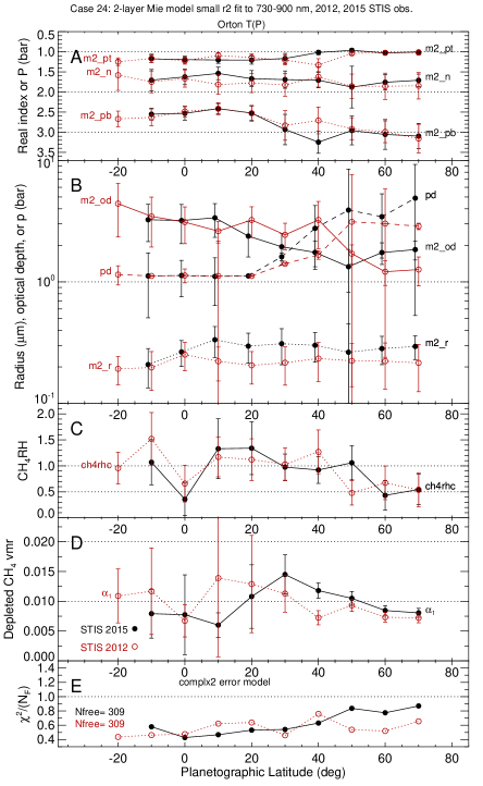
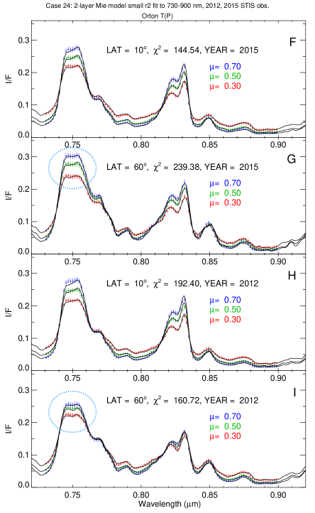
Figure 24.— Stepped depletion model of vertical methane distribution fit to STIS spectra from 2012 and 2015. Conservative cloud model and gas profile parameters for a Mie-scattering haze above a single diffuse Mie-scattering tropospheric layer, assuming a deep mixing ratio of $\alpha_{0}$ = 0.0315, and a methane profile characterized by a pressure depth parameter $P_{d}$ and a depleted mixing ratio $\alpha_{1}$ (defined in Fig. 14) and constrained by spectral observations from 730 nm to 900 nm. The parameter values are in panels A-E, with red (open circle) points displaying results of fitting 2012 STIS observations and black (filled circle) points displaying the results of fitting 2015 observations. Sample comparisons between measured and large-particle model spectra are in panels F-I. Note the great improvement in the high latitude fits near 745 nm, compared to results given in Fig. 20.

The best-fit methane depletion depth parameter values are shown by dashed lines in panel B of Fig. 24 for $P_{d}$ and by dotted lines in panel D for $\alpha_{1}$. At high latitudes the latter is near 0.8%, and increases somewhat at low latitudes, but becomes very uncertain at low latitudes, which is a result of having less and less influence on the spectrum as the depth of the depletion decreases towards the condensation level. As shown in panel D, the depletion depth is in the 3-5 bar range from 70^∘N down to about 50^∘N, and then declines to nearly the condensation level by 20^∘N, and at low latitudes there is almost no depletion. The improvement in fit quality is significant at high latitudes.

Table 12Single tropospheric Mie layer fits to the 730-900 nm spectra as a function of latitude assuming stepped depletion of CH₄ below the condensation level.

Lat.	$m1\_od$		$m2\_pt$	$m2\_pb$	$m2\_r$			$\alpha_{1}$	$P_{d}$
(∘)	$\times$100	$m2\_od$	(bar)	(bar)	($\mu$m )	$m2\_nr$	$ch4rhc$	(%)	(bar)	$\chi^{2}$	YR
-10	3.5$\pm$1.3	3.25$\pm$1.10	1.18$\pm$0.10	2.55$\pm$0.15	0.21$\pm$0.07	1.71$\pm$0.27	1.07$\pm$0.43	0.79$\pm$0.41	1.12$\pm$0.61	178.88	2015
0	3.1$\pm$2.0	3.20$\pm$1.14	1.19$\pm$0.08	2.53$\pm$0.17	0.27$\pm$0.06	1.62$\pm$0.19	0.36$\pm$0.31	0.77$\pm$0.67	1.13$\pm$0.37	132.16	2015
10	4.7$\pm$1.3	3.37$\pm$1.04	1.20$\pm$0.08	2.41$\pm$0.12	0.33$\pm$0.10	1.54$\pm$0.15	1.33$\pm$0.57	0.60$\pm$0.20	1.11$\pm$0.47	144.54	2015
20	3.8$\pm$1.3	2.38$\pm$0.78	1.21$\pm$0.10	2.52$\pm$0.17	0.30$\pm$0.08	1.67$\pm$0.20	1.34$\pm$0.51	1.08$\pm$0.53	1.12$\pm$0.01	164.33	2015
30	4.2$\pm$1.0	1.95$\pm$0.57	1.17$\pm$0.12	2.93$\pm$0.38	0.31$\pm$0.10	1.69$\pm$0.22	0.98$\pm$0.25	1.45$\pm$0.33	1.61$\pm$0.12	167.31	2015
40	3.3$\pm$1.0	1.75$\pm$0.42	1.02$\pm$0.06	3.25$\pm$0.28	0.30$\pm$0.08	1.71$\pm$0.19	0.92$\pm$0.26	1.18$\pm$0.13	2.76$\pm$1.49	194.88	2015
50	3.1$\pm$1.0	1.33$\pm$0.51	0.96$\pm$0.05	2.96$\pm$0.36	0.26$\pm$0.19	1.88$\pm$0.52	1.06$\pm$0.33	1.05$\pm$0.12	3.90$\pm$4.58	258.44	2015
60	0.8$\pm$3.8	1.74$\pm$0.35	1.03$\pm$0.03	3.06$\pm$0.37	0.28$\pm$0.07	1.76$\pm$0.19	0.43$\pm$0.28	0.85$\pm$0.08	3.44$\pm$1.87	239.38	2015
70	1.4$\pm$1.9	1.85$\pm$0.33	1.00$\pm$0.04	3.10$\pm$0.32	0.29$\pm$0.06	1.71$\pm$0.15	0.55$\pm$0.29	0.81$\pm$0.08	4.89$\pm$4.36	268.77	2015
-20	2.0$\pm$1.1	4.41$\pm$2.06	1.25$\pm$0.09	2.67$\pm$0.19	0.19$\pm$0.05	1.58$\pm$0.38	0.96$\pm$0.30	1.09$\pm$0.45	1.15$\pm$0.21	134.90	2012
-10	5.2$\pm$1.1	3.46$\pm$1.53	1.17$\pm$0.11	2.63$\pm$0.21	0.20$\pm$0.07	1.75$\pm$0.27	1.52$\pm$0.51	1.17$\pm$0.73	1.12$\pm$0.01	142.97	2012
0	5.1$\pm$1.5	3.10$\pm$1.04	1.22$\pm$0.09	2.48$\pm$0.13	0.25$\pm$0.07	1.67$\pm$0.22	0.66$\pm$0.35	0.67$\pm$0.27	1.13$\pm$0.15	147.11	2012
10	3.7$\pm$1.1	2.62$\pm$0.53	1.09$\pm$0.08	2.42$\pm$0.15	0.22$\pm$0.07	1.81$\pm$0.24	1.17$\pm$0.38	1.39$\pm$1.32	1.12$\pm$1.05	192.40	2012
20	3.1$\pm$1.1	3.23$\pm$0.92	1.14$\pm$0.09	2.53$\pm$0.20	0.21$\pm$0.06	1.78$\pm$0.24	1.12$\pm$0.40	1.29$\pm$0.82	1.12$\pm$0.01	197.25	2012
30	3.2$\pm$1.0	2.44$\pm$0.60	1.21$\pm$0.12	2.83$\pm$0.37	0.22$\pm$0.08	1.82$\pm$0.28	1.03$\pm$0.32	1.13$\pm$0.31	1.41$\pm$0.03	141.96	2012
40	4.8$\pm$1.1	3.24$\pm$1.36	1.33$\pm$0.16	2.71$\pm$0.33	0.23$\pm$0.08	1.62$\pm$0.25	1.27$\pm$0.42	0.72$\pm$0.12	1.67$\pm$0.14	234.70	2012
50	0.9$\pm$2.1	1.71$\pm$0.31	1.04$\pm$0.03	2.92$\pm$0.28	0.22$\pm$0.09	1.86$\pm$0.30	0.48$\pm$0.23	0.93$\pm$0.10	3.12$\pm$4.50	166.19	2012
60	3.4$\pm$1.4	1.21$\pm$0.28	1.03$\pm$0.06	2.99$\pm$0.27	0.22$\pm$0.09	1.86$\pm$0.33	0.67$\pm$0.32	0.73$\pm$0.08	3.02$\pm$2.78	160.72	2012
70	3.4$\pm$1.7	1.26$\pm$0.34	1.02$\pm$0.06	3.16$\pm$0.36	0.22$\pm$0.09	1.84$\pm$0.33	0.54$\pm$0.33	0.72$\pm$0.08	2.87$\pm$0.17	202.39	2012

NOTE: The optical depth is for a wavelength of 0.5 $\mu$m. These fits used 318 points of comparison and fit 8 parameters, for a nominal value of NF=310, for which the normalized $\chi^{2}$ /NF ranged from 0.426 to 0.87.

In comparison with the uniform methane fit results, we see only minor changes in most of the other parameters. The top pressure of the tropospheric cloud layer is nearly the same for both models, although the stepped depletion model results show a little more variability. The retrieved bottom pressure shows more significant changes. The new results show much closer agreement between years, but more change with respect to latitude, increasing from about 2.5 bars at low latitude to 3 bars at high latitude. The prior results showed no consistent trend with latitude, averaging about 2.7 bars. The optical depth for that layer shows about the same trend with latitude and the same increase at high latitudes between 2012 and 2015. The particle size generally remains between 0.2 and 0.4 $\mu$m for both models, but the descended model fits indicate that particles in the northern hemisphere are about 40% larger in 2015 than in 2012, while the uniform model showed much less difference between years. All these particle size differences are within uncertainties, however. The relative humidity results for methane are roughly similar for the two model types, with higher, near saturation levels at low latitudes and a factor of two decline in the polar region. Both find the methane humidity depressed at the equator, with a slightly sharper decline seen in the descended profile results.

The refractive index results differ a little. For the descended depletion model fits for 2012 and 2013 are in somewhat better agreement than for the uniform model, and do not show as much trending towards slightly higher values at high latitudes.

9.3.3 Latitude dependent fits with descended depletion of methane

Because the descended depletion function approaches the deep mixing ratio on a tangent, it is hard to constrain the depth parameter for this model at most latitudes. Thus, from preliminary fits we found a $P_{d}$ value that worked well at high latitudes ($P_{d}$ = 5 bars) and kept that constant, while using just the shape parameter ($vx$) as the additional adjustable parameter in maximizing fit quality as a function of latitude. The results for best fit parameter values and uncertainties are given in Table 13 and plotted in Fig. 25.

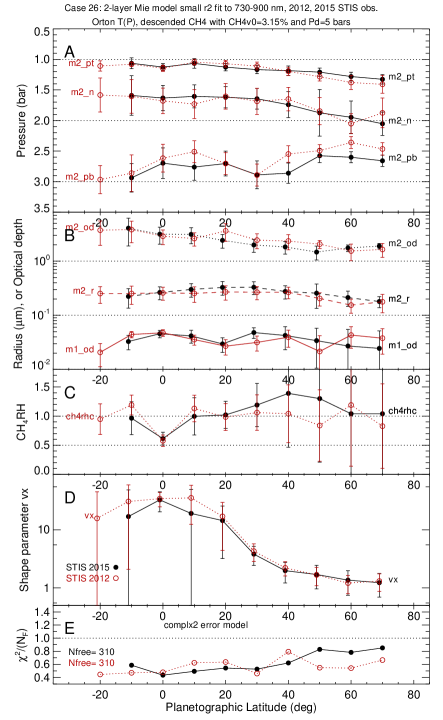
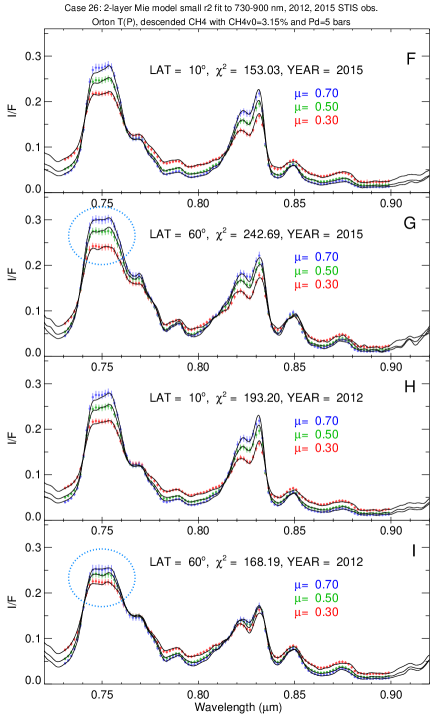
Figure 25.— Descended depletion model of vertical methane distribution fit to STIS spectra from 2012 and 2015. Conservative cloud model and gas profile parameters for a Mie-scattering haze above a single diffuse Mie-scattering tropospheric layer, assuming a deep mixing ratio of 0.0315, and a methane profile characterized by a pressure depth parameter $P_{d}$ and a shape parameter $vx$ (defined in Eq. 8.3 and illustrated in Fig. 14) and constrained by spectral observations from 730 nm to 900 nm. The parameter values are in panels A-E, with red (open circle) points displaying results of fitting 2012 STIS observations and black (filled circle) points displaying the results of fitting 2015 observations. Sample comparisons between measured and large-particle model spectra are in panels F-I. Note the great improvement in the high latitude fits near 745 nm, compared to results given in Fig. 20.

Table 13Two-cloud spherical particle fits as a function of latitude assuming descended depletion of CH₄ as a function of latitude.

Lat.	$m1\_od$		$m2\_pt$	$m2\_pb$	$m2\_r$
(∘)	$\times$100	$m2\_od$	(bar)	(bar)	($\mu$m )	$m2\_nr$	$ch4rhc$	$vx$	$\chi^{2}$	YR
-10	3.3$\pm$1.0	4.06$\pm$2.15	1.06$\pm$0.09	2.94$\pm$0.23	0.22$\pm$0.09	1.59$\pm$0.32	0.96$\pm$0.28	16.90$\pm$31.60	181.84	2015
0	4.6$\pm$0.7	3.14$\pm$1.09	1.13$\pm$0.06	2.70$\pm$0.25	0.26$\pm$0.07	1.63$\pm$0.21	0.61$\pm$0.11	32.70$\pm$12.30	134.79	2015
10	4.2$\pm$1.1	3.12$\pm$1.02	1.07$\pm$0.08	2.76$\pm$0.22	0.30$\pm$0.08	1.61$\pm$0.19	1.00$\pm$0.32	19.10$\pm$30.30	153.03	2015
20	3.0$\pm$0.9	2.42$\pm$0.69	1.13$\pm$0.06	2.70$\pm$0.20	0.33$\pm$0.09	1.62$\pm$0.17	1.02$\pm$0.23	14.40$\pm$11.20	168.49	2015
30	4.8$\pm$1.1	1.99$\pm$0.54	1.17$\pm$0.07	2.89$\pm$0.23	0.33$\pm$0.09	1.64$\pm$0.17	1.19$\pm$0.37	3.81$\pm$ 1.38	163.38	2015
40	4.2$\pm$1.9	1.83$\pm$0.48	1.18$\pm$0.08	2.86$\pm$0.17	0.28$\pm$0.08	1.74$\pm$0.21	1.39$\pm$0.93	1.98$\pm$ 0.76	192.65	2015
50	3.4$\pm$2.4	1.47$\pm$0.42	1.21$\pm$0.07	2.58$\pm$0.11	0.26$\pm$0.12	1.87$\pm$0.38	1.30$\pm$1.09	1.70$\pm$ 0.74	256.78	2015
60	2.7$\pm$2.8	1.75$\pm$0.24	1.28$\pm$0.07	2.60$\pm$0.09	0.21$\pm$0.07	1.95$\pm$0.27	1.04$\pm$1.14	1.36$\pm$ 0.61	242.69	2015
70	2.5$\pm$2.7	1.90$\pm$0.22	1.33$\pm$0.08	2.66$\pm$0.09	0.18$\pm$0.04	2.05$\pm$0.19	1.04$\pm$1.18	1.23$\pm$ 0.54	263.79	2015
-20	2.1$\pm$0.9	3.73$\pm$1.77	1.11$\pm$0.08	2.97$\pm$0.23	0.25$\pm$0.09	1.58$\pm$0.28	0.95$\pm$0.26	15.70$\pm$29.40	138.18	2012
-10	4.4$\pm$0.6	3.82$\pm$1.64	1.08$\pm$0.03	2.86$\pm$0.30	0.25$\pm$0.09	1.61$\pm$0.28	1.19$\pm$0.17	30.70$\pm$28.60	145.93	2012
0	4.8$\pm$0.7	2.89$\pm$0.87	1.15$\pm$0.05	2.62$\pm$0.23	0.26$\pm$0.07	1.68$\pm$0.21	0.58$\pm$0.10	34.30$\pm$ 9.49	148.60	2012
10	3.6$\pm$0.7	2.61$\pm$0.71	1.04$\pm$0.05	2.51$\pm$0.18	0.25$\pm$0.08	1.73$\pm$0.24	1.13$\pm$0.23	35.40$\pm$23.00	193.20	2012
20	2.7$\pm$0.9	3.62$\pm$1.30	1.07$\pm$0.06	2.70$\pm$0.18	0.27$\pm$0.08	1.60$\pm$0.21	0.98$\pm$0.23	17.00$\pm$12.60	197.04	2012
30	3.2$\pm$1.0	2.44$\pm$0.75	1.11$\pm$0.06	2.89$\pm$0.18	0.27$\pm$0.07	1.69$\pm$0.21	1.06$\pm$0.31	4.29$\pm$ 1.45	142.42	2012
40	3.9$\pm$1.4	2.35$\pm$0.74	1.20$\pm$0.07	2.55$\pm$0.13	0.27$\pm$0.06	1.65$\pm$0.19	1.04$\pm$0.50	2.21$\pm$ 0.61	245.82	2012
50	2.2$\pm$2.1	2.06$\pm$0.35	1.28$\pm$0.07	2.49$\pm$0.10	0.20$\pm$0.06	1.85$\pm$0.22	0.84$\pm$0.61	1.67$\pm$ 0.58	170.15	2012
60	4.3$\pm$1.9	1.54$\pm$0.52	1.38$\pm$0.11	2.36$\pm$0.10	0.15$\pm$0.04	2.05$\pm$0.16	1.19$\pm$1.05	1.21$\pm$ 0.41	168.19	2012
70	3.8$\pm$1.9	1.65$\pm$0.47	1.41$\pm$0.15	2.47$\pm$0.10	0.18$\pm$0.07	1.88$\pm$0.24	0.83$\pm$0.73	1.31$\pm$ 0.44	206.35	2012

NOTE: The optical depth is for a wavelength of 0.5 $\mu$m. These fits used a fixed value of $Pd=$ 5 bars, $\alpha_{0}=$ 3.15%. There were 318 points of comparison and 8 fitted parameters, for a nominal value of NF=310, for which the normalized $\chi^{2}$ /NF ranged from 0.42 to 0.83.

These two depletion model fits are compared in Fig. 26, with descended model fits in panel A and the stepped depletion model fits in panel B. The descended model fits yield slightly lower $\chi^{2}$ values, especially at 70^∘ N, although even there the difference is smaller than the expected uncertainty of $\sqrt{2\chi^{2}}$, which is 22 in this case. Both models imply that the high latitude depletion is of limited depth, and both imply that the methane humidity above the 1 bar level is near saturation at low latitudes and decreases poleward. Not only can we obtain good fits with a shallow depletion of methane, they are preferred on the basis of fit quality. Not only does the high latitude fit near 745 nm improve significantly when the vertically varying depletion models are used, but the overall $\chi^{2}$ at high latitudes is also significantly improved, as illustrated in Fig. 27. This is especially apparent at the higher latitudes and in comparing averages over the 50^∘ – 70^∘ latitude range. Although the stepped depletion model is seen to yield slightly better $\chi^{2}$ values than the descended depletion models, the difference is less than the expected uncertainty. The virtue of the stepped depletion model is that it can be well constrained at all latitudes, while the virtue of the descended depletion model is that it makes more sense physically. We were able to extend the latitude range of the descended model fits by fixing the value of the depth parameter $P_{d}$ to 5.0 bars. We then found that both depletion models do not quite yield zero depletion at low latitudes, which one might interpret to mean that we should have chosen a slightly lower deep methane VMR value. However, the $\chi^{2}$ values for the vertically uniform values are just as good or slightly better than the depleted models at low latitudes.

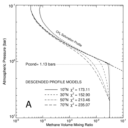
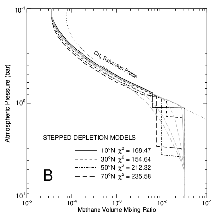
Figure 26.— A: Best-fit descended profiles at 4 latitudes, using average parameter fits for 2012 and 2015. B: Best fit stepped depletion profiles, using average parameter fits for 2012 and 2015. The profiles in A are overlain in light gray in B for reference. Both sets of fits show decreasing methane humidity with latitude above the 1 bar level, and both indicate that the depletion is of limited depth ($\sim$5 bars or less). In both cases average $\chi^{2}$ values for 2012 and 2015 are given in the legend.

Figure 27.— Comparison of 2012 (left) and 2015 (right) $\chi^{2}$ versus latitude values for for three different methane vertical distribution models: uniform (solid line), descended depletion (dotted line), and stepped depletion (dashed line). Corresponding averages over the 50^∘ – 70^∘ latitude range are also shown near 80^∘N in each panel. The depleted profile values are slightly shifted in latitude to avoid error bar overlaps. This shows that the overall fit quality is improved by use of the descended profile, in addition to the more obvious improvement near 750 nm. The small overall improvement seen in fits to the 2015 observations is likely due to the increased noise level at high latitudes and low signal levels for this data set.

9.4. Wavelength dependence issues

Although the best-fit parameters given in Table 7 provide great spectral matches over the fitted range (730–900 nm), they do not provide good matches over the entire range. As expected, and as illustrated in Fig. 28, the corresponding model spectra fit even worse over the rest of the wavelength range than the initial fit shown in Fig. 16. The problem with both the small-particle and large-particle models is that they do not produce a large enough I/F at the short wavelength side of the spectrum (from 0.54 $\mu$m to 0.68 $\mu$m) for the two largest zenith angle cosines, and produce too high an I/F in the deeply penetrating region near 0.94 $\mu$m for all three zenith angles. The problem is less extreme for the small-particle solution because it produces a larger increase in I/F at shorter wavelengths.

One way to solve the short wavelength deficit problem is to abandon spherical particles and use a wavelength-dependent phase function that provides increased backscatter at short wavelengths, which is the approach followed by KT2009, and one which we will return to in a later section. An alternative approach considered here is to use a wavelength-dependent imaginary index that is small at short wavelengths and larger at long wavelengths, an approach used by Irwin et al. (2015) to solve a similar problem in fitting near-IR spectra. The utility of this approach is that the increased optical depth required to compensate for the small absorption at long wavelengths leads to a needed increase in the I/F at short wavelengths where the absorption is absent. To follow up on this approach we added an adjustable imaginary index to cloud particles in the m2 Mie layer, and then optimized model parameters to fit both the 730–900 nm region and the 540-580 nm region simultaneously, as described in the following section.

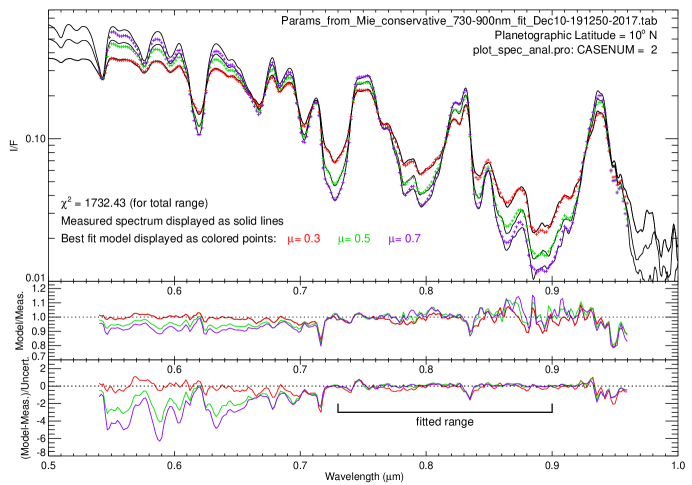
Figure 28.— As in Fig. 16, except 10^∘ N spectral comparisons are shown for a conservative cloud model that provide the best match to the 10^∘ N 2015 STIS spectra from 730 nm to 850 nm, using the small particle solution. Note the significant model falloff at shorter wavelengths. See text for implications.

9.4.1 Controlling wavelength dependence with particulate absorption

The first example of controlling wavelength dependence over a larger spectral range is based on adjustment of particulate absorption. For this example, we assume two Mie scattering clouds, with the top layer (m1) located at an arbitrary pressure of 50 mbar and containing conservative particles with an assumed effective radius of 0.06 $\mu$m, and an adjustable optical depth. The top layer has a very small optical depth and its particle size is not very well constrained by our observations. We chose a somewhat arbitrarily value based on preliminary fitted values. The Rages et al. (1991) haze model estimates a particle size closer to 0.1 $\mu$m at 50 mbar. The other Mie layer is assumed to be composed of a non-conservative material, characterized by a refractive index of $m2\_nr$ + 0 $\times$ $i$ for $\lambda<$700 nm and n = $m2\_nr$ + $m2\_ni\times i$ for $\lambda>$ 710 nm. The tropospheric Mie layers (m2) is characterized by three additional fitted parameters: pressure, particle size, and optical depth. We then simultaneously fit just two sub regions of the spectrum: the 540-580 nm region, where we assume the particles are conservative, and the 730–900 nm region, where we assume a locally wavelength-independent imaginary index that is adjusted to minimize $\chi^{2}$. We also allowed $m2\_nr$ to be adjustable. This process produced a best-fit value of (4.9$\pm$1.3)$\times 10^{-3}$ for the imaginary index and 2.7$\pm$0.3% for the deep methane mixing ratio. However, this process slightly degraded the fit in the 730-900 nm region. To better constrain the methane mixing ratio for the case with absorbing aerosols we adopted the imaginary index obtained from the dual fit, then refit the remaining parameters using the 730-900 nm region for our spectral constraints, yielding the results given in Table 10. Applying these parameters over the entire spectral range from 540 nm to 960 nm, we then obtained a much improved match to the observations, with a $\chi^{2}$ of 724.50. This was further improved to 586.32 by optimizing values of $m2\_pt$ (1.09$\pm$0.01 bar), $m2\_pb$ (3.35$\pm$0.13 bar), $m1\_od$ (0.030$\pm$0.002), $m2\_od$ (3.91$\pm$0.34), $m2\_r$ (0.30$\pm$0.02), $m2\_nr$ (1.69$\pm$0.04), and $m2\_nilw$ (0.0051$\pm$0.0003), after adding an intermediate imaginary index of 0.0011 to the tropospheric aerosol particles in the spectral interval from 670 nm to 730 nm, yielding the fit displayed in Fig. 29. Although the fit is good, it is not known whether any plausible cloud material has this absorption characteristic. Complex hydrocarbons, such as tholins (Khare et al., 1993), absorb more at shorter wavelength and have declining absorption over the range where our example model shows increased absorption. Judging from frost reflection spectra obtained by Lebofsky and Fegley (1976), H₂S does not appear to exhibit such a trend either. Thus we have some motivation to consider other ways to generate wavelength dependence.

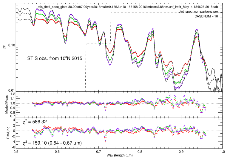
Figure 29.— Extended range wavelength dependent model, using imaginary index variations to adjust the wavelength dependence. The imaginary index $m2\_ni$, multiplied by a factor of 100, is shown by the dashed curve.

9.4.2 Controlling $\lambda$ dependence with optical depth variations

Although Mie scattering calculations for spherical particles produce wavelength dependent optical depth and scattering phase functions, if these do not yield needed dependencies, and if particle size is constrained, and wavelength-dependent absorption is not acceptable, then non-spherical particles need to be considered.

The simplest option is to use a single HG scattering phase function and simply adjust the wavelength dependence of the optical depth to match the observed spectral variation. An increase in optical depth with size parameter (2$\pi r/\lambda$) is certainly a characteristic shared by most particles and by aggregates in our trial calculations. It also is plausible that a non-spherical particle might exhibit a greater $\lambda$ dependence in optical depth than a spherical particle for the case in which both particles satisfy the other constraints in the 730-900 nm region. To define the needed $\tau(\lambda)$ function we began by taking our best fit vertical structure and asymmetry fit for the 730-900 nm region, then computed a series of model spectra with optical depths increasing until we could find an optical depth at any wavelength that would match the observed I/F at that wavelength. But we found a problem with this approach. At short wavelengths, the optical depth needed to match two successive continuum regions (e.g. at 560 nm and 585 nm) was about 4-5 times the value at 800 nm that was derived from fits to the 730-900 nm region. But to match the intervening absorption feature at 576 nm would require about half of that optical depth. Thus a smoothly varying optical depth function could not be created in this fashion, and a function that included wiggles at all the methane features was completely implausible. The fix to this problem was to distribute the cloud particles over a greater atmospheric depth. This would not change the continuum I/F values very much, but in the weakly absorbing regions, there would be more absorption. At longer wavelengths this required an increase in the cloud’s optical depth, which in turn required readjustment of the optical depth ratio between 800 nm and 540 nm. The result of this process applied to our model of the 2015 STIS spectrum at 10^∘N is shown in Fig. 30.

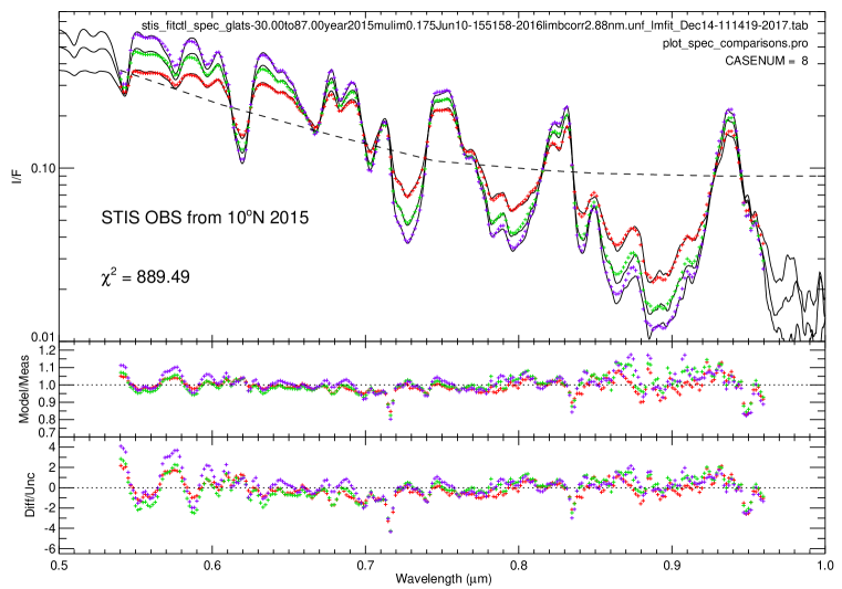
Figure 30.— Extended range wavelength dependent model for HG particles, using an optical depth variation with wavelength adjusted to match the 2015 STIS observations at 10^∘N. The dashed curve displays the wavelength dependent optical depth normalized by its value at 800 nm, then scaled downward by a factor of 10.

9.4.3 Controlling $\lambda$ dependence with phase function variations

KT2009 assumed that the main tropospheric cloud layer had a wavelength-independent optical depth, which is a plausible assumption for large particles, and used a wavelength dependent phase function to match the observed spectral variation. A general form of their function can be written as

$$f_{1}(\lambda)=a-b\times\sin^{\alpha}[\frac{\pi}{2}(\lambda_{o}-\lambda)/(\lambda_{0}-\lambda_{1})],$$ (6)

$$\lambda_{1}\leq\lambda\leq\lambda_{o}$$

in which KT2009 assumed $\alpha=4$, $a=0.94$, $b=0.427$, $\lambda_{0}=1$ $\mu$m, and $\lambda_{1}=0.3$ $\mu$m, which makes $f_{1}$ reach a maximum of 0.94 at a wavelength of 1 $\mu$m and a minimum of 0.513 at 0.3 $\mu$m. They applied this to a double HG function with adopted values of $g_{1}$ = 0.7 and $g_{2}$ = -0.3. (Note that there is no basis for applying this function to wavelengths greater than 1 $\mu$m or less than 0.3 $\mu$m.) We found that this function was able to fit low latitude spectra over the 730 nm to 900 nm range quite well, but that the $a$ and $b$ constants needed to vary with latitude and that we needed to increase $g_{1}$, leading us to adopt a new value of 0.8. When applied to the extended spectral range, we needed to increase $\lambda_{1}$ to about 0.45 and $\alpha$ to 5. The resulting spectral match was intermediate between those shown in Figs. 29 and 30. A problem with this formulation is that extending the idea to longer wavelengths would require the particles to become more and more forward scattering at longer wavelengths (in order to produce the same effect that absorbing Mie particles produce, as discussed later). This is not a plausible trend. For large enough wavelengths the particles must become less forward scattering.

We also considered whether the HG model could use a wavelength-dependent asymmetry parameter instead of a wavelength dependent optical depth to match the observed spectrum over a wider spectral range. However, matching the shorter wavelengths required a negative asymmetry parameter, which is an implausible condition, and thus not an acceptable solution.

Thus over the longer spectral ranges it is most likely that optical depth variation and possible particulate absorption will be needed to model reflected spectra. Phase function variations will also be present, but cannot be the sole way to produce the needed wavelength dependence in scattering properties.

9.5. Two-layer Mie model applied to Near-IR spectra

To test whether our 2-layer Mie models would be capable of fitting near-IR spectra, we extended model calculations to 1.6 $\mu$m and compared them to a central meridian SpeX spectrum covering the 0.8–1.65 $\mu$m range. [We obtained this spectrum from the Infrared Telescope Facility on 18 August 2013, using the cross-dispersed mode of the SpeX spectrometer. The spectrum was spatially averaged over the central 0.4 arcseconds of the central meridian covered by the 0.15-arcsecond slit, corresponding to an average latitude of 24^∘N. It was spectrally smoothed to the same spectral resolution as the smoothed STIS spectrum (a FWHM of 2.88 nm). The spectrum was scaled to match the 1.09$\times 10^{-2}$ I/F center-of-disk H-band I/F from Sromovsky and Fry (2007).] The initial small-particle model parameters we used were from the 20^∘N spectrum and used an imaginary index of 0.0046 at all wavelengths longer than 730 nm. For the initial large-particle model, we used a fit to the 10^∘N spectrum and used an imaginary index of 6.2$\times 10^{-4}$ for $\lambda>$ 730 nm. The smaller index for the large particle solution is a result of the lower real refractive index for the best-fit larger particles.

Fig. 31 shows that the extended models agree well in the dark regions of the spectrum, indicating that little change in stratospheric haze properties is needed, but is far too bright in the longer wavelength continuum regions, indicating that the real cloud particles have, at longer wavelengths, a lower optical depth or greater absorption than the model particles. The large particle solution is the worst offender because its scattering efficiency is a relatively weak function of wavelength, while the scattering efficiency of the smaller particles declines substantially, though not enough to match the falloff in pseudo continuum I/F values with wavelength.

The excess model I/F at these wavelengths can be reduced by increasing the imaginary index as indicated in the bottom panel of Fig. 31. Our procedure for developing these solutions was to start with a conservative solution constrained by the 730-900 nm spectrum. We then used that as an initial guess for a split fit of the 540-580 nm plus 730-900 nm region, assuming that the imaginary index was zero for $\lambda\leq$ 580 nm and had an adjustable value of $m2\_nilw$ for for $\lambda\geq$ 730 nm. From that we obtained an estimate for the imaginary index in the 730-900 nm region. We then fixed that imaginary index and did a new fit within the 730-900 nm region to get a revised estimate of the methane profile. We then fixed the methane profile and used a second split fit to improve the optical depth and vertical aerosol distributions, as well as particle size and real index. We then adjusted the imaginary index in the 670-730 nm range to optimize the fit to that part of the spectrum. That provided the parameters used for the initial near-IR calculations. To match the near-IR spectrum we did a suite of forward calculations with different constant imaginary index values to find in each wavelength region the imaginary index that provided the best model match to the observations. This was not done at a fine wavelength resolution in an attempt to match every detail because the solid materials making up the cloud particles would not likely have such fine-scale absorption features.

This figure shows that the STIS-based model with two layers of small spherical particles can match the observed infrared spectrum out to 1.65 $\mu$m by increasing the imaginary index with wavelength as shown in Fig. 31, reaching a maximum of 0.1 for the H-band region. Our index is generally larger than the imaginary index estimated by Irwin et al. (2015) although of roughly similar shape. Our mean value in the H band is similar to the adopted value of de Kleer et al. (2015). Our fitted real index of 1.72$\pm$0.2 for the extended-wavelength small-particle model is significantly larger than the value of 1.4 assumed by Irwin et al. (2015). Since our particles are thus inherently brighter, it is not surprising that we might need more absorption than Irwin et al. to match the observations. Our large-particle model, with a lower real index, has an imaginary index profile of similar shape but lower amplitude. The imaginary index value for de Kleer et al. (2015) we derived from their assumed single-scattering albedo of 0.75, which corresponds to an imaginary index of 0.06 for 1-$\mu$m particles. Irwin et al. suggested that the refractive index spectrum would allow us to determine the composition of the cloud particles. However, the most likely cloud material (H₂S) does not have well characterized (quantitative) absorption properties, and frost reflection spectra between 1.2 and 1.6 $\mu$m (Fink and Sill, 1982) provide little qualitative evidence for significant absorption of the type we seem to need to match the observed spectrum.

We could also have modeled the drop in I/F at longer wavelengths using a HG particle scattering model, either by varying the single-scattering albedo with wavelength, or by varying the optical depth as a function of wavelength. It is left for future work to evaluate which sort of variation provides the best overall compatibility with the observations.

Although our modified imaginary index allows our two cloud model to closely reproduce the observed spectrum in most regions, there are some problems that need further work to address. First, note that at the 1.08-$\mu$m continuum peak, the model contains modulations that are not observed in the measured spectrum. This is also the case for model calculations shown by Tice et al. (2013), and is an indication of a possible flaw in our commonly used absorption coefficients in this region.

There is also a relatively sharp feature at 1.1 $\mu$m that is much larger in the model than in the observations. Further, the detailed shape of the pseudo continuum peak near 1.27 $\mu$m is not fit very well.

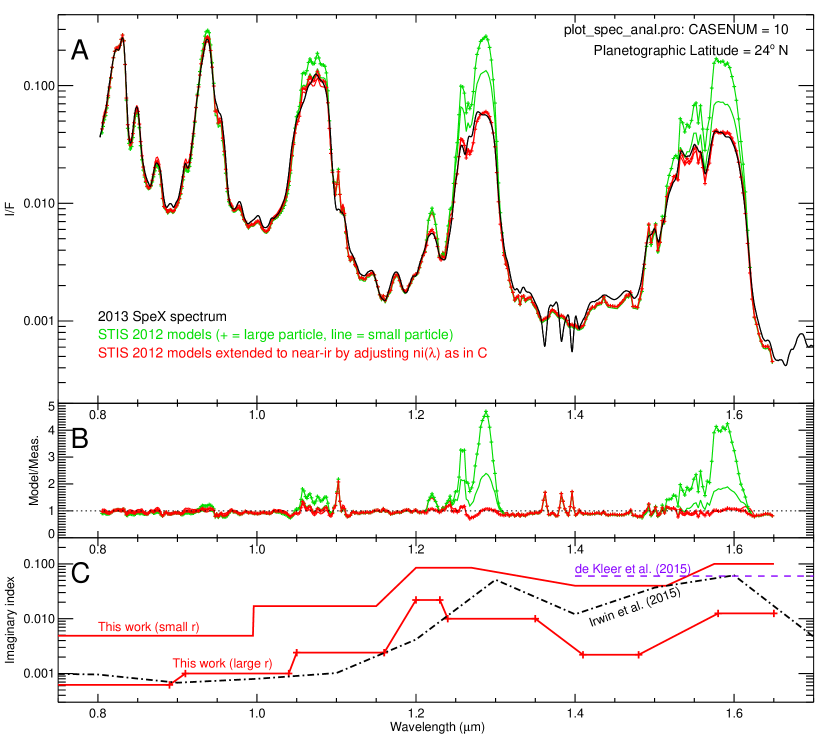
Figure 31.— A: Our 2013 SpeX near-IR spectrum of Uranus from latitude 24^∘ N (black) compared to model spectra for the same observing geometry but using the gas and aerosol parameters from the 20^∘ N two-layer Mie scattering model for two particle size solutions: small-particle (line only) and large-particle (lines with points). The same models, extended to the near-IR by adjusting the imaginary index of the cloud particles, are shown in red. In the first model set of models, a vertically uniform methane mixing ratio of 2.65% was assumed up to the methane condensation level. In the second set (red curves) a deep mixing ratio of 3.15% was assumed and a descended depletion profile shape was used, with vx = 7.34 an Pd = 5 bars. B: ratio of model spectra to the SpeX observed spectrum. C: Imaginary index spectra assumed in the second set of models (red), compared to imaginary index values derived by Irwin et al. (2015) and a value inferred from a single scattering albedo used by de Kleer et al. (2015).

10. Discussion

10.1. Why occultation constrained fits produced larger methane VMR values

Given the previous discussion of methane depletion profiles, this might be a good point at which to compare the methane profiles in Fig. 26 with those obtained from the occultation analysis of Lindal et al. (1987) or Sromovsky et al. (2014). This is provided in Fig. 32, where we also show the results of Orton et al. (2014b) and Lellouch et al. (2015). The main regions of sensitivity to the methane VMR values are indicated by thicker lines for our current STIS results and those of Lellouch et al. (2015). Note that our current STIS results at 30^∘ N are in very good agreement with the Lellouch et al. results where they have overlapping sensitivity (roughly the 200–700 mbar range). Both have relatively high methane relative humidities compared to the saturation vapor pressure profile computed for the Orton et al. (2014a) thermal profile. The occultation results for methane are at much lower levels at pressures less than the putative methane condensation pressure (about 1.2 bars). In the occultation analysis, temperature and methane profiles are linked. Both temperature and composition affect density, which in turn affect refractivity versus altitude, which is the main result produced from the radio measurements. The refractivity profile can be matched by a family of thermal and corresponding methane profiles. A hotter atmosphere is less dense, and thus allows more methane to produce the same refractivity. Because the occultation profiles have such low relative methane humidities above the cloud level compared to what the STIS spectra require to obtain the best fits, the hottest occultation profile is favored. If the only allowed adjustment of methane is selection of the optimum occultation profile, as was the case for our previous analyses (Sromovsky et al., 2011, 2014), then we obtain a deep mixing ratio that is relatively high (4%) so that the methane mixing ratio near and above the cloud level can approach closer to the level needed to provide the best spectral match. As an example of this behavior, we carried out fits of STIS spectra at 10^∘ N, using STIS spectral fit quality as the only constraint, and compared that to the best fits obtained for profiles with fixed occultation consistent methane vertical profiles. The results, tabulated in the legend of Fig. 32, show that all the occultation fits are much worse than the STIS-only constrained fits, and that the best of the occultation constrained fits (for the F profile) is for the hottest profile, which provides the most upper tropospheric methane, even though that has a deep methane VMR that is much higher than is needed if one does not force the methane to fit an occultation profile. Just below the cloud level, the methane VMR at low latitudes is closer to 2% at least in the region above the lower tropospheric clouds (near 2.5 bars) and perhaps deeper, although the STIS spectra are not sensitive to values deeper than that.

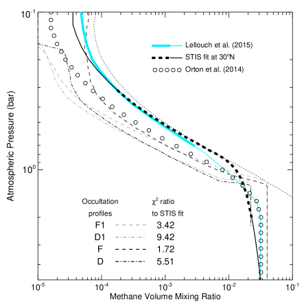
Figure 32.— Comparison of methane profiles derived from STIS-constrained and other spectral observations by Lellouch et al. (2015) and Orton et al. (2014b) compared to those derived from occultation observations by Lindal et al. (1987) and Sromovsky et al. (2011). The 4% deep methane VMR occultation profiles provide better agreement with STIS-constrained results in the upper troposphere. But without occultation constraints, the preferred deep mixing ratio is closer to 3% for most aerosol models fit to the 730-900 nm spectrum.

10.2. Evidence for a deep cloud layer

In our previous paper dealing with earlier STIS observations (Sromovsky et al., 2014), we found that the fit quality at short wavelengths was improved by adding a deep cloud layer, which we fixed at the 5 bar level and assumed had the same tropospheric scattering parameters as KT2009. The only adjustable parameter for that layer was its wavelength-independent optical depth, which we found to vary from about 4 at low latitudes to about half that at high latitudes. It is possible in our current modeling that the more extended vertical extent of our upper tropospheric cloud layer serves to reduce the need for the contribution of a deeper cloud. The main function of the deeper cloud is to improve the fit in the 540 to 600 nm range where matching weak methane band depth is easier if some of the aerosol scattering is moved to higher pressures.

To provide a better test of the existence of a deeper cloud, we looked at spectra with deeper penetration. Choosing a spectrum with a nearly vertical view ($\mu$ = 0.9 at 10^∘N), we computed simultaneous model spectra for view angle cosines of $\mu$ = 0.3, 0.5, and 0.9, based on the fit we obtained using the standard set of view angle cosines ($\mu$ = 0.3, 0.5, and 0.7). That model did not fit the weak methane bands very well even with the standard view angles and was even worse for this more deeply penetrating set. The $\chi^{2}$ values rose from 586.32 to 714.59, with an expected $\chi^{2}$ uncertainty of 35-40. This $\chi^{2}$ increase by 128.3 is about three times its uncertainty. However, by refitting the same model (still without a deep cloud) to the new set of view angles, we reduced the $\chi^{2}$ value for this new set of angles to 705.84, and thus reducing the difference to 119.5, which is still about three times the expected uncertainty in $\chi^{2}$. After inserting an optically thick deep cloud with an adjustable pressure, a new fit further reduced $\chi^{2}$ from 705.84 to 645.62, a decrease of 59.52, which is about 1.6 times its uncertainty. A comparison of the latter and initial fits to the measured spectra is displayed in Fig. 33. The $\chi^{2}$ improvement is even more dramatic when computed just for the region from 540 nm through 670 nm. In that case the $\chi^{2}$ change is from 180.53 to 125.17, a decrease of 75.46, which is over three times the expected uncertainty of about 22 for this more limited range that has 243 comparison points. The model with a deep cloud also improved fits at the original set of view (and zenith) angles. Adding that layer to the model plotted in Fig. 29 and refitting, decreased $\chi^{2}$ from 586.32 to 529.95, a decrease of 56.37, with most of this change taking place in the 540-670 nm region where $\chi^{2}$ dropped from 159.10 to 102.47, a decrease by 56.63, which is about 2.6 times the expected uncertainty. Thus both sets of view angles lead to significant local fit improvements, with derived effective pressures of 10.6$\pm$0.4 bars for the more deeply penetrating view angles and 9.5$\pm$0.5 bars for our standard set. A better estimate for the effective pressure of an optically thick deep cloud is probably 10$\pm$0.5 bars. A lower pressure is likely if the cloud is not optically thick. When we fixed the deep cloud pressure at 5 bars the best-fit optical depth of the cloud was 4.2$\pm$0.7 (using the more deeply penetrating spectral constraints). This is quite consistent with the optical depth of the 5-bar deep cloud fits of Sromovsky et al. (2014). Further investigation of the nature of this deep cloud layer, including its latitude dependence, is left for future work. A plausible composition for such a cloud is NH₄SH.

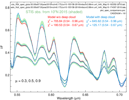
Figure 33.— STIS 2015 observations at 10^∘N (green shading indicating uncertainties), compared to fitted model results without a deep cloud layer (red) and with a deep cloud layer (blue). These are for non-standard, more deeply penetrating, zenith angle cosines of 0.3, 0.5, and 0.7, with largest cosines corresponding to largest I/F values at continuum wavelengths. The legend gives $\chi^{2}$ values for the entire spectral range that was fitted (0.54 - 0.96 $\mu$m) and for the region most influenced by the deep cloud (0.54 - 0.70 $\mu$m).

10.3. Comparison with other models of gas and aerosol structure on Uranus.

Models of 0.8-1.8 $\mu$m SpeX spectra of Uranus by Tice et al. (2013) and more recently by Irwin et al. (2015) and recent models of H-band (1.47-1.8 $\mu$m) spectra by de Kleer et al. (2015) present what appear to be different views of the cloud structure from that derived from our STIS observations. Some fraction of the differences are due to different constraining assumptions. The other authors typically constrain the upper cloud boundary pressure and fit the scale height ratio, while we have here mainly assumed a unit scale height ratio (particles uniformly mixed with gas) and treated the upper boundary pressure as adjustable. The differences are probably not due to very different conditions on Uranus, as the spectral observations are generally very similar, as illustrated in Fig. 34. These spectra are all obtained near the center of the disk, and all near latitude 20^∘ N. In most of the spectral range they are all within 10% of each other. The main exception is the de Kleer et al. (2015) spectrum, which is much brighter than the other two spectra in the 1.63-1.8 $\mu$m region. This would presumably lead to a model with much greater stratospheric haze contributions than would be needed to match the other spectra. To better characterize these differences and better understand their origin, we attempted to reproduce results from these near-IR analyses.

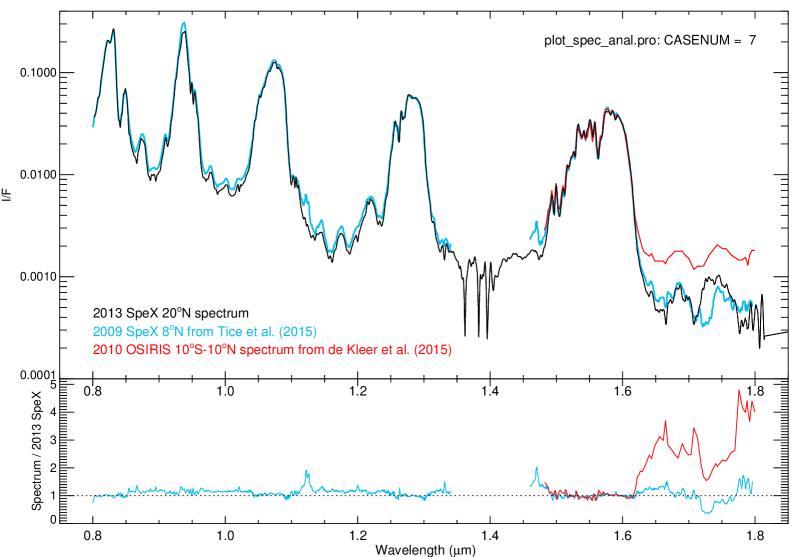
Figure 34.— Comparison of near-IR spectra of Uranus. Our 2013 central-disk spectrum is shown in black. The 2009 SpeX central-disk spectrum of Tice et al. (2013) is shown in blue, and the 2010 OSIRIS 10^∘S - 10^∘ N spectrum of de Kleer et al. (2015) in red. The bottom panel plots the ratio of each spectrum to our 2013 SpeX spectrum.

The first attempt was to match the Irwin et al. (2015) retrieval of a two-cloud structure from the Tice et al. (2013) 2009 SpeX central meridian data (0.8-1.8 $\mu$m range). They used 1.6% deep CH₄ with 30% RH above condensation level and the Lindal et al. (1987) Model D T(P) profile. They retrieved self-consistent refractive indexes for their Tropospheric Cloud (TC) and Tropospheric Haze (TH), similar to Tice et al. 2-cloud model. They retrieved particle sizes, but used ”combined H-G” phase function fits in the forward modeling, rather than Mie calculations. An additional complication was that their plots of optical depth vs pressure were incorrect in the paper (estimated to be about an order of magnitude too large, P.G.J. Irwin private communication). That and the uncertain way double HG phase functions were obtained from the Mie phase functions, led us to not attempt detailed quantitative comparisons.

We decided to make our quantitative comparisons with 2-cloud results of Tice et al. (2013). This was more tractable, as the phase functions for both TC (tropospheric cloud) and UH (Upper Haze, called TH in Irwin et al.) were simply H-G phase functions with an assumed asymmetry parameter g = 0.7. They also utilized wavelength-dependent optical depths based on Mie calculations of extinction efficiency, but they did not use the wavelength-dependent phase functions or wavelength-dependent asymmetry parameters for either particle mode. Although, for the larger particles in the TC, the asymmetry parameter obtained from Mie calculations is close to their chosen value, the 0.1-$\mu$m particle model has a very small asymmetry, which leads to a backscatter phase function value about ten times that for an HG function with g = 0.7. Since their UH (or TH) particles have such small optical depths, their contribution can be well approximated by single-scattering, in which case the observed I/F contribution is given by

$$I/F=\frac{1}{4}\varpi P(\theta)\tau/\mu$$ (7)

where $\theta$ is the scattering angle (about 180^∘ in this case), $\tau$ is the vertical optical depth, and $\mu$ is the cosine of the observer zenith angle. This makes the modeled I/F strongly dependent on the assumed phase function, specifically its backscatter amplitude. While there is substantial variation in scattering efficiency with wavelength for a 0.1-$\mu$m particle, such a particle would not have such a strongly forward peaked phase function, and would probably require roughly a factor of ten lower optical depth than Tice et al. (2013) found for their UH layer. However, using their peculiar scattering characterization for this layer, and using their more plausible characterization for the lower layer, and their chosen single-scattering albedos, we were able to roughly match our own 2013 SpeX center-of-disk spectra (which are quite similar to the spectra shown in the Tice paper). Thus we have two different vertical structures that can match the spectra. Ours has a single tropospheric layer uniformly mixed between 1.06 and 3.3 bars (small particle solution), while theirs has a very strongly varying optical depth per bar between their assumed cloud top of 1 bar and their fitted bottom at 2.3 bars. We did not attempt to reproduce the more complex structures based on Sromovsky et al. (2011) three- and four-cloud models.

We also tried to reproduce de Kleer et al. (2015) results for a 2-cloud model. Their retrievals were for a more limited H-band wavelength range (H-band spectra). Their spectra were also similar to our 2013 SpeX results, except their dark regions were as much as 3-4 times brighter (see Fig. 34). They used a two-stream radiative transfer model, with wavelength dependent H-G parameters based on Mie calculations. Using their retrieved optical depths, we roughly matched their window I/F. However, we used correlated-k coefficients for Hartmann type line-shape wings, while de Kleer et al. used the hybrid wing shape from Sromovsky et al. (2012a) that produces more absorption in the H-band window. Using these c-k coefficients, our I/F values in the methane window were lower than those of de Kleer et al. by a factor of 2 or so. The origin of these differences remain to be determined. It is likely that it is not entirely a result of very different numbers of streams, as de Kleer et al. did trial calculations showing that their approximation was good to within $\sim$10%.

A comparison of the characteristics of the tropospheric cloud models from aforementioned references is displayed in Fig. 35. Although all of these models provide good fits to the spectra (ignoring the fact that we could not reproduce all these results), they have very different vertical structures and total optical depths and column masses. In fact the widest variation in total cloud mass is between our own small-particle and large-particle solutions. In the log-log plot in Fig. 35A, the various cloud structures seem more similar than in the linear plot in panel B, where the huge differences in optical depths and mass loading are more accurately conveyed. The column number density in particles per unit area is computed as $n=\tau/(\pi r^{2}Q_{ext}$), where $r$ is the particle radius and $Q_{ext}$ is the extinction efficiency (extinction cross section divided by geometric cross section). From $n$ the mass loading (mass per unit area) is computed as $m$ = $n\rho\pi r^{3}$, assuming that the particle density $\rho$ is 1 g/cm³. Our small-particle tropospheric cloud is one of very low maintenance. It needs very little material to form, the particles fall slowly because they are small, and thus probably a low level of mixing is needed to sustain it. It also has the virtue of having a refractive index similar to that of its potential main component, H₂S. The large particle cloud is thirty times more massive, with larger particles that fall much more quickly, needing much more vertical transport to be sustained.

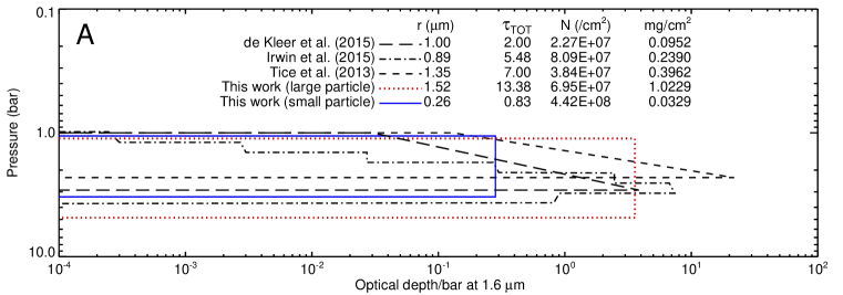
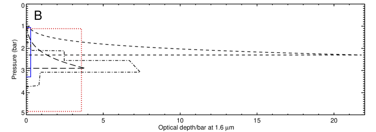
Figure 35.— Comparison of tropospheric cloud density vertical profiles on log scales (A) and linear scales (B). Our small-particle fit is shown with solid lines in both panels, while results from other investigators are shown using lines defined in the legend. The Irwin et al. (2015) result has been scaled downward by a factor of 10, which is a rough correction from what is shown in the left panel their Fig. 2, suggested by P.G.J. Irwin (personal communication). Their profile was derived for a deep methane mixing ratio of 1.6% and would move upward by several hundred mbar for double that mixing ratio. The Tice et al. (2013) profile was derived using a deep methane mixing ratio of 2.2%, which is also the case for the de Kleer et al. (2015) profile. As noted in the legend, our small-particle model has much less optical depth at 1.6 $\mu$m and much less total mass than the other results shown. The estimated total column cloud mass per unit area assumes a density of 1 g/cm³.

If these clouds are to be made of H₂S, it is worth considering whether there is enough H₂S available to make them. For a mixing ratio $\alpha_{H_{2}S}$, the mass per unit area of H₂S between two pressures separated by $\Delta$P would be (M${}_{H_{2}S}$/M)$\alpha_{H_{2}S}\Delta P/g$, where $g$ is gravity (9.748 m/s²), and the ratio of molecular weights of H₂S to the total is given by 34/2.3 = 14.78. For H₂S to condense at the tropospheric (layer-2) cloud base its mixing ratio must have a minimum value that depends on base pressure as shown in Fig. 36. To condense at the 3.3 bar level would require the H₂S VMR to be equal to its the solar mixing ratio of 3.1$\times 10^{-5}$ (Lodders, 2003). About 10 times that VMR would be needed to condense as deep as the 5 bar level and about ten times less would lead to condensation no deeper than the 2.4 bars. Microwave observations by de Pater et al. (1991) suggest H₂S is at least a factor of ten above solar. Even for just a 10 ppm mixing ratio, this yields an H₂S mass loading of 169 mg/cm² per bar of pressure difference. Thus, condensing all the H₂S in just a 1-bar interval would make 170 times the cloud mass that is inferred for the large-particle solution and more than 5000 times the mass needed for the small-particle cloud. Thus, none of these clouds is immediately ruled out by lack of condensable supply. A more sophisticated microphysical analysis would be needed to evaluate them, accounting for eddy mixing, coagulation, sedimentation, and other effects. Another test would be to compare model spectra for these various distributions with STIS spectra at CCD wavelengths. We have verified that our STIS-based models can fit near-IR spectra, but the reverse has not yet been demonstrated for near-IR based models.

Figure 36.— Minimum H₂S VMR required to condense at the cloud base versus cloud base pressure.

11. Summary and Conclusions

We observed Uranus with the HST/STIS instrument in 2015, following the same approach as in 2012 and 2002. We aligned the instrument’s slit parallel to the spin axis of Uranus and stepped the slit across the face of Uranus from the limb to the center of the planet, building up an image of half the disk with each of 1800 wavelengths from 300.4 to 1020 nm. The main purpose was to constrain the distribution of methane in the atmosphere of Uranus, taking advantage of the wavelength region near 825 nm where hydrogen absorption competes with methane absorption and displays a clear spectral signature. Our revised analysis approach used a considerably simplified cloud structure, relaxed the restriction that methane and thermal profiles should be consistent with radio occultation results, considered the new Uranus global mean profile of Orton et al. (2014a) that was inconsistent with radio occultation results, and included parameters defining the methane profile as part of the adjusted parameter sets in fitting observed spectra. This revised analysis applied to STIS observations of Uranus from 2015 and comparisons with similar 2002 and 2012 observations, as well as analysis of HST and Keck/NIRC2 imaging observations from 2007 and 2015, and IRTF SpeX spectra from 2013, have led us to the following conclusions.

1. TEMPORAL CHANGES

   • A direct comparison of 2012 STIS spectra with 2015 STIS spectra reveals no statistically significant difference at low latitudes. At 10^∘N and a zenith cosine of 0.7, the spectra from the two years are within the noise level of the measurements.

   • A different result is obtained by comparing 2012 and 2015 STIS spectra at high latitudes. There we find significant differences at pseudo-continuum wavelengths beyond 500 nm, where weaker methane bands are present, and where the 2015 I/F exceeds 2012 I/F values by up to 0.04 I/F units (about 15-20%). However, no difference is seen in the strong methane bands that would be sensitive to changes in stratospheric aerosols.

   • The brightening of high latitudes at pseudo continuum wavelengths between 2012 and 2015 is a result of increased scattering by tropospheric aerosols, and not due to a change in the effective methane mixing ratio. This is shown by radiation transfer modeling as well as by direct comparisons of imaging at wavelengths with different fractions of hydrogen and methane absorption.

   • The polar brightening from 2012 to 2015 that we found in comparisons of STIS spectra is part of a long-term trend evident from comparisons of H-band images from the 2007 equinox and onward, including recent images obtained in 2017 (Fry and Sromovsky, 2017).

2. METHANE DISTRIBUTION:

   • While the increased brightness of the polar region between 2012 and 2015 is due to increased aerosol scattering, the fact that the polar region is much brighter than low latitudes in 2015 is due to the lower mixing ratio of upper tropospheric methane at high latitudes.

   • We found that the STIS spectra from 2015 and 2012 can be well fit by relatively simple aerosol structures. We used a two-layer cloud structure with an optically thin stratospheric haze, and one tropospheric cloud, the latter extending from near 1 bar to several bars. This is similar to the 2-cloud model of Tice et al. (2013) except that we fit the upper boundary instead of fixing the upper boundary and fitting the scale height ratio. The particles in the tropospheric cloud were modeled either as spherical particles uniformly mixed with the gas and with a fitted real index, or as non-spherical particles using an HG phase function with a fitted asymmetry parameter.

   • Our initial fits to the 2015 STIS spectra over the entire range from 540 nm to 980 nm using either a two-cloud or three-cloud model using spherical particles of real refractive index of n = 1.4 produced good overall fits that were especially bad near 830 nm, just where the spectrum is especially sensitive to the methane to hydrogen ratio. Much better fits were obtained by allowing the refractive index of the tropospheric aerosols to be adjusted, which yielded two solutions, one a large-particle low-index solution and second small-particle high-index solution, the latter providing the better fit and somewhat closer match to the refractive index of H₂S.

   • Our preliminary 2-cloud models using spherical particles found little variation as a result of using different temperature profiles, as long as we did not force the deep methane mixing ratio or the methane humidity above the condensation level to be constrained either by occultation results or by a prohibition against supersaturation. We chose to use the Orton et al. (2014a) profile, even though it is inconsistent with occultation results, because its higher upper tropospheric temperatures allowed more methane without supersaturation.

   • For subsequent models containing a stratospheric haze and just a single tropospheric conservative Mie-scattering layer mixed uniformly with the gas, we did preliminary fits to spectra at 10^∘ N and 60^∘ N over the 730 nm to 900 nm range, and for both 2012 and 2015, assuming that methane was uniformly mixed below the condensation level. We found two classes of solutions, one with large particles of 1.1-1.75 $\mu$m in radius and a real index of 1.22$\pm$0.05 to 1.28$\pm$0.07, and a second solution set with small particles about 0.24$\pm$0.07 $\mu$m to 0.34$\pm$0.1 $\mu$m in radius with much larger real index values from 1.55$\pm$0.16 to 1.86$\pm$0.30. The small particle index values are much closer to that of H₂S, a prime candidate for the cloud’s main constituent.

   • The above preliminary fits with uniform methane mixing ratios found those ratios ranged from 2.56%$\pm$0.26% to 3.16%$\pm$0.5% at 10^∘N, and from 0.74%$\pm$0.05% to 0.99%$\pm$0.08% at 60^∘N, with lower values in both cases obtained from the large particle solutions, but good agreement between 2012 and 2015 in both cases.

   • Preliminary fits using non-spherical HG particles for the single tropospheric cloud layer produced similar results, with a methane mixing ratio from 2.85%$\pm$0.3% to 3.48%$\pm$0.5% at 10^∘N and from 0.97%$\pm$0.06% to 1.04%$\pm$0.07% at 60^∘N, and in this case differences between 2012 and 2015 are within estimated uncertainties.

   • All the above preliminary fits found methane humidities in the 68% to 95% at 10^∘N, and 30% to 56% at 60^∘N, generally with uncertainties of 12-16% and 18-26% respectively.

   • STIS results in the upper troposphere are in good agreement with the Lellouch et al. (2015) results based on Herschel observations. For 2015, the relative methane humidity above the nominal condensation level, which is roughly at the 1-bar level, for the Orton et al. thermal profile is roughly 50% north of 30^∘ N but near saturation from 20^∘ N and southward, but becomes supersaturated for the F1 and F0 profiles.

   • Latitude dependent fits assuming a uniform methane mixing ratio below the condensation level show that a local maximum value of about 3% is attained near 10^∘N latitude. From that point the effective mixing ratio smoothly declines by a factor of 2 by 45^∘N, and by a factor of three by 60^∘N, attaining a value of about 1% from 60^∘ to 70^∘N. However, if particle absorption is present, the derived mixing ratios are lowered by up to 10% of their values, or possibly more, depending on models. Thus, it is not possible to give a firm value of the mixing ratio without a deeper understanding to the aerosols within the atmosphere.

   • For a vertically uniform methane mixing ratio, the high-latitude model fits failed to accurately follow the observed spectra in the 750 nm region, suggesting that the upper tropospheric methane mixing ratio increased with depth. This was especially obvious for the 2012 observations, probably because of reduced aerosol scattering in 2012. A model profile containing a vertical gradient above the 5-bar level, using either what Sromovsky et al. (2011) called a descended depletion profile or a step decrease at the 3 bar level made a substantial improvement in the fit quality.

   • When the methane depletion with latitude is modeled as a stepped depletion, we find that the step change occurs at pressures between 3 and 5 bars, although the uncertainty is typically 2 bars. This level applies between about 50^∘ and 70^∘N, but moves to lower pressures between 50^∘ N and 20^∘ N, and remains near the condensation level from that point to 20^∘S. The mixing ratio above the break point pressure is near 0.75% in the 60^∘N to 70^∘N range, increasing to about 1.2% at low latitudes, although by that point the depleted layer is so thin that it is hard to distinguish from the uniformly mixed case with a single mixing ratio up to the condensation level.

   • Because the shape of the descended profile makes the depth parameter of that profile difficult to constrain with the spectral observations, we were guided by the stepped depletion results to choose a fixed depth parameter of 5 bars, and fit just the shape parameter $vx$ as a function of latitude. The results show a relatively smooth variation from slightly greater than 1 at high latitudes, increasing to about 4 by 30^∘N, then rising to very high values at low latitudes, which yields a nearly vertical profile that produces negligible depletion.

3. AEROSOL PROPERTIES:

   • Preliminary fits with non-spherical particles with a simple HG phase function yielded asymmetry parameters that ranged from 0.43$\pm$0.04 at 10^∘N to 0.26-0.39 at 60^∘N. These are smaller values than the commonly used value of $g$ = 0.7, e.g. by Tice et al. (2013). It is also smaller than the asymmetry parameters of even the small-particle solutions for the tropospheric aerosols, which ranged from about 0.4 at 1.6 $\mu$m to 0.6 at 0.8 $\mu$m. The large-particle asymmetry values were near 0.86 at 0.8 $\mu$m and 0.9 at 1.6 $\mu$m.

   • The cloud pressure boundaries varied with model structure. When a vertically uniform methane profile is assumed, the top boundary of the cloud is precisely constrained and nearly invariant with latitude, moving from slightly greater than 1 bar at low latitudes to almost exactly 1 bar at high latitudes. The lower boundary is more uncertain varying about a mean near 2.6 bars. The optical depth of the tropospheric cloud declines by roughly a factor of two from low to high latitudes, when 2012 and 2015 results are averaged. For the stepped depletion models, the top boundary behavior is similar to that of the uniform model, but the bottom boundary moves from 2.5 bars at low latitude to 3 bars at high latitude.

   • A very different characteristic is seen for the descended methane fits as a function of latitude. In this case the upper boundary of the tropospheric cloud moves significantly downward with latitude instead of slightly upward, with the pressure increasing from about 1.1 bar to 1.3 bar. We also found that the refractive index increased with latitude, from 1.6 to about 2.0, perhaps a result of a low-index coating evaporating from a high index core as the cloud descends to warmer temperatures. The particle radius also decreases somewhat with latitude, which would be consistent with that speculation. The tropospheric cloud optical depth is also seen to decline somewhat at high latitudes, as seen for other models.

   • The real refractive index of the main cloud has a relatively flat latitude dependence for the stepped depletion model, but significant increases with latitude are seen for uniform and descended depletion models. Better agreement is obtained at low latitudes, where weighted averages over 2012 and 2015 from 20^∘S to 20^∘N are 1.65$\pm$0.08, 1.66$\pm$0.07, and 1.63$\pm$0.07 for uniform, stepped depletion, and descended depletion models respectively, which are all above the expected value of 1.55 for H₂S by amounts that are not much greater than combined uncertainties.

   • The way aerosol contributions produce the increased polar brightness between 2012 and 2015 is simplest to understand within the context of the models assuming vertically uniform methane. In these cases an increased amount of scattering in the main cloud layer produces the brightness increase. And at 60^∘ N and 70^∘ N this is due to a combination of increased optical depth and increased particle size. Similar effects are seen in the stepped depletion model model (small particle solution). In the descended depletion model it appears that an increase in the cloud top pressure over time may be a significant factor. For the simple non-spherical HG particle cloud we found a 37% increase in optical depth coupled with a 33% decrease in the asymmetry parameter from 0.39 to 0.26. These effects would produce a combined rise in pseudo continuum I/F of about 32% (= 0.45$\times$(0.37+0.33)), which is comparable to the observed change.

   • The association of high-latitude methane depletions with descending motions of an equator-to-pole deep Hadley cell does not seem to be consistent with the behavior of the detected aerosol layers, at least if one ignores other cloud generation mechanisms such as sparse local convection. Both on Uranus and Neptune (de Pater et al., 2014), aerosol layers seem to form in what are thought to be downwelling regions on the basis of the effective methane mixing ratio determinations.

   • Models using conservative spherical particles in the tropospheric cloud layer have significant flaws when fit to the wider spectral range from 540 nm to 980 nm and assuming a real index of refraction of $n$ = 1.4. Much smaller flaws are seen with small particles with a larger refractive index, but more accurate fits require additional wavelength dependent scattering characteristics. This can be done by adding absorption in the longer wavelength regions, which allows increasing optical depths enough to brighten the shorter wavelength regions. For small particles with high real index values we needed to increase the imaginary index from zero at short wavelengths to 1.09$\times 10^{-3}$ between 670 to 730 nm and to 4.9$\times 10^{-2}$ from 730 nm to 1 $\mu$m. For non-spherical HG particles, we were able to match the same spectral region by creating an appropriate variation in optical depth with wavelength. It is also possible to produce a similar fit for DHG particles by appropriate wavelength dependence in the phase function, following an approach used by KT2009.

   • We were able to extend Mie model fits to the near-IR spectral range by further adjustments of the imaginary index with wavelength. For small particles the imaginary index had to be elevated to 0.1 at 1.6 $\mu$m, where its single-scattering albedo descends to 0.64. For large particles, the needed imaginary index increase was to a level eight times less than for small particles, and the single-scattering albedo was decreased to a more modest value of 0.90.

   • Our two solutions for cloud structures that can match spectra from visible to near-IR wavelengths to at least 1.6 $\mu$m, require vast differences in the total optical depth and cloud mass. These solutions bound solutions from other investigators, which have different vertical structures that in most cases match spectra from 0.8 to 1.6 $\mu$m. The column masses of particles in these clouds range from 500 to 17 times smaller than the total mass of H₂S in a 1-bar pressure interval, and thus, even the most massive of these clouds cannot be ruled out on the basis of insufficient parent condensate.

   • We found evidence for a deep cloud layer in the 9 bar to 11 bar range if optically thick and possibly composed of NH₄SH. Including this layer in our models has the main effect of improving our fits to the weak methane band structure at wavelengths from 540 nm to 600 nm. Placing the deep cloud at 5 bars yields an optical depth near 4 but a worse fit to the spectra. Further work is needed to better constrain the properties of this cloud.

4. CONSTRAINTS ON H₂S:

   • If the tropospheric cloud is a condensation cloud, H₂S is the likely main component. This conclusion is based on the fact that virtually all of the model cloud mass is below the level at which methane can condense, but likely within the pressure range at which H₂S can condense. It is also the case that our preferred small-particle solutions are in rough agreement with the refractive index of H₂S at low latitudes, although that agreement worsens at high latitudes and thus does not provide compelling support. More compelling support for H₂S as the main constituent of this cloud is the recent detection of H₂S vapor at saturation levels above this cloud (Irwin et al., 2018). What remains unclear is whether the spectrally varying imaginary index that seems to be required for this cloud is compatible with the absorbing properties of condensed H₂S.

   • Based on the estimated bottom boundary of the tropospheric aerosol layer, if the small particle solution is to be consistent with a composition of H₂S, the mixing ratio of H₂S at the 3.3-bar level and immediately below must be at least $\sim$30 ppm. To be consistent with the large particle solution would require around an order of magnitude higher VMR near the 5-bar level.

Advancing our understanding of the distribution and composition of Uranus’ aerosols would be helped by good measurements of the optical properties of H₂S, the most likely primary constituent of the most visible tropospheric cloud layer. Another helpful undertaking would be microphysical modeling of photochemical haze formation and seasonal evolution as well as microphysical modeling of condensation clouds. The variety of vertical aerosol structures and mass loadings that can produce model spectra matching the observations is surprisingly large and it seems likely that not all of these options would satisfy microphysical constraints. A better understanding of the aerosols is also the key to better constraints on the distribution of methane because different aerosol models yield different methane mixing ratios, with deep VMR values mostly falling between 2% and 4%. As Uranus seems to be continuing to change, especially the continued brightening of the north polar region through at least 2017, and many uncertainties remain, continued observations are also warranted.

Supplemental material.

The calibrated hyperspectral STIS cubes are archived at the Mikulski Archive for Space Telescopes (MAST) as High Level Science Products (HLSPs). They can be found at
https://archive.stsci.edu/prepds/uranus-stis/; https://dx.doi.org/10.17909/T9KQ4N. The 2015 cube is named hlsp_uranus-stis_hst_stis_uranus-2015_g430l-g750l_v1_cube.fits; 2002 and 2012 cubes are named analagously. The hyperspectral cubes contain calibrated I/F values as a function of wavelength and location, with navigation backplanes that provide viewing geometry and latitude-longitude coordinates for each pixel. A detailed explanation of the file contents is provided in the file README_SUPPLEMENTAL.TXT. A sample IDL program that reads a cube file, plots a monochromatic image, extracts data from a particular location on the disc, and plots a spectrum, is provided in the file stis_cube_example.pro. The IDL astronomy library will be needed to run the sample program.

NOTE: Until the MAST archive submission is finalized, which is underway at this writing and expected to be complete by the end of June 2018, the materials will be available for review at http://www.ssec.wisc.edu/planetary/ uranus/
onlinedata/ura2015stis/.

References

- Acton (1996) Acton, C. H., 1996. Ancillary data services of NASA’s Navigation and Ancillary Information Facility. Planet. and Space Sci. 44, 65–70.
- Borysow et al. (2000) Borysow, A., Borysow, J., Fu, Y., 2000. Semi-empirical model of collision-induced absorption spectra of H2-H2 complexes in the second overtone band of hydrogen at temperatures from 50 to 500 K. Icarus 145, 601–608.
- Colina et al. (1996) Colina, L., Bohlin, R. C., Castelli, F., 1996. The 0.12-2.5 micron Absolute Flux Distribution of the Sun for Comparison With Solar Analog Stars. Astron. J. 112, 307–315.
- Conrath et al. (1987) Conrath, B., Hanel, R., Gautier, D., Marten, A., Lindal, G., 1987. The helium abundance of Uranus from Voyager measurements. J. Geophys. Res. 92 (11), 15003–15010.
- Conrath et al. (1990) Conrath, B. J., Gierasch, P. J., Leroy, S. S., 1990. Temperature and circulation in the stratosphere of the outer planets. Icarus 83, 255–281.
- Conrath et al. (1991) Conrath, B. J., Pearl, J. C., Appleby, J. F., Lindal, G. F., Orton, G. S., Bézard, B., 1991. Thermal structure and energy balance of Uranus. Uranus, pp. 204–252.
- de Kleer et al. (2015) de Kleer, K., Luszcz-Cook, S., de Pater, I., Ádámkovics, M., Hammel, H. B., 2015. Clouds and aerosols on Uranus: Radiative transfer modeling of spatially-resolved near-infrared Keck spectra. Icarus 256, 120–137.
- de Pater et al. (2014) de Pater, I., Fletcher, L. N., Luszcz-Cook, S., DeBoer, D., Butler, B., Hammel, H. B., Sitko, M. L., Orton, G., Marcus, P. S., 2014. Neptune’s global circulation deduced from multi-wavelength observations. Icarus 237, 211–238.
- de Pater et al. (1991) de Pater, I., Romani, P. N., Atreya, S. K., 1991. Possible microwave absorption by H2S gas in Uranus’ and Neptune’s atmospheres. Icarus 91, 220–233.
- Fink and Sill (1982) Fink, U., Sill, G. T., 1982. The infrared spectral properties of frozen volatiles. In: Wilkening, L. L. (Ed.), IAU Colloq. 61: Comet Discoveries, Statistics, and Observational Selection. pp. 164–202.
- Friedson and Ingersoll (1987) Friedson, J., Ingersoll, A. P., 1987. Seasonal meridional energy balance and thermal structure of the atmosphere of Uranus - A radiative-convective-dynamical model. Icarus 69, 135–156.
- Fry and Sromovsky (2017) Fry, P. M., Sromovsky, L. A., 2017. Uranus’ post-equinox north polar brightening characterized with 2013 and 2016 IRTF SpeX observation. In: AAS/Division for Planetary Sciences Meeting Abstracts. Vol. 49 of AAS/Division for Planetary Sciences Meeting Abstracts. p. 115.17.
- Fry et al. (2012) Fry, P. M., Sromovsky, L. A., de Pater, I., Hammel, H. B., Rages, K. A., 2012. Detection and Tracking of Subtle Cloud Features on Uranus. Astron. J. 143, 150–161.
- Hanel et al. (1986) Hanel, R., Conrath, B., Flasar, F. M., Kunde, V., Maquire, W., Pearl, J., Pirraglia, J., Samuelson, R., Horn, L., Schulte, P., 1986. Infrared observations of the Uranian system. Science 233, 70–74.
- Hansen (1971) Hansen, J. E., 1971. Circular polarization of sunlight reflected by clouds. Journal of Atmospheric Sciences 28, 1515–1516.
- Havriliak et al. (1955) Havriliak, S., Swenson, R. W., Cole, R. H., 1955. Dielectric Constants of Liquid and Solid Hydrogen Sulfide. J. Chem. Phys. 23, 134–135.
- Hernandez et al. (2012) Hernandez, S., Aloisi, A., Bohlin, R., Bostroem, A., Diaz, R., Dixon, V., Ely, J., Goudfrooij, P., Hodge, P., Lennon, D., Long, C., Niemi, S., Osten, R., Proffitt, C., Walborn, N., Wheeler, T., York, B., Zheng, W., 2012. STIS Instrument Handbook, Version 12.0, (Baltimore: STScI). Space Telescope Science Institute, Baltimore, Maryland.
- Irwin et al. (2010) Irwin, P. G. J., Teanby, N. A., Davis, G. R., 2010. Revised vertical cloud structure of Uranus from UKIRT/UIST observations and changes seen during Uranus’ Northern Spring Equinox from 2006 to 2008: Application of new methane absorption data and comparison with Neptune. Icarus 208, 913–926.
- Irwin et al. (2015) Irwin, P. G. J., Tice, D. S., Fletcher, L. N., Barstow, J. K., Teanby, N. A., Orton, G. S., Davis, G. R., 2015. Reanalysis of Uranus’ cloud scattering properties from IRTF/SpeX observations using a self-consistent scattering cloud retrieval scheme. Icarus 250, 462–476.
- Irwin et al. (2018) Irwin, P. G. J., Toledo, D., Garland, R., Teanby, N. A., Fletcher, L. N., Orton, G. A., Bézard, B., 2018. Detection of hydrogen sulfide above the clouds in Uranus’s atmosphere. Nature Astronomy 2, 420–427.
- Karkoschka and Tomasko (2009) Karkoschka, E., Tomasko, M., 2009. The haze and methane distributions on Uranus from HST-STIS spectroscopy. Icarus 202, 287–309.
- Karkoschka and Tomasko (2010) Karkoschka, E., Tomasko, M. G., 2010. Methane absorption coefficients for the jovian planets from laboratory, Huygens, and HST data. Icarus 205, 674–694.
- Karkoschka and Tomasko (2011) Karkoschka, E., Tomasko, M. G., 2011. The haze and methane distributions on Neptune from HST-STIS spectroscopy. Icarus 211, 780–797.
- Khare et al. (1993) Khare, B. N., Thompson, W. R., Cheng, L., Chyba, C., Sagan, C., Arakawa, E. T., Meisse, C., Tuminello, P. S., 1993. Production and optical constraints of ice tholin from charged particle irradiation of (1:6) C2H6/H2O at 77 K. Icarus 103, 290–300.
- Krist (1995) Krist, J., 1995. Simulation of HST PSFs using Tiny Tim. In: Shaw, R. A., Payne, H. E., Hayes, J. J. E. (Eds.), Astronomical Data Analysis Software and Systems IV. Vol. 77 of Astronomical Society of the Pacific Conference Series. pp. 349–352.
- Lebofsky and Fegley (1976) Lebofsky, L. A., Fegley, Jr., M. B., 1976. Laboratory reflection spectra for the determination of chemical composition of ice bodies. Icarus 28, 379–387.
- Lellouch et al. (2015) Lellouch, E., Moreno, R., Orton, G. S., Feuchtgruber, H., Cavalié, T., Moses, J. I., Hartogh, P., Jarchow, C., Sagawa, H., 2015. New constraints on the CH4 vertical profile in Uranus and Neptune from Herschel observations. Astron. & Astrophys. 579, A121.
- Lindal et al. (1987) Lindal, G. F., Lyons, J. R., Sweetnam, D. N., Eshleman, V. R., Hinson, D. P., 1987. The atmosphere of Uranus - Results of radio occultation measurements with Voyager 2. J. Geophys. Res. 92, 14987–15001.
- Lodders (2003) Lodders, K., 2003. Solar System Abundances and Condensation Temperatures of the Elements. Astrophys. J. 591, 1220–1247.
- Orton et al. (1987) Orton, G. S., Aitken, D. K., Smith, C., Roche, P. F., Caldwell, J., Snyder, R., 1987. The spectra of Uranus and Neptune at 8-14 and 17-23 microns. Icarus 70, 1–12.
- Orton et al. (2014a) Orton, G. S., Fletcher, L. N., Moses, J. I., Mainzer, A. K., Hines, D., Hammel, H. B., Martin-Torres, F. J., Burgdorf, M., Merlet, C., Line, M. R., 2014a. Mid-infrared spectroscopy of Uranus from the Spitzer Infrared Spectrometer: 1. Determination of the mean temperature structure of the upper troposphere and stratosphere. Icarus 243, 494–513.
- Orton et al. (2014b) Orton, G. S., Moses, J. I., Fletcher, L. N., Mainzer, A. K., Hines, D., Hammel, H. B., Martin-Torres, J., Burgdorf, M., Merlet, C., Line, M. R., 2014b. Mid-infrared spectroscopy of Uranus from the Spitzer infrared spectrometer: 2. Determination of the mean composition of the upper troposphere and stratosphere. Icarus 243, 471–493.
- Rages et al. (1991) Rages, K., Pollack, J. B., Tomasko, M. G., Doose, L. R., 1991. Properties of scatterers in the troposphere and lower stratosphere of Uranus based on Voyager imaging data. Icarus 89, 359–376.
- Rannou et al. (1999) Rannou, P., McKay, C. P., Botet, R., Cabane, M., 1999. Semi-empirical model of absorption and scattering by isotropic fractal aggregates of spheres. Plan. & Sp. Sci. 47, 385–396.
- Sromovsky (2005a) Sromovsky, L. A., 2005a. Accurate and approximate calculations of Raman scattering in the atmosphere of Neptune. Icarus 173, 254–283.
- Sromovsky (2005b) Sromovsky, L. A., 2005b. Effects of Rayleigh-scattering polarization on reflected intensity: a fast and accurate approximation method for atmospheres with aerosols. Icarus 173, 284–294.
- Sromovsky and Fry (2007) Sromovsky, L. A., Fry, P. M., 2007. Spatially resolved cloud structure on Uranus: Implications of near-IR adaptive optics imaging. Icarus 192, 527–557.
- Sromovsky and Fry (2008) Sromovsky, L. A., Fry, P. M., 2008. The methane abundance and structure of Uranus’ cloud bands inferred from spatially resolved 2006 Keck grism spectra. Icarus 193, 252–266.
- Sromovsky and Fry (2010) Sromovsky, L. A., Fry, P. M., 2010. The source of 3-m absorption in Jupiter’s clouds: Reanalysis of ISO observations using new NH3 absorption models. Icarus 210, 211–229.
- Sromovsky et al. (2012a) Sromovsky, L. A., Fry, P. M., Boudon, V., Campargue, A., Nikitin, A., 2012a. Comparison of line-by-line and band models of near-IR methane absorption applied to outer planet atmospheres. Icarus 218, 1–23.
- Sromovsky et al. (2009) Sromovsky, L. A., Fry, P. M., Hammel, H. B., Ahue, W. M., de Pater, I., Rages, K. A., Showalter, M. R., van Dam, M. A., 2009. Uranus at equinox: Cloud morphology and dynamics. Icarus 203, 265–286.
- Sromovsky et al. (2012b) Sromovsky, L. A., Fry, P. M., Hammel, H. B., de Pater, I., Rages, K. A., 2012b. Post-equinox dynamics and polar cloud structure on Uranus. Icarus 220, 694–712.
- Sromovsky et al. (2011) Sromovsky, L. A., Fry, P. M., Kim, J. H., 2011. Methane on Uranus: The case for a compact CH4 cloud layer at low latitudes and a severe CH4 depletion at high latitudes based on re-analysis of Voyager occultation measurements and STIS spectroscopy. Icarus 215, 292–312.
- Sromovsky et al. (2014) Sromovsky, L. A., Karkoschka, E., Fry, P. M., Hammel, H. B., de Pater, I., Rages, K. A., 2014. Methane depletions in both polar regions of Uranus inferred from HST/STIS and Keck/NIRC2. Icarus 238, 137–155.
- Sun et al. (1991) Sun, Z., Schubert, G., Stoker, C. R., 1991. Thermal and humidity winds in outer planet atmospheres. Icarus 91, 154–160.
- Tice et al. (2013) Tice, D. S., Irwin, P. G. J., Fletcher, L. N., Teanby, N. A., Hurley, J., Orton, G. S., Davis, G. R., 2013. Uranus’ cloud particle properties and latitudinal methane variation from IRTF SpeX observations. Icarus 223, 684–698.
- Tomasko et al. (2005) Tomasko, M. G., Archinal, B., Becker, T., Bézard, B., Bushroe, M., Combes, M., Cook, D., Coustenis, A., de Bergh, C., Dafoe, L. E., Doose, L., Douté, S., Eibl, A., Engel, S., Gliem, F., Grieger, B., Holso, K., Howington-Kraus, E., Karkoschka, E., Keller, H. U., Kirk, R., Kramm, R., Küppers, M., Lanagan, P., Lellouch, E., Lemmon, M., Lunine, J., McFarlane, E., Moores, J., Prout, G. M., Rizk, B., Rosiek, M., Rueffer, P., Schröder, S. E., Schmitt, B., See, C., Smith, P., Soderblom, L., Thomas, N., West, R., 2005. Rain, winds and haze during the Huygens probe’s descent to Titan’s surface. Nature 438, 765–778.
- Tomasko et al. (2008) Tomasko, M. G., Doose, L., Engel, S., Dafoe, L. E., West, R., Lemmon, M., Karkoschka, E., See, C., 2008. A model of Titan’s aerosols based on measurements made inside the atmosphere. Plan. & Space Sci. 56, 669–707.