Halo structure of ¹⁷C

Abstract

¹⁷C has three states below the ¹⁶C + $n$ threshold with quantum numbers $J^{P}=3/2^{+},1/2^{+},5/2^{+}$. These states have relatively small neutron separation energies compared to the neutron separation and excitation energies of ¹⁶C. This separation of scales motivates our investigation of ¹⁷C in a Halo effective field theory (Halo EFT) with a ¹⁶C core and a valence neutron as degrees of freedom. We discuss various properties of the three states such as electric radii, magnetic moments, electromagnetic transition rates and capture cross sections. In particular, we give predictions for the charge radius and the magnetic moment of the $1/2^{+}$ state and for neutron capture on ¹⁶C into this state. Furthermore, we discuss the predictive power of the Halo EFT approach for the $3/2^{+}$ and $5/2^{+}$ states which are described by a neutron in a $D$-wave relative to the core.

I Introduction

Halo nuclei are weakly-bound states of a few valence nucleons and a tightly-bound core nucleus Zhukov et al. (1993); Hansen et al. (1995); Jonson (2004); Jensen et al. (2004); Riisager (2013). They exemplify the emergence of new degrees of freedom close to the neutron and proton drip lines which are difficult to describe in ab initio approaches. Cluster models of halo nuclei are formulated directly in the new degrees of freedom and thus take the emergence phenomenon into account by construction, typically using a phenomenological interaction Descouvemont (2008); Schuck et al. (2016). These models have improved our understanding of halo nuclei significantly. However, they cannot be improved systematically and lack a reliable way to estimate theoretical uncertainties.

Halo effective field theory (Halo EFT) is a systematic approach to these systems that exploits the apparent separation of scales between the small nucleon separation energy of the halo nucleus and the large nucleon separation energy and excitation energy of the core nucleus Bertulani et al. (2002); Bedaque et al. (2003). This scale separation defines (at least) two momentum scales: a small scale $M_{\text{lo}}$ and a large scale $M_{\text{hi}}$. Halo EFT provides a systematic expansion of low-energy observables in powers of $M_{\text{lo}}/M_{\text{hi}}$. Predictions made in Halo EFT can be improved systematically through the calculation of additional orders in the low-energy expansion. The interaction between the core and the valence nucleons is parametrized by contact interactions tuned to reproduce a few low-energy observables. Note that the absence of explicit pion exchange in the interaction indicates that the approach breaks down for momenta of the order of the pion mass. Similar EFT approaches can be used for systems of atoms and nucleons at low energies Braaten and Hammer (2006); Hammer and Platter (2010).

¹¹Be represents the prototype of a one-nucleon halo nucleus and thus has been considered as a test case for Halo EFT. It has a $J^{P}=1/2^{+}$ ground state that can be described as a neutron in an $S$-wave relative to the ¹⁰Be core. ¹¹Be also has a $J^{P}=1/2^{-}$ excited state which can be considered as a neutron in a $P$-wave relative to the core. The electric properties of the two bound states in ¹¹Be were studied in detail in Ref. Hammer and Phillips (2011) using Halo EFT. ¹¹Be also has a magnetic moment due to its halo neutron Fernando et al. (2015) but there are no magnetic transitions between the two states because of their opposite parity. For a recent review of Halo EFT and applications to other halo nuclei see Ref. Hammer et al. (2017).

Here, we will focus on the electromagnetic properties of ¹⁷C. This nucleus is an interesting halo candidate but has not yet been investigated using Halo EFT. Its continuum properties cannot yet be addressed using standard ab initio methods. It is too heavy for an approach that employs a combination of the no-core shell model (NCSM) and the resonating group model (RGM)Navrátil et al. (2016) but it is too light to neglect center-of-mass motion effects as is done in coupled cluster calculations. (See Ref. Hagen and Michel (2012) for a calculation of ⁴⁰Ca-proton scattering where this approximation is well justified.). Recent calculations in the NCSM also seem to suggest that this nucleus is too large to obtain converged results for its spectrum Smalley et al. (2015) with the available computational resources. ¹⁷C has a $J^{P}=3/2^{+}$ ground state, and two excited states with $J^{P}=1/2^{+}$ and $5/2^{+}$ Suzuki et al. (2008). The neutron separation energy of the ground state of about 0.7 MeV Wang et al. (2017) is significantly smaller than the excitation energy of the $J^{P}=0^{+}$ ¹⁶C core, which is about 1.8 MeV Ajzenberg-Selove (1986), while the neutron separation energies of the excited states are only of order 0.4-0.5 MeV Smalley et al. (2015) (see the level scheme in Fig. 1). This suggests that ¹⁷C may be amenable to a description using Halo EFT with $S$- and $D$-wave neutron-core interactions Braun et al. (2018).

Recently, M1 transition rates from both excited states into the ground state were measured Suzuki et al. (2008); Smalley et al. (2015). Below, we will discuss these transition rates in the framework of Halo EFT to leading order (LO) in the Halo EFT counting. Besides these electromagnetic transitions, we will also consider static electric and magnetic properties as well as neutron capture on ¹⁶C into ¹⁷C. We will show that future experiments and/or ab initio calculations of these quantities can provide insight in the interaction of neutrons with ¹⁶C.

This manuscript is organized as follows: In Sec. II, we introduce the theoretical foundations required to calculate the properties of halo nuclei with effective field theory. After reviewing results for the charge radius and quadrupole moment for the $S$- and $D$-wave states in Sec. III, we calculate magnetic moments for both states. In Sec. IV we discuss E2 and M1 transitions between the different states in ¹⁷C and calculate E1 and M1 capture reactions to the $S$- and $D$-wave states. We end with a summary and an outlook.

II Halo EFT formalism for ¹⁷C

Our goal is to investigate the electromagnetic properties of the halo nucleus ¹⁷C using Halo EFT. As discussed above, ¹⁷C can be described as a weakly-bound state of a ¹⁶C core and a neutron. First, we need to account for the free propagation of the core and neutron degrees of freedom. The corresponding Lagrangian is

$$\mathcal{L}_{0}=c^{\dagger}\left(i\partial_{t}+\frac{\nabla^{2}}{2M}\right)c+n^{\dagger}\left(i\partial_{t}+\frac{\nabla^{2}}{2m}\right)n\leavevmode\nobreak\ ,$$ (1)

where $n$ denotes the spin-1/2 neutron field, $c$ the spin-0 core field, $m$ is the nucleon mass, and $M$ is the mass of the ¹⁶C core.

Figure 1: Level scheme of ¹⁷C showing quantum numbers $J^{P}$, excitation energies in MeV, and the ¹⁶C$\leavevmode\nobreak\ +\leavevmode\nobreak\ n$ threshold.

The first excitation of the ¹⁶C core has an energy of $E_{{}^{16}C}^{*}=1.766(10)$ MeV Ajzenberg-Selove (1986), while the neutron separation energy of ¹⁶C is $S_{n}(^{16}{\rm C})=4.250(4)$ MeV Wang et al. (2017). Moreover, the neutron separation energy of ¹⁷C is $S_{n}(^{17}{\rm C})=0.734(18)$ MeV Wang et al. (2017). This suggests that the $J^{P}=3/2^{+}$ ground state of ¹⁷C can be described as a neutron in a $D$-wave relative to the ¹⁶C core, although the halo nature of the ground state is not commonly accepted Suzuki et al. (2008); Smalley et al. (2015). As illustrated in Fig. 1, ¹⁷C also has two excited states with $J^{P}=1/2^{+}$ and $5/2^{+}$ with energies $E^{*}_{1/2^{+}}=0.218(1)$ MeV and $E^{*}_{5/2^{+}}=0.332(1)$ MeV Smalley et al. (2015), respectively. In Halo EFT, these two states are described by a neutron in an $S$-wave and $D$-wave relative to the core, respectively. To account for these states, we define the interaction part of the effective Lagrangian as Braun et al. (2018)

$$\mathcal{L}=\mathcal{L}_{0} +d_{J,M}^{\dagger}\left[c_{2}^{J}\left(i\partial_{t}+\frac{\nabla^{2}}{2M_{nc}}\right)^{2}+\eta_{2}^{J}\left(i\partial_{t}+\frac{\nabla^{2}}{2M_{nc}}\right)+\Delta_{2}^{J}\right]d_{J,M}$$

$$-g^{J}_{2}\left[d^{\dagger}_{J,M}\left[n\overset{\leftrightarrow}{\nabla}^{2}c\right]_{J,M}+\left[n\overset{\leftrightarrow}{\nabla}^{2}c\right]^{\dagger}_{J,M}d_{J,M}\right]$$

$$+\sigma_{s}^{\dagger}\left[\eta_{0}\left(i\partial_{t}+\frac{\nabla^{2}}{2M_{nc}}\right)+\Delta_{0}\right]\sigma_{s}-g_{0}\left[c^{\dagger}n_{s}^{\dagger}\sigma_{s}+\sigma_{s}^{\dagger}n_{s}c\right]+\ldots\ ,$$ (2)

where $M_{nc}=M+m$ and $d_{J,M}$ is a $(2J+1)$-component field. We project on the $J=3/2$ and $5/2$ parts of the resonant $D$-wave interaction via

$$\left[n\overset{\leftrightarrow}{\nabla}^{2}c\right]_{J,M} =\sum_{m_{s}m_{l}}\left(\left.\frac{1}{2}m_{s}\ 2m_{l}\right|J\,M\right)\ n_{m_{s}}\sum_{\alpha\beta}\left(\left.1\alpha\ 1\beta\right|2m_{l}\right)\frac{1}{2}\left(\overset{\leftrightarrow}{\nabla}_{\alpha}\overset{\leftrightarrow}{\nabla}_{\beta}+\overset{\leftrightarrow}{\nabla}_{\beta}\overset{\leftrightarrow}{\nabla}_{\alpha}\right)\ c\ ,$$ (3)

where $\alpha$ and $\beta$ denote spherical indices and $\overset{\leftrightarrow}{\nabla}$ is a Galilei-invariant derivative. The $D$-wave interaction introduces 4 low-energy constants in the leading order (LO) Lagrangian: $c_{2}^{J}$, $\Delta_{2}^{J}$, $g^{J}_{2}$, and $\eta_{2}^{J}=\pm 1$, but only three of them are independent at LO. This increased number of parameters compared to the $S$-wave arises from the appearance of power divergences up to 5th order in the $D$-wave self-energy. Their renormalization requires effective range parameters up to the shape parameter to enter at LO Bertulani et al. (2002). In this work, we will follow Ref. Braun et al. (2018) and use dimensional regularization with the power divergence subtraction scheme (PDS) Kaplan et al. (1998a, b) for all practical calculations.

The accuracy of this approach is set by the ratio of the low-momentum scale $M_{\text{lo}}$ over the high-momentum scale $M_{\text{hi}}$ which for ground state observables can be estimated as $\sqrt{S_{n}(^{17}{\rm C})/E_{{}^{16}C}^{*}}\approx 0.64$ in our case. The expansion parameter is relatively large, and we expect slow convergence for ground state observables. However, for the excited states, the expansion parameter is approximately 0.5 which leads to 50% errors at first order and 25% errors at second order in the EFT expansion.

Figure 2: Diagrammatic representation of the dressed $d$-propagator. The dashed (solid) line denotes the core (neutron) field. The thin double line represents the bare $d$-propagator, while the thick double line with the blob is the dressed $d$-propagator.

The dressed propagators of the $\sigma$ and $d_{J,M}$ fields are obtained by summing the bubble diagrams for the $nc$-interactions (cf. Fig. 2 for the $D$-wave case) to all orders. Throughout this paper, a thick single line denotes the dressed $\sigma$-propagator and a thick double line the dressed $d$-propagator in all our figures.

$\sigma$-propagator. The $\sigma$-propagator for the $S$-wave state is well known (see, e.g., Ref. Hammer and Phillips (2011)) and we quote only the final result:

$$D_{\sigma}(\tilde{p}_{0}) =\frac{1}{\Delta_{0}+\eta_{0}[\tilde{p}_{0}+i\epsilon]-\Sigma_{\sigma}(\tilde{p}_{0})}\leavevmode\nobreak\ ,$$ (4)

$$\Sigma_{\sigma}(\tilde{p}_{0}) =-\frac{g^{2}_{0}m_{R}}{2\pi}\left[i\sqrt{2m_{R}\tilde{p}_{0}}+\mu\right]\leavevmode\nobreak\ ,$$ (5)

where $\mu$ is the PDS scale Kaplan et al. (1998a, b), $m_{R}$ the reduced mass of the neutron-core system, and $\tilde{p}_{0}=p_{0}-\mathbf{p}^{2}/(2M_{nc})$ is the Galilei invariant energy.

$d$-propagator. The dressed propagator for the $d_{J,M}$ field was computed in Ref. Braun et al. (2018). Since we use a Cartesian representation of the $D$-wave, the propagator depends on four vector indices, two in the incoming channel and two in the outgoing channel. Note that Roman indices refer to Cartesian indices and Greek ones to spherical indices. Evaluating the Feynman diagrams in Fig. 2, we obtain:

$$D_{d}(\tilde{p}_{0})_{ij,op}=D_{d}(\tilde{p}_{0})\ \frac{1}{2}\left(\delta_{io}\delta_{jp}+\delta_{ip}\delta_{jo}-\frac{2}{3}\delta_{ij}\delta_{op}\right)\ ,$$ (6)

$$D_{d}(\tilde{p}_{0})=\left[\Delta_{2}+\eta_{2}\tilde{p}_{0}+c_{2}\tilde{p}_{0}^{2}-\Sigma_{d}(\tilde{p}_{0})\right]^{-1}\ ,$$ (7)

with the one-loop self-energy

$$\Sigma_{d}(\tilde{p}_{0})=-\frac{2}{15}\frac{m_{R}g_{2}^{2}}{2\pi}\ (2m_{R}\tilde{p}_{0})^{2}\left[i\sqrt{2m_{R}\tilde{p}_{0}+i\epsilon}-\frac{15}{8}\mu\right]\ .$$ (8)

The term proportional to $c_{2}$ in (2) is required to absorb the $\mu$-dependence from the PDS scheme. Following the arguments in Ref. Braun et al. (2018), the terms proportional to $\eta_{2}$, $\Delta_{2}$, and $g_{2}$ are also required to be consistent with the threshold expansion of the scattering amplitude. In a momentum cutoff scheme, these terms absorb the linear, cubic, and quintic power law divergences in the cutoff Bertulani et al. (2002).

Power counting. The canonical power counting for the $\sigma$-propagator representing a shallow $S$-wave state was given in Refs. van Kolck (1997, 1999); Kaplan et al. (1998a, b). It implies $\gamma_{0}\sim 1/a_{0}\sim M_{\text{lo}}$ and $r_{0}\sim 1/M_{\text{hi}}$, where $\gamma_{0}=\sqrt{2m_{R}(S_{n}(^{17}\mathrm{C})-E^{*}_{{1/2}^{+}})}$ is the binding momentum of the $S$-wave state and $r_{0}$ the effective range. As a result, $r_{0}$ enters at NLO in the expansion in $M_{\text{lo}}/M_{\text{hi}}$.

The power counting for partial waves beyond the $S$-wave is more complicated and different scenarios have been proposed Bertulani et al. (2002); Bedaque et al. (2003); Braun et al. (2018). We look for a scenario that exhibits the minimal number of fine tunings consistent with the scales of the system. Bedaque et al. Bedaque et al. (2003) suggested for the $P$-wave case that $a_{1}\sim 1/(M_{\text{lo}}^{2}M_{\text{hi}})$ and $r_{1}\sim M_{\text{hi}}$, where higher ERE parameters scale with the appropriate power of $M_{\text{hi}}$ given by dimensional analysis. This power counting is adequate for the excited state of ¹¹Be Hammer and Phillips (2011). It requires only one fine-tuned constant in $\mathcal{L}$ instead of two as proposed in Ref. Bertulani et al. (2002) where both $a_{1}$ and $r_{1}$ scale with appropriate powers of $M_{\text{lo}}$. In Ref. Bedaque et al. (2003), the power counting was also generalized to $l>1$. However, we employ a different power counting with a minimal number of fine tunings for $l=2$ as proposed in Ref. Braun et al. (2018). In the case of the $d$-propagator, (6), two out of three ERE parameters need to be fine-tuned because $a_{2}\sim 1/(M_{\text{lo}}^{4}M_{\text{hi}})$ and $r_{2}\sim M_{\text{lo}}^{2}M_{\text{hi}}$ are both unnaturally large, while $\mathcal{P}_{2}\sim M_{\text{hi}}$. Higher ERE terms are suppressed by powers of $M_{\text{lo}}/M_{\text{hi}}$. Thus, the relevant fit-parameters in our EFT at LO are $\gamma_{0}$, $\gamma_{2}$, $r_{2}$, and $\mathcal{P}_{2}$, where $\gamma_{2}=\sqrt{2m_{R}S_{n}(^{17}\mathrm{C})}$ is the binding momentum of the ¹⁷C ground state, while $r_{2}$ and $\mathcal{P}_{2}$ denote the $D$-wave effective range and shape parameter, respectively. For the $5/2^{+}$ excited state, the binding momentum is $\gamma_{2^{\prime}}=\sqrt{2m_{R}(S_{n}(^{17}\mathrm{C})-E^{*}_{5/2^{+}})}$, while $r_{2^{\prime}}$, $\mathcal{P}_{2^{\prime}}$ are the corresponding effective range parameters.

The corresponding wave function renormalization constants for the $1/2^{+}$, $3/2^{+}$, and $5/2^{+}$ states at LO are:

$$Z_{\sigma}=\frac{2\pi}{m_{R}^{2}g_{0}^{2}}\ \gamma_{0}\ ,\qquad Z_{d}^{3/2}=-\frac{15\pi}{m_{R}^{2}g^{2}_{2}}\ \frac{1}{r_{2}+\mathcal{P}_{2}\gamma_{2}^{2}}\ ,\qquad Z_{d^{\prime}}^{5/2}=-\frac{15\pi}{m_{R}^{2}g^{2}_{2^{\prime}}}\ \frac{1}{r_{2^{\prime}}+\mathcal{P}_{2^{\prime}}\gamma_{2^{\prime}}^{2}}\ ,$$ (9)

respectively. At NLO, $Z_{\sigma}$ is modified by a factor $(1+\gamma_{0}r_{0})$. The constants $Z_{d}^{3/2}$ and $Z_{d^{\prime}}^{5/2}$ are only required at LO for our calculations.

III Static electromagnetic properties of ¹⁷C

We first consider the static electromagnetic properties of ¹⁷C. These are usually easier to measure experimentally than dynamical properties. They can also be calculated in ab initio approaches that provide the wave functions of the involved states. In particular, we will consider the charge radii and magnetic moments of the ¹⁷C states. It is convenient to calculate all form factors in the Breit frame where the photon transfers no energy, $q=(0,\boldsymbol{q})$, and to choose the photon to be moving in the $\hat{z}$ direction $\boldsymbol{q}=|\boldsymbol{q}|\hat{z}$.

III.1 Charge radii

The form factor of a general $S$-wave one-neutron halo nucleus was calculated in Ref. Hammer and Phillips (2011). The electric charge radius of the $S$-wave state at NLO is given by:

$$\braket{r_{E}^{2}}^{(\sigma)}=\frac{f^{2}}{2\gamma_{0}^{2}}(1+r_{0}\gamma_{0})\ .$$ (10)

where $f=m_{R}/M$ is a mass factor. The LO result can be obtained by setting $r_{0}=0$ in Eq. (10). At next-to-next-to-leading order (NNLO) a counterterm related to the radius of the core contributes. In the standard power counting, the factors of $f$ are counted as ${\cal O}(1)$, although they can become rather small for large core masses. As a consequence, the counterterm contribution is enhanced numerically. Up to NLO, one can interpret the Halo EFT result as a prediction for the radius relative to the core Hammer and Phillips (2011).

Using the measured one-neutron separation energy of the $1/2^{+}$ state, we obtain for the charge radius of the excited $S$-wave state of ¹⁷C relative to the charge radius of ¹⁶C at LO:

$$\braket{r_{E}^{2}}^{1/2^{+}}_{{}^{17}C}-\braket{r_{E}^{2}}_{{}^{16}C}=0.074\ \text{fm}^{2}\ ,$$ (11)

where the error from NLO corrections is about 50%. To make a numerical prediction for the full charge radius of ¹⁷C, we have to add the charge radius of ¹⁶C, $\braket{r_{E}^{2}}_{{}^{16}C}$, to our result. For this purpose, we use the point-proton radius $R_{p}$ from Ref. Kanungo et al. (2016) and the formula for the charge radius from Ref. Mueller et al. (2007), including the Darwin-Foldy term and the neutron charge radius as corrections, to obtain $\sqrt{\braket{r_{E}^{2}}^{1/2^{+}}_{{}^{17}C}}=\sqrt{\left(R_{p}^{{}^{16}C}\right)^{2}+r_{p}^{2}+\frac{3}{4m^{2}}+\frac{N}{Z}r_{n}^{2}+0.074\text{ fm}^{2}}=2.53(5)$ fm. Here we have used the proton, $r_{p}=0.875$ fm, and neutron charge radii, $r_{n}^{2}=-0.116$ fm² Yao et al. (2006), and $N=11$ ($Z=6$) denotes the number of neutrons (protons) of ¹⁷C. The error bar includes both the experimental and the Halo EFT uncertainties.

To date, there is no experimental data for the charge radius of the $1/2^{+}$ excited state to compare with. As a consistency check, we compare with the experimental value for the $3/2^{+}$ ground state of ¹⁷C extracted in Ref. Kanungo et al. (2016), $\sqrt{\braket{r_{E}^{2}}^{3/2^{+}}_{{}^{17}C}}=2.54(4)$ fm, which is very close to our result for the $1/2^{+}$ excited state. Note that the difference between the charge radius of ¹⁷C and ¹⁶C is smaller than the experimental error from Ref. Kanungo et al. (2016) for this quantity.

The charge radius of a $D$-wave state has recently been calculated in Ref. Braun et al. (2018) at LO and yields:

$$\braket{r_{E}^{2}}^{(d)}\ =-\frac{6\tilde{L}_{C0E}^{(d)\text{ LO}}}{r_{2}+\mathcal{P}_{2}\gamma_{2}^{2}}\ .$$ (12)

Here, the counterterm $\tilde{L}_{C0E}^{(d)\text{ LO}}$ already contributes at LO while the loop contribution is suppressed.

For the $D$-wave state, we also find a quadrupole moment which yields at LO:

$$\mu_{Q}^{(d)} =\frac{40\tilde{L}_{C02}^{(d)\text{ LO}}}{3\left(r_{2}+\mathcal{P}_{2}\gamma_{2}^{2}\right)}\ ,$$ (13)

where another counterterm enters at LO. Both $D$-wave observables have the same denominator of effective range parameters $(r_{2}+\mathcal{P}_{2}\gamma_{2}^{2})$ which is related to the Asymptotic Normalization Coefficient (ANC) of the $D$-wave state, $A_{2}=\sqrt{2\gamma_{2}^{4}/(-r_{2}-\mathcal{P}_{2}\gamma_{2}^{2})}$. Similar to the correlation between $\mu_{Q}^{(d)}$ and B(E2) in Ref. Braun et al. (2018), we find a smooth correlation between $\braket{r_{E}^{2}}^{(d)}$ and $\mu_{Q}^{(d)}$:

$$\mu_{Q}^{(d)}=-\frac{20}{9}\frac{\tilde{L}_{C02}^{(d)\text{ LO}}}{\tilde{L}_{C0E}^{(d)\text{ LO}}}\braket{r_{E}^{2}}^{(d)}\ ,$$ (14)

which implies that ab initio calculations with different phaseshift-equivalent interactions should show a linear correlation between the quadrupole moment and the charge radius.

III.2 Magnetic moments

Figure 3: Diagrams contributing to the magnetic moment. The first diagram is the coupling of a vector photon to the charge of the core arising from minimal substitution in the Lagrangian. The second diagram displays a vector photon coupling to the magnetic moment of the neutron. The last diagrams shows a two-body current. The thick solid line denotes the dressed $\sigma$-propagator.

The magnetic properties of shallow bound states are predominantly determined by the magnetic moments of its degrees of freedom. The magnetic moment of a single particle is introduced into the Lagrangian through an additional magnetic one-body operator Chen et al. (1999a); Fernando et al. (2015). An additional counterterm enters via a two-body current. Assuming a spin-0 core, the effective Lagrangian is

$$\mathcal{L}_{M}=\kappa_{n}\mu_{N}n^{\dagger}\boldsymbol{\sigma\cdot B}n+2\mu_{N}L_{M}^{J}\Phi^{\dagger}\boldsymbol{S_{J}\cdot B}\Phi\leavevmode\nobreak\ ,$$ (15)

where $\Phi$ is a place holder for the relevant auxiliary field ($\sigma_{s}$, $\pi_{s}$, $d_{J,M}$, …), $\boldsymbol{S_{J}}$ is the corresponding spin matrix for spin $J$, $\mu_{N}$ denotes the nuclear magneton, and $L^{J}_{M}$ the coupling constant for the magnetic two-body current. For the neutron anomalous magnetic moment we use $\kappa_{n}=-1.91304$.

III.2.1 Magnetic moment of the $1/2^{+}$ state

We reproduce the results obtained by Fernando et al. Fernando et al. (2015), who calculated electromagnetic form factors for $S$-wave states of one-neutron halo nuclei. Up to NLO, only the two last diagrams in Fig. 3 contribute to the magnetic form factor in the Breit frame:

$$\frac{eQ_{c}}{2M_{nc}}G_{M}(q^{2}) =Z_{\sigma}\mu_{N}\left(g_{0}^{2}\kappa_{n}\frac{mm_{R}}{\pi q}\arctan\left[\frac{qm_{R}}{2m\gamma_{0}}\right]+L_{M}^{\sigma}\right)\leavevmode\nobreak\ ,$$ (16)

with

$$Z_{\sigma}=\frac{2\pi\gamma_{0}}{m_{R}^{2}g_{0}^{2}}(1+r_{0}\gamma_{0})\leavevmode\nobreak\ ,\qquad\text{and we define}\qquad\tilde{L}_{M}^{\sigma}=\frac{2\pi L_{M}^{\sigma}}{m_{R}^{2}g_{0}^{2}}\ .$$ (17)

The magnetic moment $\kappa_{\sigma}$ is obtained by evaluating the form factor at $q^{2}=0$:

$$\kappa_{\sigma} =\frac{eQ_{c}}{2M_{nc}}G_{M}(0)=\left(\kappa_{n}+\tilde{L}_{M}^{\sigma}\gamma_{0}\right)(1+r_{0}\gamma_{0})\leavevmode\nobreak\ ,$$ (18)

where $\kappa_{\sigma}$ is given in units of $\mu_{N}$. Naive dimensional analysis with rescaled fields $[\tilde{\sigma}]=2$ Hammer and Phillips (2011) determines the scaling of the counterterm $\tilde{L}_{M}^{\sigma}\sim M_{\text{hi}}^{-1}$. As a consequence, $\tilde{L}_{M}^{\sigma}$ contributes at NLO. At LO, the magnetic moment of the $1/2^{+}$ state is thus given by the magnetic moment of the neutron, $\kappa_{n}$.

III.2.2 Magnetic moments of the $3/2^{+}$ and $5/2^{+}$ states

In the case of the $D$-wave, the only contribution to the magnetic moment at LO is the two-body current in Eq. (15), which corresponds to the last diagram in Fig. 3, and we obtain:

$$\frac{eQ_{c}}{2M_{nc}}G_{M}(q^{2}) =Z_{d}\mu_{N}L_{M}^{d}=-\frac{\mu_{N}\tilde{L}_{M}^{d}}{r_{2}+\mathcal{P}_{2}\gamma_{2}^{2}}\ ,$$ (19)

with

$$Z_{d}=-\frac{15\pi}{m_{R}^{2}g_{2}^{2}}\frac{1}{r_{2}+\mathcal{P}_{2}\gamma_{2}^{2}}\leavevmode\nobreak\ ,\qquad\text{and}\qquad\tilde{L}_{M}^{d}=\frac{15\pi L_{M}^{d}}{m_{R}^{2}g_{2}^{2}}\ .$$ (20)

This yields for the magnetic form factor at LO:

$$\kappa_{d}=-\frac{\tilde{L}_{M}^{d}}{{r_{2}+\mathcal{P}_{2}\gamma_{2}^{2}}}\leavevmode\nobreak\ ,$$ (21)

where $\kappa_{d}$ is again given in units of $\mu_{N}$. Beyond LO we also need to consider the two loop diagrams in Fig. 3. Therefore, we require additional counterterms to renormalize the corresponding divergences. This makes predictions even harder, and for that reason, we do not calculate the NLO contribution to the magnetic form factors for the $D$-wave state explicitly.

In general, the magnetic moment of the $D$-wave states will thus differ significantly from the magnetic moment of the neutron since $\kappa_{n}$ is a NLO contribution.

IV Electromagnetic transitions and capture reactions of ¹⁷C

IV.1 E2 transitions

The ground state and the two excited states of ¹⁷C have positive parity and differ at most by 2 units in total angular momentum. All states can therefore be connected by E2 transitions.

The transition strength for $S\rightarrow D^{\prime}$ has been calculated at LO in Ref. Braun et al. (2018) for the transition:

B(E2: $$1/2^{+}\to 5/2^{+} =-\frac{4}{5\pi}\frac{Z_{eff}^{2}e^{2}}{r_{2^{\prime}}+\mathcal{P}_{2^{\prime}}\gamma_{2^{\prime}}^{2}}\ \gamma_{0}\ \left[\frac{3\gamma_{0}^{2}+9\gamma_{0}\gamma_{2^{\prime}}+8\gamma_{2^{\prime}}^{2}}{(\gamma_{0}+\gamma_{2^{\prime}})^{3}}\right]^{2},$$) (22)

where the effective charge for ¹⁷C, $Z_{eff}=(m/M_{nc})^{2}Q_{c}\approx 0.021$ Typel and Baur (2005), comes out of the calculation automatically. At NLO, there is an unknown short-range contribution that enters via a counterterm.

For the transition strength B(E2: $1/2^{+}\to 3/2^{+}$), we get the same result for the amplitude but with different Clebsch Gordan coefficients (leading to a relative factor of $3/2$) and the appropriate binding momentum and renormalization constant for the $3/2^{+}$ ground state:

B(E2: $$1/2^{+}\to 3/2^{+} =-\frac{8}{15\pi}\frac{Z_{eff}^{2}e^{2}}{r_{2}+\mathcal{P}_{2}\gamma_{2}^{2}}\ \gamma_{0}\ \left[\frac{3\gamma_{0}^{2}+9\gamma_{0}\gamma_{2}+8\gamma_{2}^{2}}{(\gamma_{0}+\gamma_{2})^{3}}\right]^{2}.$$) (23)

Following the approach in Ref. Braun et al. (2018), we can also calculate the E2 transition for $D\to D^{\prime}$. However, we do not display the result here since the relevant diagram diverges cubically and, therefore, additional counterterms are required for this observable already at LO.

IV.2 M1 transitions

IV.2.1 S $\rightarrow$ D

We will first consider the M1 transition strength from the $3/2^{+}$ ground state ($D$-wave) to the first excited $1/2^{+}$ state ($S$-wave) in ¹⁷C since it was measured in Refs. Suzuki et al. (2008); Smalley et al. (2015). The experimental result is small compared with typical M1 transition strengths in nuclei, i.e. $\text{B(M1: $1/2^{+}\to 3/2^{+}$)}=1.04^{+0.03}_{-0.12}\times 10^{-2}\mu_{N}^{2}$ Smalley et al. (2015) or $0.58\times 10^{-2}$ W.U. expressed in Weisskopf units.

In the neutron-core picture of Halo EFT, the M1 transition from a $D$-wave to an $S$-wave state is forbidden for one-body currents which is in agreement with the experimental suppression of the transition. The non-zero transition strength can only be accounted for by a two-body current which takes short-ranged (core) physics into account. We therefore add the gauge-invariant counterterm

$$\mathcal{L}_{M}=-\mu_{N}L_{M1}^{\sigma d}\sigma_{m}^{\dagger}d_{m^{\prime}}\left(\frac{1}{2}m1i\bigg{|}\frac{3}{2}m^{\prime}\right)B_{i}\ .$$ (24)

By rescaling the fields to absorb unnaturally large coupling constants, leading to $[\tilde{\sigma}]=2$, $[\tilde{d}]=0$, and using naive dimensional analysis for the rescaled fields Beane and Savage (2001), we find $L_{M1}^{\sigma d}\sim M_{\text{hi}}l_{M1}^{\sigma d}g_{0}g_{2}m_{R}^{2}$ with $l_{M1}^{\sigma d}$ of order one. To obtain the magnetic transition amplitude we calculate the vertex function

$$\Gamma_{mm^{\prime}i}=\left(\frac{1}{2}m1i\bigg{|}\frac{3}{2}m^{\prime}\right)\mu_{N}\tilde{L}_{M1}^{\sigma d}\epsilon_{ijk}k_{j}\leavevmode\nobreak\ ,$$ (25)

with $\tilde{L}_{M1}^{\sigma d}=\frac{\sqrt{30}\pi}{m_{R}^{2}g_{0}g_{2}}L_{M1}^{\sigma d}$. If we consider the case $m=-m^{\prime}=\pm 1/2$ and choose the photon to be traveling in $\hat{z}$ direction, we find

$$\bar{\Gamma}_{\pm\mp,\mp 1}=\mp\frac{\mu_{N}}{\sqrt{3}}\tilde{L}_{M1}^{\sigma d}\omega\leavevmode\nobreak\ .$$ (26)

This yields for the M1 transition strength:

$$\text{B(M1: $1/2^{+}\to 3/2^{+}$)}=\frac{3}{4\pi}\left(\frac{\bar{\Gamma}_{\pm\mp,\mp 1}}{\omega}\right)^{2}=-\frac{1}{4\pi}\frac{\gamma_{0}}{r_{2}+\mathcal{P}_{2}\gamma_{2}^{2}}\left(\tilde{L}_{M1}^{\sigma d}\right)^{2}\mu_{N}^{2}\leavevmode\nobreak\ .$$ (27)

Moreover, combining Eqs. (27) and (23), we find a correlation between B(E2) and B(M1):

$$\text{B(E2: $1/2^{+}\to 3/2^{+}$)}=\frac{32}{15}\frac{Z_{eff}^{2}e^{2}}{\left(\tilde{L}_{M1}^{\sigma d}\right)^{2}\mu_{N}^{2}}\ \left[\frac{3\gamma_{0}^{2}+9\gamma_{0}\gamma_{2}+8\gamma_{2}^{2}}{(\gamma_{0}+\gamma_{2})^{3}}\right]^{2}\text{B(M1: $1/2^{+}\to 3/2^{+}$)}\leavevmode\nobreak\ .$$ (28)

If we use the experimental result for B(M1: $1/2^{+}\to 3/2^{+}$) $=1.04^{+0.03}_{-0.12}\times 10^{-2}\mu_{N}^{2}$ and employ naive dimensional analysis for the counterterm $\tilde{L}_{M1}^{\sigma d}\sim M_{\text{hi}}\approx 0.28\text{ fm}^{-1}$, we can make a rough prediction for B(E2),

$$\text{B(E2: $1/2^{+}\to 3/2^{+}$)}\approx 3\times 10^{-2}\ e^{2}\text{fm}^{4}\,.$$ (29)

Moreover, we can compare the M1 and E2 transition strengths for ¹⁷C if we look at the transition rates Greiner and Maruhn (1996),

$$T(R\lambda)=\frac{8\pi(\lambda+1)}{\lambda[(2\lambda+1)!!]^{2}}\omega^{2\lambda+1}B(R\lambda)\leavevmode\nobreak\ ,$$ (30)

that have, in contrast to B(M1) and B(E2), the same units. Here $R$ stands for E or M, $\lambda$ denotes the order of the transition and $\omega$ defines the photon energy which, in this case, is $0.218$ MeV (cf. Fig. 1). Using the naive dimensional analysis result for $\tilde{L}_{M1}^{\sigma d}$ from above we find:

$$\frac{T(E2)}{T(M1)}=\frac{32\omega^{2}}{125}\frac{Z_{eff}^{2}e^{2}}{\left(\tilde{L}_{M1}^{\sigma d}\right)^{2}\mu_{N}^{2}}\ \left[\frac{3\gamma_{0}^{2}+9\gamma_{0}\gamma_{2}+8\gamma_{2}^{2}}{(\gamma_{0}+\gamma_{2})^{3}}\right]^{2}\approx 1\times 10^{-5}\leavevmode\nobreak\ ,$$ (31)

which implies that the M1 transition strongly dominates over E2 for ¹⁷C.

IV.2.2 D’ $\rightarrow$ D

Figure 4: Relevant diagrams for the M1 transition. In the diagram (a) a vector photon couples to the magnetic moment of the neutron and in (b) to the electric charge of the core. In the two remaining diagrams the photon couples directly to the $D$-wave dimers. For a more detailed description of the lines, see Fig. 2.

The M1 transition strength from the $3/2^{+}$ ground state ($D$-wave) to the second excited $5/2^{+}$ state ($D^{\prime}$-wave) in ¹⁷C was also measured in Ref. Suzuki et al. (2008): $\text{B(M1: $5/2^{+}\to 3/2^{+}$)}=7.12_{-0.96}^{+1.27}\times 10^{-2}\mu^{2}_{N}$. Compared to the $D\to S$-state M1 transition strength, it is around one order of magnitude larger. This is in agreement with the fact that M1 transitions are allowed for neutron-core systems with one-body currents by the usual selection rules. We calculate both loop diagrams in Fig. 4 and find that we need additional counterterms to absorb all divergences. Moreover, we obtain results for the M3 and M5 transition. We find that two different counterterms are needed for the M1 transition and also two for the M3 transition.

In the following, we concentrate the discussion on the M1 transition. In this case, the two counterterms are given by:

$$\mathcal{L}_{M}=-L^{dd^{\prime}}_{M1a}\mu_{N}d^{\dagger}_{ij}d^{\prime}_{ij}\sigma_{k}^{m_{s}m_{s^{\prime}}}B_{k}\ -L^{dd^{\prime}}_{M1b}\mu_{N}d^{\dagger}_{ij}\boldsymbol{\nabla}\cdot{\bf A}d^{\prime}_{ij}\ .$$ (32)

The first counterterm is needed to renormalize the scale dependence from diagram (a) with the magnetic photon coupling to the neutron and the second one renormalizes the scale for the vector photon coupling in diagram (b), respectively. For the calculation it is convenient to define:

$$\tilde{L}_{M1a}^{dd^{\prime}} =\frac{15\pi}{m_{R}^{2}g_{2^{\prime}}g_{2}}L^{dd^{\prime}}_{M1a}+\frac{15}{4}\left(\gamma_{2}^{2}+\gamma_{2^{\prime}}^{2}\right)\kappa_{n}\mu\ ,$$ (33)

$$\tilde{L}^{dd^{\prime}}_{M1b} =\frac{15\pi}{m_{R}^{2}g_{2^{\prime}}g_{2}}L^{dd^{\prime}}_{M1b}+\frac{15}{4}\left(\gamma_{2}^{2}+\gamma_{2^{\prime}}^{2}\right)\frac{m_{R}Q_{c}}{M}\mu\ ,$$ (34)

where $\mu$ is the PDS scale.

Again, the photon has four-momentum $k=(\omega,\boldsymbol{k})$, and its polarization index is denoted by $\nu$. The computation of both diagrams yields a vertex function $\Gamma_{mm^{\prime}\nu}$ , where $m$ is the total angular momentum projection of the $3/2^{+}$ state and $m^{\prime}$ denotes the spin projection of the $5/2^{+}$ state. We compute the vertex function with respect to the specific components of the $D$-wave interaction:

$$\Gamma_{mm^{\prime}\nu}=\sum_{\alpha\beta\delta\eta m_{l}m_{l}^{\prime}m_{s}m_{s}^{\prime}}{\left(\frac{1}{2}m_{s}2m_{l}\left|\frac{3}{2}m\right.\right)\left(1\alpha 1\beta\left|2m_{l}\right.\right)\left(\frac{1}{2}m_{s}^{\prime}2m_{l}^{\prime}\left|\frac{5}{2}m^{\prime}\right.\right)\left(1\delta 1\eta\left|2m_{l}^{\prime}\right.\right)\tilde{\Gamma}_{\alpha\beta\delta\eta\nu}}\ .$$ (35)

We calculate the irreducible vertex in Coulomb gauge so that we have $\boldsymbol{k}\cdot\boldsymbol{\epsilon}=0$ for real photons. Additionally, we choose $\boldsymbol{k}\cdot\boldsymbol{p}=0$, where $\boldsymbol{p}$ denotes the incoming momentum of the $D$-wave state. As a result, the space-space components of the vertex function in Cartesian coordinates for the left diagram can be written as:

$$\tilde{\Gamma}_{ijopk}=\Gamma_{M}^{(a)}\epsilon_{abk}\sigma_{a}^{m_{s}m_{s^{\prime}}}k_{b}\left(\frac{\delta_{io}\delta_{jp}+\delta_{ip}\delta_{jo}}{2}-\frac{1}{3}\delta_{ij}\delta_{op}\right)\ ,$$ (36)

and for the right one:

$$\tilde{\Gamma}_{ijopk}=\Gamma_{M}^{(b)}p_{k}\left(\frac{\delta_{io}\delta_{jp}+\delta_{ip}\delta_{jo}}{2}-\frac{1}{3}\delta_{ij}\delta_{op}\right)+\Gamma_{E2}\left[k_{i}\left(\frac{\delta_{jp}\delta_{ko}+\delta_{jo}\delta_{kp}}{2}-\frac{1}{3}\delta_{jk}\delta_{op}\right)+\cdots\right]\ .$$ (37)

In the left diagram, the photon couples to the spin of the neutron and we get a spin flip $m_{s}\neq m_{s}^{\prime}$. In the case of the right diagram there is no spin flip so that $m_{s}=m_{s^{\prime}}$. By choosing the photon to be traveling in $\hat{z}$ direction it follows from the tensor structure of $\tilde{\Gamma}_{ijop\nu}$ that $m_{l}=m_{l}^{\prime}$ and $\nu\neq 0$. For the case that $m=\pm 1/2=-m^{\prime}$ we get:

$$-\Gamma_{-+,1}=\Gamma_{+-,-1}=\frac{\sqrt{6}}{5}\Gamma_{M}^{(a)}\sqrt{2}\omega\ ,$$ (38)

and for $m=m^{\prime}$ we get $0$ for all possible values. This yields for the B(M1: $3/2^{+}\to 5/2^{+}$) transition:

B(M1: $$3/2^{+}\to 5/2^{+} =\frac{3}{4\pi}\left(\frac{\Gamma_{+-,-1}}{\omega}\right)^{2}=\frac{9}{25\pi}\left(\frac{\bar{\Gamma}_{M}^{(a)}\omega}{\omega}\right)^{2}$$)

$$=\frac{9\mu_{N}^{2}}{25\pi}\frac{1}{r_{2}+\mathcal{P}_{2}\gamma_{2}^{2}}\frac{1}{r_{2^{\prime}}+\mathcal{P}_{2^{\prime}}\gamma_{2^{\prime}}^{2}}\left[\tilde{L}^{dd^{\prime}}_{M1a}+\frac{2\gamma_{2^{\prime}}^{4}\kappa_{n}}{\left(\gamma_{2^{\prime}}+\gamma_{2}\right)}+2\kappa_{n}\left(\gamma_{2}\gamma_{2^{\prime}}^{2}+\gamma_{2}^{3}\right)\right]^{2}\ ,$$ (39)

with the renormalized, irreducible vertex $\bar{\Gamma}_{M}=\sqrt{Z_{d}Z_{d^{\prime}}}\Gamma_{M}$. By rescaling the fields, $[\tilde{d}]=[\tilde{d}^{\prime}]=0$, and using dimensional analysis we find that the counterterm scales as $L^{dd^{\prime}}_{M1a}\sim M_{\text{hi}}^{3}l^{dd^{\prime}}_{M1a}g_{2}g_{2^{\prime}}m_{R}^{2}$ with $l^{dd^{\prime}}_{M1a}$ of order one. In contrast, the contribution from the loop scales as $M_{\text{lo}}^{3}$ which means that in LO only the counterterm contributes to the M1 transition and the loop diagram is suppressed by $(M_{\text{lo}}/M_{\text{hi}})^{3}$. Thus the M1 transition is strongly dominated by short-range physics.

IV.3 E1 neutron capture on ¹⁶C

IV.3.1 E1 capture into the $1/2^{+}$ state

E1 capture proceeds dominantly through the vector coupling of the photon to the halo core. The corresponding leading order operator is generated through minimal substitution in Eq. (2).

Figure 5: Relevant diagram contributing to the E1 capture amplitude to $S$-wave states at LO. For a more detailed description of the lines, see Fig. 2 and 3.

The diagram that contributes at LO to this process is shown in Fig. 5. It is the time-reversed diagram of the photodissociation reaction considered in Ref. Hammer and Phillips (2011). At LO, the amplitude is

$$\bar{\Gamma}^{i}=\frac{\boldsymbol{\epsilon^{i}\cdot p}}{M}\frac{\sqrt{Z_{\sigma}}eQ_{c}g_{0}2m_{R}}{\gamma_{0}^{2}+(\boldsymbol{p}-\frac{m}{M_{nc}}\boldsymbol{k})^{2}}\ ,$$ (40)

where $i$ is the photon polarization, $\boldsymbol{p}$ denotes the relative momentum of the $nc$ pair and $\boldsymbol{k}$ the photon momentum. Throughout this section we choose the $nc$ pair to be traveling in $\hat{z}$ direction which means that $\boldsymbol{p}=|\boldsymbol{p}|\boldsymbol{e}_{z}$. Since $m/M_{nc}$ is small and it follows from power counting that $p\sim\gamma_{0}\sim M_{\text{lo}}$ and $k\sim M_{\text{lo}}^{2}/M_{\text{hi}}$, we can neglect the recoil term $\sim\boldsymbol{p\cdot k}$ in the denominator. By averaging over the neutron spin and photon polarization and summing over the outgoing $S$-wave spin we obtain at LO ($\frac{m}{M_{nc}}k\ll p$):

$$\frac{d\sigma^{cap}}{d\Omega} =\frac{m_{R}}{4\pi^{2}}\frac{k}{p}|\mathcal{M}^{(1/2)}|^{2}\ =\ \frac{e^{2}Z_{eff}^{2}}{\pi m_{R}^{2}}\frac{p\gamma_{0}\sin^{2}{\theta}}{(p^{2}+\gamma_{0}^{2})}\ ,$$ (41)

with $k\approx(p^{2}+\gamma_{0}^{2})/2m_{R}$, $\bf\hat{k}\cdot\hat{p}=\cos\theta$, $Z_{eff}=(m_{R}/M)Q_{c}\approx 0.353$ and

$$|\mathcal{M}^{(1/2)}|^{2} =\frac{1}{2}\sum_{i,m_{s},M}|\bar{\Gamma}^{i}|^{2}\delta_{m_{s},M}\ ,$$ (42)

where $m_{s}$ denotes the neutron spin and $M$ the $S$-wave polarization. Since the neutron spin is unaffected by this reaction, $m_{s}$ and $M$ have to be the same. After integration over $d\Omega$ we get

$$\sigma^{cap} =\frac{m_{R}}{\pi}\frac{k}{p}|\mathcal{M}^{(1/2)}|^{2}\ =\ \frac{8e^{2}Z_{eff}^{2}}{3m_{R}^{2}}\frac{p\gamma_{0}}{(p^{2}+\gamma_{0}^{2})}=\ \frac{32\pi\alpha Z_{eff}^{2}}{3m_{R}^{2}}\frac{p\gamma_{0}}{(p^{2}+\gamma_{0}^{2})}\ ,$$ (43)

with the fine-structure constant $\alpha=e^{2}/(4\pi)$. Exploiting the detailed balance theorem, the capture cross section $\sigma^{cap}$ can be related to the photodissociation cross section $\sigma^{dis}$ Baur et al. (1986),

$$\sigma^{cap}=\frac{2(2j_{{}^{17}\text{C}}+1)}{(2j_{n}+1)(2j_{c}+1)}\frac{k^{2}}{p^{2}}\ \sigma^{dis}\ =\ 2\frac{k^{2}}{p^{2}}\ \sigma^{dis}\ .$$ (44)

Our numerical results for the E1 capture into ¹⁷C and photodissociation of ¹⁷C obtained using Eq. (44) at LO are shown in Fig. 6. At NLO, there is an additional contribution from the effective range $r_{0}$. By assuming that $r_{0}$ scales as $1/M_{\text{hi}}$, we can estimate the size of the NLO contribution by multiplying the LO result by a factor of $(1\pm\gamma_{0}/M_{hi})$ and add an error band to our LO results in Fig. 6.

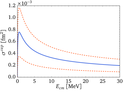
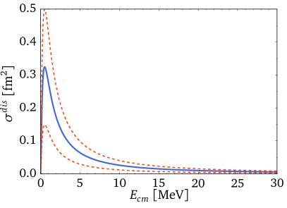
Figure 6: Left panel: E1 capture cross section into ¹⁷C as a function of the center-of-mass energy $E_{cm}$. Right panel: E1 photodissociation cross section as a function of $E_{cm}$. The solid (blue) line denotes the LO result and the dashed (red) lines show an estimate of the NLO corrections.

IV.3.2 E1 capture into the $3/2^{+}$ and $5/2^{+}$ states

Figure 7: Relevant diagrams for E1 capture to $D$-wave states at LO. For a more detailed description of the lines, see Fig. 2.

In this section, we calculate E1 neutron capture to the $3/2^{+}$ $D$-wave ground state and $5/2^{+}$ excited state of ¹⁷C. The relevant diagrams that emerge from minimal substitution in our Lagrangian (2) are shown in Fig. 7 . They yield

$$\bar{\Gamma}^{i}_{m_{s}JM} =\sum_{m_{s^{\prime}}m_{l}}\left(\left.\frac{1}{2}m_{s^{\prime}}\ 2m_{l}\right|J\,M\right)\sum_{\alpha\beta}\left(\left.1\alpha\ 1\beta\right|2m_{l}\right)\sqrt{Z_{d}}g_{2}eQ_{c}\frac{2m_{R}}{M}\times$$

$$\left[\frac{\left(\boldsymbol{p}-\frac{m}{M_{nc}}\boldsymbol{k}\right)_{\alpha}\left(\boldsymbol{p}-\frac{m}{M_{nc}}\boldsymbol{k}\right)_{\beta}}{\gamma_{2}^{2}+\left(\boldsymbol{p}-\frac{m}{M_{nc}}\boldsymbol{k}\right)^{2}}\ \boldsymbol{\epsilon^{i}\cdot p}+\epsilon^{i}_{\alpha}\left(p_{\beta}-\frac{m}{2M_{nc}}k_{\beta}\right)\right]\delta_{m_{s}m_{s}^{\prime}}\ ,$$ (45)

with the charge of the core $Q_{c}$, the photon momentum $\boldsymbol{k}$, the relative momentum of the incoming $nc$ pair $\boldsymbol{p}$, the photon polarization $i$ and $JM$ denoting the spin and polarization of the $D$-wave. Note that the neutron spin is unaffected by the E1 capture process up to this order. If we project out the $J=3/2$ part of the amplitude $M^{(3/2)}$ and average (sum) over incoming (outgoing) spins, respectively, we finally find the differential cross section for the E1 capture process at LO ($\frac{m}{M_{nc}}k\ll p$):

$$\frac{d\sigma^{cap}}{d\Omega} =\frac{m_{R}}{4\pi^{2}}\frac{k}{p}\left|\mathcal{M}^{(3/2)}\right|^{2}=\frac{15}{2\pi}\frac{\left(p^{2}+\gamma_{2}^{2}\right)}{m_{R}^{2}p}\frac{e^{2}Z_{eff}^{2}}{-r_{2}-\mathcal{P}_{2}\gamma_{2}^{2}}X(\theta)=\frac{30\alpha Z_{eff}^{2}}{-r_{2}-\mathcal{P}_{2}\gamma_{2}^{2}}\frac{\left(p^{2}+\gamma_{2}^{2}\right)}{m_{R}^{2}p}X(\theta)\ ,$$ (46)

with the fine-structure constant $\alpha$, $Z_{eff}=(m_{R}/M)Q_{c}$,

$$|\mathcal{M}^{(3/2)}|^{2}=\frac{1}{2}\sum_{i,m_{s},M}|\bar{\Gamma}^{i}_{m_{s}3/2M}|^{2}\ ,$$ (47)

and

$$X(\theta)=\frac{1}{15}\left[2p^{2}(13-\cos(2\theta))+\frac{4p^{4}\sin^{2}(\theta)}{\left(\gamma_{2}^{2}+p^{2}\right)}\left(\frac{p^{2}}{\left(\gamma_{2}^{2}+p^{2}\right)}+2\right)\right]\ .$$ (48)

After integrating over $d\Omega$ we find for the total cross section:

$$\sigma^{cap}=\frac{\alpha Z_{eff}^{2}}{-r_{2}-\mathcal{P}_{2}\gamma_{2}^{2}}\frac{32\pi p}{3m_{R}^{2}}\frac{\left(5\gamma_{2}^{4}+11p^{4}+14\gamma_{2}^{2}p^{2}\right)}{\left(\gamma_{2}^{2}+p^{2}\right)}\ .$$ (49)

From an experimental measurement of the capture (or dissociation) cross section we can therefore extract the numerical value of the combination of $D$-wave effective range parameters $1/(-r_{2}-\mathcal{P}_{2}\gamma_{2}^{2})$. For the $5/2^{+}$ state we project out the $J=5/2$ part of the amplitude $M^{(5/2)}$ and obtain:

$$\frac{d\sigma^{cap}}{d\Omega} =\frac{m_{R}}{4\pi^{2}}\frac{k}{p}\left|\mathcal{M}^{(5/2)}\right|^{2}=\frac{45}{4\pi}\frac{\left(p^{2}+\gamma_{2^{\prime}}^{2}\right)}{m_{R}^{2}p}\frac{e^{2}Z_{eff}^{2}}{-r_{2^{\prime}}-\mathcal{P}_{2^{\prime}}\gamma_{2^{\prime}}^{2}}X(\theta)=\frac{45\alpha Z_{eff}^{2}}{-r_{2^{\prime}}-\mathcal{P}_{2^{\prime}}\gamma_{2^{\prime}}^{2}}\frac{\left(p^{2}+\gamma_{2^{\prime}}^{2}\right)}{m_{R}^{2}p}X(\theta)\ ,$$ (50)

where $X(\theta)$ is the same as for the $J=3/2$ cross section. After integrating over $d\Omega$ we find for the total cross section:

$$\sigma^{cap}=\frac{\alpha Z_{eff}^{2}}{-r_{2^{\prime}}-\mathcal{P}_{2^{\prime}}\gamma_{2^{\prime}}^{2}}\frac{16\pi p}{m_{R}^{2}}\frac{\left(5\gamma_{2^{\prime}}^{4}+11p^{4}+14\gamma_{2^{\prime}}^{2}p^{2}\right)}{\left(\gamma_{2^{\prime}}^{2}+p^{2}\right)}\ ,$$ (51)

which is the same result as the $J=3/2$ cross section multiplied by a factor of $3/2$ and different numerical values for $\gamma_{2}$, $r_{2}$ and $\mathcal{P}_{2}$.

IV.4 M1 neutron capture on ¹⁶C

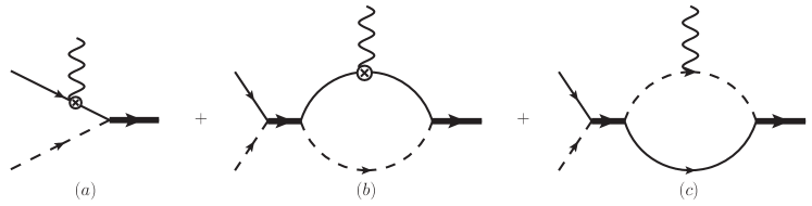
Figure 8: Relevant diagrams contributing to M1 capture at LO. For a more detailed description of the lines, see Fig. 2 and 3.

IV.4.1 M1 capture into the $1/2^{+}$ state

Similar to E1 capture, we can calculate the M1 capture cross section. The main difference between both processes is the parity conservation in the M1 matrix element. Therefore, the loop diagram (b) shown in Fig. 8 is also relevant at LO for M1 capture since initial state interactions in the $S$-wave channel have to be taken into account. Additionally, the photon now couples to the magnetic moment of the halo neutron in diagrams (a) and (b). In principle, we also need to consider diagrams which arise from minimal substitution. This is shown in the third diagram (c) where the photon couples to the charged ¹⁶C core. In the $S$-wave case, however, diagram (c) yields no contribution to the M1 capture process. For diagram (a) in Fig. 8 we get:

$$\bar{\Gamma}^{(a)}_{im_{s}m_{s^{\prime}}}=-2\sqrt{Z_{\sigma}}\kappa_{n}\mu_{N}g_{0}m_{R}\frac{\sigma_{j}^{m_{s}m_{s^{\prime}}}({\bf k}\times{\boldsymbol{\epsilon}^{i}})_{j}}{\gamma_{0}^{2}+\left(\boldsymbol{p}-\frac{M}{M_{nc}}\boldsymbol{k}\right)^{2}}\ ,$$ (52)

with the Pauli matrices $\sigma_{j}$, the photon polarization index $i$, and the relative momentum of the incoming $nc$ pair $\boldsymbol{p}$.

Since the power counting stipulates $p\sim\gamma_{0}\sim M_{\text{lo}}$ and $k\sim M_{\text{lo}}^{2}/M_{\text{hi}}$, we can neglect the recoil term $\sim\boldsymbol{p}\cdot{\bf k}$ in the denominator of Eq. (52).

$$\bar{\Gamma}^{(a)}_{im_{s}m_{s^{\prime}}}=-2\sqrt{2\pi\gamma_{0}}\kappa_{n}\mu_{N}\frac{\sigma_{j}^{m_{s}m_{s^{\prime}}}({\bf k}\times{\boldsymbol{\epsilon}^{i}})_{j}}{\gamma_{0}^{2}+p^{2}}\ .$$ (53)

Diagram (b) with the intermediate $S$-wave state yields

$$\bar{\Gamma}^{(b)}_{im_{s}m_{s^{\prime}}}=-\sqrt{Z_{\sigma}}g_{0}^{3}\kappa_{n}\mu_{N}\frac{2\pi}{g_{0}^{2}m_{R}}\frac{\sigma_{j}^{m_{s}m_{s^{\prime}}}({\bf k}\times{\boldsymbol{\epsilon}^{i}})_{j}}{\frac{1}{a_{0}}-\frac{r_{0}}{2}p^{2}+ip}\int{\frac{dl^{3}}{(2\pi)^{3}}\frac{2m_{R}}{p^{2}-l^{2}}\frac{2m_{R}}{\gamma_{0}^{2}+\left(\boldsymbol{l}+\frac{m_{R}}{m}\boldsymbol{k}\right)^{2}}}\ ,$$ (54)

with the loop momentum $\boldsymbol{l}$, which leads at LO to

$$\bar{\Gamma}^{(b)}_{im_{s}m_{s^{\prime}}}=2\sqrt{2\pi\gamma_{0}}\kappa_{n}\mu_{N}\frac{\sigma_{j}^{m_{s}m_{s^{\prime}}}({\bf k}\times{\boldsymbol{\epsilon}^{i}})_{j}}{\gamma_{0}+ip}\frac{1}{\gamma_{0}-ip}=-\bar{\Gamma}^{(a)}_{im_{s}m_{s^{\prime}}}\ .$$ (55)

As a consequence, both diagrams cancel each other at LO. In coordinate space, this process is given by an overlap integral between two orthogonal wave functions. At NLO, there is an additional contribution from the effective range $r_{0}$ as discussed for the E1 capture process before, which will give a correction of order $\gamma_{0}r_{0}\approx 40\%$. Moreover, a two-body current enters at NLO with an additional counter term that has to be fixed from data, similar to the case of magnetic moments discussed in Sec. III.2.1. This shows again that counter terms play a more dominant role in the magnetic sector than in the electric one.

Recoil corrections -

Subleading recoil corrections are usually dropped in EFT calculations for capture reactions such as this one. Taking recoil corrections into account, the first diagram (a) will give non-zero contributions to higher multipoles through higher partial waves in the initial state. The second diagram (b) in Fig. 8 contributes only when the core and the nucleon are in a relative $S$-wave in the initial state.

The denominator in Eq. (52) for diagram (a) can be spherically expanded as

$$\frac{1}{\gamma_{0}^{2}+\left(\boldsymbol{p}-\frac{M}{M_{nc}}\boldsymbol{k}\right)^{2}} =-\sum_{l}{(2l+1)i^{2l}P_{l}(\hat{p}\hat{k})\frac{M_{nc}}{2Mkp}\mathcal{R}e\bigg{\{}Q_{l}\left(-\frac{M_{nc}}{2Mpk}\left(p^{2}+\frac{M^{2}}{M_{nc}^{2}}k^{2}+\gamma_{0}^{2}\right)\right)\bigg{\}}}\ ,$$ (56)

where $Q_{l}(x)$ denotes the Legendre function of the second kind.

As an example, we consider the $S$-wave result for Eq. (56)

$$-\frac{1}{a}\ln\left(1-\frac{a}{\gamma_{0}^{2}+\left(p+\frac{M}{M_{nc}}k\right)^{2}}\right)\ ,$$ (57)

with $a=M_{nc}/(4Mkp)$, which is in perfect agreement with Eq. (53) if we set $k\sim 0$ and expand the logarithm.

After averaging and summing over incoming and outgoing spins, respectively, we obtain for the differential cross section the general result:

$$\frac{d\sigma^{cap}}{d\Omega}=\frac{m_{R}}{4\pi^{2}}\frac{k}{p}|\mathcal{M}^{(1/2)}|^{2}=\frac{m_{R}}{m^{2}}\frac{k^{3}}{p}\frac{4\alpha\kappa_{n}^{2}\gamma_{0}}{\left[\gamma_{0}^{2}+\left(\boldsymbol{p}-\frac{M}{M_{nc}}\boldsymbol{k}\right)^{2}\right]^{2}}\ ,$$ (58)

with the fine structure constant $\alpha$ and

$$|\mathcal{M}^{(1/2)}|^{2} =\frac{1}{2}\sum_{i,m_{s},m_{s^{\prime}}}|\bar{\Gamma}^{(a)}_{im_{s}m_{s^{\prime}}}|^{2}\ .$$ (59)

IV.4.2 M1 capture into the $3/2^{+}$ and $5/2^{+}$ states

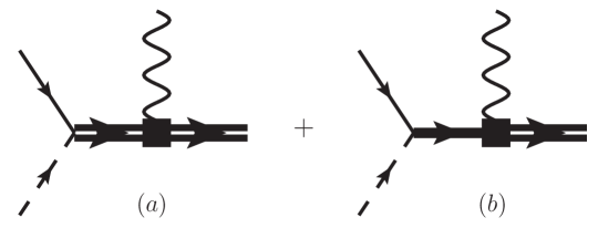
Figure 9: Relevant diagrams contributing to M1 capture into $D$-wave at up to NLO. The thick double line denotes the dressed $D$-wave dimer and the thick single line the dressed $S$-wave dimer. For a description of the other lines, see Figs. 2 and 3. The solid squares denote different vertices from two-body currents.

In this section, we calculate M1 neutron capture from the continuum into the $3/2^{+}$ $D$-wave ground state or $5/2^{+}$ excited state of ¹⁷C. Compared to the $1/2^{+}$ case in the previous section, there are additional contributions from two-body currents for the $D$-wave case at LO and NLO:

$$\mathcal{L}_{M}= -\mu_{N}L^{d^{\prime}d}_{M1cap}d^{\dagger}_{m^{\prime}}d^{\prime}_{m}B_{i}\left(\frac{5}{2}m1i\left|\frac{3}{2}m^{\prime}\right.\right)-\mu_{N}L^{dd}_{M1cap}d^{\dagger}_{m^{\prime}}d_{m}B_{i}\left(\frac{3}{2}m1i\left|\frac{3}{2}m^{\prime}\right.\right)$$

$$-\mu_{N}L^{d^{\prime}d^{\prime}}_{M1cap}d^{\prime\dagger}_{m^{\prime}}d^{\prime}_{m}B_{i}\left(\frac{5}{2}m1i\left|\frac{5}{2}m^{\prime}\right.\right)-\mu_{N}L^{\sigma d}_{M1cap}d^{\dagger}_{m^{\prime}}\sigma_{m}B_{i}\left(\frac{1}{2}m1i\left|\frac{3}{2}m^{\prime}\right.\right)\leavevmode\nobreak\ .$$ (60)

By rescaling the fields to absorb unnaturally large coupling constants, leading to $[\tilde{\sigma}]=2$, $[\tilde{d}]=[\tilde{d^{\prime}}]=0$, and using naive dimensional analysis for the rescaled fields Beane and Savage (2001), we find $L_{M1cap}^{d^{\prime}d}\sim M_{\text{hi}}^{3}l_{M1cap}^{d^{\prime}d}g_{2^{\prime}}g_{2}m_{R}^{2}$, $L_{M1cap}^{d^{(\prime)}d^{(\prime)}}\sim M_{\text{hi}}^{3}l_{M1cap}^{d^{(\prime)}d^{(\prime)}}g^{2}_{2^{(\prime)}}m_{R}^{2}$ and $L_{M1cap}^{\sigma d}\sim M_{\text{hi}}l_{M1cap}^{\sigma d}g_{0}g_{2}m_{R}^{2}$ with the constants $l_{M1cap}^{\cdots}$ all of order one. The corresponding diagrams are shown in Fig. 9. The first diagram (a) represents the first three terms in Eq. (60) where the two-body current is between two $D$-wave states. This is the LO contribution to the M1 capture process. The second diagram (b) belongs to the last term in Eq. (60) and is only relevant for the $3/2^{+}$ ground state. This yields an NLO contribution. The diagram (a) in Fig. 8, where the photon couples to the magnetic moment of the neutron, contributes at N²LO and the two loop diagrams at N³LO. Since we get additional counter terms $L_{M1cap}$ that have to be matched to data, predictions for the M1 capture in $D$-wave case become even more complicated. For that reason, we concentrate on the LO result which yields for the $5/2^{+}$ excited state:

$$\bar{\Gamma}_{m_{s}\frac{5}{2}M}^{i}=\sum_{m_{s}m_{l}}\left(\left.\frac{1}{2}m_{s}\ 2m_{l}\right|\frac{5}{2}M^{\prime}\right)\sum_{\alpha\beta}\left(\left.1\alpha\ 1\beta\right|2m_{l}\right)\frac{{p}_{\alpha}{p}_{\beta}}{\sqrt{r_{2^{\prime}}+\mathcal{P}_{2^{\prime}}\gamma_{2^{\prime}}^{2}}}\times$$

$$\mu_{N}\sum_{M^{\prime}\gamma}\left(\frac{5}{2}M^{\prime}1\gamma\left|\frac{5}{2}M\right.\right)({\bf k}\times{\boldsymbol{\epsilon}^{i}})_{\gamma}\ \frac{\tilde{L}_{M1cap}^{d^{\prime}d^{\prime}}}{\frac{1}{a_{2^{\prime}}}-\frac{r_{2^{\prime}}}{2}p^{2}+\frac{\mathcal{P}_{2^{\prime}}}{4}p^{4}}\ ,$$ (61)

with the $D$-wave polarizations $\alpha$ and $\beta$, the photon momentum $\boldsymbol{k}$, photon polarization $i$, the relative momentum of the incoming $nc$ pair $\boldsymbol{p}$, and we have defined $\tilde{L}_{M1cap}^{d^{\prime}d^{\prime}}=\frac{(15\pi)^{3/2}}{m_{R}^{2}g_{2^{\prime}}^{2}}L_{M1cap}^{d^{\prime}d^{\prime}}$. For the $3/2^{+}$ ground state we obtain:

$$\bar{\Gamma}_{m_{s}\frac{3}{2}M}^{i}=\left(\left.1\alpha\ 1\beta\right|2m_{l}\right)\frac{{p}_{\alpha}{p}_{\beta}\mu_{N}({\bf k}\times{\boldsymbol{\epsilon}^{i}})_{\gamma}}{{\sqrt{r_{2}+\mathcal{P}_{2}\gamma_{2}^{2}}}}\left[\left(\left.\frac{1}{2}m_{s}\ 2m_{l}\right|\frac{3}{2}M^{\prime}\right)\left(\frac{3}{2}M^{\prime}1\gamma\left|\frac{3}{2}M\right.\right)\frac{\tilde{L}_{M1cap}^{dd}}{\frac{1}{a_{2}}-\frac{r_{2}}{2}p^{2}+\frac{\mathcal{P}_{2}}{4}p^{4}}\right.$$

$$+\left.\left(\left.\frac{1}{2}m_{s}\ 2m_{l}\right|\frac{5}{2}M^{\prime}\right)\left(\frac{5}{2}M^{\prime}1\gamma\left|\frac{3}{2}M\right.\right)\frac{\tilde{L}_{M1cap}^{d^{\prime}d}}{\frac{1}{a_{2^{\prime}}}-\frac{r_{2^{\prime}}}{2}p^{2}+\frac{\mathcal{P}_{2^{\prime}}}{4}p^{4}}\right]\ ,$$ (62)

where we have implicitly summed over repeated indices and we have defined $\tilde{L}_{M1cap}^{dd}=\frac{(15\pi)^{3/2}}{m_{R}^{2}g_{2}^{2}}L_{M1cap}^{dd}$ and $\tilde{L}_{M1cap}^{d^{\prime}d}=\frac{(15\pi)^{3/2}}{m_{R}^{2}g_{2^{\prime}}g_{2}}L_{M1cap}^{d^{\prime}d}$. The differential cross section for the M1 capture process at LO for $J=3/2$ or $5/2$ is then given by:

$$\frac{d\sigma^{cap}}{d\Omega}=\frac{m_{R}}{4\pi^{2}}\frac{k}{p}|\mathcal{M}^{(J)}|^{2}\leavevmode\nobreak\ ,\quad\text{with}\quad|\mathcal{M}^{(J)}|^{2} =\frac{1}{2}\sum_{i,m_{s},M}|\bar{\Gamma}_{m_{s}JM}^{i}|^{2}\ .$$ (63)

Since we need at least four additional input parameters to make predictions for the M1 capture process into the $D$-wave state already at LO, numerical predictions are currently not possible. This shows the limitations of Halo EFT for higher partial waves especially in the magnetic sector.

V Summary

Halo nuclei are weakly bound systems of a tightly bound core nucleus and a small number of valence nucleons. Their structure can be probed experimentally by measuring capture reactions, dissociation cross sections, and charge radii. In this work, we have discussed these observables for $S$- and $D$-wave halo states using the framework of Halo EFT.

We have considered the nucleus ¹⁷C as a halo nucleus consisting of a ¹⁶C core and a neutron. ¹⁷C is an interesting halo candidate since it has three $S$- and $D$-wave neutron-core states with small neutron separation energies in its spectrum. We have calculated the key observables relevant to this system, including radii, magnetic moments as well as electric and magnetic transition rates. Moreover, we showed that capture reactions can provide insight into the continuum properties of the neutron-¹⁶C system.

We found that predictions of many observables for states with angular momentum larger than zero need additional input parameters, beyond the neutron separation energy. This limits the predictive power of Halo EFT for such states. However, these counterterms can be matched to experiment or other theoretical calculations. For example, the counterterms appearing in the expressions for the $S$- to $D$-wave transitions can be determined in this way. Coupled-cluster calculations for ¹⁷C were carried out in Ref. Kanungo et al. (2016) using effective interactions derived from first principles, and this approach could be extended to calculate the transitions in our work. The results could then be used to predict capture cross sections since the counterterms in capture cross sections and transition strengths are related. This strategy would provide insights into the continuum properties of ¹⁷C based on a combination of halo EFT and the shell model. Alternatively, one can eliminate unknown counterterms by considering correlations between different observables. These correlations can be used to test the consistency between different ab initio calculations and/or experimental data. The structure of such correlations is universal in the sense that it is independent of the specific neutron separation energies and applies to all states with the same quantum numbers. As a consequence, Halo EFT is complementary to ab initio approaches by exploiting universal correlations driven by the weak binding.

Some of the observables discussed in this work have been studied extensively in the case of the deuteron which can be considered the lightest halo nucleus, consisting of a neutron and a proton core Chen et al. (1999a, b). One-neutron halo nuclei can therefore have similar electromagnetic properties to the deuteron. For example, the expression for the LO charge radius of an $S$-wave neutron halo nucleus shown in Eq. (10) is the same as for the deuteron. However, the deuteron consists of two spin-1/2 particles and interacts resonantly in the spin-triplet and spin-singlet $S$-wave channels. This leads to a relatively large M1 capture cross section between the unbound spin-singlet and the spin-triplet channel in which the deuteron resides. The absence of a second resonantly interacting channel leads a strong suppression of magnetic capture in the case of ¹⁷C.

We hope that our investigation will motivate further theoretical and experimental investigations of ¹⁷C. The expressions presented in this paper should be useful for the analysis of experimental and/or ab initio data on ¹⁷C in order to establish the halo nature of ¹⁷C. The combination of Halo EFT and ab initio calculations as was done in Refs. Hagen et al. (2013); Ryberg et al. (2014); Zhang et al. (2014) could provide insights into the continuum properties of ¹⁷C and should facilitate a test of the power counting that was used in this work.

Future extensions of our calculation to NLO and beyond would improve this comparison quantitatively, but a growing number of counterterms may invalidate this advantage.