Extended Creutz ladder with spin-orbit coupling: a one-dimensional analog of the Kane-Mele model

Abstract

We construct a topological ladder model, one-dimensional, following the steps which lead to the Kane-Mele model in two dimensions. Starting with a Creutz ladder we modify it so that the gap closure points can occur at either $k=\pi/2$ or $-\pi/2$. We then couple two such models, one for each spin channel, in such a way that time-reversal invariance is restored. We also add a Rashba spin-orbit coupling term. The model falls in the CII symmetry class. We derive the relevant $2\mathbb{Z}$ topological index, calculate the phase diagram and demonstrate the existence of edge states. We also give the thermodynamic derivation of the quantum spin Hall conductance (Středa-Widom). Approximate implementation of this result indicates that this quantity is sensitive to the topological behavior of the model.

I Introduction

Topological systems Hasan10 are one of the most active current research areas in condensed matter physics. A crucial advance in this field was the Haldane model Haldane88 (HM), a hexagonal model in which time-reversal symmetry and inversion symmetry are simultaneously broken. The model is engineered so that a gap can be closed at either one of the Dirac points. The gap closure occurs at a phase line, which encloses a topological phase with finite Hall conductance, whose sign depends on which gap is closed at the phase line. An extension of the HM, the Kane-Mele model Kane05a ; Kane05b (KMM), was another important step in the development of topological insulators. In this model two Haldane models are taken, one for each spin channel, each one tuned so that time-reversal symmetry is restored. A Rashba coupling term, which mixes different spins, is also added. The KMM model exhibits quantized quantum spin Hall (QSH) response, and sustains spin currents at its edges.

Topological models in one dimension Su79 ; Rice82 ; Creutz94 ; Creutz99 ; Kitaev01 ; Li13 ; Li14 ; Wakatsuki14 ; Atherton16 ; Hetenyi18 are also actively studied. Of the many such models, most relevant to our study is the Creutz model Creutz94 ; Creutz99 which exhibits a topological interference effect which can be probed when open boundary conditions are applied (edge-states). Recent studies Sticlet13b ; Sticlet13 ; Viyuela14 ; Bermudez09 of this model revealed several interesting phenomena. The Uhlmann phase was used Viyuela14 as a measure of topological behavior at finite temperature. It was also shown Bermudez09 that defect production across a critical point obeys non-universal scaling depending on the topological features. We also emphasize that a number of different one-dimensional topological models Li13 ; Hetenyi18 exhibit the same phase diagram as the HM.

Topological ladder models Strinati17 ; Sun12 are one-dimensional systems which, however, often exhibit effects usually associated with two dimensions. Strinati et al. Strinati17 recently showed that ladder models can support Laughlin-like states with chiral current flowing along the legs of the ladder. Since a ladder consists of two legs separated by a finite distance, and enclosing a definite area, it is possible to apply a magnetic field perpendicular to this area and observe a quantum Hall response. Another way to think about this is to realize that to demonstrate the existence of chiral edge currents, one needs a strip, which is also an effective one-dimensional system, with a finite width (a ladder is a strip with width of one, or a small number of, lattice constants). Recently Hetenyi18 we demonstrated that a ladder model can be constructed to exhibit topological effects similar to the HM. Our interest here is whether it is possible to also construct a ladder in the spirit of KMM.

In this paper we construct a ladder model, step-by-step, which can be viewed as the one-dimensional analog of the KMM. First, we modify the original Creutz model so that gap closures are shifted in $k$-space, breaking time-reversal invariance. We then couple two such shifted Creutz models, one for each spin channel, so that time-reversal invariance is restored. We also add a Rashba term to allow for the mixing of spins. We then derive a topological winding number for the model, and calculate its phase diagram. We also use the Widom derivation of the QSH formula, which gives quantized response in the topological region. The possible experimental signature is spin currents flowing along the legs of the ladder.

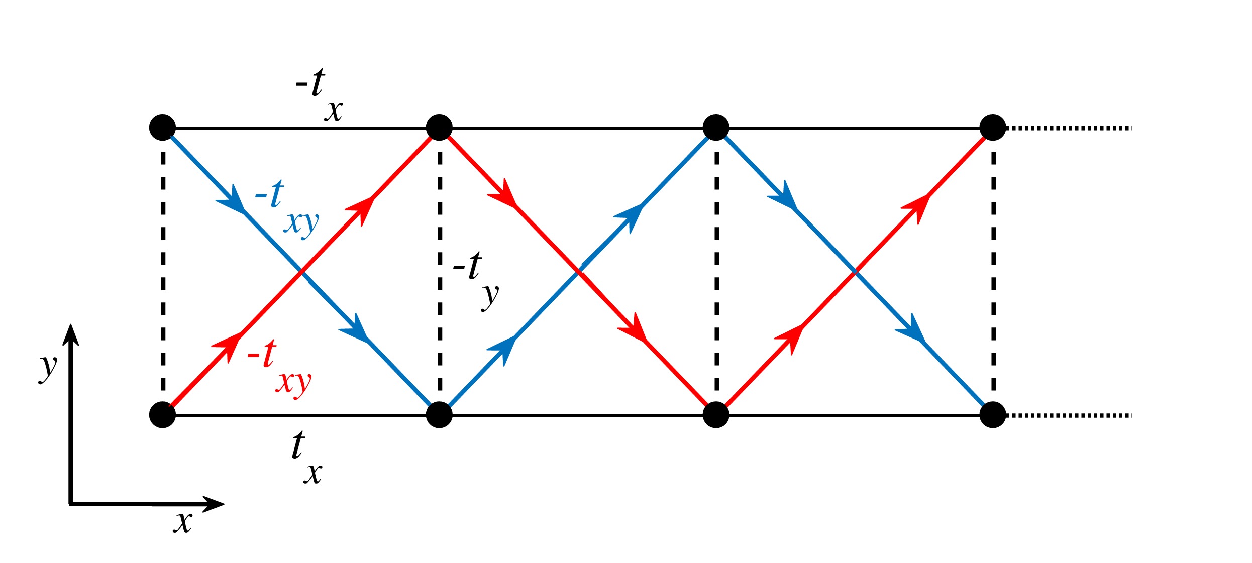
Figure 1: Graphic representation of our model. $t_{x}$($t_{y}$) denotes hoppings along horizontal(vertical) bonds. $t_{xy}$ denotes diagonal bonds. We apply Peierls phases along the diagonal bonds along the directions indicated.

II Models

The Creutz model is a quasi-1D ladder model which exhibits a quantum phase transition separating a trivial phase from a symmetry-protected topological phase. The topological phase is characterized by a winding number, and if open boundary conditions are applied, localized edge states are found. Let $t_{x}$ denote hoppings along the legs, $t_{y}$ the hoppings perpendicular to the legs, and $t_{xy}$ the diagonal hoppings along unit cells. In the original Creutz model a magnetic field perpendicular to the plane of the system is applied, resulting in Peierls phases along the legs of the ladder, pointing in opposite directions on different legs of the ladder. For a Peierls phase of $\pi/2$ the resulting Hamiltonian is

$$H_{C}=-\sum_{k}[(2t_{x}\sin(k))\hat{\sigma}_{z}+(t_{y}+2t_{xy}\cos(k)\hat{\sigma}_{x})].$$ (1)

Gap closure occurs at the points $k=0,\pi$, depending on whether $t_{y}=2t_{xy}$ or $t_{y}=-2t_{xy}$. Our first step is to set the bonds on the upper(lower) leg to $t_{x}$($-t_{x}$) and introduce Peierls phases of $\pi/2$ on the diagonal bonds as indicated in Fig. 1. The Hamiltonian is now

$$H_{1}=-\sum_{k}[(2t_{x}\cos(k))\hat{\sigma}_{z}+(t_{y}+2t_{xy}\cos(k+\Phi)\hat{\sigma}_{x})].$$ (2)

The first term alone corresponds to a band stucture with one-dimensional Dirac points at $k=\pm\pi/2$, which are time-reversal invariant pairs. The second term opens gaps in general with masses of opposite signs at opposite Dirac points. The phase diagram (determined by the gap closure condition) is the same as that of the HM,

$$\frac{t_{y}}{2t_{xy}}=\pm\sin(\Phi).$$ (3)

The sign in Eq. (3) determines which of the two gaps in the Brillouin zone closes.

Given that the gap closures occur at time-reversal invariant points, we can proceed to construct a one-dimensional analog of the Kane-Mele model, by first introducing spin,

$$H_{2}=\sum_{k}d_{1}(k)\Gamma^{(1)}+d_{2}(k)\Gamma^{(2)}+d_{25}(k)\Gamma^{(25)},$$ (4)

where we have used the following $\Gamma$-matrices,

$$\Gamma^{(a)}=\{\sigma_{x}\otimes I_{2},\sigma_{z}\otimes I_{2},\sigma_{y}\otimes\sigma_{x},\sigma_{y}\otimes\sigma_{y},\sigma_{y}\otimes\sigma_{z}\},$$ (5)

with $a=1,...,5$, and

$$\Gamma^{(ab)}=\frac{1}{2i}[\Gamma^{(a)},\Gamma^{(b)}],$$ (6)

$H_{2}$ can be viewed as the “square” of the $H_{1}$ Hamiltonian. We can now add the Rashba spin orbit coupling term resulting in

$$H=H_{2}+d_{3}(k)\Gamma^{(3)}+d_{35}(k)\Gamma^{(35)}.$$ (7)

The coefficients in Eqs. (4) and (7) are given by

$$d_{1}(k)=-t_{y},d_{2}(k)=-2t_{x}\cos(k),d_{3}(k)=\lambda_{R}$$ (8)

$$d_{25}(k)=2t_{xy}\sin(k),d_{35}(k)=2\lambda_{R}\sin(k).$$

III Symmetry analysis and topological indices

Using the appropriate time-reversal, particle-hole and chiral symmetry operators, one-dimensional models can be placed Altland97 ; Schnyder08 into topological classes. For the shifted Creutz model (Eq. (1)), the operator $T=i\sigma_{x}K$($C=i\sigma_{z}K$, with $K$ denoting complex conjugation) can be taken to be the time reversal (particle hole) operator, and the time-reversal ($T^{\dagger}H(k)T=H(-k)$), partile-hole ($C^{\dagger}H(k)C=-H(-k)$) and chiral symmetries ($S^{\dagger}H(k)S=-H(k)$, where $S=TC$ is the chiral symmetry operator). This implies that the band-structure comes in pairs of $\pm\epsilon_{k}$. $T^{2}=C^{2}=S^{2}=1$, placing the Creutz model in the BDI class. For the shifted Creutz model for $\Phi=\pi/2$ (Eq. (2)) the time-reversal and particle-hole symmetries are destroyed, but the chiral symmetry remains ($S^{\dagger}H(k)S=-H(k)$), implying that the band-structure again comes in pairs of $\pm\epsilon_{k}$. The model falls in the symmetry class AIII.

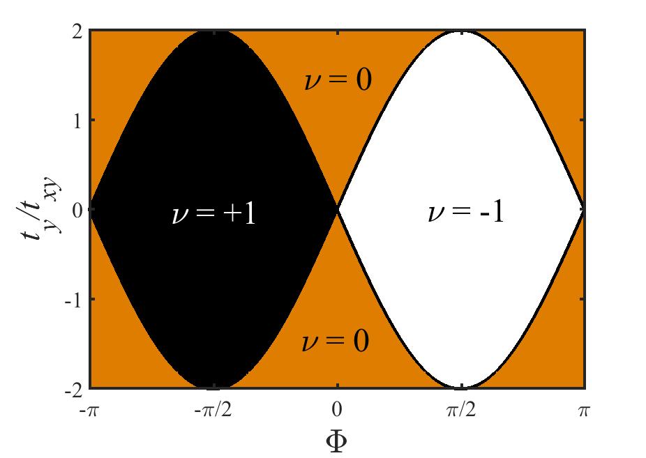
Figure 2: Phase diagram of the system where gap closure occurs. The numbers in the figures denote the topological winding number.

For the spinful model we study, Eqs. (4) and (7) the time-reversal and particle-hole operators take the form $T=i(I_{2}\otimes\sigma_{y})K$, $C=i(\sigma_{y}\otimes\sigma_{x})K$. In this case the square of the operators is $T^{2}=C^{2}=-1$, and $S^{2}=1$, placing these models in the CII symmetry class. One can refine the symmetry characterization further by also considering the reflection operator Chiu13 ; Chiu16 , which sends $k$ to $-k$ without altering the spin. This operator is $R=(I_{2}\otimes\sigma_{x})$, which anti-commutes with $T$, but commutes with $C$. In terms of mirror symmetry class Chiu13 ; Chiu16 the model falls in class $C$, with a topological index of $2\mathbb{Z}$.

For the a chiral symmetric Hamiltonian (Eq. (2)) we apply a unitary transformation Ryu10 , constructed from spinors of spin in the $y$ direction,

$$U=\frac{1}{\sqrt{2}}\begin{pmatrix}1&1\\ i&-i\end{pmatrix},$$ (9)

to our Hamiltonian. This leaves us with the off-diagonal form,

$$\mathcal{H}_{T}=U^{\dagger}\mathcal{H}U=\hskip 56.9055pt$$ (10)

$$=2t_{x}\cos(k)\sigma_{x}+[t_{y}-2t_{xy}\sin(k)]\sigma_{y}=\begin{pmatrix}0&q\\ q^{\dagger}&0\end{pmatrix}.$$

where $q=2t_{x}\cos(k)-i[t_{y}-2t_{xy}\sin(k)]$. The winding number density is given by,

$$w(k)=iq^{-1}(k)\partial_{k}q(k),$$ (11)

from which the winding number can be obtained by integrating across the full Brillouin zone after setting $t_{x}=t_{xy}=1$, resulting in

$$\mathcal{W}=\int_{-\pi}^{\pi}\frac{dk}{2\pi}w(k),$$ (12)

which can be turned into a contour integral around the unit circle via $z=e^{ik}$. If the point $(0,it_{y}/2)$ is within the ellipse defined by $(2t_{x}\cos(k),2t_{xy}\sin(k))$ with $0\leq k<2\pi$, the winding number is minus one. Otherwise it is zero.

We proceed to extend this result to Eq. (4). In this case we have 4-by-4 block-diagonal Hamiltonian,

$$\mathcal{H}(k)=2t_{x}\cos(k)\sigma_{0}\otimes\sigma_{z}-2t_{xy}\sin(k)\sigma_{z}\otimes\sigma_{x}+t_{y}\sigma_{0}\otimes\sigma_{x}$$

$$=\begin{pmatrix}h^{\uparrow}&0\\ 0&h^{\downarrow}\end{pmatrix}$$ (13)

where

$$h^{\uparrow,\downarrow}=\begin{pmatrix}2t_{x}\cos(k)&t_{y}\mp 2t_{xy}\sin(k)\\ t_{y}\mp 2t_{xy}\sin(k)&-2t_{x}\cos(k)\end{pmatrix}$$

After transforming Hamiltonian under $(\sigma_{0}\otimes U)$, where $U$ is given by Eq. (9),

$$\mathcal{H}_{T}(k)=(\sigma_{0}\otimes U)^{\dagger}\;\mathcal{H}(k)\;(\sigma_{0}\otimes U)=\begin{pmatrix}h^{\uparrow}_{T}&0\\ 0&h^{\downarrow}_{T}\end{pmatrix}$$ (14)

where $h^{\uparrow}_{T}=\begin{pmatrix}0&q_{1}\\ q_{1}^{\dagger}&0\end{pmatrix}$ and $h^{\downarrow}_{T}=\begin{pmatrix}0&q_{2}\\ q_{2}^{\dagger}&0\end{pmatrix}$ while

$$q_{1}=2t_{x}\cos(k)-i(t_{y}-2t_{xy}\sin(k))$$

$$q_{2}=2t_{x}\cos(k)-i(t_{y}+2t_{xy}\sin(k)).$$ (15)

Notice that our $4\times 4$ Hamiltonian is simply two independent Creutz models. The overall winding number will be the sum of the winding number of each Creutz model, the two possible values therefore are minus two or zero, depending on whether the point $z=-it_{y}/2$ falls inside or outside the ellipse defined by the Brillouin zone, respectively.

The fundamental group corresponding to topological index of the Hamiltonian of each spin channel is $\mathbb{Z}$. The space of $\mathcal{H}_{T}$ is decomposed into direct sum of subspaces of $h^{\uparrow}$ and $h^{\downarrow}$:

$$\mathcal{H}_{T}=h^{\uparrow}\oplus h^{\downarrow},$$ (16)

hence, the fundamental group representation of topological index can be written as sum of fundamental groups of two subspaces,

$$2\mathbb{Z}=\mathbb{Z}+\mathbb{Z}$$ (17)

which is consistent with symmetry analysis outcome.

IV Středa-Widom formula for quantum spin Hall systems

In the case of the QH effect, a very useful Yilmaz15 ; Hetenyi18 formula was derived by Středa Streda82 via quantum transport equations, and also by Widom Widom82 via thermodynamic Maxwell relations. The generalization to the QSH effect, similar to the Středa approach, was done by Yang and Chang Yang06 . Here we attempt to derive this via Widom’s thermodynamic considerations.

As a starting point, we take the view that a topological insulator consists of two magnets of opposite polarization for each spin. We also invoke a spin-dependent magnetic field, and a corresponding spin-dependent vector potential, ${\bf B}_{\sigma}$ and ${\bf A}_{\sigma}$, respectively. Such a procedure was recently applied by Dyrdal et al. Dyrdal16 to calculate the properties of a two-dimensional electron gas with Rashba spin-orbit coupling. Under the first assumption the spin current can be written as

$${\bf J}_{SH}=c\nabla\times\left[{\bf M}_{\uparrow}-{\bf M}_{\downarrow}\right].$$ (18)

We can derive the electric field from the chemical potential as ${\bf E}=\nabla(\mu/e)$, we can write the spin current as

$${\bf J}_{SH}=(ec){\bf E}\times\frac{\partial}{\partial\mu}\left[{\bf M}_{\uparrow}-{\bf M}_{\downarrow}\right].$$ (19)

We can apply the Maxwell relation and arrive at

$${\bf J}_{SH}={\bf E}\times\left[\frac{\partial(nec)}{\partial{{\bf B}_{\uparrow}}}-\frac{\partial(nec)}{\partial{{\bf B}_{\downarrow}}},\right].$$ (20)

resulting in a QSH conductivity of

$$\sigma_{SH}=ec\left[\frac{\partial n}{\partial{B_{\uparrow}}}-\frac{\partial n}{\partial{B_{\downarrow}}}\right]_{\mu},$$ (21)

where we took the magnetic fields for both spins to be pointing perpendicular to the plane (justifying the neglect of tensor notation). We can rewrite this expression in terms of particle number and magnetic flux as

$$\sigma_{SH}=\left[\frac{\partial\nu}{\partial{\Phi_{\uparrow}}}-\frac{\partial\nu}{\partial{\Phi_{\downarrow}}}\right]_{\mu}.$$ (22)

This expression points to a definite procedure to calculate $\sigma_{SH}$; calculate the Fermi level in the absence of flux, then introduce a spin-dependent flux quantum, and count the number of particles which cross the Fermi level. In our approximate implementation, we use equal and opposite flux for the different spin channels on the $t_{xy}$ bonds. Following Dyrdal et al. Dyrdal16 we neglect the effect of the spin-dependent vector potentials on the Rashba spin-orbit coupling term.

V Results

The gap in the band structure of the shifted Creutz model closes at $k=-\pi/2$ and $\pi/2$ depending on whether $t_{y}=2t_{xy}$ or $t_{y}=-2t_{xy}$. When the boundary conditions are open edge states are found as shown in the shifted Creutz model (Fig. 3). The combination of two shifted Creutz models, one for each spin, restore time reversal invariance with gap closures at $k=\pm\frac{\pi}{2}$. Obviously, this system will also exhibit edge states.

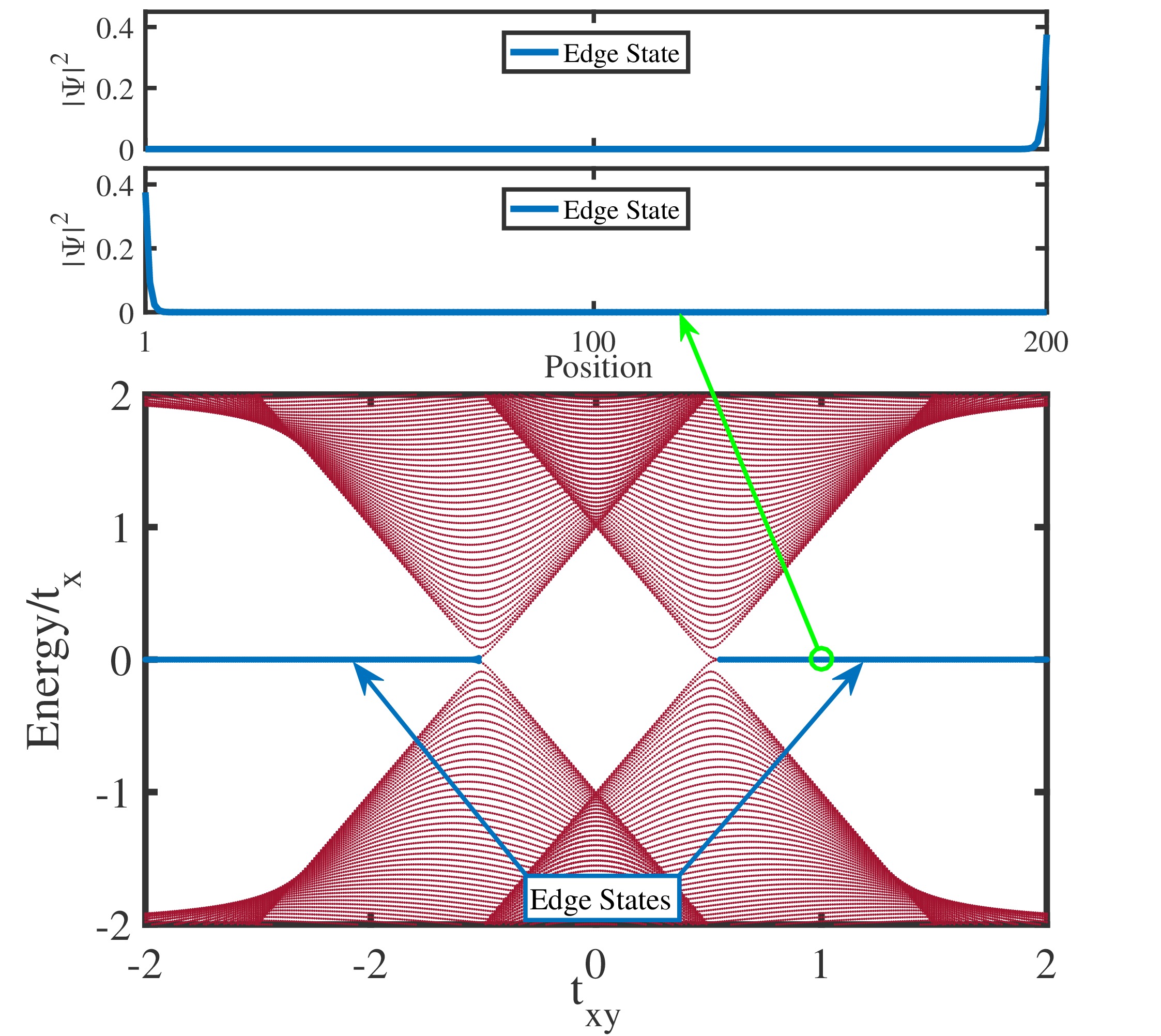
Figure 3: Energy spectrum of the shifted Creutz model with $200$ sites, open boundary conditions as a function of $t_{xy}$. The parameters are $t_{x}=1$ and $t_{y}=1$. The blue lines indicate states which are not present when periodic boundary conditions are applied. The square magnitude of these states are shown in the upper panels. They are localized near the edges of the chain.

Turning on the Rashba coupling term gives rise to a phase diagram shown in Fig. 4 for three cases. The plots are based on a calculation in which $t_{x}=1$, $t_{xy}=0.03,0.18$ and $0.30$. The phase diagram in the $\lambda_{R}/t_{xy}$ vs. $t_{y}/t_{xy}$ is shown for these three cases. The topological phase is the one which includes the origin, outside of this region the phase is trivial. The lines indicate where gap closure occurs. Along the phase boundary the system becomes an ideal conductor with a finite Drude weight. The inset shows the absolute value of the $k$ points at which the gap closure occurs as a function of $t_{y}/t_{xy}$.

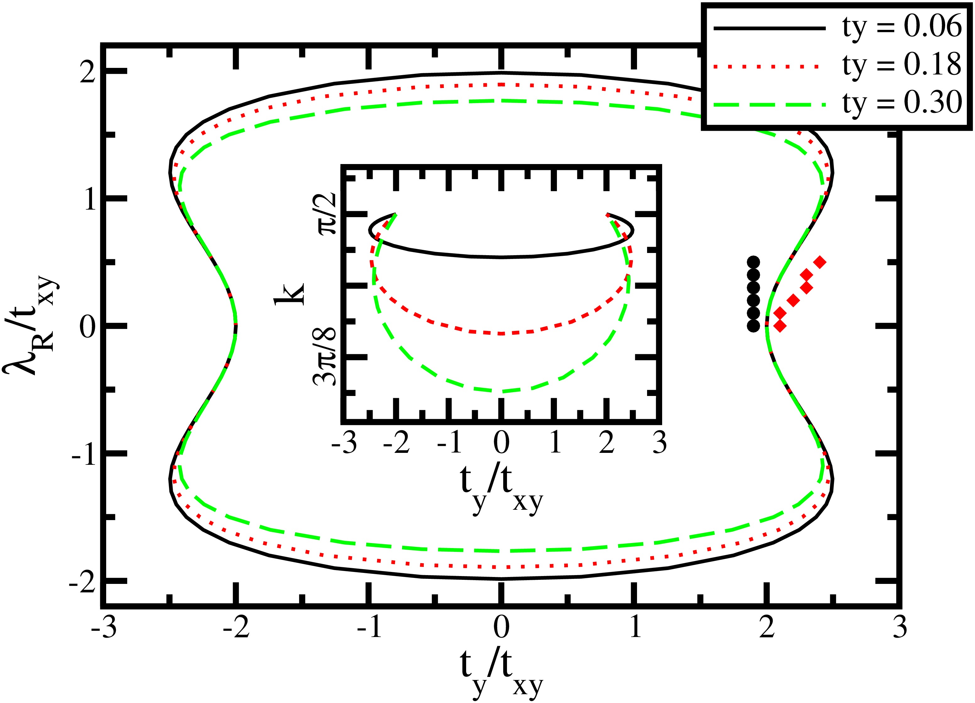
Figure 4: Main figure: phase diagram for systems with $t_{x}=1,t_{xy}=0.06,0.12,0.18$ in the $t_{y}$ vs. $\lambda_{R}$ plane. The inset indicates the $k$ vector at which gap closure occurs as a function of $t_{y}/t_{xy}$. The black filled circles and red filled diamonds on the left side of the phase diagram indicate systems for which we have tested our Středa-Widom formula. For the black filled circles we found a quantized quantum spin Hall response, while we found no response for the red diamonds.

We also studied the quantized transport properties of the models, based on the approximate implementation of the result in Eq. (21). For no Rashba coupling we find that the trivial phase exhibits no $\sigma_{SH}$ response, in other words, upon turning on the spin-dependent flux on the diagonal bonds leads to no change in the number of particles below the Fermi level. In the topological phase, the flux decreases the number of particles under the Fermi level by two. For small values of the Rashba coupling $\lambda_{R}\approx 0.5t_{xy}$ we find the same. In Fig. 4 we indicate the points at which we made calculations (black filled circles and red filled diamonds). At larger values of $\lambda_{R}$ our approximations appear to break down. However, we emphasize that the topological region is adiabatically connected to the $\lambda_{R}=0$ region and is therefore the same quantum phase (also characterized by the $2\mathbb{Z}$ winding number derived above).

VI Conclusion

In conclusion we have assembled a one-dimensional ladder analog of the Kane-Mele model, step by step, first by “shifting” the Creutz model in the Brillouin zone, then introducing spin and spin-orbit coupling. Our model falls in the CII symmetry class. We also derived a formula for the quantum spin Hall response and made an approximate implementation. For small values of the Rashba coupling, where our approximation is expected to be valid, we find a quantized spin Hall response in the topological phase indicating that QSH currents flowing along the legs of the ladder are a unique feature exhibited by our model.

The experimental realization of our model can most likely be done with cold atoms in optical lattices. Standard one-dimensional models Bloch08 already have some history in this setting, but even more complex ones, such as multi-orbital ladder model with topologically non-trivial behavior can be realized Sun12 . There are several interesting routes, for example, it is possible to construct Strinati17 optical lattices with cold atoms in which the atomic states play the role of spatial indices, a technique known as synthetic dimension. A more difficult aspect is the presence of spin-orbit couplings. In two dimensions this was only done recently Grusdt17 , via a combination of microwave driving and lattice shaking. A key development in this experiment is that the different spin-orbit couplings can be varied independently, therefore Kane-Mele like models can be built.

References

- (1) M. Z. Hasan and C. L. Kane, Rev. Mod. Phys. 82 3045 (2010).
- (2) F.D.M. Haldane, Phys. Rev. Lett. 61 2015 (1988).
- (3) C. L. Kane and E. J. Mele, Phys. Rev. Lett. 95 226801 (2005).
- (4) C. L. Kane and E. J. Mele, Phys. Rev. Lett. 95 146802 (2005).
- (5) W. P. Su, J. R. Schrieffer, and A. J. Heeger, Phys. Rev. Lett. (1979).
- (6) M. J. Rice and E. J. Mele, Phys. Rev. Lett. 49 1455 (1982).
- (7) M. Creutz and I. Horváth, Phys. Rev. D 50 2297 (1994).
- (8) M. Creutz, Phys. Rev. Lett. 83 2636 (1999).
- (9) A. Y. Kitaev, Phys-Usp. 44 131 (2001).
- (10) X. Li, E. Zhao, and W. V. Liu Nat. Comm. 4 1523 (2013).
- (11) L. Li, Z. Xu, and S. Chen, Phys. Rev. B 89 085111 (2014).
- (12) R. Wakatsuki, M. Ezawa, Y. Tanaka, N. Nagaosa, Phys. Rev. B 90 014505 (2014).
- (13) T. J. Atherton, C. A. M. Butler, M. C. Taylor, I. R. Hooper, A. P. Hibbins, J. R. Sambles, and H. Mathur, Phys. Rev. B 93 125106 (2016).
- (14) B. Hetényi and M. Yahyavi, J. Phys.: Cond. Mat. 30 10LT01 (2018).
- (15) D. Sticlet, L. Seabra,F. Pollmann, and J. Cayssol, Phys. Rev. B 89 115430 (2014).
- (16) D. Sticlet, B. Dóra, and J. Cayssol, Phys. Rev. B 88 205401(2013).
- (17) O. Viyuela, A. Rivas, and M. A. Martin-Delgado, Phys. Rev. Lett. 112 130401 (2014).
- (18) A. Bermudez, D. Patané, L. Amico, and M. A. Martin-Delgado Phys. Rev. Lett. 102 135702 (2009).
- (19) M. C. Strinati, E. Cornfeld, D. Rossini, S. Barbarino, M. Dalmonte, R. Fazio, E. Sela, and L. Mazza, Phys. Rev. X 7 021033 (2017).
- (20) K. Sun, W. V. Liu, A. Hemmerich, and S. Das Sarma, Nat. Phys. 8 67 (2012).
- (21) A. Altland and M. R. Zirnbauer Phys. Rev. B 55 1142 (2997).
- (22) A. P. Schnyder, S. Ryu, A. Furusaki, and A. W. W. Ludwig Phys. Rev. B 78 195125 (2008).
- (23) C.-K. Chiu, H. Yao, and S. Ryu, Phys. Rev. B 88 075142 (2013).
- (24) C.-K. Chiu, J. C. Y. Teo, and A. P. Schnyder, Rev. Mod. Phys. 88 035005 (2016).
- (25) S. Ryu, A. P. Schnyder, A. Furusaki, and A. W. W. Ludwig New J. Phys. 12 065010 (2010).
- (26) R. Jackiw and C. Rebbi, Phys. Rev. D 13 3398 (1976).
- (27) R. Resta, Phys. Rev. Lett. 80 1800 (1998).
- (28) R. Resta and S. Sorella, Phys. Rev. Lett. 82 370 (1999).
- (29) I. Bloch, Nature 453 1016 (2008).
- (30) F. Yilmaz, F. Nur Ünal, M. Ö. Oktel, Phys. Rev. A 91 063628 (2015).
- (31) P. Středa, J. Phys. C 15 L717 (1982).
- (32) A. Widom, Phys. Lett. A 474 90 (1982).
- (33) M.-F. Yang and M.-C. Chang, Phys. Rev. B 73 073304 (2006).
- (34) A. Dyrdal, V. K. Dugaev, and J. Barnaś, Phys. Rev. B 94 205302 (2016).
- (35) I. Bloch, Nature 453 1016 (2008).
- (36) F. Grusdt, T. Li, I. Bloch, and E. Demler, Phys. Rev. A 95 063615 (2017).