Puzzling Lyman-alpha line profiles in green pea galaxies

Abstract

Context. The Lyman-alpha (Ly$\alpha$) line of hydrogen is of prime importance for detecting galaxies at high redshift. For a correct data interpretation, numerical radiative transfer models are necessary due to Ly$\alpha$ resonant scattering off neutral hydrogen atoms.

Aims. Recent observations have discovered an escape of ionizing Lyman-continuum radiation from a population of compact, actively star-forming galaxies at redshift $z\sim 0.2-0.3$, also known as “green peas”. For the potential similarities with high-redshift galaxies and impact on the reionization of the universe, we study the green pea Ly$\alpha$ spectra, which are mostly double-peaked, unlike in any other galaxy sample. If the double peaks are a result of radiative transfer, they can be a useful source of information on the green pea interstellar medium and ionizing radiation escape.

Methods. We select a sample of twelve archival green peas and we apply numerical radiative transfer models to reproduce the observed Ly$\alpha$ spectral profiles, using the geometry of expanding, homogeneous spherical shells. We use ancillary optical and ultraviolet data to constrain the model parameters, and we evaluate the match between the models and the observed Ly$\alpha$ spectra. As a second step, we allow all the fitting parameters to be free, and examine the agreement between the interstellar medium parameters derived from the models and those from ancillary data.

Results. The peculiar green pea double-peaked Ly$\alpha$ line profiles are not correctly reproduced by the constrained shell models. Conversely, unconstrained models fit the spectra, but parameters derived from the best-fitting models are not in agreement with the ancillary data. In particular: 1) the best-fit systemic redshifts are larger by 10 – 250 km s^-1 than those derived from optical emission lines; 2) the double-peaked Ly$\alpha$ profiles are best reproduced with low-velocity ($\lesssim\!\!150$ km s^-1) outflows that contradict the observed ultraviolet absorption lines of low-ionization-state elements with characteristic velocities as large as 300 km s^-1; and 3) the models need to consider intrinsic Ly$\alpha$ profiles that are on average three times broader than the observed Balmer lines.

Conclusions. Differences between the modelled and observed velocities are larger for targets with prominent Ly$\alpha$ blue peaks. The blue peak position and flux appear to be connected to low column densities of neutral hydrogen, leading to Ly$\alpha$ and Lyman-continuum escape. This is at odds with the kinematic origin of the blue peak in the homogeneous shell models. Additional modelling is needed to explore alternative geometries such as clumpy media and non-recombination Ly$\alpha$ sources to further constrain the role and significance of the Ly$\alpha$ double peaks.

1 Introduction

Green peas (GPs) are a local population of compact ($<3$ kpc), low-mass ($10^{8-10}M_{\odot}$) galaxies with strong optical emission lines (Cardamone et al., 2009; Izotov et al., 2011) found at redshifts $z<0.5$. Their popular name was coined by the citizen science Galaxy Zoo project (Lintott et al., 2008), where the targets appear unresolved in the Sloan Digital Sky Survey (SDSS) images and have green colours due to the strong [O iii]$\,\lambda 5007$ nebular emission line, with equivalent widths as large as $\sim\!1500$ Å. Izotov et al. (2011) have shown that green peas form a subset of luminous compact galaxies that are present in the SDSS over a larger redshift range, $0.02\!\lesssim\!z\!\lesssim\!0.65$. Their compactness, low masses, sub-solar metallicities in the range 12 + log(O/H) $\sim$ 7.5 – 8.5, and H$\alpha$ equivalent widths exceeding hundreds of Å (Izotov et al., 2011) make green peas similar to high-redshift Lyman-break galaxies (LBGs) and Lyman-alpha emitters (LAEs).

Green peas have recently drawn attention due to the ionizing Lyman continuum (LyC) radiation escape. The detected LyC that manages to leak into the intergalactic space proves that starburst galaxies could have played a role in the cosmic reionization. Such detections have been rare to date: while six out of the six targeted green peas leak $6-46$ % of their LyC (Izotov et al., 2016a, b, 2018), only four additional low-$z$ LyC leakers have been found over the past two decades, and their escape fractions are low, $f_{\mathrm{esc}}$(LyC) = 1 – 4% (Bergvall et al., 2006; Leitet et al., 2013; Borthakur et al., 2014; Leitherer et al., 2016; Puschnig et al., 2017). At high redshift, the situation is even more challenging; numerous LyC leaking candidates have been refuted as lower-redshift interlopers (Siana et al., 2015), and stringent upper limits have been set on the escape fractions for $z\!\sim\!1\!-\!2$ galaxies using the Galaxy Evolution Explorer (GALEX) and Hubble Space Telescope (HST) imaging catalogues (Rutkowski et al., 2016, 2017). Only three convincing spectroscopic LyC detections (de Barros et al., 2016; Vanzella et al., 2016; Shapley et al., 2016; Vanzella et al., 2018) and one imaging detection (Bian et al., 2017) have recently been achieved at $z\!\sim\!2-4,$ reaching, however, large escape fractions, $f_{\mathrm{esc}}$(LyC) $>50$%, for each of these galaxies.

The Lyman continuum escape from green peas had been suspected due to their high star-formation rates, compactness, and high [O iii]$\,\lambda 5007$/[O ii]$\,\lambda 3727$ flux ratios, unusual for local galaxies, which could be signatures of density-bounded H ii regions (Jaskot & Oey, 2013; Nakajima et al., 2013; Nakajima & Ouchi, 2014; Stasińska et al., 2015). Furthermore, most of the green peas were known to be strong Lyman-alpha (Ly$\alpha$) emitters with unusual Lyman-alpha (Ly$\alpha$) line profiles consisting of narrow, double-peaked emission lines, and weak ultraviolet (UV) absorption lines of low-ionization-state metals (Jaskot & Oey, 2014; Henry et al., 2015; Verhamme et al., 2015). These UV properties are consistent with a low H i content, leading to the ionizing radiation escape, as was theoretically demonstrated by Verhamme et al. (2015), and observationally confirmed by Verhamme et al. (2017) and Chisholm et al. (2017).

The Ly$\alpha$ line of hydrogen (1215.67 Å) is one of the primary tools for detecting high-$z$ galaxies (e.g. Ouchi et al., 2009; Sobral et al., 2015; Matthee et al., 2015; Zitrin et al., 2015; Oesch et al., 2016; Bagley et al., 2017). It also is a powerful tool to study conditions in the interstellar medium (ISM), both at low and high redshift (e.g. Hayes et al., 2013, 2014; Verhamme et al., 2015; Guaita et al., 2017). Ly$\alpha$ resonantly scatters off neutral hydrogen, which results in strong radiative transfer effects both in real and frequency space. The escape of Ly$\alpha$ from galaxies is a complex, multi-parameter problem: Ly$\alpha$ photons trapped by scattering are more susceptible to dust absorption. On the other hand, outflows, low dust contents, and low H i column densities help their escape (e.g. Kunth et al., 1998; Shapley et al., 2003; Atek et al., 2008; Verhamme et al., 2008; Scarlata et al., 2009; Wofford et al., 2013; Hayes et al., 2014; Hayes, 2015; Henry et al., 2015; Rivera-Thorsen et al., 2015). Building on the early analytical works (Adams, 1972; Neufeld, 1990), numerical Ly$\alpha$ radiation transfer models were needed to demonstrate the effects of the ISM conditions on the Ly$\alpha$ spectral profiles. Monte Carlo codes computing the Ly$\alpha$ transfer in simplified plane-parallel or spherical geometries proved to be useful for this task at a relatively low computational cost (Ahn et al., 2001; Verhamme et al., 2006; Dijkstra et al., 2006; Barnes & Haehnelt, 2010; Dijkstra & Kramer, 2012; Laursen et al., 2013; Duval et al., 2014; Zheng & Wallace, 2014; Behrens et al., 2014; Verhamme et al., 2015; Dijkstra et al., 2016; Gronke et al., 2015; Gronke & Dijkstra, 2016; Gronke et al., 2016). Application of the models to real galaxies has successfully reproduced most of the observed Ly$\alpha$ profile features (e.g. Verhamme et al., 2008; Dessauges-Zavadsky et al., 2010; Noterdaeme et al., 2012; Krogager et al., 2013; Hashimoto et al., 2015; Martin et al., 2015; Yang et al., 2016, 2017a).

The similarity of green peas to high-redshift LBGs and LAEs (Cardamone et al., 2009; Izotov et al., 2011; Jaskot & Oey, 2013; Nakajima & Ouchi, 2014; Schaerer et al., 2016) make them important low-$z$ laboratories for studying the LyC and Ly$\alpha$ escape mechanisms, essential for understanding the formation and evolution of galaxies across the cosmic history. Various aspects of the Ly$\alpha$ emission in green peas were addressed by Jaskot & Oey (2014), Henry et al. (2015), Yang et al. (2016), Yang et al. (2017a), Verhamme et al. (2015), and Verhamme et al. (2017). Radiative transfer models were used by Yang et al. (2016, 2017a) to interpret Ly$\alpha$ profiles of fifty-five GPs. Their modelling generally achieved acceptable fits between the single-shell homogeneous models and the GPs. In this paper, we reinterpret the archival HST Cosmic Origins Spectrograph (COS) observations of Ly$\alpha$ from twelve green peas studied by Yang et al. (2016). Using an independent radiative transfer code (Verhamme et al., 2006), we extend this study by including observational ISM constraints. If we apply no constraints, we reproduce the Yang et al. (2016) results and successfully fit the observed Ly$\alpha$ profiles. However, we show that the ISM parameters characterizing the best-fitting models are in disagreement with those measured from independent UV and optical data. If we impose the observational constraints in the fitting process, the homogeneous shell models do not provide good fits to the data. We evaluate the mismatches and discuss the validity of the models for these peculiar spectra.

We structure the paper as follows. We describe the data in Sect. 2 and the Ly$\alpha$ radiative transfer models in Sect. 3. We present the model fitting results both with and without the application of observational constraints in Sect. 4. We discuss the differences between modelled and observed ISM parameters, their correlations, and model limitations in Sect. 5.

2 Data sample

Table 1: Green pea sample.

ID	RA	DEC	$z$
GP 0303	03 03 21.41	$-$07 59 23.2	0.16489
GP 0816	08 15 52.00	$+$21 56 23.6	0.14095
GP 0911	09 11 13.34	$+$18 31 08.2	0.26224
GP 0926	09 26 00.44	$+$44 27 36.5	0.18070
GP 1054	10 53 30.80	$+$52 37 52.9	0.25265
GP 1133	11 33 03.80	$+$65 13 41.4	0.24140
GP 1137	11 37 22.14	$+$35 24 26.7	0.19440
GP 1219	12 19 03.98	$+$15 26 08.5	0.19561
GP 1244	12 44 23.37	$+$02 15 40.4	0.23942
GP 1249	12 48 34.63	$+$12 34 02.9	0.26340
GP 1424	14 24 05.72	$+$42 16 46.3	0.18480
GP 1458	14 57 35.13	$+$22 32 01.8	0.14859

2.1 Observations and archival data

HST Ly$\alpha$ data:

We use archival far-ultraviolet (FUV) spectra of twelve green pea galaxies at redshift $z\!\!\sim\!\!0.2$ (Table 1), observed with the Hubble Space Telescope (HST) under programmes GO 12928 (PI A. Henry), GO 13293 (PI A. Jaskot), and GO 11727 (PI T. Heckman). The Ly$\alpha$ spectra were obtained with the $2.5\arcsec$ Primary Science Aperture (PSA) of the Cosmic Origins Spectrograph (COS) onboard the HST, with the use of the medium resolution grism G160M. We use the standard pipeline-reduced data obtained through the Mikulski Archive for Space Telescopes (MAST). Details of the observations and various target properties were included in Henry et al. (2015), Jaskot & Oey (2014), and Heckman et al. (2011). Additional information on the target GP 0926 from the HST imaging and ground-based spectroscopy are available in Basu-Zych et al. (2009), Gonçalves et al. (2010), Hayes et al. (2013), Hayes et al. (2014), Rivera-Thorsen et al. (2015), and Herenz et al. (2016).

The COS spectral resolution depends on the size of the source: the resolving power varies between $R\!=\!16\,000$ ($<20$ km s^-1) for a point source and $R\!=\!1500$ ($200$ km s^-1) for a uniformly filled aperture (see the COS handbook). The COS acquisition near-UV images reveal that the green pea diameters are $\lesssim 1\arcsec$ (Henry et al., 2015). We assume that the Ly$\alpha$ emission extent is typically a factor of two to four larger than the stellar continuum extent, based on the analysis of the GP cross-dispersion sizes in the two-dimensional COS spectra (Yang et al., 2017b). A similar result was achieved by deep HST Advanced Camera for Surveys (ACS) imaging of nearby star-forming galaxies (Hayes et al., 2013, 2014). We estimate the COS resolution for GPs to be $\sim\!100$ km s^-1, under the assumption that the Ly$\alpha$ emission distribution is peaked, as is the usual case in the known star-forming galaxies (Hayes et al., 2014). This is consistent with the Ly$\alpha$ spectra appearance: sharp peaks and troughs on the one hand, and the lack of more detailed Ly$\alpha$ sub-features on the other. We have rebinned the COS spectra to a sampling of 25 km s^-1.

Ancillary HST UV measurements:

Aside from Ly$\alpha$, the COS far-UV (FUV) spectra include a series of absorption lines of low-ionization-state (LIS) metals, such as Si ii. Due to the low ionization potential of these species, the lines provide valuable information on geometry and kinematics of the H i gas, where Ly$\alpha$ propagates. The LIS lines of our sample were analysed in Jaskot & Oey (2014), Henry et al. (2015), and Yang et al. (2016), and we adopt here their kinematic parameters to describe the H i medium for Ly$\alpha$ modelling (Sect. 4.1).

Ancillary optical SDSS data:

We use the optical Sloan Digital Sky Survey (SDSS) spectra to measure the emission-line redshifts (Henry et al., 2015) and to estimate parameters of the intrinsic Ly$\alpha$ line, that is, the line as it would appear before radiation transfer. If both Ly$\alpha$ and the Balmer lines are produced by the same recombination process, their respective luminosities are tied together through scaling laws, set by atomic physics. While Ly$\alpha$ undergoes a resonant radiative transfer in neutral hydrogen, Balmer lines travel through the medium unaltered by H i, and are only attenuated by dust. The observed H$\alpha$ and/or H$\beta$ line profiles corrected for the instrumental dispersion thus carry information about the intrinsic Ly$\alpha$ line width. Their flux corrected for dust absorption then provides an estimate of the total produced Ly$\alpha$ before it undergoes the radiative transfer. The SDSS spectra have spectral resolution $R\!\sim\!2000$ (150 km s^-1), and were obtained with circular $3\arcsec$ optical fibres, similar to the $2.5\arcsec$ COS aperture. The GPs are compact, unresolved in the SDSS, and therefore the difference between the COS and SDSS apertures is not significant (but see Sects. 3 and 4 where we discuss the possible impacts). With the medium SDSS spectral resolution, the information about the intrinsic Ly$\alpha$ is limited to the total flux and basic kinematics, of which we make full use in this paper. All of our data and models have been corrected for the instrumental dispersion. We describe the application of the constraints in more detail in Sect. 4.1.

2.2 Description of the sample: Ly$\alpha$ line profiles

Table 2: Ly$\alpha$ spectral shape parameters.

ID	$v_{B}$	$v_{R}$	Blue/Red	trough
	[km s-1]	[km s-1]	EW ratio	[km s-1]
	(1)	(2)	(3)	(4)
GP 0303	$-300\pm 60$	$150\pm 40$	0.06	$-110\pm 50$
GP 0816	$-210\pm 40$	$140\pm 50$	0.36	$-20\pm 40$
GP 0911	$-290\pm 50$	$80\pm 40$	0.17	$-60\pm 40$
GP 0926	$-160\pm 100$	$220\pm 120$	0.14	$-40\pm 40$
GP 1054	$-220\pm 100$	$200\pm 40$	0.11	$70\pm 80$
GP 1133	$-90\pm 40$	$230\pm 60$	0.51	$70\pm 60$
GP 1137	$-250\pm 100$	$170\pm 50$	0.12	$-20\pm 40$
GP 1219	$-80\pm 40$	$170\pm 50$	0.38	$20\pm 40$
GP 1244	$-240\pm 40$	$250\pm 40$	0.33	$-10\pm 40$
GP 1249	—	$80\pm 40$	0.00	—
GP 1424	$-150\pm 60$	$220\pm 40$	0.67	$70\pm 40$
GP 1458	$-360\pm 60$	$390\pm 100$	0.40	$40\pm 60$

We describe here the main features of the observed Ly$\alpha$ line profiles, and derive the first implications for radiative transfer, independent of any model geometry.

Double-peaked emission lines:

As already noted by Henry et al. (2015) and Yang et al. (2016), all of the twelve green peas show Ly$\alpha$ in net emission, which is unusual for other local star-forming galaxy samples of similar size (Wofford et al., 2013; Rivera-Thorsen et al., 2015). The net Ly$\alpha$ emission is only prevalent in galaxy samples selected by their high FUV luminosity, the Lyman-break analogues (LBAs, see Heckman et al., 2011; Alexandroff et al., 2015). Strangely, none of the GP Ly$\alpha$ spectra have a P-Cygni profile with a redshifted emission and a blueshifted absorption, which is often considered as the typical Ly$\alpha$ line signature, mainly in high $z$. The Ly$\alpha$ line is double-peaked in eleven of the twelve targets of our GP sample, and similar statistics are present in other GP samples, such as those of Verhamme et al. (2017) and Yang et al. (2017a), which is truly unusual for any other galaxy sample. In high redshift, multiple-peak Ly$\alpha$ profiles have drawn observers’ attention only recently, after their discovery in low-$z$ galaxies, such as in Heckman et al. (2011), Martin et al. (2015), and Alexandroff et al. (2015). The Ly$\alpha$ line identification in distant LAEs was traditionally done by its asymmetric single peak. Kulas et al. (2012) and Trainor et al. (2015) estimated the incidence of multiple peaks to be $\sim\!30$% among UV-selected star-forming galaxies $z=2-3$ showing Ly$\alpha$ emission. The actual number can be higher, due to the blue peak attenuation by the inter-galactic medium (IGM) (Laursen et al., 2011; Dijkstra, 2014). Also, the typical spectral resolution in high-$z$ observations is lower than that of the HST/COS, and therefore some of the spectral profiles can in reality be double peaks, such as those with non-zero flux blueward of the systemic redshift (Erb et al., 2014),

The relative equivalent width ($EW$) of the blue peaks varies across our sample, and it represents 5 – 65% of the red peak $EW$ (Table 2). To measure the blue and red $EW$s, we separated the Ly$\alpha$ profile into two parts, divided by the central trough between the peaks. This differs from the definition previously used in the literature (Heckman et al., 2011; Erb et al., 2014; Henry et al., 2015), where separation between the blue and red parts of the spectra was defined by the systemic redshift. Our definition reflects the sufficient data resolution and the need to characterize the individual peaks, independently of the redshift (see Discussion).

We infer, from the systematically stronger red peak, that the GP Ly$\alpha$ is transferred in outflowing media. This is consistent with the measurements of UV absorption lines that originate from low-ionization state (LIS) metal species, which are blueshifted with respect to the systemic redshift, and thus indicate outflows. The red Ly$\alpha$ dominance is model independent and has been illustrated analytically and numerically in various geometries such as slabs (Neufeld, 1990), spherical shells (e.g. Verhamme et al., 2006; Dijkstra et al., 2006), and in radiative transfer coupled to full hydrodynamic simulations (e.g. Verhamme et al., 2012). The double-peaked profiles may have various origins, such as Ly$\alpha$ transfer in low-velocity media, in clumpy media or other, less studied, geometries. We will discuss this question in Sect. 5.

Ly$\alpha$ profile symmetries:

We have (re-)measured the positions of the red and blue Ly$\alpha$ peaks, and of the troughs that separate them (Table 2). Without any modelling at this stage, we determined the local flux maxima and minima. Uncertainties resulting from the peak shape and flux variations were included in the error bars, together with the wavelength calibration uncertainties. In the cases where the Ly$\alpha$ peak or trough had a multi-component character, or where the peak top had a peculiar shape with a varying flux (such as flat-top blue peaks with flux variations in GP 1054 or GP 1137), we computed the mean position of the components, and included their variance in the uncertainty. This definition, which was the best choice for the comparison with models, may differ from that applied in Henry et al. (2015) or Yang et al. (2016), and we find differences in some of the measurements. Nevertheless, the measurements are consistent with the independent papers within the stated error bars.

We provide the peak and trough positions in the form of velocity offsets, measured from the systemic redshift that was derived from the SDSS emission lines (Table 1). We considered the combined wavelength calibration error of the SDSS and the HST/COS to be 40 km s^-1 (Henry et al., 2015). We find that the central Ly$\alpha$ trough is redshifted with respect to the systemic redshift in five targets of the sample (GP 1054, GP 1133, GP 1219, GP 1424, and GP 1457), that is usually those with strong blue peaks (Table 2). In at least two of them (GP 1133 and GP 1424) the shift cannot be explained by measurement errors, which include the systematic uncertainty on the wavelength calibration, noise on the spectral line profile, and additional features in the trough. These two targets also have the largest relative flux of the blue peak. The redshifted Ly$\alpha$ troughs are surprising and were not expected in galaxies with H i outflows: due to the Doppler shift in the outflows, the largest Ly$\alpha$ optical depth should be shifted from zero to negative velocities (Verhamme et al., 2006). In a reversed configuration, an inflow, the trough would be placed in positive velocities. However, the blue peak should dominate the flux in that case, which is not what we observe in the GPs. The inflow scenario therefore seems improbable.

We illustrate the peak and trough positions in Fig. 1, where the targets have been sorted by their blue peak offset, measured either with respect to the systemic redshift (Fig. 1a) or to the central trough position (Fig. 1b). The red and blue peak positions are not symmetric. Ordering of the targets by their blue peak offset did not produce any alignment in the red peak offset. We will see in Sect. 5.5 that the peaks are not equally broad either, and we will discuss the implications for the radiative transfer models.

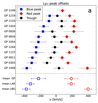
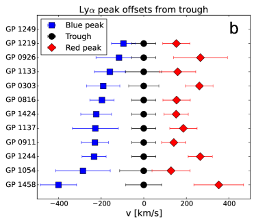
Figure 1: Asymmetry of the blue and red Ly$\alpha$ peaks in the GP sample, measured from a) the systemic redshift, and b) the central trough. Panel (a) also includes the mean positions of the blue and red peaks for this GP sample, and for LAE and LBG samples drawn from the literature (Hashimoto et al., 2015). The GPs are similar to the LAEs in the red peak positions, but have a smaller mean blue offset.

Low column density of neutral hydrogen:

The GP Ly$\alpha$ profiles are unusually narrow, with a small separation between their peaks ($400\pm 100$ km s^-1). We show in Fig. 1a that this separation is smaller than in typical high-$z$ LAEs ($510\pm 60$ km s^-1) and LBGs ($770\pm 60$ km s^-1), drawn from the Hashimoto et al. (2015) sample. While the major difference between LBG and LAE double-peaked profiles is in the red peak position ($400\pm 40$ km s^-1 in LBGs, $190\pm 40$ km s^-1 in LAEs), it is the blue peak that drives the difference between the GPs and the high-$z$ samples ($-370\pm 50$ km s^-1 in LBGs, $-320\pm 50$ km s^-1 in LAEs, and $-210\pm 90$ km s^-1 in GPs). The observed small separations show that Ly$\alpha$ is able to escape close to the systemic redshift and that the effects of radiative transfer are relatively weak, irrespective of the model geometry (Verhamme et al., 2015). Several ISM parameters can contribute to achieve this condition: low $N_{\mathrm{HI}}$, large H i velocities, or a clumpy medium with low-density inter-clump gas. Observations have proved that the Ly$\alpha$ peak offsets are small in galaxies with escaping Lyman continuum (Izotov et al., 2016a, b, 2018) and that the double-peak separation correlates with the LyC escape fraction (Verhamme et al., 2017). The LyC escape requires a low H i column density along the line of sight, $N_{\mathrm{HI}}$ $\lesssim 10^{18}$ cm^-2 if the ISM is homogeneous. The Ly$\alpha$ spectra of our GP sample are similar to those of the LyC leakers, therefore there is a high probability that the GPs studied here have analogously low H i column densities (no direct confirmation exists, no LyC observations are available for the present sample).

A large opacity in the Ly$\alpha$ line core produces a trough separating the red and blue peaks. However, the trough does not reach the zero flux level in approximately half of our sample (GP 0816, GP 0911, GP 1133, GP 1219, and GP 1424), confirming that the opacity (and thus $N_{\mathrm{HI}}$) is surprisingly low. Yang et al. (2016) found a correlation between the residual flux in the trough and the Ly$\alpha$ escape fraction, which suggests that the non-zero flux is not an artificial effect caused by an insufficient spectral resolution. Sub-features can be seen in the central trough of GP 1133: two minima separated by 80 km s^-1. This could indicate that the line core is either partially refilled with emission, or that the blue minimum corresponds to the deuterium absorption, as discussed in Dijkstra et al. (2006) and Verhamme et al. (2006).

Another confirmation of the low $N_{\mathrm{HI}}$ in the GPs comes from the absence of underlying broad Ly$\alpha$ absorption, analogously to $z\!\sim\!0.3$ LyC leakers (Verhamme et al., 2017). Star-forming galaxies with observed Ly$\alpha$ emission lines commonly show an underlying absorption trough, with wings visible on a much wider wavelength scale than the emission spectrum (see e.g. Wofford et al., 2013; Rivera-Thorsen et al., 2015; Duval et al., 2016; Schaerer & Verhamme, 2008; Dessauges-Zavadsky et al., 2010; Quider et al., 2010). From the modelling point of view, as Ly$\alpha$ resonantly scatters off H i, the absorption part of the spectrum is the result of the photon removal from the line of sight, while emission is produced by photons scattered out of resonance. The absorption trough becomes deeper and broader with the increasing column density of the foreground H i, and with aperture losses (Verhamme et al., 2006, 2017). We have done a careful inspection of the continuum in all twelve GPs, and found no signs of absorption, except for a shallow trough in GP 1458 and possibly in GP 0303. The absence points to generally low H i column densities in GPs, likely similar to those in LyC leakers of Izotov et al. (2016a, b, 2018).

Comparison between Ly$\alpha$ and H$\beta$ profiles:

If produced by pure recombination, the intrinsic Ly$\alpha$ line profile (before radiative transfer) should share the kinematic characteristics of the Balmer lines, and be their scaled version. Radiative transfer effects transform the Ly$\alpha$ profile by removing photons most strongly from the line centre, redistributing them to the wings, or destroying them by absorption. The resultant profile is broadened, attenuated, and with shifted peaks. Figures 2 and 4 show a direct comparison between the observed Ly$\alpha$ profile and H$\beta$ scaled by the Case B factor of 23.5 (Dopita & Sutherland, 2003). The figures also present the results of model fitting (Sect. 4), while here we focus on the comparison of the observational profiles. We used H$\beta$ instead of H$\alpha$, which partially blends with the [N ii] lines and would impede studying the line wings. We present the data with subtracted continuum, which was fit by a first order polynomial in the vicinity of H$\beta$ and Ly$\alpha$. We corrected both H$\beta$ and Ly$\alpha$ fluxes for the Milky Way (MW) extinction (Schlafly & Finkbeiner, 2011) using the Cardelli et al. (1989) extinction law. The MW extinction values were obtained from the NASA Extragalactic Database (NED) and were listed in Henry et al. (2015) and Yang et al. (2016). The H$\beta$ flux was additionally corrected for internal extinction using the SDSS H$\alpha$ and H$\beta$ fluxes with the assumption of their intrinsic ratio of 2.86 (Dopita & Sutherland, 2003), and using the Cardelli et al. (1989) extinction law. The corrected H$\beta$ flux was then used to approximate the intrinsic Ly$\alpha$ line flux. No correction for internal extinction was applied to Ly$\alpha$, as it is not attenuated in the same way as the optically thin lines, and its radiative transfer includes effects of both gas and dust.

The observed Ly$\alpha$ blue wings are as broad as those of the scaled H$\beta$ line in most of the sample. For two targets, GP 0303 and GP 0911, such a similarity is also seen in the red wing. This is unusual, and signifies that the Ly$\alpha$ profile has not been much broadened by radiative transfer. Remarkably, Martin et al. (2015) draw a similar conclusion for a sample of low-$z$ ultraluminous infrared galaxies (ULIRGs). We note that SDSS resolution is worse than that of COS. However, we have tested that degrading the COS spectra to the SDSS resolution does not change our conclusion about the wings.

Table 3: Measured and model-fit parameters.

	Observed ISM parameters (HST/COS, SDSS)				Shell model results from unconstrained fitting
ID	$v_{\mathrm{LIS}}$	FWHM(H$\beta$)	$\tau_{\mathrm{d,obs}}$	EW0(Ly$\alpha$)obs	$\Delta z$	$v_{\mathrm{exp}}$	$b$	$\log N_{\mathrm{HI}}$	$\tau_{\mathrm{d}}$	FWHM0(Ly$\alpha$)	EW0(Ly$\alpha$)
	[km s-1]	[km s-1]	FUV	[Å]	[km s-1]	[km s-1]	[km s-1]	[cm-2]	FUV	[km s-1]	[Å]
(1)	(2)	(3)	(4)	(5)	(6)	(7)	(8)	(9)	(10)	(11)	(12)
GP 0303	$-200^{+80}_{-80}$	160	0	150${}^{+50}_{-50}$	$60^{+60}_{-0}$	$150^{+50}_{-0}$	$20^{+30}_{-10}$	$19.0^{+0.3}_{-1.2}$	$1^{+2}_{-1}$	$500^{+100}_{-120}$	$15^{+5}_{-5}$
GP 0816	$-300^{+100}_{-100}$	130	0.4${}^{+0.2}_{-0.2}$	200${}^{+100}_{-100}$	$10^{+50}_{-0}$	$20^{+30}_{-0}$	$20^{+0}_{-10}$	$19.0^{+0.3}_{-1}$	$0.2^{+0.8}_{-0.2}$	$400^{+100}_{-0}$	$75^{+25}_{-25}$
GP 0911	$-250^{+50}_{-50}$	220	2.6${}^{+1.4}_{-1.4}$	140${}^{+110}_{-110}$	$30^{+0}_{-70}$	$100^{+50}_{-0}$	$20^{+20}_{-0}$	$18.5^{+0.5}_{-0.7}$	$1.5^{+1.5}_{-0.5}$	$500^{+0}_{-100}$	$50^{+25}_{-0}$
GP 0926	$-280^{+100}_{-100}$	170	1.5${}^{+0.8}_{-0.8}$	120${}^{+70}_{-70}$	$140^{+5}_{-50}$	$150^{+50}_{-0}$	$20^{+0}_{-10}$	$18.5^{+0.5}_{-0.7}$	$1^{+1}_{-1}$	$550^{+50}_{-50}$	$40^{+10}_{-10}$
GP 1054	$-180^{+80}_{-80}$	230	1.3${}^{0.7}_{-0.7}$	140${}^{+50}_{-50}$	$150^{+40}_{-40}$	$150^{+0}_{-0}$	$40^{+40}_{-0}$	$19.3^{+0}_{-1.5}$	$1^{+2}_{-1}$	$150^{+250}_{-50}$	$20^{+10}_{-10}$
GP 1133	—	160	0.2${}^{+0.1}_{-0.1}$	100${}^{+50}_{-50}$	$160^{+50}_{-0}$	$50^{+0}_{-30}$	$10^{+0}_{-0}$	$18.5^{+0.5}_{-0}$	$0.5^{+2.5}_{-0.5}$	$600^{+0}_{-100}$	$35^{+5}_{-5}$
GP 1137	$-150^{+50}_{-50}$	210	1.0${}^{+0.6}_{-0.6}$	200${}^{+100}_{-100}$	$100^{+0}_{-50}$	$150^{+100}_{-0}$	$40^{+120}_{-20}$	$18.7^{+0.3}_{-2.7}$	$1^{+0.5}_{-1}$	$550^{+60}_{-300}$	$40^{+10}_{-10}$
GP 1219	—	160	0.03${}^{+0.02}_{-0.02}$	200${}^{+100}_{-100}$	$115^{+50}_{-0}$	$50^{+50}_{-0}$	$20^{+0}_{-10}$	$18.0^{+0.5}_{-2}$	$0.2^{+0.8}_{-0.2}$	$600^{+0}_{-100}$	$125^{+0}_{-25}$
GP 1244	$-90^{+50}_{-50}$	170	1.1${}^{+0.6}_{-0.6}$	400${}^{+300}_{-300}$	$150^{+0}_{-100}$	$150^{+0}_{-100}$	$40^{+0}_{+0}$	$18.5^{+1.1}_{-0.5}$	$0.5^{+1.6}_{-0.3}$	$1000^{+0}_{-300}$	$75^{+25}_{-25}$
GP 1249	$-180^{+50}_{-50}$	160	0.7${}^{+0.2}_{-0.2}$	200${}^{+100}_{-100}$	$80^{+50}_{-50}$	$250^{+0}_{-50}$	$10^{+10}_{-0}$	$16.0^{+2}_{-0}$	$2^{+2}_{-1}$	$400^{+0}_{-0}$	$75^{+5}_{-0}$
GP 1424	$-240^{+50}_{-50}$	210	0.7${}^{+0.4}_{-0.4}$	200${}^{+100}_{-100}$	$120^{+50}_{-0}$	$50^{+50}_{-30}$	$20^{+20}_{-10}$	$19.0^{+0.3}_{-1.5}$	$0.2^{+0.8}_{-0.2}$	$700^{+30}_{-100}$	$75^{+40}_{-25}$
GP 1458	$-30^{+70}_{-70}$	130	0.4${}^{+0.3}_{-0.3}$	400${}^{+300}_{-300}$	$55^{+0}_{-45}$	$20^{+0}_{-0}$	$40^{+0}_{-20}$	$20.2^{+0.3}_{-0}$	$1^{+0.5}_{-0.5}$	$400^{+100}_{-250}$	$100^{+200}_{-50}$

3 Radiative transfer models

3.1 Code and model grid

We use an enhanced version of the MCLya 3D Monte Carlo code of Verhamme et al. (2006), which computes radiative transfer of the Ly$\alpha$ line and the adjacent UV continuum for an arbitrary three-dimensional (3D) geometry and velocity field. We here assume the geometry of an expanding, homogeneous, spherical shell composed of neutral hydrogen and dust, uniformly mixed. A starburst region, which is the source of the Ly$\alpha$ and UV continuum photons, is placed at the centre of the sphere filled with ionized gas and surrounded by the neutral shell. The photons are collected after their propagation through the neutral shell in all directions. The expanding geometry was motivated by the H i outflows, which we detect in the studied galaxies (Henry et al., 2015) and which additionally seem to be ubiquitous at both low- and high-redshifts (e.g. Shapley et al., 2003; Wofford et al., 2013; Rivera-Thorsen et al., 2015; Chisholm et al., 2015). The spherical configuration was motivated by the observation of superbubbles in star-forming galaxies, as described by for example Tenorio-Tagle et al. (1999) and Mas-Hesse et al. (2003). The MCLya models have previously been successfully applied to reproduce the Ly$\alpha$ spectra of low- and high-$z$ galaxies (Verhamme et al., 2008; Schaerer & Verhamme, 2008; Dessauges-Zavadsky et al., 2010; Vanzella et al., 2010; Lidman et al., 2012; Leitherer et al., 2013; Hashimoto et al., 2015; Duval et al., 2016; Patrício et al., 2016).

The modelled shell is characterized by four parameters: the radial expansion velocity $v_{\mathrm{exp}}$, the H i column density $N_{\mathrm{HI}}$, the optical depth $\tau_{\mathrm{d}}$ of dust at wavelengths in the vicinity of Ly$\alpha$, and the H i  Doppler parameter $b$ that describes the internal shell kinematics including thermal and turbulent velocities. Photons from the source have an initial frequency distribution, and the path and the frequency change through the shell are followed for each of them. A grid of $>\!6000$ synthetic models was constructed by varying the shell parameters and running the full MCLya simulation for each parameter set (Schaerer et al., 2011). The resulting spectra were then post-processed to account for the intrinsic line profile, and were further smeared to match the observed spectral resolution estimated from the Ly$\alpha$ source extent.

We define the initial, intrinsic Ly$\alpha$ profile assuming a flat stellar UV continuum and a Ly$\alpha$ emission line, which can either be a Gaussian, a double-Gaussian, or another function, such as the observed Balmer line profile. If we assume a Gaussian profile, the model adjustment has seven free parameters. Four parameters describe the H i shell: $v_{\mathrm{exp}}$, $N_{\mathrm{HI}}$, $b$, $\tau_{\mathrm{d}}$; and three parameters describe the Gaussian line: the line width $FWHM_{0}$(Ly$\alpha$), the equivalent width $EW_{0}$(Ly$\alpha$), and the line centre, that is, the redshift $z$. Each of the fitting parameters regulates a different measurable characteristics of the resultant Ly$\alpha$ profile (Verhamme et al., 2006; Gronke et al., 2015). The profiles are most sensitive to $v_{\mathrm{exp}}$ and $N_{\mathrm{HI}}$, both of which determine the offset of the resultant Ly$\alpha$ emission peak from the restframe position, while $v_{\mathrm{exp}}$ also determines the $EW$ of the Ly$\alpha$ blue peak. The intrinsic Ly$\alpha$ equivalent width $EW_{0}$(Ly$\alpha$) and the dust optical depth $\tau_{\mathrm{d}}$ regulate the Ly$\alpha$ flux scaling, and a large dust content usually results in a prominent absorption trough in the blue part of the profile if the medium is expanding. Large $N_{\mathrm{HI}}$ and $\tau_{\mathrm{d}}$ give rise to broad Ly$\alpha$ absorption profiles. The role of $b$ is less straightforward to describe and is usually degenerate with other parameters.

We use an automated line profile fitting tool (Schaerer et al., 2011), which explores the entire grid or its defined part. The fitting parameters can either be constrained to definite values or to intervals of values. The fitting procedure then searches for the minimum $\chi^{2}$ and computes the $\chi^{2}$ maps. We here define intervals for the fitting parameters that either correspond to the observational uncertainties (Sect. 4.1) or to the entire grid extent (Sect. 4.3). We keep twenty best-fitting models for each fitting run and each target to have a better control of the fitting parameter stability. We describe their use for the different fitting approaches in the respective sections.

3.2 Constraining the free parameters

Depending on the availability of ancillary data, several of the fitting parameters can be constrained. In the present sample, we were able constrain up to five parameters using the optical SDSS and UV HST/COS data (Tables 1 and 3):

1. Redshift $z$ (Table 1): derived from Gaussian fits of $\sim\!20$ SDSS emission lines with a precision better than $10$ km s^-1 (Henry et al., 2015). Applied to the Ly$\alpha$ line, the redshift uncertainty is dominated by the wavelength calibration errors, $\sim\!40$ km s^-1 (Sect. 2.1).

2. Expansion speed $v_{\mathrm{exp}}$ of the shell: measured from the UV absorption line offsets of low-ionization species, which are commonly observed blueshifted, that is, outflowing. We report the characteristic LIS line velocities $v_{\mathrm{LIS}}$ in Table 3. The velocities measured by Henry et al. (2015) show variations between different transitions, which can be attributed to either noise or different amounts of emission filling (Scarlata & Panagia, 2015). We list here their mean and consider the full range of velocities reported in that paper in order to give our Ly$\alpha$ models the best chance to match the observations. We have measured the missing velocities.

3. Optical depth of dust absorption in the FUV, $\tau_{\mathrm{d}}$: estimated from the SDSS Balmer line ratios by extrapolation to the FUV domain using extinction laws from the literature. An inherent uncertainty associated with this estimate arises from the uncertainty in the extinction law – the commonly used laws give similar predictions in the optical range, but dramatically vary in the FUV. We report in Table 3 the mean value and variance of $\tau_{\mathrm{d}}$ derived from the extinction laws of Cardelli et al. (1989), Calzetti et al. (1994), and Prevot et al. (1984).

4. Full width at half maximum of the intrinsic Ly$\alpha$ line, $FWHM_{0}$(Ly$\alpha$), is assumed to be identical to that of H$\beta$ if both lines are formed by the same recombination mechanism. We fitted the SDSS H$\beta$ line profiles with two-component Gaussian functions, narrow and broad. We list the width of the dominating narrow component, $FWHM$(H$\beta$), in Table 3, and the broad component width and flux contribution in Table 4. The line widths have been corrected for the instrumental dispersion. We assume an uncertainty of 100 km s^-1 in the $FWHM$(H$\beta$).

5. Intrinsic Ly$\alpha$ equivalent width, $EW_{0}$(Ly$\alpha$): estimated from the observed H$\beta$ flux and the observed FUV continuum, assuming that both lines were formed by recombination. Pure Case B recombination at $T=10\,000$ K and $n_{\mathrm{e}}=10^{-2}$ cm^-3 predicts the Ly$\alpha$/H$\beta$ flux ratio of 23.5 (Dopita & Sutherland, 2003). Both the measured line and continuum fluxes were corrected for dust attenuation, and therefore the uncertainties in the extinction law induce uncertainties in $EW_{0}$(Ly$\alpha$). In addition, the differences between the nebular and continuum attenuation (Calzetti, 1997; Price et al., 2014), the possible need for aperture corrections accounting for the differences between SDSS and COS, and the possible deviations in the temperature gave rise to the range of $EW_{0}$(Ly$\alpha$) for each target reported in Table 3.

No constraints are available for the H i column $N_{\mathrm{HI}}$, and the Doppler parameter $b$. To constrain $b$, high-resolution absorption lines would be necessary, resolving the individual H i clouds. Therefore, $b$ and $N_{\mathrm{HI}}$ are considered as free fitting parameters, ranging across the entire grid of models: $10$ km s^-1 $\leq b\leq 160$ km s^-1, and $10^{16}$ cm^-2 $\leq$ $N_{\mathrm{HI}}$ $\leq 10^{23}$ cm^-2.

For those parameters that require a comparison between the SDSS and the HST/COS data, we need to consider the differences between the spectrographs: 1) the aperture size, and 2) the spectral resolution. The different aperture sizes, 2.5″ in the HST/COS versus 3″ in the SDSS, potentially affect the measured fluxes, and can therefore impact the $EW_{0}$(Ly$\alpha$) derived from H$\beta$. However, the near-UV HST/COS acquisition images (Henry et al., 2015) show that the GPs are extremely compact, smaller than the aperture size. The GP optical images are unresolved in the SDSS, but we expect a similar morphology and extent as in the near-UV (based on Hayes et al., 2013, 2014). Nevertheless, to account for the possibility that the true optical emission is much larger than the acquisition image and that the aperture size matters for the derivation of the intrinsic Ly$\alpha$, we considered both situations, with and without the aperture correction to derive $EW_{0}$(Ly$\alpha$) from $EW$(H$\beta$). Both cases were reflected in the $EW_{0}$(Ly$\alpha$) intervals that we list in Table 3. No correction was applied to the observed Ly$\alpha$ emission due to its unpredictable nature. It is possible that a part of Ly$\alpha$ is transferred outside the COS aperture, which we will further discuss in the following sections. Concerning the spectral resolution, it plays a role in the derivation of the intrinsic Ly$\alpha$ profile from H$\beta$. The SDSS resolution is worse (150 km s^-1) than the HST/COS resolution for Ly$\alpha$ ($\sim\!100$ km s^-1, Sect. 2). With the given SDSS resolution, our H$\beta$ application is restricted to the instrument-corrected $FWHM$, with no other details about the line profile. To account for the COS resolution in the fitting process, we adjust the Ly$\alpha$ grid model spectra correspondingly. We show in the following sections that the observed Ly$\alpha$ spectra would be better reproduced with an input line broader than the SDSS profile, which cannot be explained by the difference in spectral resolution. On the other hand, other inconsistencies between models and data could potentially be better understood with the aid of high-resolution spectroscopy.

4 Ly$\alpha$ line profile modelling

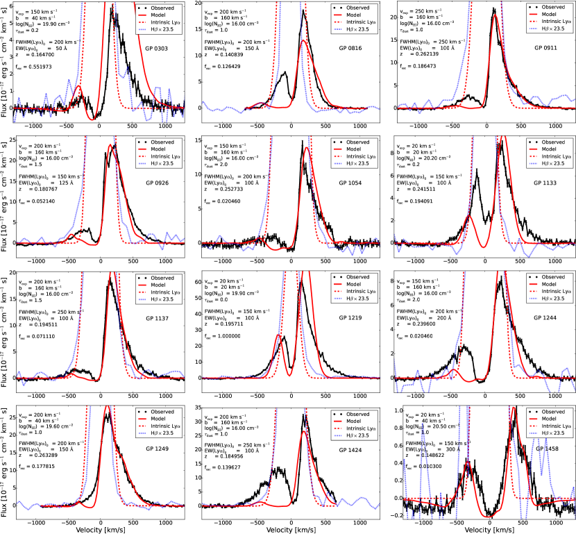
Figure 2: Best-fitting Ly$\alpha$ models with applied constraints from ancillary observational data (Sect. 4.1). COS data and their errorbars are shown in black, the best-fitting model with the solid red line, the modelled intrinsic single-Gaussian Ly$\alpha$ profile with the dashed red line, and the observed SDSS H$\beta$ scaled by Case B factor 23.5 with the dotted blue line. Parameters of the best-fitting model are shown in each panel.

We have carried out Ly$\alpha$ profile modelling with the use of the model grid described in Sect. 3 and with the application of observational constraints. As we will see in Sections 4.1 and 4.2, the constrained models do not reproduce all the features of the observed profiles, and we will therefore explore their failure and will relax all the constraints in Sect. 4.3.

4.1 Ly$\alpha$ profile fitting with constraints

We have described the derivation of the constraining parameters in Sect. 3. Assuming a Gaussian profile of the intrinsic Ly$\alpha$ line, with the $FWHM$ equal to the dominant, narrow component of H$\beta$, five of the seven fitting parameters can be constrained. For fitting purposes, the parameters were assigned the intervals listed in columns 2 – 5 of Table 3, which reflect the observed values and their uncertainties. Redshifts and line widths were considered with conservative errors of 50 km s^-1 and 100 km s^-1, respectively, to account for the COS wavelength calibration and for the SDSS line decomposition into Gaussians. The $v_{\mathrm{exp}}$ velocity remains a free fitting parameter in two targets, GP 1133 and GP 1219, where no UV LIS lines have been detected. The Ly$\beta$ line is available, but its proper modelling would be necessary to disentangle the stellar and ISM contributions, therefore we have not used it. Before the Ly$\alpha$ fitting, we convolved the synthetic grid spectra with a Gaussian function, which simulated the finite spectral resolution, 100 km s^-1 (Sect. 2). We carried out a series of tests to check how the spectral resolution would affect the fits. Model spectra convolved with too broad or too narrow profiles were not compatible with the observed features of the Ly$\alpha$ profile (not sharp enough peaks and troughs, or too detailed substructure, respectively). A good match was achieved at $\sim\!100\pm 30$ km s^-1, which is consistent with the COS estimation derived from the target morphology. We note that this convolution was missing in the work of Yang et al. (2016), which may explain some of the differences between their results and this work.

We have run the fitting tool on the model sub-grid defined by the constraints, keeping twenty models with the lowest $\chi^{2}$ for each target. The twenty models served as a visual check of the model matching. We plot the data and the lowest-$\chi^{2}$ model for each galaxy in Fig. 2. We overplot the theoretical intrinsic Ly$\alpha$ line, derived from the best-fitting model, and the observed SDSS H$\beta$ line scaled by the Case B factor of 23.5. To enable the comparison, all observational and modelling data were converted to velocity units, and the respective continuum was subtracted from each line. The intrinsic Ly$\alpha$ model was convolved with a Gaussian profile corresponding to the SDSS resolution for a direct comparison with the SDSS data. The best-fitting model parameters are listed in each panel. Any differences between the model parameters and the ancillary data parameters, or between the intrinsic Ly$\alpha$ and H$\beta$ profiles, are due to the observational uncertainties and the discreteness of the model grid.

We immediately notice large discrepancies between the fits and the data. The models dramatically fail in reproducing the blue peak for almost every target, in both flux and position. The match for the red peaks is better and can be considered satisfactory in approximately half of the sample, while the peak positions and widths disagree with the observations in the remaining targets. Furthermore, the central trough positions of the double-peaked models are offset with respect to the observed troughs. The homogeneous shell models regulate the relative blue peak flux by $v_{\mathrm{exp}}$, while the trough position is the location of the maximum optical depth, dependent on $z$ and $v_{\mathrm{exp}}$, and cannot be forced by any other combination of the remaining parameters. With $z$ and $v_{\mathrm{exp}}$ fixed by the observational constraints, the fitting algorithm can only attempt to reproduce the peak positions by varying $N_{\mathrm{HI}}$, which was a free parameter here, but cannot produce the correct peak flux ratios and trough positions. In the logic of the homogeneous models, the ancillary data did not provide the correct $z$ and $v_{\mathrm{exp}}$ in the studied GPs. The failure to correctly fit troughs in GP 1133 and GP 1219, where $v_{\mathrm{exp}}$ was a free parameter, indicates that $v_{\mathrm{exp}}$ alone is not sufficient to solve the problem.

4.2 Ly$\alpha$ source modelled by a double Gaussian

Table 4: Parameters of double-Gaussian fits of the SDSS H$\beta$ line.

ID	$FWHM_{\mathrm{broad}}$ [km s-1]	$f_{\mathrm{broad}}$/$f_{\mathrm{narrow}}$
	(1)	(2)
GP 0303	400 $\pm$ 100	0.20 $\pm$ 0.05
GP 0816	350 $\pm$ 100	0.
GP 0911	450 $\pm$ 100	0.5 $\pm$ 0.1
GP 0926	500 $\pm$ 100	0.50 $\pm$ 0.03
GP 1054	500 $\pm$ 100	0.33 $\pm$ 0.07
GP 1133	450 $\pm$ 100	0.1 $\pm$ 0.1
GP 1137	500 $\pm$ 100	0.30 $\pm$ 0.05
GP 1219	500 $\pm$ 100	0.33 $\pm$ 0.05
GP 1244	400 $\pm$ 100	0.25 $\pm$ 0.05
GP 1249	350 $\pm$ 100	0.2 $\pm$ 0.1
GP 1424	500 $\pm$ 100	0.20 $\pm$ 0.03
GP 1458	400 $\pm$ 100	0.10 $\pm$ 0.03

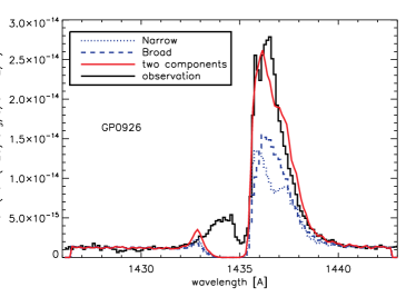
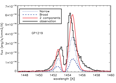
Figure 3: Constrained fits using double-Gaussian intrinsic Ly$\alpha$ profiles, with a realistic proportion of broad and narrow components, derived from SDSS H$\beta$ spectra. Targets with the largest broad component contribution are shown.

We searched for the reasons for the bad correspondence between the observed and modelled Ly$\alpha$ profiles resulting from model fitting with constraints. We first considered a better description of the intrinsic Ly$\alpha$ profiles with several kinematic systems. This effort was motivated by Amorín et al. (2012), who showed complex kinematic structures in GP H$\alpha$ profiles observed with a high-resolution ($R\!>\!10\,000$) echelle spectrograph. None of their targets have been observed in Ly$\alpha$, therefore no direct proof of the effect of multiple kinematic components on the resultant Ly$\alpha$ is available. At the SDSS resolution, no strong secondary line components are detected in our sample, but broad H$\alpha$ and H$\beta$ wings are consistently seen (Henry et al., 2015).

We therefore fitted the SDSS H$\alpha$ and H$\beta$ lines with double-Gaussian profiles, narrow and broad. At the SDSS resolution, the double-Gaussian fits produce degenerate results, we therefore used both H$\alpha$ and H$\beta$ to minimize the degeneracy. The kinematic parameters were tied between the lines, while they were independent between the broad and narrow components. The Gaussian amplitudes were free parameters in each line, and we computed the mean between H$\alpha$ and H$\beta$ for each component. We found that the broad and narrow components have redshift differences $\pm 30$ km s^-1, that is, they are the same within the uncertainties. Unlike in dusty galaxies, the red wing is not extinguished, and the broad component is symmetric about the systemic redshift. We obtain broad-to-narrow flux ratios in the range $0\!-\!0.5$. We included the narrow component $FWHM$ in Table 3, and we list the broad component $FWHM$ and the flux ratios of the broad and narrow components in Table 4. The flux ratios represent the mean between H$\alpha$ and H$\beta$. We assume the uncertainty of the broad component $FWHM$ to be $\sim\!100$ km s^-1, based on multiple trials of the double-Gaussian fitting. All $FWHM$s have been corrected for instrumental dispersion.

We assumed that both narrow and broad H$\beta$ components were produced by recombination, and we used the double-Gaussian profiles as input characterizing the intrinsic Ly$\alpha$ profiles for Ly$\alpha$ model fitting. We present the fitting results for two targets that are among those with the largest broad component flux fraction (GP 0926, GP 1219) in Fig. 3. The resulting fits have not significantly improved over those with single Gaussians. Even though the blue peaks have become slightly more pronounced, the Ly$\alpha$ profiles are not well reproduced and the problems encountered in Sect. 4.1 persist.

4.3 Unconstrained fitting

4.3.1 Good fits, discrepant parameters

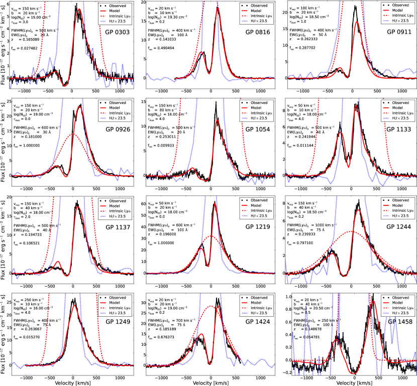
Figure 4: Best-fitting Ly$\alpha$ models, obtained by unconstrained fitting. COS data and their errorbars are shown with the black line, best-fitting model with the solid red line, intrinsic Ly$\alpha$ profile with the dashed red line, and the observed SDSS H$\beta$ scaled by Case B factor 23.5 with the dotted blue line. Derived best-fit parameters of the shell are shown in each panel.

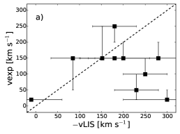
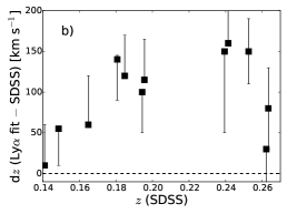
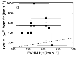
Figure 5: Comparison between parameters derived from the unconstrained Ly$\alpha$ fitting, and their observed counterparts. a) outflow velocity; b) redshift; c) $FWHM_{0}$(Ly$\alpha$). The dashed lines show the expected identity between the parameters. The points and errorbars correspond to those listed in Table 3.

To understand which parameters play a role in producing the unsatisfactory results of the constrained model fitting, we finally relaxed all the constraints. We ran the fitting process across the entire grid of $>\!6000$ MCLya shell models (with four varying shell parameters $v_{\mathrm{exp}}$, $b$, $N_{\mathrm{HI}}$, and $\tau_{\mathrm{d}}$), and we ignored the constraints from the ancillary data. In addition, the parameters of the Ly$\alpha$ source, that is, $EW_{0}$(Ly$\alpha$), $FWHM_{0}$(Ly$\alpha$), and $z$, were also let free. A good match between the best-fitting modelled and observed spectra has been found by the automatic fitting procedure for all of the twelve targets, unlike in Yang et al. (2016), where fitting of GP 1133, GP 1219 and GP 1424 failed.

We present the lowest $\chi^{2}$ model for each galaxy in Fig. 4. To assess how the model parameters differ from the observations, we considered twenty lowest-$\chi^{2}$ models for each target. A visual check revealed that for the given grid resolution, the twenty models encompassed spectra that were still in reasonable agreement with the observations: they matched the positions and amplitudes of the Ly$\alpha$ peaks and troughs, and matched the line wings. A larger number of fits was inappropriate due to the deteriorating fit quality, and we did not opt for a narrower set in order to allow for possibly large intervals in all the fitting parameters, while searching for overlaps with the observed ones. The visual check was complementary to the $\chi^{2}$ parameter computation. This simple method allowed an assessment of the parameter range without a complex fit quality analysis, unnecessary for the problem in hand. To characterize the fitting parameter distribution in each target, we computed their median and the $10^{\mathrm{th}}$ and $90^{\mathrm{th}}$ quantiles in the set of twenty best fits, and used them in Table 3, columns 6 – 12 (the uncertainties here correspond to the quantiles). The quantiles are convenient for the discrete character of the grid and our choice discards only the extremes in each given set.

Figure 4 shows that the homogeneous shell models are able to reproduce the GP Ly$\alpha$ spectra, as in Yang et al. (2016). However, a comparison between the observed and modelled ISM parameters reveals significant disagreement (Table 3). We have identified three major discrepancies, which we describe below and illustrate in Fig. 5:

1. The only way to produce double-peaked Ly$\alpha$ profiles in the shell models is by assuming a static or low-velocity ($\lesssim\!\!150$ km s^-1) H i medium (see Neufeld, 1990; Verhamme et al., 2006; Dijkstra et al., 2006). Therefore, except for the single-peak target GP 1249, all the best fits of our sample have $v_{\mathrm{exp}}$ $\leq$ 150 km s^-1. Spectra with the strongest blue peaks (GP 0816, GP 1133, GP 1219, GP 1424, and GP 1458) required even lower velocities, $v_{\mathrm{exp}}$ $\leq$ 50 km s^-1. In contrast, the observed LIS velocities $v_{\mathrm{LIS}}$ are significantly larger in at least one third of the sample (Fig. 5a). No convincing LIS line detection was possible in GP 1133 and GP 1219, but their high-ionization gas velocities from Si iii and Si iv are between $-300$ and $-400$ km s^-1, and we also find Ly$\beta$ components at similar velocities, inconsistent with the fitted $v_{\mathrm{exp}}$ $\sim 50$ km s^-1. We list the measured LIS velocities with a negative sign in Table 3 (the lines are blueshifted), while we provide a positive $v_{\mathrm{exp}}$, which is defined as the expansion velocity of the shell.

2. Systemic redshifts derived from the Ly$\alpha$ models are larger than those from the SDSS emission lines in every target of the sample. With the exception of three targets, the redshift discrepancy $\Delta z$ is larger than the conservative wavelength calibration uncertainty of 40 km s^-1, and reaches values as high as $\sim\!\!160$ km s^-1 (Fig. 5b). The targets with redshifted Ly$\alpha$ troughs (e.g. GP 1133, GP 1424) described in Sect. 2.2 do not stand out and are part of the trend. The best-fitting model redshifts are driven by the requirement that the central trough should lie at the position of the largest optical depth, close to $-$$v_{\mathrm{exp}}$.

3. Large intrinsic Ly$\alpha$ line widths, $FWHM_{0}$(Ly$\alpha$), were chosen by the best-fitting models to match the shape of the blue Ly$\alpha$ peaks, and the broad blue and red wings. These compensate for the lack of profile broadening in low-$N_{\mathrm{HI}}$ models, determined by the observed small separation of Ly$\alpha$ peaks. The typical best-fit $FWHM_{0}$(Ly$\alpha$) $\sim$ 500 km s^-1 (Fig. 5c) are much larger than the measured SDSS $FWHM$(H$\beta$) $\sim$ 200 km s^-1, and are similar to or larger than the broad component of H$\beta$. However, we cannot conclude from here that the narrow component was attenuated and only the broad one was transmitted. The modelled intrinsic Ly$\alpha$ lines have larger fluxes than the broad components of Balmer lines scaled by the Case B factors. Therefore, we need to interpret this discrepancy as another model failure, not a physical effect.

The remaining free fitting parameters, $b$, $N_{\mathrm{HI}}$, $\tau_{\mathrm{d}}$ and $EW_{0}$(Ly$\alpha$), either have no directly observable counterparts or their comparison to observed values is less straightforward. No measurable counterpart was available for $b$ and $N_{\mathrm{HI}}$. The Doppler parameter $b$ is the least robust fitting parameter (see also Gronke et al., 2015), therefore its large spread in some of the targets is unsurprising. On the contrary, $N_{\mathrm{HI}}$ is among the most robust parameters due to its strong impact on the Ly$\alpha$ peak shift (Verhamme et al., 2006; Gronke et al., 2015). The $N_{\mathrm{HI}}$ that we here derive from the shell models is generally low ($\lesssim 10^{19}\mathrm{\,cm}^{-2}$) compared to typical star-forming galaxies. The modelled FUV attenuation due to dust, $\tau_{\mathrm{d}},$ has a large scatter for each target. This is most probably caused by the low $N_{\mathrm{HI}}$. The role of dust in low-$N_{\mathrm{HI}}$ environments is reduced due to a relatively small number of scattering events and therefore models with a small and large dust content thus give similar results. Nevertheless, given the large uncertainties in both the modelled and observed $\tau_{\mathrm{d}}$ (due to the low $N_{\mathrm{HI}}$ and the uncertainty in the FUV attenuation law), we cannot properly judge the consistency between the observations and the models: we can only state that the results are consistent within the large error bars. Finally, the best-fitting model $EW_{0}$(Ly$\alpha$) is usually lower than that derived from H$\beta$ observations in the studied sample, or is at the lower edge of the interval of possible $EW_{0}$(Ly$\alpha$) values (Table 3). This may indicate that a part of Ly$\alpha$ has been transferred outside the COS aperture, which is consistent with the result obtained from a comparison of the COS and GALEX observations for two GPs (Henry et al., 2015), and from the Ly$\alpha$ HST imaging for GP 0926 (Hayes et al., 2014). It can also indicate a preference for extinction curves with a low total to selective extinction ratio, typical of low-metallicity galaxies and also found in GP-like galaxies of Izotov et al. (2016a, b).

4.3.2 Fit parameter discrepancies are tied to spectral shape

We have tested whether any correlations exist between the fitting parameters or their discrepancies. The first conclusion is that both $v_{\mathrm{exp}}$ and $z$ need to be free parameters in order to reproduce the GP Ly$\alpha$ peaks and troughs, but nothing can be concluded about the correlation between the discrepancies $\Delta z$ and $\Delta v$. Secondly, a hint of correlation was found between the redshift discrepancy $\Delta z$ and the ratio of the intrinsic Ly$\alpha$ and H$\beta$ widths, $FWHM_{0}$(Ly$\alpha$)/$FWHM$(H$\beta$). Larger samples are needed to confirm or refute the correlations.

A natural question is how the difficulties in Ly$\alpha$ fitting are linked to the double-peak character of the line profile, common in the GPs. We devote Fig. 6 to studying several best-fit and observational parameters as a function of the Ly$\alpha$ blue peak flux fraction, expressed as $EW$(Ly$\alpha$)_Blue/$EW$(Ly$\alpha$)_Red. The blue and red peak fluxes were measured as separated by the central trough (and not by the systemic redshift) to better characterize flux in each peak, described in Sect. 2.2. We find that the difference between fitted and measured gas velocities, $v_{\mathrm{exp}}$$-$—$v_{\mathrm{LIS}}$—, generally increases with the increasing blue peak strength (Fig. 6a). With the exception of two points that have high $EW$(Ly$\alpha$)_Blue/$EW$(Ly$\alpha$)_Red$\sim 0.4$ and $v_{\mathrm{exp}}$$-$—$v_{\mathrm{LIS}}$—$\sim 0$, all the other studied galaxies show an anti-correlation between the velocity difference and the blue peak flux fraction (Spearman coefficient $-0.91$ and P-value 0.002). The colour-scale coding of the plot helps clarify that the two outliers have low LIS velocities $\left(<\!100{\textrm{\,km\,s${}^{-1}$}}\right)$. Thanks to them, there is a fortuitous agreement between the modelled and observed values, due to the fact that low velocities are the only way to produce strong blue peaks in the shell models. The colour scale of Fig. 6a also helps to visualize that the double peaks appear in GPs across a large range of LIS velocities. If the GP Ly$\alpha$ blue peaks were due to low gas velocities, we would expect a correlation between the LIS velocities and the observed $EW$(Ly$\alpha$)_Blue/$EW$(Ly$\alpha$)_Red – which we cannot confirm in our data. The blue peaks may thus not be linked to static environments, or alternatively may be formed in static environments not probed by the LIS lines.

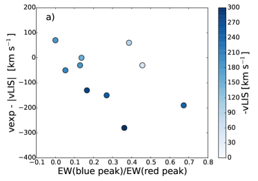
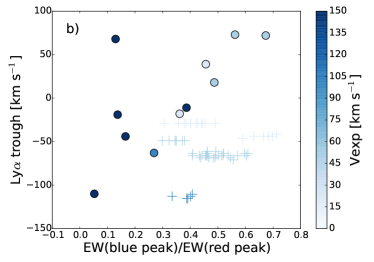
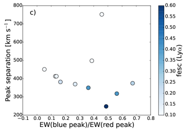
Figure 6: Relations between the Ly$\alpha$ blue and red peak $EW$ ratio, and several observed and best-fit parameters. Circles represent the observed GPs, crosses represent shell models. Details can be found in Sect. 4.3.2.

Figure 6b is devoted to the Ly$\alpha$ trough position, which we described earlier in this paper to be inconsistent with the measured LIS velocities. We observe that as the blue peak grows stronger, the trough shifts from large negative offsets towards the systemic redshift and then to positive offsets. The peculiar shift to positive velocities, unexpected from the modelling, is just a continuation of the overall trend. We also see a trend between the trough position and $v_{\mathrm{exp}}$ (colour scale in the plot): the trough position is most negative for largest $v_{\mathrm{exp}}$ ($>\!100$km s^-1), and positive mostly for low $v_{\mathrm{exp}}$. A correlation between the trough position and both $v_{\mathrm{exp}}$ and relative blue peak $EW$ is indeed expected in the models where the blue peak originates from radiative transfer in low-velocity or static environments: the optical depth is maximum at approximately $-$$v_{\mathrm{exp}}$, therefore the trough offset from the systemic velocity becomes larger with increasing $v_{\mathrm{exp}}$. The blue peak becomes weaker with increasing $v_{\mathrm{exp}}$. However, the models (cross symbols) are not co-spatial with the observed data in Fig. 6b. The model troughs are shifted further to negative velocities and can never reach positive velocities. This illustrates why an adjustment of the systemic redshift is needed to fit the observed profiles.

Finally, Fig. 6c shows the Ly$\alpha$ double-peak separation as a function of the blue-to-red $EW$ ratio and the observed $f_{\mathrm{esc}}$(Ly$\alpha$). Even though purely observational, this plot elucidates the reasons for the incompatibility between the models and GP data. The diagram shows that the stronger the blue peak, the smaller the peak separation in most cases, and the larger the observed $f_{\mathrm{esc}}$(Ly$\alpha$) (colour scale in the same plot). The two outliers with peak separations of $\sim\!500$ km s^-1 and $\sim\!800$ km s^-1 are the same ones as in Fig. 6a, with nearly static kinematics that favour the blue peak formation. The remaining nine GPs do not seem to have blue peaks related to the outflow kinematics but rather to the low H i column density for the following reasons: 1) Ly$\alpha$ double-peak separation is a good tracer of the H i column density (Verhamme et al., 2015, 2017). As we find the smallest Ly$\alpha$ separation in GPs with the largest blue peak flux contribution (Fig. 6c), the probability of the LyC escape increases with the increasing blue peak flux. 2) LyC escape from the GP-like galaxies has been shown to correlate with $f_{\mathrm{esc}}$(Ly$\alpha$) (Verhamme et al., 2017). In our sample, GPs with a large blue peak tend to have a larger Ly$\alpha$ escape fraction (colour scale in Fig. 6c). The anti-correlation between the $EW$(Ly$\alpha$)_Blue/$EW$(Ly$\alpha$)_Red ratio and $f_{\mathrm{esc}}$(Ly$\alpha$) has the Spearman coefficient of 0.85 and p-value of 0.003 if the two outliers with static LIS gas are left out. In addition, we see an anti-correlation between the peak separation and $f_{\mathrm{esc}}$(Ly$\alpha$), with the Spearman coefficient of 0.94 and p-value $10^{-4}.$ Therefore, if the blue peak is not produced in static gas, it is related to the Ly$\alpha$ and potentially the LyC escape. In complementarity to previous GP studies (Henry et al., 2015; Yang et al., 2016, 2017a) we therefore show here that not only the blue peak position but also its relative flux seems to carry information about the transparency of the neutral ISM.

5 Discussion

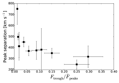
Figure 7: Observed separation between the red and blue Ly$\alpha$ peaks as a function of the residual flux in the central Ly$\alpha$ trough $F_{\mathrm{trough}}$ divided by the mean flux in the red and blue Ly$\alpha$ peaks $\bar{F}_{\mathrm{peaks}}$. An analogous plot was presented for model spectra in Gronke & Dijkstra (2016). No correlation was seen for clumpy models, while a trend was present for homogeneous shell models (see Sect. 5.4).

We devote the following sections to the exploration of possible reasons for the encountered discrepancies, discussion of the possible Ly$\alpha$ origin, and the compatibility of the observations with other existing models. We have searched for correlations between the fit parameter discrepancies and galaxy properties such as mass, size, metallicity, star-formation rate, amount of dust, UV absorption line $EW$s, emission, and absorption line $FWHM$. We found no clear trends.

5.1 Blue peaks in the literature

The unconstrained Ly$\alpha$ fits that we presented in Sect. 4.3.1 were previously studied by Yang et al. (2016), using the same GP sample and a similar set of homogeneous shell models (Dijkstra et al., 2006; Gronke et al., 2015). In this respect, the present paper reproduces their fitting results, while it further extends the analysis by applying observational constraints and by measuring the differences between the modelled and observed ISM parameters. In this paragraph, we compare the two sets of unconstrained fitting results produced by the two papers. Unlike the present paper, Yang et al. (2016) did not convolve the synthetic spectra to the observed spectral resolution, which could be the origin of several discrepancies. While our automatic procedure fitted all of the twelve Ly$\alpha$ profiles, Yang et al. (2016) were able to fit nine of them (their Figure 7). They reported that they manually adjusted the model parameters for the remaining three – GP 1133, GP 1219, and GP 1424 – to match the observed peaks and troughs. They published the model parameters for all twelve galaxies in their Table 4, which we now compare with our Table 3. The derived shell expansion velocities were similar in both studies (with differences between them of $\lesssim$ 50 km s^-1), and are equally inconsistent with the measured LIS outflows. Both studies needed similarly broad intrinsic Ly$\alpha$ profiles to achieve good fits (agreement between the two codes within $\sim$ 100 km s^-1). The third parameter causing problems in our fitting, the systemic redshift, was not discussed by Yang et al. (2016). They only presented the SDSS redshift in the paper and did not discuss any adjustments, therefore a comparison with our results cannot be done. No data were given for $EW_{0}$(Ly$\alpha$) in their paper either. Comparison between the derived H i column densities shows that in approximately one half of the sample the values agree between the two studies. In the other half, we typically find $N_{\mathrm{HI}}$ lower by $\sim\!\!1/2$ dex. We speculate that the reason lies in the absence of correction for spectral resolution in Yang et al. (2016); instead of broadening by the instrumental effect, their synthetic profiles needed to be additionally broadened by a higher $N_{\mathrm{HI}}$. For the dust optical depth $\tau_{\mathrm{d}},$ both papers show a large scatter in the best-fitting values for each target. The reason is a weak effect of the dust on Ly$\alpha$ in low-$N_{\mathrm{HI}}$ models ($N_{\mathrm{HI}}$ $\lesssim\!\!10^{19}$ cm^-2), which are characteristic of the GPs and which allow an efficient Ly$\alpha$ escape. Both dust-poor and dust-rich H i media can produce similar Ly$\alpha$ spectra if the $N_{\mathrm{HI}}$ is low, and are thus equally likely to be among the best-fitting models. Our median $\tau_{\mathrm{d}}$ values were lower by $\Delta\tau_{\mathrm{d}}\!\sim\!0.3\!-\!1$ than those of Yang et al. (2016) in one half of the sample, while they were either equivalent or higher by a similar amount in the other half. Given the large spread of $\tau_{\mathrm{d}}$ for each target, the values can be considered consistent between the two studies (with the exception of GP 0911), and also in agreement with the observations within the error bars. As for the Doppler parameter $b$ (which corresponds to the temperature in Yang et al., 2016), it is the least robust among the fitting parameters (Gronke et al., 2015), therefore a large scatter in the fitted values and large differences between the two codes would not be surprising. We see from the Yang et al. (2016) results that their model grid admitted temperatures as low as $10^{3}$ K, which was an order lower than in our code. We therefore automatically obtained fits with higher temperatures. In summary, we consider the results of the two unconstrained-fitting studies to be mostly consistent within the error bars. We generally considered larger error bars in order to account for the discreteness of the model grid and for the observational uncertainties, and also to provide sufficient parameter space for testing the match between the shell models, the ISM parameters, and the observational data.

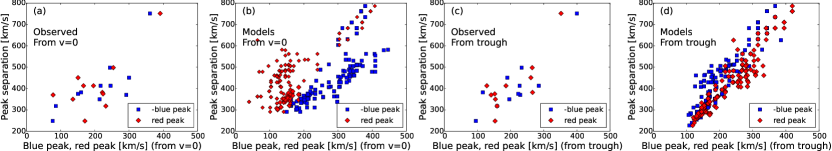
Figure 8: Symmetry of the red and blue Ly$\alpha$ peak positions in the observed and modelled spectra. a) The observed Ly$\alpha$ double-peak separation as a function of the blue and red Ly$\alpha$ peak positions: the distributions are similar for both peaks, the correlation is tighter for the blue peak, b) The same as (a) but for shell models; here the correlation is tighter for the blue peak, and the red and blue peaks are not symmetric. c) The same as (a) but measured with respect to the central Ly$\alpha$ trough; the correlations here are stronger than in (a). d) The same as (b) but measured with respect to the central Ly$\alpha$ trough; the asymmetry between the red and blue peaks disappears.

We also note here that problems with the double-peak Ly$\alpha$ profile fitting have been reported in the literature before. Chonis et al. (2013) had problems fitting double-peak profiles of $z\sim 2$ LAEs. However, we believe that those problems were mainly caused by the models that they used. Their radiative transfer code only computed the radiative transfer of monochromatic Ly$\alpha$ radiation, unlike ours that assumes a Gaussian line input plus a continuum. We are able to reproduce their LAE Ly$\alpha$ profiles with our model grid in the same way as the LBG spectra in Verhamme et al. (2008), Schaerer & Verhamme (2008), and as the GP spectra with unconstrained models in this paper. The problems that we encounter in our GP fitting are of a different nature: due to the availability of the detailed constraints we see the discrepancy between the fitted and observed ISM parameters. Such a detailed study has only been possible in the low redshift so far. Some of the constraints were available in the $z\sim 2$ LAE study of Hashimoto et al. (2015), where they also needed to invoke broad intrinsic Ly$\alpha$ to reproduce the blue peaks.

5.2 Stellar Ly$\alpha$

The double-peaked Ly$\alpha$ profiles observed in the GPs have their central troughs shifted in velocities compared to what was expected from the LIS absorption lines. In addition, some of the Ly$\alpha$ troughs are redshifted to positive velocities, unexpected in outflowing media. We have tested whether, despite the LIS line results, the unusual Ly$\alpha$ troughs could be explained by a combination of outflowing and infalling shell models The answer was negative. Infalling spherical H i shells with the Ly$\alpha$ source placed in the sphere centre would produce a redshifted trough, but the line profile symmetry would be opposite, with the blue peak dominating over the red (Verhamme et al., 2006; Dijkstra et al., 2006). A simultaneous production of a dominating red peak (as observed) and a redshifted trough (as observed) is challenging. We tested several scenarios that superposed infalling and outflowing shells, and none of them produced a redshifted Ly$\alpha$ trough for the given flux ratio of the red and blue peaks. We conclude here that the redshifted troughs probably point either to inconsistencies between the redshifts probed by Ly$\alpha$ and H$\beta$, or to ISM geometries not covered by our models, such as clumps, which we will discuss in Sect. 5.4. Related to this, Yang et al. (2016) discussed the possibility of infalling clumps, but with no direct proof or conclusion.

We have tested the possibility that the shift could be due to an underlying stellar Ly$\alpha$ absorption. Synthetic stellar population models using theoretical stellar atmospheres (Peña-Guerrero & Leitherer, 2013; Verhamme et al., 2008; Valls-Gabaud, 1993) showed that for a staburst $<$ 5 Myr, the stellar Ly$\alpha$ reaches absorption $EW$(Ly$\alpha$)${}_{\mathrm{stell}}\!\sim\!-4\pm 2$ Å, depending on the stellar model and on the star-formation regime. Such young starbursts are expected in our sample due to their large $EW$(H$\alpha$)  and were proven by stellar population fitting of similar targets in Izotov et al. (2016a, b). Therefore, the stellar Ly$\alpha$ absorption reduces the observed emission fluxes by $<\!\!10\%$ in most of our sample. Furthermore, the discrepancy of the trough position is the largest in the strongest Ly$\alpha$ emitters of our sample (Sect. 4.3.2), where the Ly$\alpha$ absorption will represent a particularly low fraction of the total flux. We have nevertheless tested the role of the stellar absorption on the final Ly$\alpha$ line profile, by matching Starburst99 models (Leitherer et al., 1999) of different ages and metallicities to our observational data. The synthetic spectra over-predict the Ly$\alpha$ absorption due to their use of observational O-star spectra, contaminated with interstellar features (Peña-Guerrero & Leitherer, 2013). With this in mind, we selected synthetic spectra that best matched the N v $\lambda 1240$ stellar P-Cygni feature. We subtracted them from the observed GP Ly$\alpha$ spectra. Even the over-predicted stellar Ly$\alpha$ absorption did not change the Ly$\alpha$ profile, namely, they did not shift the central trough position.

5.3 Galaxy compactness and Ly$\alpha$ halos

Numerical studies (Verhamme et al., 2012; Verhamme, 2015) have raised the possibility of Ly$\alpha$ double-peak formation in the Ly$\alpha$ “halos”, that is, in extended diffuse Ly$\alpha$ emission regions with no corresponding H$\alpha$ or stellar light. Radiative transfer in the cited hydrodynamic simulations showed that Ly$\alpha$ spectral profiles varied with the aperture size and position. Diffuse Ly$\alpha$ halos were observationally found in stacks of high-$z$ galaxies (Steidel et al., 2011; Momose et al., 2014), and confirmed in individual galaxies both at low and high redshift (Hayes et al., 2013, 2014, 2016; Wisotzki et al., 2016; Patrício et al., 2016).

The prevalence of double-peaks distinguishes the GPs from other galaxy samples. We can thus hypothesize that we see the effect of the Ly$\alpha$ halos here, similar to the simulations. GPs are compact galaxies, with the UV angular size generally smaller than the HST/COS aperture, unlike in the case of other local galaxies where the COS aperture contains the signal from one star-forming knot (such as in Wofford et al., 2013; Rivera-Thorsen et al., 2015). Thanks to the large COS Ly$\alpha$ escape fractions measured in GPs, we expect that Ly$\alpha$ does not scatter too far from the production sites and does not create large halos, and that most of their signal is contained in the COS spectra. However, whether or not the double peaks are due to the non-resolved nature of GPs and Ly$\alpha$ halos needs to be observationally tested in more detail. GP halos have so far been directly observed only for GP 0926 (Hayes et al., 2013, 2014), and has recently been suggested for other GPs based on the analysis of two-dimensional COS spectra (Yang et al., 2017b). The mechanism of the double-peak formation in the halos remains to be clarified, too. In the shell models, only a static or slowly expanding medium leads to the double-peaked Ly$\alpha$, therefore the role of kinematics must be assessed in the full simulation (see Verhamme, 2015). Furthermore, the Ly$\alpha$ halo emission can have an in-situ origin, either from cooling radiation or UV background fluorescence, rather than scattering (Cantalupo et al., 2012; Rosdahl & Blaizot, 2012; Dijkstra, 2014). If halos play a role in the Ly$\alpha$ profiles, then the encountered differences between LIS line and shell model velocities are unsurprising.

One could argue that high-$z$ galaxy spectra are typically spatially unresolved, and yet unlike in GPs their majority are single-peaked, while the incidence of multiple peaks is only $\sim$ 30% (Kulas et al., 2012; Trainor et al., 2015). However, the high-$z$ results are affected by the increasingly neutral IGM, which removes the blue part of the profile (Laursen et al., 2011), and also by a typically low spectral resolution that blends the two peaks into one (e.g. Kulas et al., 2012; Erb et al., 2014). Higher resolution data should alleviate at least one part of the problem. The connection between the blue peak and the Ly$\alpha$ halo is one of the tasks to be explored by both numerical simulations and observations. The galaxy size enters the problem in yet another aspect: the size of the Ly$\alpha$ photon source. The models that we used here assumed a point source. In contrast, the HST/COS acquisition images of GPs show a multi-knot star-formation structure in the near-UV. A similar structure will probably be reflected in the H ii regions, and therefore we need to ask how would this distribution affect the radiative transfer results. This effect has not been addressed in the homogeneous shell models and is a task for further modelling.

5.4 Clumpy shells and Ly$\alpha$ produced in outflows

Clumpy shell models (Laursen et al., 2013; Duval et al., 2014; Verhamme et al., 2015; Gronke & Dijkstra, 2016; Gronke et al., 2016, 2017) have demonstrated that the Ly$\alpha$ spectral profiles can be more complex than those from homogeneous shells. In particular, clumpy outflow geometries presented in Gronke & Dijkstra (2016) may provide an interesting alternative to the homogeneous shells, potentially solving several problems encountered in GP Ly$\alpha$ profile fitting (as was also invoked by Yang et al., 2016, 2017a).

First, in clumpy outflow models, the double-peaked Ly$\alpha$ profiles are not confined to low expansion velocities. This is a convenient property that would remove the conflict with the LIS line velocities and redshifts. Second, some of the clumpy models can achieve a redshifted central trough (Fig. 8 of Gronke & Dijkstra, 2016) – a property that is unachievable in homogeneous shells but is observed in some GPs. Third, the clumpy models may also remove the problem of the too broad intrinsic Ly$\alpha$, as shown by some of the results in Gronke & Dijkstra (2016). However, this may not be due to the clumpy nature of the model ISM, but rather due to the authors’ assumption that Ly$\alpha$ is formed inside the outflow, instead of a point source assumed in our models. More theoretical work needs to be done on the clumpy models to assess the blue and red peak locations and their asymmetries, as well as connections to the Ly$\alpha$ and LyC escape. A recent observation of a lensed $z=2.4$ galaxy reported a triple-peak Ly$\alpha$ spectrum, similar to clumpy models, and was interpreted as a possible LyC leakage signature (Rivera-Thorsen et al., 2017).

Nevertheless, we have designed a test to probe the usefulness of clumpy models for our GPs. Gronke & Dijkstra (2016) measured the residual flux in the modelled Ly$\alpha$ central trough $F_{\mathrm{trough}}$, and found that the ratio of $F_{\mathrm{trough}}$ and the mean of the peak maxima, $\bar{F}_{\mathrm{peak}}$, had a different distribution in the clumpy models than in the homogeneous shells (their Fig. 2). The ratio can span a wide range of values in the clumpy models, $F_{\mathrm{trough}}/\bar{F}_{\mathrm{peak}}\!\sim\!0-8,$ with the largest concentration around $F_{\mathrm{trough}}/\bar{F}_{\mathrm{peak}}\!\sim\!0.3.$ In contrast, $F_{\mathrm{trough}}/\bar{F}_{\mathrm{peaks}}\!<\!0.1$ for most of the homogeneous shell models. For comparison, our Fig. 7 shows that the observed GP $F_{\mathrm{trough}}/\bar{F}_{\mathrm{peaks}}\sim 0-0.3.$ These values could be explained by either model, since a small number of homogeneous models reach as far as $F_{\mathrm{trough}}/\bar{F}_{\mathrm{peaks}}\sim 0.6.$ In addition, the observational data may also be affected by instrumental resolution, which would make the observed $F_{\mathrm{trough}}$ artificially high. However, besides the interval span, the observed GP data inversely correlate with the Ly$\alpha$ double-peak separation (Fig. 7). No such correlation was found in the clumpy models; the models randomly filled all of the plane. Conversely, homogeneous shells showed a large scatter of peak separations ($v_{\mathrm{sep}}\!\sim\!0-2000$ km s^-1) at $F_{\mathrm{trough}}/\bar{F}_{\mathrm{peaks}}\sim 0$, but with increasing $F_{\mathrm{trough}}/\bar{F}_{\mathrm{peaks}}$ the maximum separation decreases to $v_{\mathrm{sep}}\!<$ 500 km s^-1 at $F_{\mathrm{trough}}/\bar{F}_{\mathrm{peaks}}\!\sim\!0.3$. The trend in homogeneous shells thus resembles the observed GP data (while bearing in mind that the sample size is limited). In homogeneous shells, both $F_{\mathrm{trough}}$ and the peak separation are governed by $N_{\mathrm{HI}}$, therefore a correlation between them is expected, unlike in the case of the clumpy models where Ly$\alpha$ escape is regulated by the properties and the distribution of the clumps.

In the view of these results, the role of the clumpy models is still unclear. A similarly hesitant conclusion was drawn by Gronke & Dijkstra (2016). The clumps are worth considering as they offer a multitude of possibilites (see also Gronke et al., 2016, 2017). Model fitting of observational profiles, using various flavours of the clumpy models, with and without constraining their parameters, remains to be done. Tests similar to our Fig. 7 could complement the spectral fitting.

5.5 Symmetries of the observed and modelled Ly$\alpha$ profiles

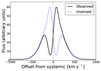
Figure 9: Model Ly$\alpha$ profile symmetries. The solid black line shows the shell model, the dashed blue line its inverse with respect to the systemic redshift. The shell model parameters: $N_{\mathrm{HI}}$ $=\!10^{18}$ cm^-2, $v_{\mathrm{exp}}$ $=50$ km s^-1, $\tau_{\mathrm{d}}\!=\!1$, $b\!=\!20$ km s^-1, $FWHM_{0}$(Ly$\alpha$) $=\!500$ km s^-1, $EW_{0}$(Ly$\alpha$) $=\!100$ km s^-1.

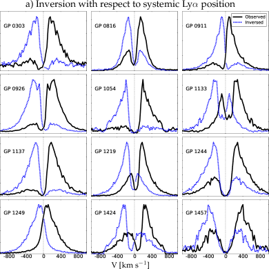
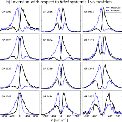
Figure 10: Observed Ly$\alpha$ profile symmetries: a) with respect to the systemic velocity derived from SDSS redshift, b) with respect to the systemic velocity derived from best-fitting model. The solid black line shows the observed data, the blue line their inversion. The red and blue wings are more symmetric in case (b) than in case (a).

We here explore symmetries of the shell model Ly$\alpha$ profiles and compare them with those observed in the GPs. Symmetries in peak positions, wings, and troughs could provide additional insight into the incompatibilities between the GP data and shell models or their parameters.

It was noted by Henry et al. (2015) that it is mainly the blue-peak position that correlates with the GP double-peak separation, and thus with the Ly$\alpha$ and LyC escape (Verhamme et al., 2015, 2017). Yang et al. (2017a) then showed that both peaks correlate with $f_{\mathrm{esc}}$(Ly$\alpha$) in a larger GP sample. We here test if the same is true for the models. We work with twelve GPs, therefore we have to bear in mind the effects of the limited sample size. We presented the GP asymmetric blue and red Ly$\alpha$ peak positions in Fig. 1. We here study the Ly$\alpha$ double-peak separation versus the blue and red peak positions measured from the systemic redshift both in the observed and modelled spectra (Fig. 8a,b). The double-peak separation is a proxy for the Ly$\alpha$ and LyC escape, and we explore how the blue and red peaks correlate with it and what symmetries exist in the observations and the models. We include the shell models that were among the twenty best fits for each target (see Section 4.3). We find stronger correlations for the blue peak both in the COS data and in the models. However, a clear shift between the red and blue peak positions exists in the models, not seen in the observations. Models with strong blue peaks (blue-to-red flux ratio $>0.3,$ Table 2) have the most symmetric peak positions (i.e. red and blue squares plotted close to each other in Fig. 8b). Conversely, the weak blue peak models are responsible for the scatter in that plot. On the other hand, if we measure the peak positions from the central trough, instead of the systemic velocity, then we obtain plots of Fig. 8c,d. Both the observed and modelled spectra show more symmetry with respect to the trough than to the systemic velocity. The correlation with the peak separation is strong for both the blue and red peaks and for both the observed and modelled spectra in this case. This result is another illustration of why our models failed to reproduce the observed spectra with applied constraints, while they were usable in the modelling with free redshift; they attained the required symmetry with the modified redshift. Using the modified redshift, the blue and red peak positions would resemble the models in Fig. 8b.

We have further tested the symmetry of the Ly$\alpha$ line wings by exploring the Ly$\alpha$ profiles together with their plots flipped with respect to the systemic velocity (Figs. 9 and 10). The modelled double-peaks have symmetric wings with respect to the systemic redshift (Fig. 9) but with the condition of a broad $FWHM_{0}$(Ly$\alpha$), equivalent to the one that fits the observed GP profiles. The wing symmetry is created by small effects of radiative transfer far from the line centre, and by a symmetric intrinsic profile. On the other hand, models with a narrow $FWHM_{0}$(Ly$\alpha$) (as in Fig. 2) have red wings stronger than the blue ones, due to radiative transfer effects. For the observed GP spectra, the red wing is also mostly stronger than the blue one (Fig. 10a), despite the fact that the wings are as broad as in the model of Fig. 9. On the contrary, if we consider $z$ derived from the Ly$\alpha$ fits rather than SDSS, the observed wings become symmetric (Fig. 10b).

We conclude that the free fitting process modifies $z$ to obtain spectra that are more symmetric in the red and blue peak position with respect to the systemic redshift. The new symmetry makes the data compatible with the shell models. As a consequence, the line wings become symmetric. The wing symmetry of the model spectra is in turn achievable by assuming a large intrinsic $FWHM_{0}$(Ly$\alpha$). A comparison with clumpy models and other geometries would be useful to assess how unique is the symmetry resemblance between the data and the shifted models, resulting in the alignment of the trough position and wing shape, and in the possibility of finding models that fit the double peaks. This exercise still does not clarify the reasons for the discrepancy in $z.$ It does not answer the question of how appropriate the shell models are, or if the resemblance between the unconstrained fitting models and the data is a coincidence. We showed in Section 4.3.2 that the discrepancies in individual fitting parameters were tied to the spectral shape, namely to the blue peak $EW$. We also showed that the blue peaks were related to Ly$\alpha$ and LyC escape. In this light, the resemblance between symmetries of modelled and observed (shifted) spectra appears surprising and requires more theoretical work.

5.6 Ly$\alpha$ sources

Our models considered recombination as the only source of Ly$\alpha$. Some of the fitting parameter discrepancies, namely in $z$ and $FWHM_{0}$(Ly$\alpha$), were evaluated by comparing the Ly$\alpha$ and H$\beta$ lines under the assumption that the same recombination process was the origin of both lines. However, other Ly$\alpha$ production mechanisms are possible and could be responsible for part of the fitting problems.

Collisional excitation is one such process that could cause kinematic differences between Ly$\alpha$ and H$\beta$. Collisional excitation affects more the first excited level than the higher energy levels, leading to the Ly$\alpha$/H$\alpha$ emissivity ratio $\sim\!\!100$ (Dijkstra, 2014), that is, an order of magnitude higher than in the case of recombination ($\sim\!\!8$). In violent conditions inside GPs, characterized by large star-formation rates and high excitation, strong collisional processes can be expected (Otí-Floranes et al., 2012). Typical GP electron temperatures are relatively high, $\sim\!\!15\,000$ K, favourable to the collisional excitation scenario (Jaskot & Oey, 2013). Collisional contribution could explain the intrinsic Ly$\alpha$ profile broadening and the redshift discrepancy between the modelled intrinsic Ly$\alpha$ and the observed H$\beta$. We have also previously mentioned the possibility of Ly$\alpha$ production in outflowing medium (Sect. 5.4), which could be due to a number of different processes; their impact on the resulting spectrum needs to be further explored.

Other possible sources of Ly$\alpha$ emission include fluorescence (Cantalupo et al., 2012, 2014) and gravitational cooling (Dijkstra et al., 2006; Dijkstra, 2014). Both processes, acting in the outer layers of the ISM, would be able to produce a large $FWHM_{0}$(Ly$\alpha$) (Hashimoto et al., 2015). In addition, Fermi-like acceleration of Ly$\alpha$ photons across shock fronts was suggested as an alternative origin of the Ly$\alpha$ blue peaks (Chung et al., 2016; Neufeld & McKee, 1988). Tests for these predictions are still missing. Martin et al. (2015) searched for the signatures of Fermi acceleration in ULIRGs and concluded that no compelling evidence was found, but they admitted that the process can play a role in some objects.

Finally, we note that a detailed exploration of the recombination sources alone would also be useful. The SDSS H$\beta$ spectra that we used did not have sufficient resolving power ($R\!\sim\!2000$) to show the complete emission line structure. Amorín et al. (2012) observed several green peas with a high-resolution echelle spectrograph ($R\!>\!\!10\,000$), and found complex H$\alpha$ profiles with several distinct kinematic components. If the components come from different regions of the galaxy, conditions for the Ly$\alpha$ transfer in each of them can be different and could thus affect differently the resulting Ly$\alpha$ profile. The sample of Amorín et al. (2012) unfortunately does not overlap with our Ly$\alpha$ sample and thus could not be tested.

6 Summary and conclusions

We have studied in detail the Ly$\alpha$ spectra of twelve green pea galaxies, which are an unusual population of strongly star-forming compact galaxies at $z\sim 0.2,$ and which resemble high-redshift Ly$\alpha$ emitters in their mass, metallicity, star-formation rate, and possibly ionizing continuum leakage. Eleven out of the twelve studied GPs have double-peaked emission-line Ly$\alpha$ spectral profiles. The spectra show no signs of broad underlying Ly$\alpha$ absorption (which is often observed in low-$z$ star-forming galaxies), with two weak exceptions. Furthermore, they have non-zero residual flux in the central trough that separates the blue and red peaks. Together with a small peak separation, these properties indicate low H i column densities, based on the criteria of Verhamme et al. (2015). The central Ly$\alpha$ trough is redshifted from the systemic velocity in several GPs, which is unusual in the context of the known observations and models.

We applied the MCLya Monte Carlo Ly$\alpha$ radiative transfer code (Verhamme et al., 2006), which uses the geometry of expanding homogeneous shells, to fit the GP Ly$\alpha$ spectra and derive their ISM parameters. In the first step, we applied detailed constraints on the fitting parameters, inferred from ancillary UV and optical spectra. The models did not correctly reproduce the observed GP Ly$\alpha$ spectra in this case (Fig. 2). We thus proceeded to unconstrained fitting (similar to Yang et al., 2016, 2017a), which correctly reproduced the spectral profiles (Fig. 4), but the best-fitting model parameters were in disagreement with the ancillary data (Fig. 5). In particular: 1) The redshifts derived from the Ly$\alpha$ fitting were in all cases larger than those from the SDSS optical emission lines ($\Delta z\!=\!10\!-\!250$ km s^-1); 2) The best-fit outflow velocities were typically $\lesssim\!150$ km s^-1, whereas the UV LIS line velocities were distributed in the interval $0-300$ km s^-1; 3) The modelled $FWHM_{0}$(Ly$\alpha$) of the intrinsic Ly$\alpha$ line was a factor of two to four larger than the measured $FWHM$(H$\beta$) in each target. We found a link between the fit parameter discrepancies and the double-peak character of the Ly$\alpha$ profiles, namely the $EW$(Ly$\alpha$)_Blue/$EW$(Ly$\alpha$)_Red ratio of the blue and red peak equivalent widths (Fig. 6).

We propose two interpretations for the data-model disagreement. First, the ancillary data may be inappropriate to constrain the models; the LIS lines may not probe the environment where the Ly$\alpha$ transfer takes place and the intrinsic Ly$\alpha$ may not be produced by the same mechanism as H$\beta$. We showed that by modifying $z,$ the observed Ly$\alpha$ trough positions would become compatible with the models (Fig. 6b) and the observed Ly$\alpha$ profile symmetries would correspond to those of the homogeneous shell models (Figs. 8-10). Second, the blue Ly$\alpha$ peaks of GPs may not originate in a static ISM, as is the case in the homogeneous shell models, or at least not in the gas probed by the UV LIS lines. The blue peak formation mechanisms, either at a source or by the radiative transfer, need to be further investigated. The $EW$(Ly$\alpha$)_Blue/$EW$(Ly$\alpha$)_Red ratio correlates with the Ly$\alpha$ escape fraction, and with the Ly$\alpha$ peak separation, which suggests that the GP blue peaks are associated with low $N_{\mathrm{HI}}$, and with the Ly$\alpha$ and LyC escape, rather than kinematics. A connection between the blue peak position and $N_{\mathrm{HI}}$ was previously proposed in the literature (Henry et al., 2015; Yang et al., 2016, 2017a), while we here extend this effect to the blue peak flux.

We considered alternative models to reproduce the GP Ly$\alpha$ profiles. No combination of outflowing and inflowing homogeneous shells was found to be compatible with the observed GP spectra. Clumpy models such as those of Gronke & Dijkstra (2016) are a promising option, as they produce double peaks of various shapes by other mechanisms than kinematics. However, more theoretical work is needed to check their compatibility with observations. We could not confirm the compatibility based on the measured residual flux in the central trough of Ly$\alpha$ spectra. We found that it correlates with the red-blue Ly$\alpha$ peak separation in GPs, which is a trend expected in the homogeneous case and not in the clumpy models (Gronke & Dijkstra, 2016). Nevertheless, the small observational sample may only cover a portion of the parameter space and a larger sample will be needed to extend this study. Also, various versions of the clumpy models may provide different results.

For future work, high-resolution H$\alpha$ or H$\beta$ spectra would be useful to provide more details about the H ii regions kinematics, that is, about the Ly$\alpha$ source. If multiple kinematic components are present, their impact on the resulting Ly$\alpha$ profile needs to be explored in the models. Possible contributions of non-recombination processes to the Ly$\alpha$ spectra need to be tested. Finally, model fitting with the use of clumpy geometries should clarify whether the clumps are a solution to the problem of mismatching ISM parameters.